prepared in cooperation with the mojave water agency u.s. … · 2010-10-23 · water resources...

UNITED STATES DEPARTMENT OF THE INTERIOR

GEOLOGICAL SURVEY Water Resources Division

HYDROLOGIC ANALYSIS OF

MOJAVE RIVER BASIN, CALIFORNIA

USING ELECTRIC ANALOG MODEL

By

William F. Hardt

Prepared in cooperation with theMojave Water Agency

U.S. Marine Corps Supply Center, Barstow George Air Force Base

OPEN-FILE REPORT00o

ioo oCM

Menlo Park, California August 18, 1971

CONTENTS

PageAbstract 1Introduction 3Regional setting 5Well-numbering systern 9Geohydrology of the modeled area 10

Geology of the aquifer 11The Mojave River 12Boundary conditions 20Aquifer transmissivity and storage coefficient 22

Analysis of the hydrologic system by the electric analog model 27Basis of the electric analog model 29Verification of the model 39

Steady-state conditions 39Non-steady-state conditions 45

Model predictions and results 58No aquifer recharge, storage depletion, 1930-63 60Basin-wide water-level changes with extremes in Mojave River flow,1930-2000 62

Effects of pumping a well field 70Effects of artificial recharge on river system 73

Conclusions 78Selected references 81

ILLUSTRATIONS

Page Figure 1. Index map 3

2. Map showing geology of study area 63. Chart of precipitation and potential evapotranspiration 84. Map showing hydrology of study area 135. Graph of cumulative departure of precipitation, 1910-68 146. Graph of flow characteristics in Mojave River between

The Forks and Victorville, 1931-68 187. Graph of double-mass curves of Mojave River flow, 1931-68 198. Map showing aquifer transmissivity and storage

coefficient In pocket9. Chart showing use of analog model 27

10. Sketch of basis of electric analog model 3311. Diagrammatic representation of flow system and analog model 35

III

IV CONTENTS

Page Figure 12. Grid for model 37

13. Photographs of the analog model 38 14-16. Maps showing:

14. Ground-water level, 1930 40

15. Model ground-water level, 1930, including Mojave Riversimulation 44

16. Ground-water level, spring 1964 46

17. Graph of consumptive-use pumpage in model, 1930-63 4918. Chart of estimated consumptive use of total pumpage 50

19-21o Maps showings19. Location of model pumpage nodes, 1930-63 5120. Water-level decline, 1930-63 5221. Model water-level decline, 1930-63 56

22. Graph showing selected well and model hydrographs 5723. Map showing model water-level decline, 1930-63, with no

recharge and ground water pumped from storage only 61 24 0 Map showing selected model hydrographs, 1930-2000 In pocket

25-27o Maps showing model water-level decline:25. 1930-2000 6626. 19 70-80 6827. 1970-2000 69

28. Map showing model effects of high rate, short durationpumping In pocket

29. Map showing model study of imported water recharge onriver system In pocket

TABLES

Page Table 1. Streamflow in Mojave River at selected stations, 1931-68 16

2. Peak discharges in Mojave River, 1932-69 173. Summary of laboratory core analyses 264. Water budget, 1930 and 1963 425. Detailed water budget for Mojave River, 1930 and 1963 436. Ground-water pumpage, by areas, 1930-63 487. Estimated change in ground-water storage, 1930-69 538. Model predictions, 1930-2000 639. Annual imported water entitlements, California Water Plan,

1972-90 73

I

HYDROLOGIC ANALYSIS OF MOJAVE RIVER BASIN, CALIFORNIA, USING

ELECTRIC ANALOG MODEL

By William F. Hardt

ABSTRACT

The water needs of the Mojave River basin will increase because of population and industrial growth. The Mojave Water Agency is responsible for providing sufficient water of good quality for the full economic development of the area. The U.S. Geological Survey suggested an electric analog model of the basin as a predictive tool to aid management.

About 1,375 square miles of the alluvial basin was simulated by a passive resistor-capacitor network. The Mojave River, the main source of recharge, was simulated by subdividing the river into 13 reaches, depending on intermittent or perennial flow and on phreatophytes. The water loss to the aquifer was based on records at five gaging stations. The aquifer system depends on river recharge to maintain the water table as most of the ground-water pumping and development is adjacent to the river.

The accuracy and reliability of the model was assessed by comparing the water-level changes computed by the model for the period 1930-63 with the changes determined from field data for the same period.

The model was used to predict the effects on the physical system by determining basin-wide water-level changes from 1930-2000 under different pumping rates and extremes in flow of the Mojave River. Future pumping was based on the 1960-63 rate, on an increase of 20 percent from this rate, and on population projections to 2000 in the Barstow area. For future predictions, the Mojave River was modeled as average flow based on 1931-65 records, and also as high flow, 1937-46, and low flow, 1947-65.

Other model runs included water-level change 1930-63 assuming aquifer depletion only and no recharge, effects of a well field pumping 10,000 acre- feet in 4 months north of Victorville and southeast of Yermo, and effects of importing 10,000, 35,000, and 50,800 acre-feet of water per year from the California Water Project into the Mojave River for conveyance downstream.

2 ELECTRIC ANALOG MODEL, MOJAVE RIVER BASIN, CALIF.

Analysis of the hydrologic system in the Mojave River.basin, using the electric analog model, indicates that the long-term pumping is exceeding natural recharge, the water table is declining, and an overdraft or aquifer depletion is occurring. Ground-water pumpage was about 40,000 acre-feet in 1930 and more than 200,000 acre-feet in 1963. The depletion is only 1-2 percent of the water in storage. Unfortunately, the depletion is not uniform throughout the basin but is localized because of pumping in the developed parts of the basin. Areas of maximum water-level declines are near Harper Lake, Hinkley, and Daggett, and east of Hesperia.

The model showed that the boundary conditions in the aquifer, such as faults, configuration of the basin, large variations in aquifer transmissivity, recharge areas, and pumping patterns, have a pronounced effect on water-level changes. In general, the water-level declines to the year 2000 are approximately straight-line projections of the documented decline from 1930 to 1963.

The upper basin gets first opportunity for replenishment because of its proximity to the main sources of recharge, the headwaters of the Mojave River, and runoff from the San Bernardino-San Gabriel Mountains. These areas account for about 97 percent of the basin recharge. A geohydrologic anomaly along the Mojave River near The Forks in the upper basin indicates that a confining layer of low permeability hinders river recharge to the deeper aquifer, as evidenced by maximum declines east of Hesperia. Downstream, perennial flow in the river for 15 miles in the Victorville area has stabilized water levels.

The model indicates that if floodflows are not available to replenish the aquifer, the Hinkley-Barstow-Daggett area may experience water deficiencies earlier than other parts of the basin. The reasons are greatly increased pumping predicted in the Barstow area, and low storage capacity of the aquifer with its narrow, highly permeable channel between the mountains. The aquifer boundary and its small cross-sectional area cause large water- level fluctuations from pumping patterns or flood sequences. East of Daggett the aquifer is wide and deep, and long-term water levels will not fluctuate greatly under proposed future pumping patterns. Much of the water pumped is from storage in the aquifer, so continued minimal water-level declines are anticipated.

Wet and dry climatic periods result in extremes of flow in the river and in different rates of water-level change. Flow in the Mojave River accounts for about 80 percent of the recharge to the basin, and 85 percent of the average flow (1931-68) entering the basin at The Forks remains upstream from Afton. Generally less water becomes available downstream, and the influence of the river as a conduit system diminishes. Low flows do not normally reach Barstow because the river channel is highly permeable and susceptible to recharge. Most of the recharge to the aquifer downstream from Barstow results from floods. From 1931 to 1968 only 27 percent of the water that entered the basin at The Forks reached Barstow, and that mostly during the floods of 1932, 1937-38, 1941, 1943-46, 1952, 1958, and 1965-66.

The analog-model analysis should be regarded as the beginning of a new phase of geohydrologic study in the Mojave River basin. The knowledge gained from this initial model study will be helpful in formulating programs of

INTRODUCTION

better data collection, as well as testing concepts of the flow system under varied conditions. Hydrologic modeling should be a part of the total management program, as the model can be continually updated and improved.

INTRODUCTION

The Mojave River basin is in the Mbjave Desert region of southern California about 80 miles northeast of Los Angeles (fig. 1). Like similar desert regions in the southwestern part of the United States, the Mbjave River basin has accelerated in population and industrial growth during the 1960 f s. The proximity of the Mojave Desert region to the highly urbanized Los Angeles complex will be a stimulus to economic growth in the desert as land in the coastal areas becomes unattainable and costs continue to rise. Economic studies of the basin suggest an increasing rate of growth in the future, provided adequate supplies of water of good quality are available. The water supply for the present economic development comes from surface water in the Mojave River and from the large quantity of ground water stored in the alluvial aquifers.

124' 123- 122' 121" 120"

> o

REA OF REPORT

120° 119° 115-

30 o so

FIGURE 1. Index map


Recent hydrologic studies of the basin indicate that ground-water discharge, mainly from pumping by wells, exceeds the natural recharge, and consequently the water table is declining in many parts of the basin. Although a large quantity of water is stored in the basin, a potential deficiency in water supply is possible and is of concern to farmers, industry, water purveyors, and the public. To remedy this potential deficiency and to provide for better management of the water resources, the Mojave Water Agency was authorized by the State Legislature and created by a vote of the people within the Mojave Desert area in 1960. To provide sufficient water for future economic development to the year 1990 or later, the agency has contracted with the State to purchase water from the California Aqueduct starting in 1972 if the water is needed to augment the local natural supply.

The general purpose of this study was to aid the Mojave Water Agency in fulfilling its obligation to the people by efficiently managing all the water resources within its boundaries. The agency's program includes utilization of the ground-water reservoirs, the Mojave River, imported California Aqueduct water, and reclamation of sewage and waste water. The agency's main purpose is to see that sufficient water of acceptable quality is distributed to all present and potential customers.

As an aid for solving technical water problems in the Mojave River basin and predicting alternatives, an analog model was constructed. The model's primary purpose is to simulate the flow pattern of ground water and the change in water levels with time due to pumping and river recharge in the physical system. Any theoretical or alternative set of water-use conditions can be programed into the model, and the effects on the water table measured, although precise answers are not always possible due to the inexactness of the field data that are simulated in the model. These predictions can be done quickly and at low cost compared with detailed field studies with trial-and- error methods where costs in time and money can be great. The analog model may be refined as more precise information is available. The present analysis should be regarded as the beginning of a new phase of hydrologic study of the Mojave River basin, and not as the study that ends all studies.

The scope of the study included (1) gathering and analyzing available geohydrologic data, (2) obtaining needed additional data by field studies or test drilling, (3) converting these data for use in an electric analog model, (4) constructing and operating the model, (5) verifying and refining the model by updating the field studies, (6) predicting hydrologic cause-and- effect relations, and (7) a continuing program of answering specific hydrologic questions that may come up.

The scope also included the study of additional hydrologic parameters obtained from the field and the model, such as (1) recharge water from the Mojave River and the California Aqueduct, (2) head measurements and rates of inflow and outflow at the boundaries, (3) evaluation of the aquifer transmissivity and storage coefficient, (4) effects of phreatophytes on the hydrologic system, (5) discharge rates from the dry lakes, and (6) areas of productive wells.

REGIONAL SETTING 5

Technical problems answered by the model include (1) the importance of the Mojave River as a source of ground-water recharge to the basin, (2) predictions of basin-wide water-level changes based on different pumping regimens, (3) prediction of water-level change in the aquifer system caused by extended floods (high flow) and droughts (low flow) in the Mojave River, (4) effects on the aquifer system of high-rate, short-term pumping at selected locations, and (5) future water-level changes caused by recharge of imported water from the California Aqueduct into the Mojave River, and the distance the surface water moves downstream.

This study and report were made in cooperation with the Mojave Water Agency; U.S. Marine Corps Supply Center, Bars tow; and George Air Force Base. The work was done during 1966-70 by the U.S. Geological Survey, Water Resources Division, under the general direction of R. Stanley Lord, district chief in charge of water-resources investigations in California, and the immediate direction of L. C. Dutcher, J 0 L, Cook, and R 0 E. Miller, successive chiefs of the Garden Grove subdistrict. The analog model was constructed and analyzed by Geological Survey personnel at Phoenix, Ariz. s under the supervision of E. P. Patten, and valuable x^ork was contributed by Stanley Longwill, Michael Field, and Joseph Reid.

REGIONAL SETTING

The Mojave River (fig. 2) is the main stream traversing the study area and is the main source of recharge to the aquifers. The river originates in the San Bernardino Mountains and joins Deep Creek at the base of the mountains at an altitude of about 3,000 feet above mean sea level. The junction of the two rivers is called The Forks. The river flows northward through Victorville, then eastward through Bars tow, and leaves the basin at Afton at an altitude of about 1,400 feet above mean sea level and about 100 miles downstream from The Forks. The land-surface gradient of the Mojave River is 15-20 feet per mile a On the sides of the valley the slopes are steeper, and tributary washes with gradients of 50-100 feet per mile are common. Recharge to the basin from most of the tributaries is not significant.

The climate of the Mojave River basin is typical of arid regions of southern California. It is characterized by low precipitation, low humidity, high summer temperatures, and strong winds at certain times of the year. These climatic factors combine to cause high evaporation rates from open-water surfaces and soil-moisture deficiences in the unsaturated zone above the water table.

ELECTRIC ANALOG MODEL, MOJAVE RIVER BASIN, CALIF,

AHVN -3Hd QNVAHVUH31

4J 0)

CM

oM

REGIONAL SETTING 7

Generally, rainfall in the Mojave River basin occurs in two characteristic patterns. About 70 percent of the average annual rainfall at Victorville and Barstow occurs from November through March. The winter storms generally move from the Pacific Ocean eastward, are as much as 4 to 5 days in duration, and come when crops are mostly dormant. Therefore, the soil-moisture content in the unsaturated zone may be higher in the winter than in the summer. The summer rains are short, intense, and more local, and come from thunderstorms that move up from Arizona. Summer rainfall is of little value to agriculture because there is so little rain and evaporation losses are high.

Data from the National Weather Service (U.S. Weather Bureau) indicate that the mean annual precipitation at Victorville and Bars tow for 1939-68 was 4.97 and 4.16 inches, respectively. Recharge to the aquifers from direct precipitation on the desert floor probably is negligible. The mean annual temperature at Victorville for 1940-65 was 59.6°F (15.4°C), and the mean monthly temperature ranged from 42.6°F (5.9°C) in January to 78.7°F (26.0°C) in July. At Bars tow for 1924-65 the mean annual temperature was 64.1°F (17.8°C), and the mean monthly temperature ranged from 45.9°F (7.7°C) in January to 84.5°F (29.2°C) in July. In July and August midday temperatures in the basin are frequently more than 100°F (37.8°C).

In arid and semiarid regions, the quantity of water that actually evaporates and transpires from the soil is less than the potential because water is not always available. Thornthwaite (1948) devised a method for computing potential evapotranspiration from the soil based on mean monthly temperatures and the latitude of the area. These data were compared to the mean monthly precipitation of the Mojave River basin (fig. 3). The climatological data for Victorville and Bars tow were averaged to represent the desert region of the basin. Precipitation exceeds potential evapotranspiration during only 3 months of the year (January, February, and December), and then only by a slight amount. The computed potential evapotranspiration from the soil was about 35-1/2 inches per year or 7-1/2 times greater than the annual precipitation. Figure 3 shows the high ratio of potential evapotranspiration from soil to precipitation available for recharge to the aquifers from the desert floor.

Evaporation from a National Weather Service class A evaporation pan for 1931-33 averaged about 83 inches per year (Blaney, 1933, p. 24) at a station on the east side of the Mojave River at the upper narrows near Victorville. The annual evaporation from the Mojave River surface is about 5 feet, or 1-1/2 times greater than the computed potential evapotranspiration from the soil. Water loss from the river surface is greater than from the soil because of high air temperature, low atmospheric humidity, and wind action on the water. Soil cover reduces the effectiveness of these parameters and lessens water loss.

ELECTRIC ANALOG MODEL, MOJAVE RIVER BASIN, CALIF.

Precipitation, National Weather Service (U.S. Weather Bureau), records averaged for stations at Victorville (1938-65) and Barstow (1889-97; 1903-20; 1939-65). Potential evapotranspi ration from Thornthwaite method (1948)

EXPLANATION

Precipitation, in excess of potential evapotranspi ration

Potential evapotranspiration in excess of p recipi tation

Mean monthly precipitation for March through November. Mean monthly evapotranspi ration for January, February, and December

FIGURE 3. Precipitation and potential evapotranspiration.

ELECTRIC ANALOG MODEL, MOJAVE RIVER BASIN, CALIF,

WELL-NUMBERING SYSTEM

The we11-numbering system used in the Mojave River basin has been used by the Geological Survey in California since 1940, and is in accordance with the Bureau of Land Management's system of land subdivision. The system has been adopted by the California Department of Water Resources, California Water Pollution Control Board, and many local water districts. As shown by the diagram, that part of the number preceding the slash, as in 9N/2E-13Q1, indicates the township (T. 9 N.); the number following the slash indicates the range (R. 2 E.); the number following the hyphen indicates the section (sec. 13); the letter following the section number indicates the 40-acre subdivision according to the lettered diagram. The final digit is a serial number for wells in each 40-acre subdivision and indicates the first well to be listed in the SW%SE% sec. 13, T. 9 N., R. 2 E. The area covered by this report lies east and west of the San Bernardino meridian and north of the San Bernardino base line (fig. 2).

R.2 W. R.I W. R.I E. R.2E. R.3 E.

T.I2N.

T.IIN.

T.ION.

T.9N.

T.8N.

T.7N.

z

o

u£

Oz

zUJtoz

>x

X

N

^>,

N

\\

67

18

19

3031

58

17

20

2932

49

16

21

2833

310

15

22

27

34

2II

14

23

26

35

112

^3

\425

36 D

E

M

N

C

F-1 L

P

B

G

K

^

A

H

J

9$?E -I3QI

10 ELECTRIC ANALOG MODEL, MOJAVE RIVER BASIN, CALIF,

GEOHYDROLOGY OF THE MODELED AREA

The geohydrology of the Mojave River basin has been described in previous reports (California Department of Water Resources, 1967; Thompson, 1929; Miller, 1969; and Kunkel, 1962). This section describes and analyzes only that geohydrologic information pertinent to the construction, verification, and operation of an electric analog model. During the geohydrologic analysis, and particularly during the many model runs, several anomalies became apparent in the available data. Thus the model was helpful in developing ideas and enhancing knowledge of the geology and hydrology. The use of the geohydrologic data will be more fully described in the section on analysis of the hydrologic system by the electric analog model.

About 1,375 square miles of the Mojave River basin is simulated by the electric analog model. Previous hydrologic studies have, for convenience, arbitrarily divided the Mojave River basin into the upper, middle, and lower Mojave, and Harper Lake (fig. 2). All the modeled area is an alluviated plain, sloping gently northeastward, with ground water stored in the basin sediments. Hydrologically, the study area is one flow system and extends from The Forks at the base of the San Bernardino Mountains to Afton and includes the dry Harper, Coyote, and Troy Lakes. Part of the basin is undeveloped, but historically, most of the irrigable lands and centers of population, such as Victorville and Barstow, are adjacent to the Mojave River. Surrounding the ground-water basin are the consolidated rocks of the mountains, mainly non-water-bearing crystalline and metamorphic rocks.

The physical system of the basin includes the hydrology of the Mojave River; variations in geologic framework, both laterally and vertically; the boundary or perimeter of the study area; and the aquifer properties of hydraulic conductivity (permeability), transmissivity, and storage. These characteristics of the basin are essential for the solution of cause-and- effect relations in the model.

Prior to man's extensive development the ground-water flow system for the model study was considered to be in equilibrium, with recharge equal to discharge and no permanent change in ground-water storage. This is not exactly correct, as the hydrologic system is a dynamic condition resulting from flow in the Mojave River during extremes of wet and dry periods. However, the long-term hydrologic changes were considered as minor. After development by pumping of wells the flow system was measurably unbalanced, and recharge and discharge conditions changed from the natural state. The geohydrology under natural and steady-state conditions will be described under the section, verification of the model.

GEOHYDROLOGY OF THE MODELED AREA 11

Geology of the Aquifer

The geologic units are grouped into two broad categories (1) consolidated non-water-bearing rocks, and (2) unconsolidated water-bearing deposits. The consolidated rocks comprise the mountain ranges that surround the alluvial plains of the basin (figo 2), They include metamorphic and igneous rocks, of pre-Tertiary age, which, except for minor quantities of water in cracks and weathered zones, are considered non-water-bearing. These rocks are primarily outside the modeled area and are not discussed further. The unconsolidated deposits underlie the basin within the mountain boundaries. These deposits are highly permeable, transmit ground water, constitute the subsurface storage reservoir for ground water, and were modeled for this study.

The unconsolidated water-bearing deposits range in size from coarse gravel to clay and are generally less permeable with depth. The deposits in the valley result primarily from erosion in the adjacent mountains. The mountain streams carry debris onto the valley floor during floodflows, forming alluvial fans at the base of the mountains. As the distance from the mountains becomes greater, the stream gradients and water velocity become less, and the sediment-carrying capacity of the stream becomes less, resulting in deposition of finer-grained material, such as silt and clay, in the lowest part of the basin. This general deposition pattern is interrupted by the Mojave River traversing the valley and cutting a channel through both coarse and fine-grained material, and then refilling with coarse-grained, permeable river deposits.

Geologically, the age of the unconsolidated deposits ranges from Pleistocene to Holocene. These sediments are divided into Mojave River deposits, playa deposits, dune sand, younger alluvium, younger fan deposits, old lake and lakeshore deposits, older alluvium, older fan deposits, landslide breccia, Shoemaker Gravel, and the Harold Formation.

The Mojave River deposits and the older alluvium are important to the analog model because of their water-bearing characteristics, large areal extent, and relation to ground-water development. The Mojave River deposits are the most important aquifer and probably the most permeable of any of the geologic units. The deposits range from 1/4 to 1-1/2 miles wide, accept river recharge, and yield most of the ground water pumped in the basin. The river deposits include boulders, gravel,, sand, and silt with some clay and are as much as 200 feet thick. Well yields from these deposits generally range from 100 to 2,000 gpm (gallons per minute) and average about 500 gpm. Wells drilled in 1970 about 6 miles west of Barstow have been tested at 4,000 gpm. With proper well construction and development, unusually high yields are possible in these deposits.


The older alluvium underlies most of the study area and ranges from a few inches to about 1,000 feet thick. This unit contains most of the ground water in storage. The deposits range from unconsolidated to moderately consolidated and consist of interbedded gravel, sand, silt, and clay. The deposits are weathered, and some cementation has developed, mostly in the form of caliche. The yield of wells from these deposits varies considerably depending on the permeability of the alluvium. For example, wells near Hesperia and Daggett yield more than 2,000 gpm, whereas, wells north of Adelanto yield about 25 gpm or less.

The other geologic units are of lesser hydrologic importance in the model analysis because they are generally above the water table or localized in the basin.

The Mojave River

About 92 percent of the long-term recharge to the Mojave River basin originates in the San Bernardino Mountains. Tributary runoff from the San Gabriel Mountains contributes about 5 percent of basin recharge. The remaining 3 percent is derived as underflow from adjacent areas. About 80 percent of the total basin recharge is from one source the Mojave River. The river has been largely uncontrollable, and the channel is a natural conduit for moving water toward the lower part of the basin (fig. 4) , Modeling the basin requires an analysis of the surface-water hydrology of the river in order to better understand the relation between streamflow, water loss between gaging stations, and recharge to the ground-water aquifer. The recharge characteristics of the river are difficult to assess and simulate in the model because of variations in geology and streamflow.

The streamflow in the river is monitored at six sites (fig. 4). Of the flow that passed The Forks during the period 1931-68, 85 percent stayed in the basin upstream from Afton. The remaining 15 percent consisted of floodflow that moved out of the basin past Afton. Floods such as occurred in January and February 1969 allow much of the potential recharge to flow past Afton because the aquifer cannot absorb the water fast enough.

Recharge to the aquifer is directly related to availability of water in the river» Most of the floodflow occurs from November to about March. The source of this water is precipitation in the San Bernardino Mountains, which range in altitude from about 3,000 feet above mean sea level to about 8,500 feet. Precipitation at Squirrel Inn (altitude 5,200 feet) averaged about 40 inches per year for 1910-68 (fig. 5). Higher altitudes in the mountains have as much as 60-70 inches of rainfall per year. In contrast, precipitation in the basin at Victorville (altitude 2,800 feet) averaged about 5 inches per year for 1939-68 (fig. 5).

35°0

0' -

ed wh

ere

wate

r enters or

aves basin

(arbi tr

ary

unit

ary)

; ar

row sb

ows

char

ge or discharge

Number refers

to U.

S. Geological

Survey station

designation

310

-261

5 Lo

wer

N

arro

ws

Vic

torv

i I l

e

Upp

er

Nar

row

s

EXPLANATION

Base from U.S. Ge

olog

ical

Su

rvey

to

pogr

aphi

c map

of

Sout

hern

Call fo

rni

a,

1:500,

000.

1953

117°0

0'

Str

eam

flow

a

tV

icto

rville

.in

clu

din

gba

se

f lo

wS

tation

10-2

615

Vi cto

rvi

1 1 e

-Bar

stow

S

tation

10-2

625

Stre

amfl

ow an

d po

tent

ial

rech

arge

, in ac

re-f

eet

per

year

Wet

peri

od (1

937-

46)

Long

-ter

m av

erag

e (1

931-

68)

oDry

period (1

947-

64)

5Gr

aph

numb

er re

fers

to location of

gaging st

atio

n or

po

tent

ial

recharge reach

of river

Wat

er

loss

(recharg

e)

Ba

rsto

w-A

f to

n

St reamflow

at Af

ton

Station

10-2630

8 I 35

w 5

FIGU

RE 4

. Hy

drol

ogy

of s

tudy area.

u>

160

140

-P

reci

pi t

at

ion

Aver

age

annu

al

- S

quirr

el

Inn,

39

.88

inch

es

(191

0-68

) V

icto

rvill

e,

4.97

in

ches

(19

39-6

8)

-20

-

P M q R o o

o W & M 2S < O

FIGU

RE 5. Cumulative departure

of pr

ecip

itat

ion,

1910-68


Figure 5 shows the cumulative departure from average precipitation at Squirrel Inn (1910-68) and at Victorville (1939-68). The long-term record at Squirrel Inn is of value to the model study because wet and dry climatic periods can be determined and correlated with streamflow records at The Forks. Prior to the middle 1920's, the wet and dry periods were about the same length. An extended dry period, 1924-35, was followed by an equally long wet period, 1937-46. A dry period extended from 1947 to 1965. Since 1965 data are inconclusive as to a climatic trend. Rainfall in 1969 was greatly above average at Squirrel Inn. In 1970 rainfall was below the long-term average.

The relatively short-term precipitation records at Victorville generally conform to the trend at Squirrel Inn. However, ground-water recharge to the aquifer as direct infiltration from precipitation is minimal, as shown by figure 3.

The flow of the Mojave River is extremely complex in the model study area. The upstream area between The Forks and Helendale is favorably situated for receiving river recharge. The lower half of the basin receives its primary recharge from large floods. Structural and geologic features at three places in the Mojave River channel cause perennial flow at the land surface. At Victorville a constriction of shallow bedrock at the upper and lower narrows (fig. 4) causes water from the aquifer to enter the river channel for about 15 miles. In the lower basin near Camp Cady, clay deposits of an ancestral lake obstruct ground-water flow resulting in surface flow. In Afton Canyon, where the alluvium is less than 50 feet thick and underlain by bedrock, perennial streamflow is derived from local ground-water discharge.

Streamflow available for recharge can differ greatly each year because of climatic conditions and river-channel characteristics. The extremes in river flow were simulated into the model in predicting water-level trends. Figure 4 shows wet and dry periods correlated with the long-term average flow or recharge conditions.

Recharge or water losses between gaging stations is not uniform because of differences in floodflow characteristics, location of phreatophytes, geologic parameters, and antecedent conditions of soil moisture above the water table. Water losses to the subsurface are much greater during the first high flow or flood of the winter because the soil is dry after 6-8 months of no flow in the river. After the river bottom has been wetted, subsequent floods of similar discharge move farther downstream.

Table 1 shows the yearly flow, in acre-feet 9 of the Mojave River past the main gaging stations for 1931-68. The progressive loss of water downstream is considered primarily as recharge to the aquifer Phreatophyte use, surface evaporation, and flood outflow account for some of the water losses.

The average inflow at The Forks for 1931-68 was 56,100 acre-feet per year, and outflow at Afton was about 8,300 acre-feet per year. Extremes in streamflow at The Forks ranged from 104,000 acre-feet per year for the wet period of 1937-46 to 31,000 acre-feet per year for the dry period 1947-64. Outflow at Afton was about 26,200 acre-feet and 1,000 acre-feet for the respective periods.


TABLE 1. Streamflow in Mojave Fiver at selected stations, 1931-68(Acre-feet)

Calendar year

19311932193319341935

19361937193819391940

19411942194319441945

19461947194819491950

19511952195319541955

19561957195819591960

19611962196319641965

196619671968

Average :1931-68Wet period(1937-46)

Dry period(1947-64)

(1)

Deep Creek near Hesperia

(10-2605)

14,62064,32015,80014,73035,170

21,030109,900145,00027,74030,630

98,36015,32095,99050,39051,800

44,00011,70010,21016,5407,580

7,41055,0105,560

38,67011,820

14,00027,63094,39014,0409,270

7,51046,7706,2809,780

75,090

55,85051,44013,428

37,494

66,913

21,898

(2)

West ForkMojave River near Hesperia

(10-2610)

5,09032,5708,2904,960

16,760

7,78055,15079,2507,8408,460

59,0105,620

59,02046,99023,010

27^8907,1403,1208,5202,640

1,18042,9701,800

17,0804,780

2,1204,790

44,4404,700

226

58615,810

85732

30,460

18,86040,6104,796

18,557

37,224

9,040

(3)

The Forks column (1) + (2)

19,71096,89024,09019,69051,930

28,810165,050224,25035,58039,090

157,37020,940

155,01097,38074,810

71,89018,84013,33025,06010,220

8,59097,9807,360

55,75016,600

16,12032,420

138,83018,7409,496

8,09662,5806,365

10,512105,550

74,71092,05018,244

56,051

104,137

30,938

(4)Mojave River

at lower narrows near Victorville (10-2615)

22,40084,40023,85023,61033,370

21,270150,200189,30029,92028,030

143,00024,590

128,70076,77056,820

51,55026,85025,25022,27021,140

21,22066,79021,87031,79021,790

21,42020,67098,65021,00018,720

20,00024,34018,33015,56046,760

40,24054,65017,514

46,437

87,888

28,758

(5)

Mojave River at Bar stow (10-2625)

037,460

00

1,180

0103,900138,100

5500

96,000101

90,98036,26022,270

14,570701

000

012,540

000

00

20,07000

3732

01

6,310

7,160531

0

15,308

50,273

1,892

(6)

Mojave River at Afton (10-2630)

1,270a!8,850al.OOOal,000al,100

al,000a54,070a72,200al,000al,000

a49,900al,000

a47,200a!8,200alO,800

a6,720al.OOOal,000al.OOOal.OOO

al.OOOa2,190

989928893

890730

2,770604718

608558771495

4,690

5,650700202

a8,308

a26,209

al,008Model period(1931-65) 37,259 18,311 55,570 47,205 16,440 a8,833

a. Incomplete record estimated from Barstow station and base flow data at Afton.


These records were used in distributing recharge to the aquifer in the analog model simulation. For the model the long-term average flow conditions in the Mojave River are based on the 1931-65 records. This time interval represents the longest complete period of record available from The Forks, Victorville, and Barstow gages at the time the model was constructed. At The Forks, 13 years exceeded the 35-year average flow. The yearly flow is variable with the high flows prior to 1931 not included. The model period represents the historical climatic conditions, with the dry period since 1947 balanced by prior wet years. Because of the variable flow in the river, extremes were also modeled. Detailed analysis of the river simulation is described under model verification.

Another hydrologic characteristic of the river is the peak flows derived from short-term floods. Since 1931 major floods in the river system have occurred in 1932, 1937, 1938, 1941, 1943-46, 1952, 1958, 1965-66, and 1969. Table 2 shows the peak flows (1932-69) for the gaging stations in the study area. The March 1938 flood had the highest peaks, with about twice the peak discharge of the 1969 floods. As a result of two flood peaks in 1969 and longer flow duration, more water entered the basin in 1969 than in 1938. Total inflow at The Forks for the 1938 flood (February-May) was about 172,000 acre-feet and for the 1969 floods (January-May) was nearly 333,000 acre-feet (Hardt, 1969, p. 4).

TABLE 2. Peak discharges in Mojave River, 1932-69

Period Stream-gaging f

station , record

Deep Creek near 1904-22Hesperia 1929-69(10-2605)

West Fork Mojave 1904-22River near 1929-69Hesperia(10-2610)

Mojave River at 1899-1906lower narrows 1930-69near Victorville(10-2615)

Mojave River 1930-69at Barstow(10-2625)

Mojave River 1929-32at Afton 1952-69(10-2630)

Drainage Peak discharge area (cubic feet per second)

(square miles) Date

136 2- 9-322-14-373- 2-381-23-43

11-22-6512-29-651-25-692-25-69

74.6 2- 8-323-13-373- 2-381-23-43

11-22-6512-29-651-25-692-25-69

514 2- 9-322-14-373- 2-381-23-43

11-23-6512-30-651-25-692-25-69

1,290 2- 9-322-15-373- 3-381-23-43

11-23-6512-30-651-25-692-25-69

2,120 2-10-3211-23-6512-31-651-26-692-26-68

Discharge

7,9006,800

46,60019,00021,70020,80023,00018,000

8,5004,100

26,10023,0008,420

21,20013,20020,000

12,5008,880

70,60032,00017,10032,80033,80034,500

8,3006,000

64,30026,0004,6008,970

29,00030,000

3,5508

4,15018,00016,400


The Mojave River between The Forks and Victorville has both perennial and intermittent flow. The streamflow records from 1931-68 show highly irregular yearly flows, due to floods, at The Forks whereas perennial base flow at Victorville is fairly uniform. Figure 6 shows the correlation between base flow at Victorville and the water loss or recharge from The Forks to Victorville for 1931-68. Water loss is considered as the total flow at The Forks minus the floodflow past Victorville. Much of this recharged water reappears in the river 4 miles south of Victorville. In some years the base flow at Victorville exceeds the inflow at The Forks. Ground-water discharge from the aquifer makes up the deficit. For example, in the 5-year period 1947-51, the average inflow at The Forks was 15,200 acre-feet per year, and the flow downstream at Victorville was 23,300 acre-feet per year. In dry periods the Mojave River is a drain for the upper ground-water basin. This unique situation is a valuable asset for the future development of water supplies for Victorville.

Another method of analyzing the streamflow records on the Mojave River is by double-mass curves of cumulative total flow at The Forks versus downstream flow or water losses. The curves show the influence of long-term ground-water pumping, phreatophyte losses, climatic conditions, recharge characteristics of the aquifer, and other interrelated factors between stations. All correlations of hydrologic data of the basin-flow system are useful in preparing an analog model. Usually, the better the hydrology is defined, the more accurate the working model.

EXPLANATION

Water loss (recharge) between The Forks and Victorville (total flow at The Forks minus floodflow past Victorvi I le)

1965 1968

FIGURE 6. Flow characteristics in Mojave River between The Forksand Victorville, 1931-68.


Figure 7 shows that the line plot of total flow at The Forks versus Victorville is fairly straight from 1931 to 1964. The slope of this line is about 0.87, meaning that about 87 percent of all flow at The Forks passed Victorville for 34 years regardless of any geohydrologic conditions. Since 1964 total flow at Victorville has declined slightly in relation to the flow at The Forks, as indicated by the decreased slope of the line. The reasons for this decline are unknown, but it probably reflects the effects of ground-water development between the two stations. Also, floodflow at Victorville and total flow at Barstow have decreased since 1946, as shown by the flattening of these two lines. This time interval coincides with the dry period shown in figure 5. The slope of the line representing base flow at Victorville increased after 1946, indicating an increased proportion of ground water in the total flow at Victorville and less flow at The Forks.

100 200 300 400 500 600 700 BOO 900 1000 1100 1200 1300 1400 1500 1600 1700 1800 1900 2000 2100 2200

CUMULATIVE TOT»L FLOW »T THE FORKS. IN THOUSANDS OF HCRE-FEET

FIGURE 7. Double-mass curves of Mojave River flow, 1931-68.


Boundary Conditions

The general boundary of the model is the demarcation between the consolidated non-water-bearing rocks of the mountains and the water-bearing unconsolidated deposits of the alluvial plain. The bedrock forms the boundary of the area and of the model except for arbitrary boundaries where recharge enters and discharge leaves the basin. Arbitrary boundaries were required where bedrock boundaries are missing and where the alluvial sediments extend beyond the study area. The boundary was chosen so that cause-and-effeet relations (pumpage, recharge) outside the model area would not affect the flow system inside the model area. Figure 4 shows the boundary and hydrologic forces on the study area simplified for the model.

The boundary along the front of the western San Bernardino and eastern San Gabriel Mountains was modeled as a recharge boundary. Ground-water-level contours from well data indicate that these mountains are a source of recharge to the basin, primarily from runoff of several minor tributaries. The arbitrary boundary between the modeled Mojave River basin and El Mirage Valley is neither a recharge nor a discharge boundary because the ground-water movement in the alluvium from the mountains is parallel to the boundary. Downgradient the underflow separates because of Shadow Mountain, with part of the flow moving toward El Mirage Valley and part moving toward the Mojave River basin.

Lucerne Valley, Buckthorn Wash, Kramer, and Cuddeback (fig. 4) are recharge boundaries through which underflow in the alluvium enters the Mojave River basin from outside the model area. Sparse water-level measurements near Coyote Lake indicate a gradient toward the lake from the surrounding mountains, and thus, a minor source of recharge. Recharge from Kane Wash is also minor and occurs only when occasional floodflows enter the basin and recharge the aquifer locally.

The only external discharging boundary from the model is at Afton. Bedrock in the narrow Mojave River channel is within 50 feet of the land surface, and underflow in the alluvium is less than a few hundred acre-feet per year. Surface-water base flow is mainly ground-water discharge locally and averages about 1,000 acre-feet per year.

Natural discharging areas within the model boundaries include the playas of the dry Harper, Coyote, and Troy Lakes.

Within the basin in the unconsolidated water-bearing deposits are other boundaries geologic configurations that affect ground-water flow and must be considered in modeling. They include faults, anticlines, synclines, and bedrock highs or lows. The structural features are generally well defined in the consolidated rocks of the mountains, but usually obscured or covered by alluvium in the valley.


The main obstructions to ground-water movement within the basin are faults that trend northwest-southeast. They are associated with the San Andreas and Garlock fault systems of southern California. Many faults have been mapped in the Mojave basin, but of special importance to the model are the Helendale fault, the Lockhart fault, the Waterman fault, and the Calico-Newberry fault (figs. 2 and 4).

The Helendale fault extends from the east side of the Kramer Hills, across the Mojave River, southeastward to the Sidewinder Mountains, and into Lucerne Valley outside the study area. Ground-water levels in wells adjacent to the Mojave River near Helendale indicate that the Helendale fault impedes flow in the older alluvium, but not within the overlying Mojave River deposits. Most of the pumping and development is in the shallow river deposits, and ground-water movement is affected little by the fault. In this part of the basin the underlying older alluvium has a low permeability. The fault in the older alluvium acts as a barrier and causes water to move upward to the land surface, which in part accounts for the abundant phreatophytes upstream from the fault.

The Lockhart fault extends from north of Kramer, southeastward south of Harper Lake, through Lynx Cat Mountain, into Hinkley Valley, and across the Mojave River toward Daggett Ridge. This fault impedes the movement of ground water in the Harper Lake area and in the older alluvium within Hinkley Valley. The sparse well data in the Harper Lake area for the period prior to widespread pumping indicate a water table 10-20 feet higher on the southwest side of the fault. The Lockhart fault does not extend to the land surface in Hinkley Valley, and some water moves through the alluvial fill over the top of the fault. Water-level data indicate that on the southwest side of the fault higher water levels occur with a slight drop of 5-10 feet across the fault.

The Waterman fault, about 5 miles east of Barstow, cuts across the narrow part of the valley from the Waterman Hills on the north to the Newberry Mountains on the south. North of the river the fault is exposed in the consolidated rock at the land surface, but south of the river, the fault is buried by alluvium. Test drilling adjacent to the fault (Miller, 1969, p. 44-45) indicated that the water level in March 1966 on the upstream or southwest side of the fault was about 45 feet higher than the water level across the fault. Most of the ground-water flow is probably through the river deposits overlying the fault.

The Calico-Newberry fault trends southeastward from the Calico Mountains, across the Mojave River valley, and past the Newberry Mountains on the south side of the basin. Water levels on the southwest side of the fault are 20-50 feet higher than those on the northeast side. The fault is well defined across the basin and is a barrier that impedes eastward ground-water movement in the older alluvium.


The model simulates an aquifer thickness of 800-1,000 feet below the land surface as determined by data from deep wells. Below these depths, the sediments are probably of low permeability and the ground-water movement is relatively undisturbed by pumping. In the Mojave River channel between Victorville and Daggett, the modeled aquifer thickness is about 100-200 feet, coinciding with the bottom of the river deposits. Here, the lower, older alluvium contributes little water, as most of the water is in the highly permeable river deposits. A pumping test of a well 5 miles east of Bars tow (Koehler, 1970, p. 20) indicated that most of the well water came from depths of less than 200 feet. In the upper basin at Hesperia, and downstream from Daggett, the aquifer is permeable at depths of as much as 1,000 feet, and the model reflects this aquifer thickness.

Aquifer Transmissivity and Storage Coefficient

The basic physical parameters that define the geohydrologic properties of the aquifer are permeability or hydraulic conductivity, transmissivity, aquifer thickness, and storage coefficient. These parameters form the basis of a conceptual design used in constructing the passive resistance-capacitance electrical network for the analog model. To accurately simulate the nydrologic environment, these parameters should be known at all locations throughout the area being modeled. As this is often impossible, the hydrologist must use the available data and interpolate where necessary.

Permeability or hydraulic conductivity as described by Meinzer (1923, p. 44) is the measure of the ability of an aquifer to transmit water, and is defined as the rate of flow of water in gallons per day through a cross- sectional area of 1 square foot under unit hydraulic gradient. Transmissivity is another way of expressing the ability of an aquifer to transmit water and is the rate of flow in gallons per day, through a vertical strip of aquifer 1 foot wide extending the full height of the aquifer under unit hydraulic gradient (Theis, 1935, p. 519-524). Aquifer thickness multiplied by permeability equals aquifer transmissivity. In model studies transmissivity is used instead of permeability to include thickness in describing two- dimensional flow.

The storage coefficient is the ability of a formation to release or accept water and is defined as the volume of water the aquifer releases or takes into storage per unit surface area of the aquifer per unit change in the component of head normal to that surface. Under water-table conditions, the storage coefficient is about equal to the specific yield of the aquifer. Specific yield is defined as the ratio of the volume of water that a saturated material will yield to gravity in proportion to its own volume. Under artesian conditions, the storage values are 100-1,000 times smaller because dewatering of the aquifer does not occur. A change in head is an indication of a change in pressure in the aquifer, and water from storage is related to the compressibility of the aquifer material and of the water.


The aquifer in the Mojave River basin is not uniformly thick, homogeneous, or infinite in areal extent. Fewer than 300 drillers 1 logs and relatively few aquifer tests were available to determine aquifer transmissivity. Also many of the tests were on wells miles apart, requiring broad interpretation between data points. The best data were from power company aquifer tests. The test data include the specific capacity of the well which is the yield, in gallons per minute, divided by the water-level decline (drawdown), in feet, caused by the pumping. These aquifer tests reflect not only the hydrologic characteristics of the aquifer, but also the construction of the well, particularly the condition and distribution of the perforations within the saturated zone, and the depth that the well penetrates the saturated zone. Where the aquifer thickness and permeability are constant, the higher specific capacities generally reflect the more efficient wells that more accurately define the aquifer transmissivity. Caution must be used in validating aquifer tests for determining aquifer transmissivity in alluvial deposits. Local zones of high or low permeability may not be indicative of large segments of the aquifer. Accordingly, many aquifer tests were invalidated, mostly those with low specific capacities, because they may indicate inefficient wells rather than low aquifer permeability.

During an aquifer test the well is pumped until the water level is essentially stable, ranging from a quarter of an hour to a few hours. From this information the specific capacity of the well is computed by dividing the well yield, in gallons per minute, by the water-level drawdown, in feet. The specific capacity value is then multiplied by an empirical factor to determine transmissivity (Thomasson and others, 1960, p. 220-222). The studies by Thomasson in the central California alluvial basin indicated the factor ranges from 1,500 for water-table aquifers to 2,000 for artesian aquifers. Although the aquifers in the Mojave River basin are a water-table type, the factor used in this study for conversion to transmissivity was a slightly higher 1,750. This value allowed a rounding of transmissivity to the high side to better account for less than total well efficiency. Although the absolute values of transmissivity obtained in this manner may not be precise, the data at least have been analyzed on the same basis, thus insuring consistency. In areas with the same aquifer thickness, variations in transmissivity indicate differences in aquifer productivity.

A supplemental method of computing aquifer transmissivity where aquifer tests were lacking consisted of evaluating permeabilities from drillers 7 well logs. The procedure was to assign permeability values to different lithologic units" clay, 1 gpd per ft2 (gallons per day per square foot); silt, 2-10 gpd per ft2 ; fine sand, 10-200 gpd per ft2 ; medium sand, 200-1,000 gpd per ft2 ; coarse sand, 1,000-2,500 gpd per ft2 ; and gravel, 2,500 gpd per ft2 . These values multiplied by the thickness of the formation represent and approximate transmissivity at a single point in the basin. The accuracy of this method is dependent on the correctness of the assigned values to the different lithologic units, and more importantly, the relation of the description on the log to actual field conditions.

Compilation and analysis of both methods led to the preparation of a transmissivity map for the aquifer system in the Mojave basin (fig. 8). A single-layer analog model was constructed using data from this map.


The map shows that the higher transmissivities are generally in the area of the permeable river deposits of the Mojave River. In the upper Mojave basin, south of Victorville, the aquifer transmissivity ranges from 150,000 gpd per foot in the center of the river area to less than 25,000 gpd per foot adjacent to the mountain boundaries. The high transmissivity in this part of the basin does not aline with the Mojave River deposits, but encompasses a larger area caused by widespread deposition of permeable sediments from the mountains to the south.

During the study a geohydrologic anomaly was discovered in the area extending from The Forks downstream for about 6-8 miles. Analysis of meager well data indicates that deeper wells in this area have a lower water level by a few feet than the shallower wells (see fig. 11). Geologic data from well logs indicate that a layer of sediments of low vertical permeability may underlie the river channel deposits and confine the deeper aquifer. The shallow aquifer, about 100-200 feet thick, receives recharge rapidly from the river, and ground-water movement is mostly in the downstream direction until it rises to the surface as streamflow near the upper narrows. The deeper aquifer receives much less recharge near the mountain front, and long-term water declines due to pumping are substantial. Streamflow of the Mojave River based on records at The Forks and Victorville tends to substantiate these conditions (see section on the Mojave River). More detailed information is needed to verify these conditions.

Accordingly, this small area downstream from The Forks was modeled as two layers with the transmissivity shown in figure 8 equally divided between the shallow and the deep aquifers represented as the upper and lower layers, respectively. Transmissivity for the upper and lower layers in this small area range from 25,000 to 75,000 gpd per foot. The quantity of recharge to the lower layer is largely dependent on the vertical permeability of the confining layer between the two aquifers. The vertical permeability is unknown, but a range of values can be programed for additional model readouts. However, small recharge values do not significantly change the model readout. For the first approximation, a vertical permeability of zero was modeled between the two aquifers.

From Victorville to Daggett, transmissivities of the channel deposits along the river are about 100,000 gpd per foot. The adjacent older alluvium is much tighter, and transmissivities are low, ranging from 5,000 to 25,000 gpd per foot. Downstream from Daggett to the Calico-Newberry fault, the transmissivities range from 50,000 to 200,000 gpd per foot near the river. East of Newberry and in the Coyote Lake-Afton Canyon area sparse data indicate the formations have much clay and silt, and transmissivities are less than 25,000 gpd per foot. In the Harper Lake area the most transmissive part of the aquifer extends from southwest of the playa lake to the Lockhart fault, with maximum values of about 100,000 gpd per foot.


The transmissivity of the faults was estimated by using a form of Darcy's law. The inflow to and the outflow from the fault zone was considered equal for a constant width. Thus, the transmissivity of the fault is directly related to the hydraulic gradient. The effective width of the fault zone is unknown, so a gradient cannot be determined. However, by assuming a width for the fault zone a gradient can be estimated. In the model the minimum grid spacing for simulating a fault was 4,000 feet.

In the single-layer model of the Mojave River basin, it is impossible to exactly simulate a fault barrier that does not reach the top of the water table. For a similar cross-sectional area, much less ground water moves through the fault zone than moves over the fault in the highly permeable alluvium deposited after the occurrence of the fault. A similar analogy is that more water can flow over a dam than through it.

The Lockhart, Waterman, and Calico-Newberry faults were modeled in the Mojave River basin. These faults were definite barriers to ground-water flow. The Lockhart fault in Hinkley Valley does not reach the water table, and much of the ground water moves through the permeable sediments above the fault. If it is assumed that little water moves through the fault in comparison with the flow over it, the effects of the fault can be approximately simulated in the model by determining the effective transmissivity of the aquifer above the fault. Thus, the transmissivity of the fault line is much larger than a full barrier fault and less than the transmissivity of the full aquifer thickness.

The transmissivity of the faults modeled, in gallons per day per foot (fig. 8), were (1) Lockhart fault in Harper Lake, 2,500; (2) Lockhart fault in Hinkley Valley, 27,000; (3) Waterman fault, 3,500; and (4) Calico-Newberry fault, 2,500. The Helendale fault was not modeled because the river deposits where most of the ground-water movement occurs are not faulted.

The aquifer storage coefficient is generally more difficult to determine than the transmissivity. Aquifer tests are one of several methods in determining the storage coefficient (Ferris and others, 1962, p. 92). Short-term tests are generally invalid in a water-table aquifer because of slow drainage of water between the sand grains. Gravity must overcome surface tension. Thus, short-term tests yield only a part of the total quantity eventually released with time. Consequently, analysis of the short- term tests usually indicates artesian coefficients. A more accurate method is to document the water-level change over several years, compute the volume of the dewatered or recharged sediments, and relate it to the total pumpage that caused the change in storage. Another method is to assign storage- coefficienct values to the different materials recorded on a driller's log and compute an average aquifer storage coefficient.


The method used in this study consisted of collecting nine undisturbed core samples from the river channel alluvium and adjacent areas. This coring program was completed in 1967. Laboratory tests on the cores (table 3) indicated a water-table storage coefficient ranging from 0.18 to 0.25 in the river channel deposits (fig. 8). Outside the Mojave River in the more consolidated alluvium the storage coefficients from two cores were 0.18 (sample 2) and 0.02 (sample 5). Generally, the storage coefficient of the more consolidated alluvium is less than the river channel deposits. Studies by the California Department of Water Resources (1967, p. 95) indicated that the storage coefficient in most of the basin away from the river is at least 0.10.

The aquifer storage coefficients used in the single-layer model were 0.20 and 0.25 in the river channel and 0.12 elsewhere in the basin (fig. 8). These values assume that a water-table aquifer exists and that water-level declines are a result of a dewatering of the aquifer. Downstream from The Forks, a storage coefficient of 0.003 was modeled in the second layer. This value is based on the artesian characteristics of the system and on matching model water-level declines with actual data.

TABLE 3. Summary of laboratory core analyses

[U.S. Geological Survey]

SampleNo. l

1

2

3

4

5

6

7

8

9

T3, a)

Location >->oCJ

,e4-1O.(Uo

" "* > >w -H ,e

rH > 60Cti -H

3 C >j OJ O O 60 |S -

i-l -i-l 01 W0) 4-> <H O T3 -U,0 a a -r-t -i-i -H

HE H-l rH C w h td -i-i o 301 CJ W CJ [00) W 0) >-,

M-l QJ 4-1 CX M-l ^^ Q o a; o o -

-v 0) t->

cj 30JOJ-U cJO-WM-l h rH C -H -r-t C

h -HStdOJ M-I-UCU0) h-W>CJ -H C CJP, UW'i-lh CJOJh

C -r-t 3 0) 0) U 0)eo OJOcrp. cxcuo.

4 miles east of 37-38*2 Sand, gray, coarse, 2.66 1.85 2.7 8.8Hesperia and gravel

Hesperia 37-38 Silt, brown, and 2.68 1.80 6.2 14.6gravel

2 miles southeast 35-36 Sand, gray, coarse, 2.64 1.71 1.1 4.3of Victorville and gravel

Helendale 35-36*2 Sand, fine, 2.70 1.40 23.2 31.2medium-brown

5*2 miles north 25-26 Silt, cemented, 2.72 1.62 25.0 38.1of Helendale and clay

Bar stow 55-56*2 Sand, gray, coarse, 2.66 2.14 1.7 7.4some gravel

4 miles east of 35-36 Sand, gray-brown, 2.70 1.79 7.2 16.1Yermo coarse

5 miles southeast 80-81 Silt, gray, brown, 2.69 1.74 3.7 10.1Yermo and sand

10*2 miles north- 35-36*s Sand and silt 2.66 1.97 1.1 5.0east of Yermo

C01CJ

QJD.

30.4

32.8

35.2

48.1

40.4

19.5

33.7

35.3

25.9

T3rH01

CJ .U H CM-l O> H OCJ ha 01a a

21.6

18.2

30.9

16.9

a2.3

12.1

17.6

25.2

20.9

Samples collected January 4-13, 1967. 2 See figure 8 for location of test holes.

a. Sample compacted during sampling. Based on actual test results and adjusting for compaction, the reported results were estimated.

ELECTRIC ANALOG MODEL, MOJAVE RIVER BASIN, CALIF. 27

ANALYSIS OF THE HYDROLOGIC SYSTEM BY THE ELECTRIC ANALOG MODEL

Use of the electric analog model in hydrology is possible because of the mathematical similarity between the flow of electricity in conducting materials and the flow of fluids in porous media. The use of electric analog modeling techniques for the solution of hydrologic problems was described by H. E. Skibitzke and G. W. Robinson (written commun., 1954), Skibitzke (1960), Walton and Prickett (1963), and Patten (1965).

Electric analog methods are now regarded as one of the powerful computing tools available to the hydrologist. The results and predictions from the Mojave River basin analog will help formulate future management practices. Figure 9 shows schematically the steps necessary to develop an analog model designed to aid in water management.

Direct simulation of the hydrologic system by electrical methods simplifies the computational process. Once the analog model is verified through the use of field data, all electrical phenomena observed on the model can be directly related to hydrologic factors. Any theoretical set of water-use conditions, including alternative solutions, can be modeled, and the effects observed. Results of proposed management practices can be predicted by the model instead of waiting for trial-and-error methods to reveal changes in the hydrology or waiting for costly field studies.

MATHEMATICAL SIMILARITY BETWEENPHYSICAL SYSTEMS FROM DIFFERENT

DISCIPLINES

FIGURE 9. Use of analog model.


To develop fully an analog model requires detailed analysis of the geohydrologic parameters. The flow system under equilibrium or steady-state conditions (before development) is described by a form of Darcy f s law, Q-TIW. This simply states that the quantity of flow ($) in an aquifer equals transmissivity (T) of the aquifer multiplied by slope of the water table (J) multiplied by the width of the section measured (W) . Before development of ground water in a basin, the aquifer is in approximate hydrologic balance. On a long-term basis, the quantity of water moving into the basin (recharge) is about equal to the quantity of water moving out of the basin (discharge). Water may move into or out of the basin as streamflow, underflow, precipitation, evaporation, and transpiration. Water levels in the aquifer are a function of the magnitude of inflow and outflow and the characteristics of the materials through which the water is moving, particularly the porosity and permeability of the subsurface deposits. In the steady-state condition it is often assumed that there is no change in water levels in time, although short-term or seasonal changes actually occur because of intermittent streamflow due to climatic variations.

Development of water resources in a basin may include pumping from wells, artificial recharge, and river modification. These forces impose stresses on the system which change the steady-state flow pattern. The stresses, which frequently change in time, result in a non-equilibrium or non-steady-state condition. In simple systems analytical methods can be used to determine aquifer characteristics. For example, pumping a well removes water from the aquifer, lowers the water level or head in the aquifer surrounding the well, and moves water toward the well. The lowered water surface near a well is called the cone of depression. The response of the aquifer system to the withdrawal or recharge from a single well, or a few groups of wells, can be determined by using mathematical formulas (Ferris and others, 1962, p. 69-174). However, when the responses are multiplied by 100 or 1,000 pumping wells instead of one or a few, and are interrelated with infinite variations such as streamflow, river recharge, and changes in hydrology by man f s manipulation, the analytical methods become inadequate.

Mathematically, a solution to the response of developed aquifers requires use of equations that are too complex for ordinary solution. However, an electric analog model can be constructed that closely approximates the actual flow system because the flow of fluid through porous media is analogous to the flow of current through conducting material. A model that is quantitatively proportional to the ground-water system can be built by selecting proper electrical components.

An electric analog is basically a computing device that enables the hydrologist to estimate the changes in water occurrence resulting from patterns of water availability and use. In the Mojave River basin, historically, the principal change in water occurrence is natural recharge from the Mojave River, and storage withdrawals from the aquifer because of large-scale widespread pumping. In the future, artificial recharge to the river from supplemental water purchased from the California Aqueduct, will

ANALYSIS OF THE HYDROLOGIC SYSTEM BY THE ELECTRIC ANALOG MODEL 29

be another input to the model. The relation between recharge, pumping, and the resulting changes in water levels depends upon the shape and boundaries of the aquifer system, the ability of the aquifer to transmit and store water, the areal variations of the aquifer coefficients, and the factors governing recharge to the system in time and location. The variation in streamflow is dependent upon precipitation in the headwater mountain areas, recharge characteristics, moisture content of the river bottom, and the slope and conveyance characteristics of the river channel.

Geohydrologic data that are required for an analog model study include (1) limits or boundaries of the aquifers; (2) compilation of the well locations, geologic maps, streamflow records, and climatic data; (3) water- level contour maps referenced to mean sea level for several different years;(4) water-level change maps for different increments of time;(5) transmissivity and storage coefficient for the basin aquifer;(6) distribution and quantity of natural river recharge; (7) inflow and outflow at the boundaries; (8) water-budget of the flow system; (9) hydrographs of selected wells; (10) analysis of the subsurface geology; and (11) ground-water pumpage.

In complex water-flow systems, it is impractical to measure all these parameters in great detail or with high accuracy. If, however, they are known approximately, initial tests can be made with an analog model. Usually model response on the first few trials bears little resemblance to actual water-level changes. Through evaluation of model response and reconsideration of the original geohydrologic parameters, the model design is revised until the water-level change computed by the model agrees with observed changes.

Basis of the Electric Analog Model

An electric analog computer includes an analog model and excitation- response equipment such as waveform generators, pulse generators, and an oscilloscope. An analog model is a small-scale version of a study area often constructed on a pegboard in the form of an array of carbon resistors and ceramic capacitors that form a geometric configuration of the aquifer in the basin. The electrical conductivity of the resistors is proportional to the hydraulic conductivity or transmissivity of the aquifer, and the electrical capacitance is directly related to the storage coefficient of the aquifer. A resistor impedes the flow of electricity in the same way as the subsurface materials impede the flow of water through the aquifer; likewise, a capacitor stores electricity in a manner similar to the way water is stored in an aquifer. If such a model is quantified, the electrical units of potential, charge, current, and model time correspond to the hydraulic units of head, volume, flow rate, and real time.


A waveform generator and pulse generators force electrical energy in the proper time phase into the analog model; an oscilloscope measures the voltage changes representing head values within the resistor-capacitor network. The waveform generator, which produces sawtooth pulses, is connected to the pulse generator and oscilloscope to control the repetition rate of computation and to synchronize the oscilloscope's beam sweep rate and the voltage output of the pulse generators. The model system is stressed by the varying voltage pulses produced by the pulse generators on the passive element resistance- capacitance network. In hydrologic terms, these stresses simulate the varying ground-water pumpage, artificial recharge to the basin, or surface-water flow changes .

The oscilloscope may be connected to any junction of the analog model to determine the change in water level caused by the programed pumpage or recharge. The oscilloscope screen is calibrated in terms of voltage or head in the vertical direction and with time, horizontally. The moving electron beam traces a time-voltage graph that is analogous to the time-drawdown graph for an observation well.

An important aid in understanding the physical systems is the partial differential equation that describes the interrelations among certain known physical phenomena where more than two variables are present. In hydrologic systems, the interest is in the space coordinates x t y t and 2, time, and the hydraulic head. In studying a complex system, partial differential equations make it possible to describe every point in the system in terms of the parameters of interest. The mathematical equations necessary to describe all parameters and stresses on the hydrologic system are difficult to solve, and become even more complex as ground water is developed in the basin. By the analog method the hydrologist does not have to solve explicit mathematical equations but can obtain solutions in the form of direct readouts from the model. The only condition is that the analog be a true and valid model similar to the actual field system.

In hydrology, the partial differential equation describing two-dimensional unsteady flow in a homogeneous and iso tropic aquifer is derived by combining Darcy's law with the equation of continuity (Cordes and others, 1966, p. Al) :

£afc + £ CDa*2 a#2 T at T

where h « head of water, in feetxf y « space coordinates, in feetS * storage coefficient of the aquifer (dimensionless) T - transmissivity of the aquifer, in gallons per day per foot t - time, in daysW m recharge to or discharge from the aquifer, in gallons per day per

square foota/z ££ - change in water level with time, in feet per days or year.


The equivalent equation for a two-dimensional diffusion field in electricity (Karplus, 1958, p. 33) is:

^£+ &L mnc 22+RJ (2)

where v = electrical potential, in voltsx»y " space coordinates, in feetR - electrical resistance, in ohmsC - electrical capacitance, in faradst - time, in secondsJ - flux of electrical current, in amperes per cubic foot

-rr- = change in voltage with time.Ols

The similarity between these two equations indicates that the cause-and-effect response in a hydrologic system can be duplicated in an electrical system, provided the two are dimensionally equivalent.

In actual field conditions, aquifers are generally nonhomogeneous and nonisotropic, and equation 1 must be modified accordingly by adding two additional terms to the left side of the equation:

T to 3x T ty 3i/ "dx2 ty 2 T 3t T

It is impossible to construct a continuous field model that simulates the nonhomogeneous aquifer (variations in transmissivity in x and y directions) , so the numerical solution to equation 1 uses a finite difference approximation method. This is a mathematical convenience whereby a number of algebraic expressions can be solved simultaneously. The finite difference solution to the hydrologic system is accomplished by superimposing a coordinate grid on a plan of the prototype and writing approximate equations for each grid unit. The numerical method is only approximate; however, the errors can be kept small enough to have a negligible effect upon the overall accuracy of the solution if the spacing between successive grids is small.


The aquifer is divided into squares of equal area AxAi/ , with sides offinite length Ax and Az/. The coordinate grid (fig. 10 (a)) is superimposed ona continuously varying potential field. If the heads hQ9 h- t h-, h*> an<* ^4

are assumed to exist at points 0, 1, 2, 3, and 4, the average potential gradient between points can be expressed as:

(

where the subscripts identify the node points. The change in potential gradients or second derivative with respect to x can be written:

Ax Ax

and

Similarly, the second derivative with respect to y

A!/ % Az/

and

(9)

X di

rec

tion

H

CO H E9 P 8 a C/3 K! co

H s Kj H EC

Fill

ed

ci

rcle

s in

dica

te b

ound

ary

node

s se

lect

ed

to

appr

oxim

ate

irre

gu

lar

boun

dary

of

th

e ar

ea.

Open

ci

rcle

s ar

e in

tern

al

node

s.

The

grid

sp

acin

g is

an

a

rbitr

ary

diff

ere

ntia

l di

stan

ce

AX

an

d A

Y

(a)

Fini

te

grid

If a

ll flow t

hrough a

ny fa

ce o

f th

e plane

is

assumed

to be

along t

hese a

xes,

a sy

stem

of

pipes

will re

present

flow

through th

e aquifer

element. The

storage

reservoir

represents t

he

comp

ress

ibil

ity

of wa

ter

contained

with

in

the

aquifer

element

and

water

rele

ased

from

storage

through

compaction o

f the

aqui

fer.

(b)

Fluid

flow

thr

ough

aquifer element

O

H O 8 s o O

M r1

FIG

UR

E 1

0.

Basis

of

ele

ctr

ic

anal

og m

od

el.


Combining the two equations results in the finite-difference expression

a2where a « Ax » Az/

Figure 10 (b) shows that the coordinate grid has an equivalent hydraulic representation by four pipes joined at a common node* Each pipe represents a quantity of water conducted from one node to another* The hydraulic head existing at the pipe ends spaced equidistant from the common junction 0, can be expressed as In. -h, values. The average gradient in each pipe is the

difference in head divided by the unit length of the pipe Ax or Ai/. The equivalent electrical current representation is a junction with four resistors and one capacitor connected to a common terminal (fig. 11) . If the resistor values are equal, the relation of electrical potentials in the vicinity of the junction, according to Kirchhoff's law, is

fl + V2 + "3 + \ -

The analogy between the fluid and electrical systems can be quantified by using the appropriate scale factors: quantity of water (Q^) and quantity of electrical energy (Qe ); head of water (h) and electrical potential (v); rate of water flow (q-^) and rate of current flow (<fe); and time, days or years in the fluid system (ty) and seconds in the electrical system (te ). These terms can be related, such that:

Q = K Q and* = 6allons S* l*e *"* Al 0 » coulomb

&

T_ v , v h feet of watern s A«U ana A- **

K. and Per,3 q ' ampere

&

. ,. , v w days t ** A.t and A. ** -r i * -r» w be 4 r seconde

The selection of scale factor values is theoretically infinite, but useful values are limited by operating ranges of the electronic equipment* As long

as ]3 = 1, the analog between Ohm's law and Darcy's law is maintained.

4000

3500

'

3000

'

2500

'

2000

'

1500'

SAN

BERN

ARDI

NO

MTS mode

l

EXPLANATION

AFTO

N-I

5000

'

Sand

and g

rave

l

Si 1

1 an

d cl

ay

Per

enni

al

flow

Ql

Mod

el

sim

ula

tion

of

Moj

ave

Riv

er

(see

ta

ble

5)

013

I

Phreatophy tes

jiiyi

xA^g

^e.

^ ^

IL

iJ-*

-*

**

.z

zLr*

?.^

W S o

s A29

40'\

UPPE

R ZO

NE\

Wel

I de

pth

less

-N

N

than

15

0 fe

et

2900

' -

x '

26B

O'

-

2620

' -

2760'-

'%

<»/

.^

P

Sin

gle

-laye

r m

odel

LOW

ER

ZONE

Wel

I de

pth

mor

eth

an

150

fee

t

Two-

laye

r model

6 MILES

DATU

M

IS

MEA

N SE

A LE

VEL

PRO

FILE

OF

GR

OUND

-WAT

ER

SYST

EM

ALON

G M

OJAV

E RI

VER

N A1 -I 29

40'

AQUIFER

SIMU

LATI

ON

RIVER

SIMU

LATI

ON

MOD

ELED

GR

OUND

-WAT

ER

FLOW

CIR

CU

IT

ELEM

ENT

Capaci tor

R si

stor

R si

stor

R sistor

DESIGNATION

Ct R2 R3 R4 R6

Water-table

storage

coeffic

Transmi ss

i i t

y of

conf ined

Transmissi

ity

(second

mode

Effe

ctiv

e er

1 1 cal

permeabi

Transmi ss

i vi

ty

of

f aul

Is

FUNCTION

lent (w

ater

f r

om drainage)

aqui

f er

1 la

yer)

1 i t

y be

twee

n th

e two

mode

l la

yers

w a H M

O e= o o 8

f

EQUIVALENT E

LECTRICAL

FLOW C

IRCU

IT

FIGU

RE 11. Diagrammatic

repr

esen

tati

on o

f flow sy

stem

and

analog m

odel

.


The analog model solves simultaneously a series of finite difference approximations of the equation related to time and space. The readout of water-level change at any grid point or for any time period from the analog model is a numerical solution to equation 1.

An analog model becomes valuable if it correctly simulates the actual geohydrology of the ground-water system being modeled. The model is only as correct as the interpretation of the available geohydrologic data and cannot create information from inadequate or nonexistent field data. The analog methodology synthesizes data by converting hydrologic units to electrical units, all parts of which must be internally consistent, and then integrates the entire system. However, some simplifying assumptions are necessary in using any electric analog model. The study in the Mojave River basin is based on the following seven assumptions:

1. All flow within the aquifer is two dimensional with no vertical flow components. The model consists of a single layer of resistors and capacitors except for a 25-square-mile area north of The Forks along the Mojave River where a second layer was constructed (figs. 8 and 11). Resistors connecting the two layers represent vertical permeability, and flow between the layers can be simulated.

2. The aquifer is isotropic and is homogeneous within the boundaries indicated for the various values of transmissivity and storage.

3. All wells fully penetrate the aquifer.

4. The hydrologic system is in equilibrium or near equilibrium at the start of pumping.

5. The transmissivity and storage coefficient do not vary with time.

6. Extreme flows in the Mojave River can be simulated as recharge to the basin.

7. Recharge from the boundaries is one dimensional.

The nodal spacing used is 1 inch in the model and equals 4,000 feet in the physical system. In the Mojave River area, the grid was subdivided into half an inch or 2,000-foot segments. This smaller grid allows a better definition of water-level change near the river because of recharge from surface flow. For illustration purposes in this report, the grid lines are shown spaced every 8,000 feet (fig. 12), although data points were read and plotted at the nodal points.

The standard system of township and range could not be used for the model grid because some of the township and range sections are larger or smaller than 1 square mile, and the sections do not necessarily fall within a gridwork pattern in adjacent townships.

The Mojave River analog model is 7 feet high and 8 feet wide. Its basic component is a pegboard on the front of which is a map of the area. A network of resistors has been constructed over the map, and a network of capacitors is on the back (fig. 13).


Vio I

CM

88


Resistor network

Pulse generator

FRONT VIEW

Oscilloscope

Pumping pulses

^Pumping nodes of we 11 locations

Capacitor network

BACK VIEW

FIGURE 13. The analog model


Verification of the Model

Verification of the Mojave River basin model consisted of two phases. The first phase simulated the flow system under steady-state or natural conditions in 1930, prior to large-scale pumping. For the model an initial stable base period is useful as all subsequent hydrologic causes and effects can be measured as differences from this datum.

The second phase of the verification program simulated changes in water level caused by man f s influence, particularly ground-water pumpage for 1930-63. During this period water levels declined as pumpage exceeded recharge. The model response was compared with historic water-level changes and selected well hydrographs. Verification was considered completed when model response followed the historic changes in water levels as monitored in the field. The stage at which a model of the aquifer becomes an actual analog of the physical system is difficult to define, as it varies with every model. Usually, it is when the range of error of the model response approaches the range of error in estimating the controlling hydrologic parameters.

Steady-State Conditions

The hydrologic system in the Mojave River basin is in a transient state because of changing environmental conditions such as rainfall and streamflow. Although large changes in flow may occur in the surface streams through time, subsurface flow generally fluctuates much less because of the mass of the aquifer and the damping effect of ground water in storage. There is no long- term change in ground-water storage recharge (inflow) equals discharge (outflow).

In the Mojave River basin the purpose of the steady-state simulation was to verify the estimated values of recharge (input), discharge (output), aquifer transmissivity, and direction of ground-water movement. Another objective was to study the transfer of flow between the aquifer and the Mojave River in order to better understand the surface-water hydrology of the system.

A steady-state water-level contour map for 1930 (fig. 14) shows that ground water moved northward from the alluvial highlands north of the San Bernardino Mountains down the slope of the Mojave River toward Harper Lake, Hinkley Valley, Coyote Lake, and Troy Lake, and ultimately to Afton. Typical ground-water gradients prior to major development were (1) 20 feet per mile in the Phelan-Hesperia area, (2) 40 feet per mile north of Victorville, (3) 30 feet per mile west of Iron Mountain toward Harper Lake, (4) 10-20 feet per mile in the Hinkley Valley, (5) 20 feet per mile at Barstow, (6) 3-7 feet per mile in the Yermo-Newberry area, and (7) 20-25 feet per mile in the Camp Cady-Afton area.

w 5 3 03 &

FIGU

RE 14. Ground-water le

vel,

19

30.


The natural recharge from the Mojave River and the runoff and underflow from several tributaries and other basins are balanced by natural discharge from the system. The discharge occurred through (1) use by phreatophytes (nonbeneficial plants); (2) evaporation from the open-water surface in parts of the Mojave River, particularly near Victorville and Camp Cady; (3) evapotranspiration from the playas of Harper Lake, Troy Lake, and Coyote Lake; and (4) underflow through the alluvium at Afton.

Excluding Mojave River flow, the recharge was modeled at a constant head to match the initial estimated head at the boundaries. Except for recharge from the San Bernardino and San Gabriel Mountains, the inputs are small, and deviations from computed values are not critical. Similarly, except for phreatophyte use, discharge quantities are small. The largest factors influencing the water budget are recharge from the Mojave River and discharge by phreatophytes. For the study period 1936-61, the California Department of Water Resources (1967, p. 71) stated that about 35,000-40,000 acre-feet of water per year was used by phreatophytes. The early period of this study is near the initial model period of 1930. Using the smaller figure as phreatophyte losses, the quantity of Mojave River recharge necessary to balance the budget was determined.

Tables 4 and 5 show the final model water budget that resulted from experiments to match the actual 1930 steady-state water-level contours. Several model runs were made before the water-level contours, as measured on the model, approximated those measured in the field.

The modeled value from Lucerne Valley inflow was 150 acre-feet per year lower and from Buckthorn Wash and Kramer 200 acre-feet per year higher than the values computed using Darcy's law. Modeled outflow from the playas was about 500 acre-feet per year higher at Harper Lake, 300 acre-feet per year lower at Troy Lake, and 1,000 acre-feet per year lower at Coyote Lake. Thick clay beds beneath Coyote Lake (written commun., Ward Motts, 1969) probably account for the lower outflow. Outflow computations at Afton are complicated by underflow through the alluvium, surface base flow from local ground-water discharge, and additional water losses by phreatophytes Therefore, outflow from the modeled area was computed at a point arbitrarily taken about 2 miles west of Afton.

To simulate the actual 1930 water-level contours, the Mojave River was divided into 13 reaches on the basis of the differences in the hydrology of the river (fig. 15, table 5). In each reach, recharge and discharge are not modeled separately, only the net accretion has been considered. A plus (+) value indicates recharge from the river into the aquifer, and a minus (-) value indicates discharge from the aquifer, either to the river or to the phreatophytes. The model value is the net sum of estimated surface-water loss (recharge to aquifer), surface-water evaporation, and phreatophyte use (table 5). Figure 15 shows 1930 water-level contours for steady-state conditions as measured on the model. These results should be compared with the actual field measurements for 1930 water levels as shown in figure 14.


TABLE b. Water budget, 1930 and 1963 1

(Acre-feet per year)

Steady-state (1930) 2

Non-steady- state (1963) 3

INFLOW

Recharge to ground-water system Mountain frontLucerne ValleyBuckthorn WashKramer areaCuddeback ValleyCoyote Lake areaKane washMojave River

+9,300+250+400+600+100+250+100

+31,400

+9,300+250+400+600+100+250+100

+46,000

Total +42,400 +57,000

OUTFLOW

Discharge from ground-water system Harper Lake Coyote Lake Troy Lake Afton underflow Evaporation open water Phreatophytes Pumpage, consumptive use

-2,500-500-700

-2,100-1,600

-35,0000

-1,500-500-700

-2,100-1,600-22,700-82,300

Total -42,400 -111,400

Aquifer depletion -54,400

* See figures 14 and 16. 2 Inflow equals outflow. Change in storage equals inflow minus outflow plus pumpage,

(i

Mojave River west to county line (model boundary). 5Across valley, 2 miles west of Afton.


Q) » Mft;

a

300 cro otfl C-J -

w

IH

rH O C O C 0)

c! QJ IJ QJ IJ dc! u <u 1-1 atU f! O-fi D.O

iJO-WOd

-H d iH !fl -H PL,

o) oii-io) oii-idi-id o)dO(X42Q.Op,420)420)OP,O

d d d di-idi-id c

rO1 0) 0)

> 60 l-l 43 -H 43 -H H d T3 O T3 O 3l-l -H >~, 0) 0) o*

T3 42 l-l rH u tfl« tfl tfl

o) o) g i-i i-i i-i d00 l-l O 0) 3 0) -H

tfl rH M-l -H tfl -H T3

CANY

ON

n

H O £ o o PJ

& en M

25 < n £

'**"

V > --

'"'"

MO

UNTA

IN

FRO

NT"

77

"r

"S"»

N

*

17

1

« 6

I R

5 I

FIGU

RE 15. Model ground-water le

vel,

1930,

including

Mojave River

simu

lati

on.


Non-Steady-State Conditions

The natural stress on the aquifer has been changed since 1900 by ground- water development. Wells pumping ground water, primarily for agricultural use, have upset the equilibrium conditions in the aquifer and established a non-steady-state condition. Ground-water pumping, generally near the Mojave River, increased from a few thousand acre-feet in the early 1900 f s to 25,000 acre-feet in 1920, and 40,000 acre-feet in 1930. The base or initial period chosen for the analog model study was 1930 because the quantity of pumping at that time had little effect on water levels. Also, by the early 1930's the aquifer flow system had been better defined through a water-level measuring program (California Department of Public Works, 1934, pi. 5). The large volume of water stored in the aquifer and the replenishment capabilities of the river kept ground-water levels stable. However, as basin development continued pumpage increased and water levels in wells began to decline.

The most recent water-level data indicative of the variance in ground- water flow patterns because of pumping were collected in the spring of 1964 (fig. 16). These data represented the aquifer conditions at the end of 1963. Because these data and other geohydrologic information were available, the 1930-63 period was chosen for the non-steady-state analysis of the analog model. In 1967 and 1969 the water levels were measured in about 150 wells adjacent to the Mojave River to better understand the flow regimen in the aquifer before and after floodflow in the river (Hardt, 1969).

The water-level contours in the spring of 1964 are similar to the 1930 pattern (fig. 14) in much of the basin where development and water use have been minor. Principal changes in ground-water movement have occurred along the Mojave River and in Harper Lake. Figure 16 shows (1) the flat gradient of the water table caused by pumping in the Apple Valley area of the upper Mojave, (2) that pumping in the Hinkley Valley area lowered the water table reducing the quantity of underflow through the gap toward Harper Lake, (3) that Lockhart fault is a barrier to ground-water movement in Harper Lake with water levels 10-50 feet lower on the north side of the fault because of the nearby pumping, (4) that ground-water gradients have flattened since 1930 upstream of the Calico-Newberry fault, and (5) that the Calico-Newberry fault remains a barrier to ground-water movement although water levels have declined 10-20 feet on both sides of the fault.

Ground-water pumpage from wells has never been metered in the Mojave River basin except for municipal, military, and some industrial supplies. Most of the estimates of water pumped were based on indirect methods, such as electric power consumption and water requirements of crops.

P w a £ o o 8 O w w

FIGU

RE 16. Ground-water le

vel,

sp

ring

19

64.


Pumpage records for 1930-63 varied from no data for 1930-50 to detailed data for 1951-63. Prior to 1951, basin pumpage was estimated from irrigated- acreage studies by the California Department of Public Works (1934) and Moritz (1952). These data were rated and interpolated for the rest of the 1930-50 period. The area of the irrigated acreage was multiplied by a consumptive-use value of water by crops. Consumptive use for agriculture is defined as the unit amount of water used on a given area in transpiration, building of plant tissue, and evaporation from adjacent soil (Erie and others, 1965, p. 5). A consumptive use of 4 to 5 feet per year was used for the Mojave River basin as alfalfa is the most extensive crop using the most water. The irrigated acreage was comparatively low in the 1930 f s and 1940 f s, so pumpage was small. Differences in estimated pumpage figures would be small and not critical to the model.

The Mojave Water Agency in 1966-67 verified water production from the upper, middle, and lower Mojave basin for 1951-65 (Dibble, 1967). Harper Lake was not included. This study inventoried all wells pumping at least 10 acre- feet per year and included about 1,200 wells. The net withdrawal from the aquifer is actually less than the production data obtained in the Mojave Water Agency study because a part of the applied water returns to the water table. For simplicity on the model, net withdrawals were programed as consumed with no return to the system. Table 6 shows the ground-water pumpage programed in the model for 1930-63 and water production from wells for 1951-63. The trend of water use corresponds to the rate of development in each of the areas within the basin (fig. 17).

The analog model must simulate as closely as practical the actual ground- water pumpage (fig. 17). If each year of pumpage (1930-63) were simulated, 34 electronic pulses would be required to operate the 162 nodes (wells) on the analog model. This is impractical from an electronic standpoint, so the pumpage was approximated by averaging several consecutive years of similar pumping rates and considering the average as one rate for the time interval. For the Mojave River basin, six time periods were chosen to best represent the changing pumping regimen: 1930-39, 1940-46, 1947-50, 1951-55, 1956-59, and 1960-63 (fig. 17).

Net extraction or consumptive use was determined from the total production for the period 1951-63. The consumptive-use values ranged from 35 to 65 percent of the pumped water. They were determined by correlating permeability of the soils, depth to water, and well yield against known water use and irrigated acreage (fig. 18). The soils were grouped into three categories of most, medium, and least permeable from 30 types of soil in the Victorville area and 25 types of soil in the Barstow area (Storie and Trussell, 1937, and Kocher and Cosby, 1924). Pumpage was grouped into large, medium, and small yields, and the depth to water was rated as shallow to deep (fig. 18).


The average consumptive use of total pumpage was about 40-45 percent with 55-60 percent returning to the water table. These values are approximate, and any particular location may have different values depending on the local geologic and soil conditions. The irrigation return flow in this basin may be higher than the return in other desert regions because most of the ground water is applied for irrigation on the highly permeable river alluvium where depth to water is near the land surface. In addition, more water is pumped than needed for crops because of the rapid recirculation through the permeable sediments.

TABLE 6. Ground-water pumpage3 by areas., 1 1930-63

(Thousands of acre-feet)

Year

1930 1931 1932 1933 1934

1935 1936 1937 1938 1939

1940 1941 1942 1943 1944

1945 1946 1947 1948 1949

19501951195219531954

19551956195719581959

1960196119621963

UpperConsumptive

use (model)

5.0 5.2 5.4 5.6 5.8

6.0 6.2 6.4 6.6 6.8

7.0 7.1 7.2 7.3 7.4

7.7 8.4

11.6 13.8 17.4

20.622.725.026.324.6

23.820.020.721.124.0

25.325.524.225.4

Moj ave

Well f\production

59.965.370.266.5

64.455.056.358.366.3

69.469.366.069.1

MiddleConsumptive

use (model)

8.5 8.7 8.9 9.1 9.3

9.5 9.8

10.1 10.4 10.7

11.0 11.2 11.3 11.5 11.6

12.6 13.2 16.3 18.3 21.8

23.825.926.027.026.7

27.825.925.024.526.2

26.226.224.822.8

Moj ave

Well production2

64.864.867.467.8

71.067.064.864.868.8

68.969.465.960.8

LowerConsumptive

use (model)

3.0 3.2 3.4 3.6 3.8

4.0 4.2 4.4 4.6 4.8

5.0 5.3 5.5 5.8 6.0

6.3 6.6 6.9 7.2 7.5

7.88.39.3

11.612.8

14.112.612.313.316.2

17.519.420.020.6

"Mo j ave

Well production2

18.520.324.927.4

29.826.926.528.835.1

38.443.144.446.4

Harper Lake 3 Consumptive

use (model)

0.1 .1

.1

.1

.1

.1

.2

.3

.5 1.0 2.0 3.0

4.0. 6.5

7.89.0

10.2

11.511.812.012.212.5

12.813.013.213.5

Basin areas similar for consumptive use and water production. 2 Data from Dibble (1967, fig. 20, p. 36). 3Harper Lake not included in well production determination.

CO

M

C/3

O s o M o c/i

H

W 2 w w n H o

o

FIG

URE

17. C

onsu

mpti

ve-

use

pu

mpa

ge

in m

odel

, 19

30-6

3.


DEPTH TO WATER below land surface

PUMPA6E RATES

Highest permeabiIi ty

Average permeabiIi ty

Lowest permeabiIi ty

DEEP (More than 100 feet)

SHALLOW(Less than 25 fe.et)

INTERMEDIATE(25-100 feet)

1 PUMPAGE RATES:Large, more than 500 acre-feet per year Medium, 100-500 acre-feet per year Small, 0-100 acre-feet per year

FIGURE 18. Estimated consumptive use of total pumpage

Consumptive water use prior to 1951 as determined by the indirect method correlated with the evaluation of percentage return after 1950 from the detailed pumping records. Thus, the average consumptive use of 40-50 percent of total pumpage may be reasonable for the basin as long as most of the water is used on lands adjacent to the Mojave River. Future pumpage, away from the river, may have consumptive-use values of 65 percent or higher.

It was not practical to simulate each of the nearly 1,200 wells that pump ground water in the basin. Therefore, the pumping from as many as 10 wells was summed, and a central nodal point simulated the pumpage of the group. Although the decline simulated at the node is usually deeper than the actual, this technique does not introduce serious errors in the regional trend of water-level declines. Large-scale pumpage in the physical system was distributed among several nodes, instead of being placed in one node, to reduce model error. Most of the wells in the basin were grouped into 162 nodes on the model (fig. 19). Each model node or well represented consumptive water use by pumping ranging from 10-2,000 acre-feet per year. Isolated low-yield wells were not modeled because they had little effect on the aquifer system.

A water-level change map for the period 1930-63 was constructed by superimposing the 1930 and spring 1964 water-level-contour maps (figs. 14 and 16), and interpolating the difference in water-level head between them. This information was supplemented by computing the difference from water-level measurements made in the same well during these periods. Interpretation was necessary to determine the water-level change in some areas because of inadequate data. However, the decline map for the period 1930-63 is reasonable (fig. 20). This map serves as a means of evaluating model response in the verification process.

'"""

M

OUNT

AIN

FRON

TA

TI

S S

I S

5 I

/

.-^ ,'

THE

FORK

S

-^-.-

^LJ

' ^*

«°»O

NT

""

0 SA

M

'*

CO M

CO M 35 Hj

O s o M n en Hj

CO H a H 35 M r4 n H n o

o M

FIGURE 19. Location of m

odel pumpage

node

s, 1930-63.

Ul tr

1K

l O

H O K

l

Kl B tc

$>

V

^

__

^»

>:

>--. '

IHt

hUH

US

'"'"M

OUNT

AIN

FRON

T"""

I:'V^"

$'AH

*

»***

R T

I «

6 »

FIGU

RE 20

.---

Wate

r-le

vel

decline, 1930-63.


Figure 20 shows little or no water-level decline from 1930-63 in much of the upper and middle parts of the basin away from the river, adjacent to the river between Victorville and Helendale, or in the lower basin from Camp Cady to Afton. Elsewhere, water-level declines were as much as 30 feet in the upper part of the basin east of Hesperia, 10-20 feet in Apple Valley, 5-20 feet in the middle part of the basin north of Helendale, and more than 50 feet in the Hinkley Valley area. Water-level declines were at least 40 feet about 1-4 miles southwest of Harper Lake, about 20 feet near Daggett, and 5-20 feet in the rest of the lower basin to about Camp Cady.

The total volume of water depleted from the aquifer in the Mojave River basin model study area from 1930 to 1963 was nearly 625,000 acre-feet (table 7). The depletion was determined by measuring the areas between lines and multiplying by appropriate values of decreased saturated thickness. This figure, in acre-feet, was multiplied by the estimated specific yield of the aquifer. The specific yields of the aquifer used in the computations ranged from 20 to 25 percent in the river channel and 12 percent elsewhere in the basin.

TABLE 7. Estimated change in ground-water storage> 2930-69

(Acre-feet)

Area 1930-631 1964-66 2 1967-693 1930-69^

Mojave River basin Upper Middle Lower

Harper Lake

Total

-218,000 -150,000 -140,000-508,000 -113,000

-621,000

-120,000 -36,000

-156,000

+30,000 +50,000 +25,000

+105,000 -24,000

+81,000

-523,000 -173,000

-696,000

Measured from figure 21.p Estimated from model readout.

3Hardt, 1969. ^Through March 1969.

Water-level declines are not known for 1964-66 because of insufficient water-level data. From March 1967 to April 1969 the net accretion to the ground-water system was about 105,000 acre-feet, mostly as a result of large floods in January and February 1969 (Hardt, 1969, p. 10). Away from the river and flood recharge, the water table continued to decline with pumping.

The model indicated a net depletion of about 40,000 acre-feet per year in the Mojave River basin and 12,000 acre-feet per year in Harper Lake for 1963 and 1966. If these yearly values are reasonable and totaled for the 1964-66 period, the estimated decline in storage from 1930 to April 1969 was about 525,000 acre-feet in the Mojave River basin and 175,000 acre-feet in Harper Lake (table 7).


According to the California Department of Water Resources (1967, p. 95), the quantity of ground water in storage between the bottom of the aquifer and the 1961 water levels in the Mojave River basin was about 28 million acre- feet. These storage values exclude Harper Lake, Coyote Lake, and areas downstream from Camp Cady. For 1930-69 in the comparable area, the total consumptive use of water pumped from wells was about 1,250,000 acre-feet, or 4 percent of the water in storage. Depletion from the aquifer for this same area is estimated to be 525,000 acre-feet, or 1-2 percent of the water stored in the basin.

Early trial runs from the model showed fair agreement with the actual water-level declines except in the upper part of the basin between The Forks and Victorville, north of Helendale along the river, and in Harper Lake. These discrepancies showed that the first model approximation of the physical system needed some modification. Different interpretations of geohydrology can be programed into the model and the effects measured.

Reevaluation of the data between The Forks and Victorville pointed out two anomalies. Water-level declines were at least 30 feet east of Hesperia along the Mojave River from 1930 to 1963. Minimal declines would be expected as this dewatered area is only 4-8 miles downstream from The Forks, the main source of recharge to the basin. Secondly, long-term Mojave River gaging- station records show that a nearly constant percentage of flow at The Forks reached Victorville (see Mojave River section, figs. 6 and 7) regardless of increased local ground-water pumping in the later years. Both of these anomalies suggest that a local multiaquifer system exists here.

Unfortunately, field data were lacking to prove this interpretation conclusively. Water-level data for 1950 (fig. 11) suggest that wells, both those less than and more than 150 feet deep have a slight discontinuity of water levels, with a lower head in the deeper zone. Inspection of the few drillers' logs suggests a zone of low vertical permeability between the shallow river alluvium and the deeper aquifers.

When floods enter the desert floor, part of the flow moves downstream in the river and part recharges the shallow zone. The storage capacity of this zone is limited, and the underflow discharges back into the river a few miles downstream. Much of the ground water pumped in this local area downstream from The Forks is from the deeper zones. As little floodwater percolates to this zone, water-level declines are greater there.

This hydrologic anomaly was simulated in the model by constructing a second layer of resistors and capacitors in the area of head discontinuity to represent the shallow alluvium. When this was done, the model water-level declines in the main deeper aquifer for 1930-63 more closely matched the actual data.


On early model trials for Harper Lake, water-level declines were not as large as the actual data. This area is remote from the Mojave River recharge, and therefore water-level declines are directly related to release of ground water in storage. The area has deeper water levels, tighter soils than the Mojave River channel, and less applied water reaching the water table. Pumpage was not verified for the Harper Lake area but was estimated from irrigated acreage and water use for the principal crop, alfalfa. Originally, 4 feet of water per year was used as a consumptive-use value. Additional studies indicated that 5 feet was probably more reasonable. When the new value was used in the model, the declines more closely approximated the actual data.

Under non-steady-state conditions, the rate of recharge in the 13 modeled reaches of the Mojave River changed from the constant stage of natural conditions. Using water-level declines, pumpage records, changes in phreatophyte use, and water losses between gaging stations as criteria, the non-steady-state recharge distribution of the river was simulated by electronic diodes that limited the recharge to a specified rate in any part of the river. The actual recharge to the aquifer was not modeled, but only the change in recharge brought about by the pumping of ground water. Adjustments in recharge rates from the Mojave River were required in order to approximate the model readout with the actual data. For example, north of Helendale, model water-level declines did not approximate the actual field data until recharge in the Q5 reach of the river (fig. 15) was divided into three sections of different recharge capability.

The water budget for the non-steady-state in 1963 is different from the natural conditions. Ground-water pumping has permanently removed water from the aquifer by decreasing ground-water storage and lowering water levels. Water losses by phreatophytes decreased to 17,000-20,000 acre-feet per year by 1967 (U.S. Bureau of Reclamation, 1967). Mojave River recharge increased from steady-state conditions because of an increase in aquifer storage caused by water-level declines from nearby pumping. The other minor boundaries did not measurably change. Most of the changes in the non-steady-state water budget were along the river in the center of the basin, the area of greatest head decline. Tables 4 and 5 show the estimated water budget for 1963 and the change in recharge distribution along the river.

Figure 21 shows the water-level change from 1930-63 as measured on the model. Comparison of this map with figure 20 indicates the degree of verification. The two maps are not identical because the model response is an integration of the hydrologic system as reconstructed from the available geohydrologic data, much of it meager and inconclusive. Some results from the electric model may be more realistic and correct than those inferred from the actual data.

Verification is also based on shorter time periods, such as a model readout for 1930-50, and model hydrographs of yearly water-level change for 1930-63. These hydrographs were compared with data actually measured in the field near the same location. Figure 22 shows several water-level hydrographs and model response at selected points in the basin.

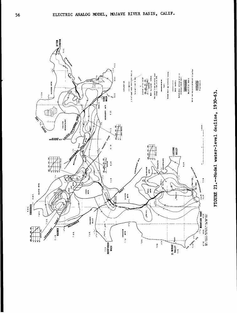
in

T D

H

BUCK

THOR

N W

ASH

M a M

O o C-H >.

V-

"'"

MOUN

TAIN

FR

ONT

'R.T

i,

net.

i s i

FIGU

RE 21

. Mo

del

water-level

decline, 19

30-6

3.


ir 9961

1961

/.SB I

E£61

6Z61

30VJ«nS QNV1 M0139 '133J Nl 'H31VM 01 HldBQ

(0JC8-MCO

2t3JE1

in ,en o

1 3E

5961

1961

/.SB I

£561

5*61

IfrBl

/.EBl

EE61

6Z81

4Ju0) rH0) CO

CM CM

W

O

i i

30VJ«nS QNVl M0139 133J Nl 'H31VM 01 HldBO


MODEL PREDICTIONS AND RESULTS

The purpose of the analog model is to predict water-level trends to the year 2000, based on assumed hydrologic conditions and pumping of ground water at rates equal to and 20 percent higher than the pumping rate for the verified period (1960-63). The basin was initially programed for no recharge from the mountain area, the minor tributaries, or the Mojave River. The next program consisted of recharge to the aquifer from the Mojave River under average flow conditions (1931-65), wet or high flow conditions (1937-46), and dry or low flow conditions (1947-65) with the actual and proposed pumping. Additional uses of the model included the prediction of the drawdown at a hypothetical well field pumping 10,000 acre-feet of water in a 4-month period and the effects of adding imported California Aqueduct water to the Mojave River for conveyance to other parts of the basin.

The model response has confirmed the concept that the Mojave River is the primary source of recharge to the basin, particularly within 1 mile of the river channel. Much of the runoff from the San Bernardino Mountains to the desert basin occurs during periods of low flow, and therefore most of the recharge to the aquifer infiltrates upstream from Barstow. The Mojave River at Barstow received only 27 percent of the total volume of water that entered the basin at The Forks (1931-68). Generally, less water is available downstream from Barstow and the influence of the river as a source of recharge diminishes. However, during high floodflows, water is available for aquifer recharge in the lower part of the basin to the Calico-Newberry fault. Downstream from the fault, aquifer storage is small; at Camp Cady ground water rises to the surface in the river channel. From Camp Cady to Afton pumpage and water-level declines are minimal.

Except in the Hinkley Valley area, historical water-level data from 1930 to 1963 show that declines are generally not excessive with respect to the saturated aquifer thickness. Model results to the year 2000 show that the projected water-level declines in most areas are not critical or excessive, and in many areas closely approximate straight-line extrapolation of the historical data.

The model results indicate that the geologic boundaries of the basin have considerable influence on the response of the system when stressed. In parts of the basin, impermeable mountains and older alluvium of low permeability act as boundaries and decrease the cross-sectional area of the permeable river alluvium. The water in storage in the river alluvium in those locations is much less than where the aquifer is wider and thicker. Thus, any input or output of water from the river alluvium is reflected by large water-level fluctuations.

The model indicated that such geohydrologic boundary conditions were prevalent along the Mojave River from Victorville to Hodge, and from Barstow to Daggett. In the upstream reach of the river, from Victorville to Hodge, water flows throughout the year. Long-term water-level declines are less than 5 feet. Without the continual recharge of water to the narrow, highly

MODEL PREDICTIONS AND RESULTS 59

permeable aquifer, water levels would decline rapidly. Conversely, when floods move down the river, water levels rise rapidly, frequently as much as several feet. As of 1970 floodflows had little influence on the aquifer in this reach because water levels were close to the land surface. The lower half of the reach does not have perennial flow in the river and depends on floodflow to recharge the aquifer adjacent to the river. This reach of the river is just downstream from perennial flow and less than 40 miles from the source of the recharge at The Forks. Snowmelt or minor floods supply streamflow in this reach, and the water table fluctuates accordingly.

The reach of the river from Barstow to Daggett is farther downstream from the source of recharge, and here the Mojave River flows only during floods. Thus, in extended droughts, water levels in wells in this reach decline rapidly. Sporadic floods, large enough to reach Barstow, are necessary to raise the water levels several feet and replenish the water pumped out in the intervening years. Future population increases and industrial development in the Barstow complex will result in greater withdrawals of water from the aquifer and intensify the water-level declines when river recharge is not available.

Downstream from Daggett the permeable aquifer widens. Short-term effects of infrequent streamflow and recharge to the aquifer are usually not transmitted more than a mile from the river. The water table does not fluctuate greatly because the aquifer has large storage capacity. However, ground-water underflow and recharge from the Barstow area eventually move downgradient to supplement the ground-water supply in the lower part of the basin.

Modeling the Mojave River is difficult because of the short-term storms and floods and the variable antecedent soil moisture of the river channel. For the verification period of the model 9 1930-63, the average flow of the Mojave River for 1931-65 was programed as shown in table 1. This is feasible because the long-term model water-level changes are being matched with the historical data from the physical system. Short-term water-level fluctuations due to recharge from high flows in the river are not important in this case because these single flood events are integrated into the long-term average.

Predictions of water-level changes, particularly near the Mojave River, are largely dependent on future flow conditions in the river. Accordingly, it was assumed that future flow will be the same as the average flow for 1931-65. However, future climatic conditions may be wetter or drier than the historical long-term average. Short-term, single flood events cannot be anticipated, but average flow during historical wet and dry climatic periods can be estimated. Flows simulating excessively wet and dry periods were programed into the model to study the water-level changes occurring under these conditions. Generally, the model data indicate a continual lowering of water levels. The rate of decline varied near the river depending on the quantity of recharge from streamflow, amount of pumping, and the configuration of the nearby impermeable boundaries.


No Aquifer Recharge, Storage Depletion, 1930-63

A theoretical water-level change map was made for 1930-63 assuming that all water pumped was derived from ground water in storage. No recharge to the aquifer was simulated in the model from the Mojave River, adjacent mountains, or side tributaries. The storage-depletion map (fig. 23) when compared with the actual water-level change for the same period (fig. 20) shows the importance of the Mojave River as a source of recharge to the basin, particularly upstream from Hodge. The greatest difference in water-level change between the two maps is along the river downstream from Victorville to about Hodge. Without perennial river recharge, maximum water-level declines from 1930 to 1963 would have been more than 40 feet, whereas, actual water- level declines were less than 5 feet.

Upstream from Victorville to the headwaters of the Mojave River in the San Bernardino Mountains, water-level declines under storage-depletion conditions are not substantially greater than under actual hydrologic conditions. This indicates that river recharge beneath the shallow channel alluvium in this reach is not as much as might be expected, even though this reach has the greatest potential for recharge because of storm runoff from the nearby mountains. The model results helped substantiate the theory, based on meager geohydrologic data, that a lack of continuity exists between the Mojave River and the deeper aquifer. (See sections on the Mojave River and verification of the model.)

In the lower part of the basin downstream from Barstow, the actual water- level declines are less than shown in the storage-depletion analysis. This difference in water-level change reflects the effects of recharge from the Mojave River to the aquifer. Short periods of floodflow in the Mojave River are the only important source of recharge to the lower basin as only 27 percent of the streamflow that entered the basin at The Forks reached Barstow during 1931-68. Consequently, much of the water pumped out of the lower basin is derived from storage in the aquifer.

Water-level declines in the Harper Lake area are similar to those determined by the storage-depletion study. This area is essentially isolated hydrologically from the Mojave River, and recharge from underflow is therefore minor.


c o<U

9̂

o4J (0

62

T3 (U Pu

oM00

C CO

0) 00

g<u

envD

oCO

<u3rH U (U

(U T3

I

en

O


Basin-Wide Water-Level Changes with Extremes in Mojave River Flow, 1930-2000

Prediction of future water-level changes caused by pumping is one of the main uses of the model. The most significant hydrologic variables in the basin are the distribution and quantity of inducible recharge from the Mojave River and the pumpage from wells. Future variations in these parameters are unknown, but limits can be estimated by an analysis of the historical data and then simulated with the model. Accordingly, model response was measured to the year 2000 under average and extreme flow conditions in the Mojave River.

The pumpage in the basin was simulated in the model to the year 2000, in some cases by simply projecting the 1960-63 rate. In other model runs, the 1960-63 pumping rate was increased by 20 percent throughout the basin. Another variation was to adjust the future pumping in the Hinkley-Barstow and Victorville areas in anticipation of growth in population.

All measurements of water-level change on the model are based upon the assumption that steady-state flow existed in the system prior to 1930. Hence, most water-level decline maps have been referenced to the base year, 1930, such as 1930-70, 1930-80, 1930-90, and 1930-2000. In some cases, however, maps were prepared that showed water-level changes occurring during the intervals, such as 1970-2000. In addition to the water-level contour maps, hydrographs showing model response at 19 points throughout the basin were also prepared (table 8 and fig. 24).

The predicted changes in water levels from the model are based on available factual data and assumptions on estimated future conditions. Changing geohydrologic conditions such as climate, variations in distribution and density of economic growth, pumping patterns, streamflow, phreatophyte modification, changes in the proposed imported water program, and political, economic, and legal considerations can affect development of the basin and water use. However, the model is useful in appraising the range and limits of water-level change with time and is the most practical way to integrate the multiple causes and effects in the physical system.

Figure 25 shows the water-level declines from 1930-2000, based on historical consumptive-use pumping from 1930 to 1963, a 20-percent increase from the 1960-63 rate for the period 1964-2000, and average flow conditions in the Mojave River (table 8, model condition 3). The purpose of this map is to show the total water-level decline that can be expected in the basin to the year 2000. Part of these declines have occurred while the future declines were estimated from the model. Model condition 3 is useful in evaluating the water-level declines in relation to the total aquifer thickness. The permeable aquifer along the Mojave River yields most of the water. As much of this aquifer is only 100-200 feet thick, these declines are a significant part of the aquifer. Elsewhere in the basin the permeable part of the aquifer is much thicker and can accommodate greater water-level declines.


TABLE 8.-- Model predictions, 1930-2000

Water-level decline,

Node

FG-60

FC-72

EY-64

EQ-72

EM-56

DO-48

CU-52

BG-56

Verificationperiod 1930-63 1930-70

26 29293334

25 29293232

35 39424447

18 22 222424

2% 3333

3 3333

14 16202023

17 25252727

in feet

Predictions

1930-80

33303840

34333840

43405056

27 263033

3h3h3h4

4344

18172432

40404343

1930-90

36354246

37374349

45485562

31 303641

3%3h3%4

4344

20232839

50505757

c 1930-2000

38364652

42404755

49465770

34 334148

4345

43%4^§5

23203144

60607070

Model :ondition

1234

1234

1234

1 234

1234

1234

1234

1234


TABLE 8. Model predictions, 1930-2000 Continued

Water-level decline,

Verification Node period

1930-63

AU-48 32

CE-72 15

BS-76 44

CA-84 24

BW-96 17(Bar stow)

CA-120 19

CA-132 11

CE-144 10

in feet

Predictions

1930-70

44444848

20202122

47475152

303032 .34

21232427

24242628

15151617

13131313

1930-80

57576565

26242831

54516061

37304042

25103038

29273336

20202225

18181919

1930-90

69697878

32303641

60577072

43394953

27233447

34334043

25272833

23232424

1930-2000

79799292

36344349

66617982

48395560

29133854

39364550

30313540

27273131

Model

1234

1234

1234

1234

1234

1234

1234

1234


TABLE 8. Model predictions, 1930-2000 Continued

Water-level decline, in feet

Node

BS-144

BG-148

CE-160

Verification period1930-63 1930-70

7 9159

10

11^ 14141717

lh 9999

Predictions

1930-80

13121416

17202626

12121313

1930-90

17261922

20263232

14141617

Model condition*

1930-2000

20212328

23303738

16171920

1234

1234

1234

1 Model conditions: Verification period 1930-63 contains programed consumptive-use pumpage and average flow in the Mojave River at different sites. Predictions of water-level change from 1964-2000 are based on the following assumptions:

1. Pumping rate 1960-63 and average flow in Mojave River 1931-65 extended for 1964-2000.

2. Pumping rate for 1960-63 extended for 1964-2000 and flow in Mojave River programed as low or drought period (based on records 1947-65) and as high or wet period (based on records 1937-46). Under this condition, the low flow was programed for 1964-70 and 1980-90, and high flow was programed for 1970-80 and 1990-2000.

3. Same condition as 1 except 1960-63 basin pumping rate increased 20 percent for 1964-2000.

4. Pumping rate for 1960-63 increased 20 percent and extended for 1964-2000. Mojave River flow programed as low flow or drought period for 1964-2000.

T e

N.BU

CKTH

ORN

WAS

H

W O

H O o

o M pa en M 5=5 P M

'" "

M

OUNT

AIN

FRON

TR

I «

R.G

«.

R 5

«

FIGU

RE 25. Model w

ater-level decline, 1930-2000.


Declines are more than (1) 100 feet in Harper Lake, (2) 80 feet in Hinkley Valley, (3) 50 feet south of Apple Valley, (4) 45 feet at Daggett, (5) 35 feet at Bars tow, and (6) 45 feet north of the Mojave River in the lower basin. Minimum declines are at Victorville and north to Helendale; elsewhere development of pumping is minor.

Figure 26 shows the water-level declines estimated from 1970 to 1980, on the basis of historical consumptive-use pumping from 1930 to 1963, a 20-percent increase from the 1960-63 rate for 1964-80, and average flow conditions in the river. The purpose of this map is to show water-level declines that can be expected for a 10-year period in the future. The water- level trends continue downward with the largest declines generally adjacent to the Mojave River in the lower parts of the basin. Declines are more than 20 feet in Harper Lake, adjacent to the north side of the Lockhart fault, and 12 feet in Hinkley Valley, Apple Valley, and north of the Mojave River in the lower basin. Other areas of 5-10 feet of decline are Barstow, Daggett, Calico-Newberry fault area, Helendale, and Hesperia-Apple Valley. Minor declines of less than 5 feet occur from Victorville to Helendale, Adelanto, and near Afton.

Figure 27 shows the predicted water-level change from 1970 to 2000, based on the consumptive-use pumping rate of 1960-63 in most of the basin extended to the year 2000. In the Hinkley Valley-Barstow area and at Victorville future pumping was based on projected use. In the Barstow area pumping for domestic and industrial use is expected to increase as the area urbanizes and the population increases from 23,700 in 1965 to 219,000 in 2000. In this area (fig. 27) consumptive water use was computed to be 10,600 acre-feet per year in 1960-63, 11,000 in 1970, 15,000 in 1980, 21,300 in 1990, and 32,200 in 2000. On the basis of consumptive-use values of 40-50 percent, the 1960-63 water production was about 20,000-25,000 acre-feet per year. In Hinkley Valley, water use was expected to decrease because of reduction in agriculture and to stabilize at about 10,000-15,000 acre-feet per year of production.

In the Victorville area, most of the large water production is from wells adjacent to the Mojave River for agriculture. Future pumping will probably not increase from the 1960-63 rate. The reduction in water use by a decrease of agricultural land will be offset by an increase in water use for urbanization.

The predicted water-level changes for 1970-2000 under the above assumed conditions show major declines of more than 35 feet in Harper Lake, 35 feet at Barstow, 25 feet at Daggett, and 20 feet in Hinkley Valley. These water- level declines reflect regional water-level changes in the aquifer and not pumping levels in wells. Small declines occur from Victorville to Helendale and away from the Mojave River where pumping is minor.

oo

I. H

isto

rica

l puw

ait

1930

-63

1.

Futu

re

punp

ini,

!96<

-60.

as

sum

d 20

uticin

t in

crta

se

1980

-83

rate

P

M o H 5 O M

< W pa

txi

FIGU

RE 26

. Mo

del

water-level

decl

ine,

1970-80.


o o o

O 3

CM

O M ft,


All the preceding model runs were programed with the yearly extremes of high and low flow in the Mojave River averaged as a continuous flow rate for the period of record 1931-65. However, during these 35 years, wet and dry climatic periods have occurred, and streamflow was greatly above or below the long-term average. Analysis of the streamflow records indicates 1937-46 was wet with high average flow; whereas, 1947-65 was dry with low average flow. Accordingly, these extremes in flow were modeled to show the possible range in water-level changes caused by varied recharge from the Mojave River. For the model, the flow of the river for the future, 1964-2000, is assumed to be within these limits.

Figure 24 shows water-level change hydrographs of 19 selected nodes under two hydrologic conditions. One condition represents extremes in Mojave River flow. The low flow or drought condition was arbitrarily modeled for 1964-70 and 1980-90; the high flow or wet condition was modeled for 1970-80 and 1990-2000 (table 8, model condition 2). The future ground-water pumping was maintained at the 1960-63 rate. The second condition shown on the hydrograph represents effects of average flow in the river for 1931-65 and a 20-percent increase in basin pumping from the 1960-63 rate (table 8, model condition 3).

In addition, as a maximum limit of future water-level changes in the aquifer, a drought condition (Mojave River flow averaged for 1947-65 period) was programed from 1964-2000 with pumping 20 percent greater than the 1960-63 rate (table 8, model condition 4).

Effects of Pumping a Well Field

Industrial growth will probably increase in the Mojave River basin as the Los Angeles megalopolis becomes more densely populated and economically less favorable to industrial expansion. The advantages of piping imported water from the California Aqueduct to a plant site or pumping locally from the aquifer was studied by using the model. For example, a proposed industrial plant was assumed to require 30,000 acre-feet of water per year, with 100-percent consumptive use. The initial entitlement of imported water to the basin is about 10,000 acre-feet per year. If all this water were diverted to the plant, it would meet its requirements for only 4 months per year. This is equivalent to pumping an equal quantity of water from the aquifer for 4 months. The model was used to determine the configuration and depth of the drawdown cone in the aquifer if pumped at the rate of 10,000 acre-feet in 4 months (18,800 gpm) with no return to the system.

Two sites were chosen. The first site is 9 miles north of Victorville, adjacent to the area of perennial flow in the Mojave River, and the second site is 2 miles southeast of Yermo, adjacent to the normally dry Mojave River (fig. 28). The cone of depression caused by the pumping will be different at each location because of the varied geohydrologic conditions at each site. Also, the future water-level declines caused by the proposed well field and nearby pumping would have some influence on which site is preferable. Other considerations, such as the cost of land, labor costs, transportation, power, and operating costs, are not within the scope of this study.


The site north of Victorville was chosen for model analysis because of (1) its proximity to Victorville, (2) access to railway and highway facilities, (3) availability of water, and (4) high aquifer transmissivity. Replenishment or recharge conditions are favorable because of perennial flow in the Mojave River. The site is only 25 miles from The Forks where flow of the Mojave River enters the basin.

The geologic section across the river channel at the hypothetical well field shows the limited thickness and width of the permeable aquifer (fig. 28). The channel was eroded out of the older, poorly permeable sediments and refilled with the river alluvium of sand and gravel. Storage capacity of the aquifer is limited, so continual recharge from the river is necessary to maintain high water levels. Wells producing in this area are above average for the basin and should yield at least 2,000 gallons per minute. Nine wells, spaced 2,000 feet apart, are assumed to yield the necessary quantity of water (18,800 gpm). In the model these wells were grouped into four nodes, 4,000 feet apart.

Water-level predictions from the model were made under two hydrologic conditions, based on the quantity of flow in the Mojave River. One condition assumes average flow in the river (floodflow and ground-water discharge), and the other condition assumes base flow only (ground-water discharge) measured at the Victorville gage. Average flow past the gage for 1931-65 was 47,205 acre-feet per year, including base flow and floodflow, of which 16,440 acre-feet per year flowed past the downstream gage at Barstow. Thus, nearly 31,000 acre-feet per year of surface flow was available for aquifer recharge between Victorville and Barstow. The base flow at Victorville is about 21,000 acre-feet per year, and ceases as surface flow about 1 mile downstream from the proposed well field. The average flow in the river has more water available for recharge than the base flow because of floods.

Both stream conditions were modeled, and the water-level effects were measured at model node DO-48 (center of well field, fig. 28). The hydrograph shows the water-level decline at this node due to pumping from 1930-66, with the effects of the additional 4 months of pumping imposed on the system. The total decline was 22 feet under average flow in the Mojave River and 27 feet under base flow conditions, of which 19 feet and 24 feet, respectively, were due to short-term pumping only.

Figure 28 shows the drawdown cone due to the pumping only under base flow conditions in the river. Maximum declines of 20-25 feet occur at the center of the well field. The hydrologic influence of the eastern boundary of poorly permeable sediments is reflected in greater water-level declines east of the river. If 30,000 acre-feet per year are required, the wells would have to pump continuously, so no recovery period is possible.

The site southeast of Yerao, in the lower Mojave River basin, was chosen because (1) the area has high aquifer transmissivity; (2) it is isolated from large-scale pumping, particularly the military complex at Daggett and Yerao; (3) the aquifer is wide and deep; (4) it is adjacent to the Mojave River, a source of recharge from infrequent floods; and (5) it is at the lower end of the flow system in the basin.


Geohydrologic conditions differ here from the upstream site as indicated by a comparison of the drawdown cones. The alluvial aquifer is 5 miles wider and hundreds of feet thicker. Recharge potential is less in comparison with the upstream site, because the Mojave River is dry except during infrequent floods. Well yields may be smaller, requiring more wells to pump the required quantity of water.

The geologic section across the valley shows a large alluvial basin, bounded on the sides by the impermeable Calico and Newberry Mountains (fig. 28)o A vast quantity of water is stored in the surrounding aquifer with only the Calico-Newberry fault, 1 mile east, impeding flow. Long-term water- level declines are minimal because local withdrawals are small compared with the water stored in the aquifer. Assuming that wells in this area should yield about 1,000 gallons per minute, 19 wells, spaced 2,000 feet apart, are required to supply 18,800 gpma Wells of larger yield would reduce the total number of wells needed,, In the model these wells were grouped into eight nodes, 2,000 to 4,000 feet apart. The regional water-level decline at the downstream site for 1930-66 was 11-15 feet. The hydrograph of model node BX-132 (fig. 28) shows 12 feet of decline for this 37-year period. The additional 4 months of pumping causes an additional 18 feet of decline.

The cone of depression about the well field represents only the effects of a well field pumping for a period of 4 months. The decline lines are generally concentric about the well field, although the Calico-Newberry fault has a minor influence on water levels. The fault boundary would increase water-level declines locally west of the fault if the pumping time was lengthened. Maximum decline is about 18 feet in the eastern part of the well field. Wells would have no time to recover if 30,000 acre-feet per year is required at this site for the industrial plant.

Analysis of the hypothetical well field sites indicates that sustained well yields north of Victorville are largely dependent on continual streamflow, as the storage capacity of the permeable alluvium is not large. If the river ceases to be a source of recharge, this part of the basin could have the largest water-level declines (fig. 22). Any large withdrawals of ground water in this reach would reduce the quantity of recharge available downstream. The most important factor at this site is the availability of continuous streamflow for recharge to the aquifer.

The pumping at the site east of Yermo would not affect the water levels in the upper, middle, and parts of the lower basin. Most of the pumped water would be derived locally from the water stored in the aquifer. This site is in the lower part of the basin and depends on infrequent floodflow to recharge the aquifer. Without additional supplemental water, discharge would exceed recharge, and water levels would continue to decline. Because the transmissivity and storage coefficients are high in this area, continued pumping would cause a larger and larger cone of depression without excessive lowering of water levels in the well field area.


Effects of Artificial Recharge on River System

Detailed geohydrologic studies indicate that supplemental water is required if the basin is to fulfill its potential future growth. In 1963 the California Department of Water Resources and the Mojave Water Agency signed a contract for a maximum entitlement of 44,000 acre-feet of water per year imported through the California Aqueduct. The contract was amended in 1964 increasing the maximum amount of delivered water to 50,800 acre-feet per year. Table 9 shows the annual imported water entitlement from 1972 through 1990. By 1972 the East Branch of the aqueduct and the Cedar Springs Reservoir will be completed, and water will be available for distribution and use (fig. 29).

TABLE 9. Annual imported water entitlements, California Water Plan, 1972-90

Entitlement in ,j j Discharge

Year amended contract ,-,.<- ,\, j- *.\ (cubic feet per second)

__________________(acre-feet)_____________________________________________

1972 8,400 11.51973 10,700 14.51974 13,100 18.01975 15,400 21.0

1976 17,800 24.51977 20,200 27.51978 22,500 31.01979 24,900 34.01980 27,200 37.5

1981 29,600 40.51982 31,900 43.51983 34,300 47.01984 36,700 50.51985 39,000 53.5

1986 41,400 56.51987 43,700 60.01988 46,000 63.01989 48,500 66.51990 50,800 69.5


The distribution of imported water from the California Aqueduct is of major concern to the Mojave Water Agency. The aqueduct crosses the upper Mojave basin north of Phelan, and parallels the mountains toward Cedar Springs Reservoir, 5 miles upstream from The Forks on the West Fork of the Mojave River (fig. 29). Possible methods of distributing the water throughout the Mojave River basin include pipelines, canals, or using the Mojave River as a natural conveyance system. An economical method of conveying the water to the Mojave River is by a diversion gate at turnout 3 to an unnamed wash, tributary to the river about 3 miles north of The Forks. The desirability of any of these methods is not in the scope of this study.

If the water is distributed by pipeline or canal, and then recharged into the aquifer anywhere in the basin, the effects on the physical system could easily be determined from the model. The model was used to predict the effects of the Mojave River as a conduit system, on the basis of several assumptions. Generally, using the river to distribute the imported water at the low continuous rates would not benefit the lower part of the basin except during floods. The river channel is highly permeable, and water losses or recharge to the aquifer would be high in the upper reaches.

The agency must determine where and how to introduce the imported water into the total water-supply system of the basin. Engineering studies in 1965 indicated three alternatives for delivering imported water: pipeline, canal, and the natural channel of the Mojave River. Preliminary studies by Koebig and Koebig, Inc. (1965) showed the following relative cost comparison between the alternative plans.

Relative cost comparison between alternative plans 1 3 2_, and 3

Alternative plan

1 (Pipeline)2 (Canal)3 (River)

Construction cost

HighMediumLow

Project cost

HighMediumLow

Average annual cost

Capital

HighMediumLow

Maintenance and operation

Low MediumMedium HighHigh Low

The relatively low cost of using the Mojave River as a distribution system for the imported water directed the agency's attention to pursue this plan. This plan raises many questions concerning the monitoring of the water flow, its effect on quality, which part of the river system is benefited, and losses to phreatophytes.


The major question regarding this plan was how far downstream the imported water would be conveyed in the usually dry channel of the Mojave River. The concern of the agency was whether or not any water would reach the lower basin. In the model, it is easy to simulate recharge at discrete locations along the river and record the water-level change with time. This method of artificial recharge will only affect the water table directly beneath the river at these locations and those adjacent to it. Other areas would have to be recharged by constructing conveyance systems. On the other hand, it is more difficult to simulate with the model the distance surface water will flow in the river.

Determining how far the imported water will move downstream by using the model is based on many assumptions and conditions. These include antecedent soil-moisture conditions in the river channel, depth to water beneath the river, effects of phreatophytes, evaporation from the water surface, amount and distribution of pumping along the river, and most important, the infiltration rate of the aquifer. A logical way to move imported water to the lower basin is to release it during floodflow. Caution must be used so imported water is not recharged if flow should occur at Afton. Without the benefit of floodflow, the rate of imported water to be released is small, ranging from 11.5 cfs (cubic feet per second), or 8,400 acre-feet, in 1972 to a maximum of 69.5 cfs, or 50,800 acre-feet, in 1990.

Previous studies indicated that this method of moving water downstream is questionable because of the high permeability of the river channel in the upper basins and the low rate of surface flow for recharge. However, any recharge to the upper basin will eventually result in more water available downstream as infrequent floodflows will lose less water upstream.

Surface flow can move tens of miles in hours, wheareas ground-water movement through the aquifer may take years. A way to use the river as a natural pipeline to move water downstream is to raise the water table beneath the river channel to the land surface. Then flow will occur in the river. A water-level mound must be developed beneath the river in the aquifer. After being established, it must be maintained along the river. The rate of movement of water from the mound is controlled by the gradient or head difference and the transmissivity of the aquifer.

The sections of the Mojave River conducive to natural recharge are directly related to the different hydrologic characteristics of the river, separately modeled as reaches Q1-Q13 (fig. 15). Emphasis has been placed on the low flow characteristics of the river channel in attempting to evaluate the benefits to be derived from using the imported water for recharge purposes.


Along the river from The Forks northward for several miles the ability of the aquifer to transmit water is restricted because of sediments of low permeability below 100-150 feet. In the Victorville area, perennial streamflow for 15 miles has saturated the aquifer beneath the river. Thus, much of the river from The Forks to 5 miles south of Helendale is not amenable to increased recharge under the present pumping regimen. The reach from the end of flowing water south of Helendale to the Calico-Newberry fault is conducive to recharge, particularly the Hinkley-Barstow reaches. Downstream from the Calico-Newberry fault, development is minor with little justification for recharging with the expensive imported water. Therefore, potential recharge areas in the river ares (1) Turnout 3 to the western part of Apple Valley, (2) Helendale to Hodge, (3) Hodge to Barstow, and (4) Barstow to the Calico-Newberry fault.

To simulate stream infiltration on the model, diodes were used to limit the electric current representing recharge of imported water. Where the depth to the water table in the aquifer adjacent to the river was similar, several nodes were grouped to represent 3-10 miles of the river channel. In the first section of the river, the maximum recharge available filled the unsaturated zone between the water table and the land surface. When the water level reached the land surface, the recharge rate was reduced to maintain the head in the adjacent aquifer. Excess flow then passed downstream to the next section, which filled with the remaining quantity of water. This procedure was repeated in the model until the quantity of water available for recharge was depleted.

The depth of the unsaturated zone to be filled along the river ranged from zero (points of perennial streamflow) to more than 50 feet. The distance that the surface water moves downstream is controlled by the infiltration rate of the channel and the volume of unsaturated material to be filled. A lower infiltration rate requires more time to raise water levels beneath the channel; a higher infiltration rate requires less time. Regardless of the infiltration rate, the distance the water eventually moves downstream is about the same, assuming no change in the flow pattern of the ground-water mound due to new pumping.

On the model, recharge of imported water was assumed to start in 1972. A later starting date will not greatly change the results if water-level declines along the river are not excessive. The recharge was superimposed on the pumping development and other stresses in the system as defined previously. No short-term floods are assumed to move water downstream, as only the average flow in the river, 1931-65, was simulated. Recharge effects in the upper river reach, turnout 3 to the perennial flow in the river south of Victorville, were based on two geologic assumptions. First, it was assumed that a single aquifer exists in the area and that a direct hydraulic connection exists between the river and the deeper part of the aquifer. Recharge of 10,000 acre-feet per year (13-1/2 cfs) introduced at turnout 3 would take nearly 30 years to raise water levels high enough to cause surface flow in the river. During this time the water would be filling the large water-table depression caused by pumping adjacent to the river. This geologic hypothesis is not tenable, as field data indicate discontinuity between the river and the deeper aquifer, and floodflows do not fill the depression.


Second, it was assumed that no continuity exists between the river and the deeper aquifer. Furthermore it was assumed that the upper shallow zone is largely unchanged from natural conditions, a reasonable assumption because this reach has first opportunity for annual floodflow recharge. Under these conditions it would take at least 1 year at 10,000 acre-feet per year to fill the unsaturated zone in the upper shallow zone.

These two conditions probably represent the maximum and minimum response of the physical system to recharge if introduced at the rate of 10,000 acre-feet per year. The actual response would probably lie somewhere between the two extremes.

If 50,800 acre-feet per year (69-1/2 cfs) were recharged at river turnout 3, the flow would reach the phreatophytes and perennial flow 4 miles southeast of Victorville in less than 1 year,, Larger quantities of water move downstream faster, as evidenced by the measurements made in the field during flood flow

On the model, recharge was also introduced in the river channel about 5 miles south of Helendale at the rate of 10,000, 35,000, and 50,800 acre-feet per year. This point on the river was chosen as an input source of recharge because the perennial flow upstream would act as a conduit for moving water from the turnout. The effect of this recharge on the middle and lower basin was measured and is shown in figure 29.

At a rate of 10,000 acre-feet per year, the flow in the river would be maintained to about the Helendale fault area,, It would take 4 years to create a ground-water mound along the river channel and then about 10,000 acre-feet per year to maintain it.

At the rate of 35,000 acre-feet per year (48 cfs), the flow in the river would be maintained to a point about 3 miles west of Barstow. The water would reach this point in 14 years or by the year 1986. At the rate of 50,800 acre-feet per year, the surface flow would reach the Helendale fault in about half a year, Lockhart fault in 3-1/2 years, Barstow in 5 years, and Daggett in 10-1/2 years (mid-1982). After mid-1982, the surface flow would not move farther downstream because of increased pumping upstream. By 1990 the flow would still be at Daggett, but by 2000, the surface flow would have retreated to about the Waterman fault because of increased pumping at Barstow.


CONCLUSIONS

Analysis of the hydrologic system in the Mojave River basin, using the electric analog model, indicates that the long-term pumping is in excess of natural recharge, the water table is declining, and water stored in the aquifer is being depleted. The depletion is only 1-2 percent of the water in storage. Unfortunately, the depletion is not uniform throughout the basin but is localized because of pumping in the developed parts of the basin. Areas of maximum water-level declines are near Harper Lake, Hinkley, and Daggett, and east of Hesperia. The net depletion from 1930 to April 1969 is estimated at 700,000 acre-feet, with 525,000 acre-feet in the Mojave River area and 175,000 acre-feet in the Harper Lake area. The water-level declines and ground-water depletion from the basin are of concern to the Mojave Water Agency. This agency is responsible for replenishing the local water supplies. Accordingly, in 1972 supplemental water will be imported from the northern part of the State by the California Aqueduct. The initial annual entitlement is 8,400 acre-feet and increases to 50,800 acre-feet by 1990.

The model analysis was planned to help predict the water-level changes because of future pumping under prolonged conditions of average and extreme flows in the Mojave River, and the feasibility of using the natural river channel for transporting imported water downstream to the lower basins. The analog model indicates that the water-level declines to the year 2000 are approximately straight-line projections of the documented decline from 1930 to 1963. These projections are based on average flow (1931-65) in the Mojave River.

Wet and dry climatic periods result in extremes of flow in the river and different rates of water-level change (table 8). Surface flow in the Mojave River accounts for about 80 percent of the recharge to the basin. About 85 percent of the average flow (1931-68) entering the basin at The Forks remains upstream from Afton. Generally, less water becomes available downstream, and recharge from the river diminishes. Because the river channel is highly permeable and susceptible to recharge, low flows do not normally reach Barstow. Most of the recharge to the aquifer downstream from Barstow results from floods. From 1931 to 1968 only 27 percent of the water that entered the basin at The Forks reached Barstow most of it during the floods of 1932, 1937-38, 1941, 1943-46, 1952, 1958, and 1965-66.

An initial model study usually considers all facets of the geohydrologic regimen and reveals the importance of each individual factor. Later studies can be oriented to more detailed analysis of specific features of the system or particular segments of the basin. As more precise determinations of stream infiltration under varied soil-moisture conditions become available, the model can analyze in more detail the recharge capabilities of parts of the river system.

CONCLUSIONS 79

The model showed that the boundary conditions in the aquifer, such as faults, configuration of the basin, large variations in aquifer transmissivity, recharge areas, and pumping patterns, have a pronounced effect on water-level changes.

The upper basin is one of the best places to develop ground-water supplies because of its proximity to the main sources of recharge, the headwaters of the Mojave River, and runoff from the San Bernardino-San Gabriel Mountains. These areas account for about 97 percent of the basin recharge, with the upper basin getting first opportunity for replenishment. Perennial flow in the river for 15 miles in the Victorville area has stabilized water levels, and water-level declines are minimal. Results of the model studies, and subsequent analyses of well logs indicated a geohydrologic anomaly along the Mojave River near The Forks. A confining layer of low permeability hinders river recharge to the deeper aquifer, as evidenced by maximum declines in the deeper aquifer east of Hesperia.

A significant result of the model analyses is that the Hinkley-Barstow- Daggett area may experience water deficiencies at an earlier time than other parts of the basin unless floodflows are available to replenish the aquifer there. The reasons are greatly increased pumping predicted in the Barstow area and low storage capacity of the narrow channel aquifer between the mountains. The aquifer boundary and its small cross-sectional area cause large water-level fluctuations from pumping patterns or flood sequences. East of Daggett to Camp Cady minimal water-level declines are anticipated under current pumping patterns.

Model runs indicate that the natural Mojave River channel is not a satisfactory conduit for moving small quantities of imported water downstream to the lower basin. Major sections of the river are dry most of the year, and low flows are readily absorbed by the river-channel deposits upstream.

Under the present contract with the State, the flow rate of the imported water ranges from 11.5 to 69.5 cfs of continuous flow with no peaking privileges. The model indicates that the minimum flow of 11.5 cfs may eventually reach the Helendale-Hodge section of the river, and the maximum flow may ultimately extend to Daggett. On the basis of the analog model response, consideration should be given to receiving higher flow rates for shorter periods. The imported water could be placed in the river at the end of a flood using the wetbed channel as a conduit for moving supplemental water farther downstream faster.

This analog study simulates the ground-water flow system in the aquifer and future water-level declines under various hydrologic assumptions. It does not describe or analyze the quality of the water in the basin. The next step may be to incorporate this information into a water-quality study using modeling techniques. In the future, water quality may become more important than availability of water. The most recent studies discussing water quality as a part of the hydrologic system were by the California Department of Water Resources (1967) and by J. F. Mann, Jr. (written commun., 1970).


Information is needed on the water quality at various depths in the aquifer and on the mixing effects of good quality water of the Mojave River and the California Aqueduct with the ground water in the basin. The natural recycling of pumped water to and from the aquifer increases the salinity of the ground water. Continual water-level declines in the future will have an effect on water quality as the lower part of the alluvial aquifer contributes more water. Degradation of water quality should be discouraged. Pollution of ground-water systems generally takes years to become intolerable because of the slow rate of ground-water movement. Similarly, it takes years to remedy the situation and restore the aquifer to its original conditions.

The electric analog model can readily be adapted to new problems or to additional data that become available in the future. The present hydrologic problems may be superseded by more difficult problems in the future as the interrelated developments in the basin become more complex. This present model analysis should be regarded as an initial phase and not as a completion of all hydrologic study in the basin.

ELECTRIC ANALOG MODEL, MOJAVE RIVER BASIN, CALIF. 81

SELECTED REFERENCES

Bader, J. S., Page, R. W., and Dutcher, L. C., 1958, Data on water wells in the upper Mojave Valley area, San Bernardino County, California: U.S. Geol. Survey open-file rept., 238 p.

Blaney, H. F. , 1933, Consumptive use of water by native plants growing in moist areas in southern California, part I, in South Coastal Basin Investigation, Water losses under natural conditions: California Dept. Public Works, Bull. No. 44, 176 p.

Bowen, 0. E., Jr., 1954, Geology and mineral deposits of the Barstowquadrangle, San Bernardino County, California: California Div. Mines Bull. 165, 185 p.

Burnham, W. L., 1955, Data on water wells in Coyote, Cronise, Soda, and Silver Lake Valleys, San Bernardino County, California: U.S. Geol. Survey open-file rept., 48 p.

California Department of Engineering, 1918, Report on the utilization ofMojave River for irrigation in Victor Valley, California: Bull. 5, 93 p.

California Department of Public Health, 1966, Barstow ground water study: Report to Lahontan Regional Water Quality Control Board, 12 p.

California Department of Public Health and Department of Water Resources,1960, Ground water quality studies in Mojave River Valley in the vicinity of Barstow: Joint rept. by the two agencies, 60 p., 8 app.

California Department of Public Works, Division of Water Resources, 1934, Mojave River investigation: Bull. 47, 77 p.

____1952, Investigation of Mojave River, Barstow to Yermo: Rept. toLahontan Regional Water Pollution Control Board, 31 p.

California Department of Water Resources, 1965, Feasibility of serving the Mojave Water Agency from the State Water Project: Bull. 119-12, 77 p.

____1967, Mojave River ground-water basins investigation: Bull. 84, 151 p.

Cordes, E. H., Wall, J. R., and Moreland, J. A., 1966, Progress report onanalog model.construction, Orange County, California: U.S. Geol. Survey open-file rept., 16 p., app.

Dibble, E. F., 1967, Mojave Water Agency, Water production verification program: E. F. Dibble, Redlands, Calif., 39 p.


Dibblee, T. W., Jr., 1960, Geologic map of the Barstow quadrangle,San Bernardino County, California: U.S. Geol. Survey Mineral Inv. Field Studies Map MF-233, scale 1:62,500.

Dyer, H. B., Bader, J. S., Giessner, F. W., and others, 1963, Data on wells and springs in the lower Mojave Valley area, San Bernardino County, California: California Dept. Water Resources Bull. 91-10, 212 p.

Erie, L. J., French, 0. F., and Harris, Karl, 1965, Consumptive use of water by crops in Arizona: Arizona [University] Tech. Bull. 169, 44 p.

Ferris, J. G., Knowles, D. B., Brown, R. H., and Stallman, R. W., 1962, Theory of aquifer tests: U.S. Geol. Survey Water-Supply Paper 1536-E, 174 p.

Hardt, W. F., 1969, Mojave River basin ground-water recharge, with particular reference to the California floods of January and February 1969: U.S. Geol. Survey open-file rept., 13 p.

Hewett, D. F., 1954, General geology of the Mojave Desert region, California in Geology of southern California: California Div. Mines Bull. 170, v. 1, chap. 2, item 1, p. 5-20.

Karplus, W. J., 1958, Analog simulation: New York, McGraw Hill Book Co., 434 p.

Kocher, A. E., and Cosby, S. W., 1924, Soil survey of the Victorville area, California: U.S. Dept. Agriculture, Bur. Soils, p. 623-672.

Koebig and Koebig, Inc., 1962, Mojave Water Agency supplemental water report, Appendixes A, B, C, D: 69 p., app.

____1965, Preliminary planning for Mojave Water Agency, alternate plans for distribution of imported water: H p.

Koehler, J. H., 1970, Water resources at Marine Corps Supply Center, Barstow, California, for the 1969 fiscal year: U.S. Geol. Survey open-file rept., 22 p.

Kunkel, Fred, 1956, Data on water wells in Cuddeback, Superior, and HarperValleys, San Bernardino County, California: U.S. Geol. Survey open-file rept., 73 p.

____1962, Reconnaissance of ground water in the western part of the Mojave Desert region, California: U.S. Geol. Survey Hydrol. Inv. Atlas HA-31.

McClelland, E. J., 1964, Aquifer-test compilation for the Mojave Desert region, California: U.S. Geol. Survey open-file rept., 47 p.

Meinzer, 0. E., 1923, Outline of ground-water hydrology: U.S. Geol. Survey Water-Supply Paper 494, 71 p.

SELECTED REFERENCES 83

Miller, G. A., 1969, Water resources of the Marine Corps Supply Center area, Barstow, California: U.S. Geol. Survey open-file rept., 51 p.

Moritz, E. A., 1952, Report on Victor project, California: U.S. Bur. Reclamation rept., 42 p.

Page, R. W., and Moyle, W. R., Jr., 1960, Data on water wells in theeastern part of the middle Mojave Valley area, San Bernardino County, California: California Dept. Water Resources Bull. 91-3, 223 p.

Page, R. W., Moyle, W. R., Jr., and Dutcher, L. C., 1960, Data on wells in the west part of the middle Mojave Valley area, San Bernardino County, California: California Dept. Water Resources Bull. 91-1, 126 p.

Patten, E. P., Jr., 1965, Design, construction, and use of electric analogmodels in Wood, L. A., and Gabrysch, R. K., Analog model study of ground water in the Houston District, Texas: Texas Water Comm. Bull. 6508, p. 41-60.

Skibitzke, H. E., 1960, Electronic computers as an aid to the analysis ofhydrologic problems: Gentbrugge, Belgium, Internat. Assoc. Sci.Hydrology, Comm. Subterranean Waters, Pub. 52, p. 347-358.

Slichter, C. S., 1905, Field measurements of the rate of movement ofunderground waters: U.S. Geol. Survey Water-Supply Paper 140, 122 p.

Storie, R. E., and Trussell, D. F., 1937, Soil survey of the Barstow area, California: U.S. Dept. Agriculture, Bur. Chemistry and Soils, 46 p.

Theis, C. V., 1935, The relation between the lowering of the piezometric surface and the rate and duration of discharge of a well using ground-water storage: Am. Geophys. Union Trans., p. 519-524.

Thomasson, H. G., Olmsted, F. H., and Le Roux, E. F., 1960, Geology, water resources, and usable ground-water storage capacity of part of Solano County, California: U.S. Geol. Survey Water-Supply Paper 1464, 693 p.

Thompson, D. G., 1929, The Mohave Desert region, California, a geographic,geologic, and hydrologic reconnaissance: U.S. Geol. Survey Water-Supply Paper 578, 759 p.

Thornthwaite, C. W., 1948, An approach toward a rational classification of climate: Geog. Rev., v. 38, no. 1, p. 55-94.

Troxell, H. C., and others, 1954, Hydrology of the San Bernardino andeastern San Gabriel Mountains, California: U.S. Geol. Survey Hydrol. Inv. Atlas HA-1, 13 sheets.


U.S. Bureau of Reclamation, 1967, Summary of phreatophyte ground-water use study along the Mojave River: U.S. Bur. Reclamation, San Bernardino, 12 p.

U.S. Department of Agriculture, Weather Bureau, 1916-1940, Climatological data.

U.S. Department of Commerce, Weather Bureau, 1940-1968, Climatological data.

U.S. Geological Survey, 1960, Compilation of records of surface waters of the United States through September 1950, part 10, The Great Basin: Water-Supply Paper 1314, 475 p.

____1963, Compilation of records of surface waters of the United States,October 1950 to September 1960, part 10, The Great Basin: Water-Supply Paper 1734, 311 p.

____1961-68, Water resources data for California, part 1, Surface water records, volume 1: Colorado River basin, Southern Great Basin, and Pacific Slope Basins, excluding Central Valley: U.S. Geol. Survey annual repts., 1961, 448 p.; 1962, 479 p.; 1963, 463 p.; 1964, 498 p.; 1965, 470 p.; 1966, 482 p.; 1967, 488 p.; 1968, 498 p.

Walton, W. C., and Prickett, T. A., 1963, Hydrogeologic electric analog computer: Am. Soc. Civil Engineers, Jour. Hydraulic^ Div., v. 89, no. HY6, Proc. Paper 3695, p. 67-91.

GPO 981-653

U.S. GEOLOGICAL SL'F.VEYPREPARED IN COOPERATION WITH THE MOJAVE WATER AGENCY,

MARINE CORPS SUPPLY CENTER, BAR TOW. AND GEORGE AIR FORCE BASE FIGURE 24

R.43 E.

CUDDEBACK

T.8 N.

BUCKTHORNi WASH

T.4 N.

BLACK MTN

/ Coyot e \ ALVORD MTN

S 'Harper '

CALICO

MOUNTAINS

- i 193D' 1950' 1970 1990

1970^ 1990 -10 ^ 1930 1950 \1970 1990 ^

1930 1950 1970 19900 - -»

(ANE ANEWBERRY MTS

rlelendale X _

EXPLANATIONSHADOW

T 7 N. MTN SILVER

MTN50 1970 1990

0EG-56

Kodal location of hydrograph Fault

Dashed where approximately located

DO-48Model hydrograph

Model boundaryVertical lines show time, in years; horizontal lines show change in water level, in feet, below 1930 level Dashed where recharge enters or

discharge leaves basinFAIR VIEW1930 1950 \ 197 ) 1990 0

Water-level change shown on hydrograph

Mojave Ri ver channel

Solid line indi cates perennial streamflow

MODEL ASSUMPTIONSC|y|_eg

1930 1950 1970 19900

I3430

MOUNTAINS1930 1950 1970 1990 1. Historical pumpage, 1930-63

2. Basin pumping, 1964-2000, increased 20-percent from 1960-63 rate

3. Average continuous flow in Mojave River, 1931-65

Phreatophytes

LUCERNE VALLEY

Water-level, change shown on hydrograph

MODEL ASSUMPTIONS

x-v x'lHE FORKS"

AFTON CANYON

T.5 N.

EL MIRAGE/ VALLEY ,'o ptf elan

12MILES

R.7 W.

117 30 ' MOUNTAIN FRONTR.6 W. R-5 W.

1. Basin pumping, 1964-2000, at 1960-63 rate except in Barstow area pumping based on projected use

2. Extremes in Mojave River flow, based on average streamflow: low flow. 1947-65; high flow, 1937-46

3. Programed in model for future as low flow, 1964-70, 1980-90; high flow, 1970-80, 1990-2000

HAP OF MOJAVE RIVER BASIN. CALIFORNIA. SHOWNG SELECTED MODEL HYDROGRAPHS. 1930-2000

IBnse from U.S. Geological Survey topographic map of Southern California. 1:500.000. 1953

U.S. GEOLOGICAL SURVEYPREPARED IN COOPERATION WITH THE MOJAVE WATER AGENCY,

MARINE CORPS SUPPLY CENTER, BARSTOW, AND GEORGE AIR FORCE BASE

72-157

FIGURE 28

'

R.43 E.

CUDDEBACK

T 8 N.

BUCKTHORN WASH

_____1_____________2 ___.pp$.__J/ £;L,

f.Coyo te :.\

T.11 N.

KRAMER

J - -r-?-

124 1128 132 \136 140

**"

Newber

40 44 48 52Drawdown cone, in feet, at end of 4 months pumping 10 000 acre-feet from nine wells for industrial use under base-flow conditions

Drawdown cone, in feet, nt end of 4 months pumping 10 COO acre-feet from 19 wells for proposed i nclust r i a I use

MOUNTAINS

.[ - ILL . .."'

LUCERNE VALLEY0 Hesperia j .-,,

ll

-^ THE FORKS

AFTON CANYON

EL MIRAGE; VALLEY ,'0 phelan

T.4 N.

124 128 132 136

Model nodal grid

Pum|)ing node

(open ci rjle, hydrograph of pumping node)

B -B 1

Geohydrologic p rofi le

Fault


Model boundary

Dashed where recharge enteis or di scharge I eaves basin

Ipil^^pgS^y:^:^:1:^:^:^:1:^:^:1:^1:1:-:-:

Mojavel River channel

Solid line indicates perennial streamflow

PhreatophytesT.3

R.7 W.

II7 ° 30 MOUNTAIN FRONT

R.6 W. R.5 W.

SR.4 W.

12 MILESR.3 i I i

MAP OF MOJAVE RIVER BASIN CALIFORNIA, SHOWING MODEL EFFECTS OF HIGH RATE. SHORT DURATION PUMPING

Base from U.S. Geological Survey topographic nap of Southern California, 1:500 000. 1953

U.S. GEOLOGICAL SURVEYPREPARED IN COOPERATION WITH THE HOJAVE WATER AGENCY.

MARINE CORPS SUPPLY CENTER, BARSTOW, AND GEORGE AIR FORCE BASE FIGURE 29.

R.43 E.

CUDDEBACK

T.8 N.

BUCKTHORN WASH

EL MIRAGE

MENLO

MAR 121974

/-- i -wf { .! <^.:; :" :S: :;:£. I {\ /Coyote^ | i

T.11 N.

KRAMER

CALICO

MOUNTAINS35 DO fc '________________^ ...

HINKLEY NYDROLDGIC PROFILE

-____1980 boundar » -._2000 ~- ~ NEWBERRY MTS

R.2 E.HELENOALE HYDROLDGIC PROFILE

SHADOW

T.7 N. MTN BARSTON HYDROLOGIC PROFILE

X

Distance wale? moves downstream at various recharge rates, at indicated time interval

Fault

Dashed rt.s.z approximately located

10,00fi 3:re-feet per year

35,000 scfR-feet per year

Model boundary

j__________I _______Basfcsd where recfiarge enters or

Q;sctiarge iesves basin

50.800 acre-feet per year

i>_____ ^

PnreatophytesLUCERNE VALLEY

HYOROLOGU PROFILE

»

Showing water-level cdanp^a, in feet, frsm 1530

Location of profile

Effects frra basin pumping

T.5 N.

Pojave River channel

Solid less indicates perennial streamftow

VALLEY i 0 Phelan

T.4 K. /

\

T.3 N>x 0 \^ 34 0 20\

AFTON ' CANYON

R.7 W.

MOUNTAINR.6 I. R.5 t

Effects from artificial recharge put in river at end of perennial Mojave River flow, west of Silver Mountain, at rate of 50.800 acre- feet per year starting 1972 BIth basin pumping

MODEL ASSUMPTIONS

1. Xittarical pumpsge, 1930-63

2. fat,tire pumping, 1264-2000, assumed at 115C-63 rate; except in Bars tow casaiex pumping based on projected use

3. A'terage flow in Mojave River. 1931-65

IHAP OF MOJ/WE RIVER BASIN, CALIFORNIA, SHOWING MODEL STUDY OF IMPORTED YIATER RECHARGE ON RIVER SYSTEM

fBaia from U.S. Geological Survey topograpnic map of Southern California, 1:500,000, 1953

C^od)

U.S. GEOLOGICAL SURVEYPREPARED IN COOPERATION WITH THE MOJAVE WATER AGENCY,

MARINE CORPS Si PLY CENTER, BARSTOW, AND GEORGE AIR FORCE BASE 72-157 FIGURE 8

R.43 E.

CUDDEBACK

T.B N.

BUCKTHORN WASH

MENLO PARK

-121974

f Coy o t e " -\

CALICO

MOUNTAINS

Change-:in

river storage Line of equal estimated transmi ssi vi ty.

in thousands of gallons per day per foot.

Fault


Numbers along faults are estirnatPd transmissivity across the fault, in thousands of gallons per day per foot Model Soundary

Dashed where recharge enters or di scharge leaves basin

Modeled as two aquifers, with transmissi vi ty shown, equally di vi ded

Mojave River channel

S=0-12Sto rage coefficient3« D 30f

MOUNTAINS

Numbeir refers to table 3LUCERNE

j VALLEYVALLEY /O ptelan

-' THE FORKS

AFTON CANYON

Solid line indicates perennial streamflow

Plireatopriytes

EL MIRAGE

R.7 -

117030 MOUNTAIN FRONTR.6 W. R-5 W. R.4 W. R.3 N.

MAP OF MOJAVE RIVER BASIN, CALIFORNIA. SHOWING AQUIFER TRANSMISSIVITY AND STORAGE COEFFICIENT

iBaie fron US Geological Sjrvey tonograpliic map of Southern California, 1:500.000. 1953

prepared in cooperation with the mojave water agency u.s. … · 2010-10-23 · water resources...

Documents