Architectural Design and User’s Guide to the GLASScientific Computer Facility – Science Support Functions

Version 1.0

Prepared by

Anita C. Brenner, John P. DiMarzio, and Ziporah Sidel

Raytheon ITSS, NASA/GSFC Code 971

Prepared forH. Jay Zwally and The GLAS Science Team

DateMay 31, 2001

2

Table of Contents PageTable of Contents Page ...................................................................................... 21.0 Scope of this Document............................................................................................. 32.0 Requirements ............................................................................................................ 5

2.1 mSCF requirements ............................................................................................... 52.2 Remote SCF Requirements.................................................................................... 5

3.0 Overview................................................................................................................... 54.0 Facility Description ................................................................................................... 6

4.1 Main SCF.............................................................................................................. 64.2 Remote SCFs......................................................................................................... 6

5.0 Architectural Design.................................................................................................. 85.1 Interface between the I-SIPS and the main SCF..................................................... 8

5.1.1 Subscriptions between the mSCF and the I-SIPS............................................. 95.1.2 Special Requests from the mSCF to the I-SIPS ............................................. 105.1.3 Quick Look Data Requests from mSCF to the I-SIPS ................................... 105.1.4 Science Team QA......................................................................................... 105.1.5 Level 3 and 4 products.................................................................................. 11

5.2 Interfaces between the main SCF and remote SCFs ............................................. 115.2.1 Data requests from the rSCFs to the mSCFs.................................................. 115.2.2 Level 1 and 2 Data Distribution .................................................................... 115.2.3 Data Issues and QA ...................................................................................... 125.2.4 Delivery of level 3 and 4 products from the remote SCFs to the main SCF. .. 135.2.5 Change requests for algorithm modifications for creation of level 1 and 2products................................................................................................................. 13

5.3 Data Management................................................................................................ 145.3.1 Product sets .................................................................................................. 145.3.2 Data Base Management System .................................................................... 17

5.3.2.1 DBMS Table Formats and Creation ....................................................... 185.4. Reference Orbit and Granule sub-setting software ............................................. 21

5.4.1 The reference orbit sub-setting software, orbselect........................................ 215.4.2 The granule sub-setting software, data_select and prod_create ...................... 22

5.5 Data Requests...................................................................................................... 235.5.1 Data Request Interface.................................................................................. 245.5.2 Data Request Management System .............................................................. 26

5.5.2.1 Subscriptions ......................................................................................... 265.5.2.2 Special Requests from the rSCF to the mSCF......................................... 275.5.2.3 Quick Look Requests ............................................................................. 27

5.6 Data Visualization Software ................................................................................ 285.6.1 Visualization software requirements ............................................................. 285.6.2 Data Selection Interface ................................................................................ 29

5.7 Data Issues Forum .............................................................................................. 345.8 SCF internal Web Page........................................................................................ 34

6.0 User’s guides........................................................................................................... 356.1 Data Request GUI User’s guide for version 200105.0.......................................... 35

6.1.1 Subscriptions ................................................................................................ 366.1.2 Special Requests ........................................................................................... 40

3

6.1 Data Visualization User’s guide for version 200105.0 ......................................... 416.2.1 Select from Data Base................................................................................... 426.2.2 Select from specific data set option ............................................................... 476.2.3 Visualize the data.......................................................................................... 47

Appendix A - Definition of Orbit parameters: ............................................................... 59Appendix B – mysql data request tables ........................................................................ 60

1.0 Scope of this Document

Provide architectural design and users guides for all components of the science-supportfunctions of the GLAS SCF. This includes data management, data distribution, datavisualization, and a WEB page with up-to-date processing status and product-specificinformation.

The GLAS SCF is also the test bed for developing, maintaining, and testing the GLASscience algorithm software, and the host of the ICESat Science Investigator-ledProcessing System, the I-SIPS, and the Instrument Support Facility, ISF. The I-SIPSand ISF are not discussed here and are described in separate documentation. Everywherethat the main SCF is referred to in this document refers to the science support portion ofit located in room B209A of building 33 at GSFC and does not include the I-SIPS or theISF.

This document is intended to be used by users of the GLAS SCFs, (the science teammembers and their colleagues). Section 3 gives the user a general overview of thescience support functions. Section 4 provides a general conceptual knowledge of thefacilities. Section 5 presents the architectural design of the SCF support software andsection 6 gives the user’s guides for the individual components. Section 5 may be helpfulto understanding the user’s guides. Users who are only looking for how to run a specificcomponent on their machine can skip directly to the user guide for that component.Programmers who will be modifying and maintaining the code can use this document tounderstand conceptually what it is trying to do, however they should be using the detaildesign document to understand the code. The plan is to have the software installed byRITSS on the rSCFs. However a software installation guide will be delivered to each sitefor completeness.

The full complement of expected documentation of the SCF is summarized below:• Main SCF

o Architectural Design and User’s guide to the GLAS Scientific ComputerFacility – Science Support Functions (this document)

o Detail design document of each individual componento Installation guides for each individual component

• Interface Control Document between the I-SIPS and main SCF• I-SIPS

o Detail design document for the I-SIPS Science Data Management Systemo Procedure guide for the I-SIPS – operatorso User’s guide

4

• ISF - TBD

5

2.0 Requirements

The requirements can be broken up into mSCF and rSCF components. It is to beremembered that the mSCF serves functionally the same purpose as the rSCF for theproject scientist since his team is co-located with it at GSFC.

2.1 mSCF requirements

The basic requirements on the mSCF that are not levied on the rSCFs are as follows:1. Distribute GLAS standard products and appropriate geographic and/or temporal

sub-sets to the science team2. Provide a facility for development and maintenance of generalized GLAS analysis

and visualization tools that are distributed to the science team3. Maintain a bulletin board for science team comments on GLAS standard data

products, SCF-supplied software and algorithm feedback discussions.4. Maintain an issues page for GLAS standard data products that is accessible to

NSIDC5. Communicate science team QA of GLAS standard data products to the I-SIPS6. Create or receive level 3 and 4 products and distribute them to the I-SIPS7. Provide test bed for development and maintenance of GLAS science data

processing software8. Provide on-line storage of all GLAS level 2 and selected GLAS level 1 products9. Host a data base management system for the local data10. Provide GLAS science team with pertinent GLAS processing and product

information, including access to browse products

2.2 Remote SCF Requirements

Each remote SCF has the following requirements:1. Provide test bed for tuning of GLAS science algorithms2. Perform data analysis of GLAS data in the PIs area of expertise3. Provide on-line storage for the local GLAS data the specific PI is utilizing4. Host a data base management system for the local data5. Run software supplied by the mSCF in IDL, Fortran 90, or Unix scripts6. Communicate with the mSCF for data requests7. Communicate science QA to the mSCF8. Develop level 3 and 4 products

3.0 Overview

The mSCF is the distributor for all level 1 and 2 GLAS standard data products to theGLAS science team. The rSCFs obtain data by requesting it from the mSCF using theData Request Interface. The request is automatically emailed to the main SCF, where it isparsed and kept track of in the special request and subscription data bases. Distribution

6

to the remote rSCFs is done in product sets, which contain full granules or temporaland/or geographic subsets of the granules and associated tables for data basemanagement. The subsetting capability will allow science team members to store at theirremote SCFs only the portion of the data that satisfies their interests. Tools will besupplied with the data for the science team to QA the data, assess the accuracy andappropriateness of their processing algorithms, develop and test modifications to theprocessing algorithms, and produce publication ready plots of GLAS product output. AWeb page will be maintained at the main SCF for all team members to check processingstatus and view browse products from all GLAS level 1 and 2 granules, access ancillarydata sets, keep informed of GLAS operating conditions, and share results.

There are 15 level 1 and 2 GLAS standard products. These are produced by the I-SIPS ingranules as summarized in table 1. Each of these products has an associated browseproduct which consists of a set of web-browser viewable images from which the user candiscern the overall quality of the granule. The main SCF will receive on a subscriptionbasis from the I-SIPS all level 2 GLAS standard data products, GLA08-GLA15, the polargranules of the level 1 altimetry products, GLA01, GLA05, and GLA06, and browseproducts for all GLA01-GLA15. These subscription products will be kept on-line ondirect access disks and will be managed using a custom-built data base managementsystem. Science team data requests can be for any level 1 and 2 product. If the datafrom which the request must be filled does not reside at the main SCF then it will bepulled from the I-SIPS. An automatic interface will be used for this and should beinvisible to the science team member. The I-SIPS will maintain an archive of all GLASlevel 0, level 1, and level 2 products and ancillary data sets used to produce themthroughout the mission. GLA04 is not listed in table 1. It is a multi-file granule thatcontains SRS, GPS, and LPA information required by the UTCSR for calculating orbitsand attitude values. GLA04 is currently being provided directly to UTCSR by the I-SIPS and does not go through the main SCF.

4.0 Facility Description

This section describes the facilities at the mSCF and each of the rSCFs.

4.1 Main SCF

The GLAS mSCF consists of a redundant pair of UNIX servers and sufficient RAIDstorage for all GLAS level 2 and selected level 1a and 1b products. Figure 4.1 shows thecomponents of the mSCF.

4.2 Remote SCFs

The general configuration for the rSCFs is a UNIX server and sufficient RAID storagefor the GLAS products the PI associated with that rSCF wishes to analyze. The DLTauto changer is supplied for backup and exchange of data sets greater than 2 Gbytes insize. The DVD Figure 4.2 shows a diagram of the typical remote SCF configuration.

7

Figure 4.1 - Components of the Main SCF

.

8

Figure 4.2 Remote SCF Configuration

5.0 Architectural Design

This section describes the software that is being developed at the main SCF for thegeneral use of the science team. It consists of 8 subsystems:

1. The I-SIPS – mSCF interface2. mSCF-rSCF interfaces3. Data management4. Reference orbit and Granule sub-setting software5. Data requests6. Data Visualization Software7. Data Issues Forum8. Web page

5.1 Interface between the I-SIPS and the main SCF

The specifics of the interface hand shaking are defined in the I-SIPS – GLAS SCFInterface Control Document (Brenner et al 2001). There are 5 interfaces from thefunctional viewpoint.

1. Subscriptions for GLAS Standard Data Products and related files from the I-SIPSto the main SCF

2. mSCF Special requests for non-subscription GLAS Standard Data Products fromthe I-SIPS

3. mSCF Quick look data requests to the I-SIPS4. Science team QA results from the mSCF to the I-SIPS5. Processing status from the I-SIPS to the mSCF

9

5.1.1 Subscriptions between the mSCF and the I-SIPS

The main SCF will subscribe to the following from the I-SIPS:1. All granules of GLA08-GLA152. Polar granules of GLA01, GLA05, and GLA063. Browse products from all GLAS standard data products, GLA01 – GLA154. Bin/rev tables created from GLA05 and GLA07 (see section 5.3)5. Rev table in ASCII to include, revolution number, longitude of the ascending

node, pass id, and beginning time of the revolution6. Granule table information in ASCII (TBD We may not need this)7. Reference orbit table in ASCII8. Reference orbit track files

During normal processing, the first four items above will be sent as a package referred toas a product set. Each product set will contain the required files for 14-orbits of data.This is the granularity of the level 2 data sets. These will be sent automatically by the I-SIPS as soon as all the files that make up the package are completed. At the same timethe updated rev table information and updated granule table information ???TBD willalso be sent. The reference orbit table information and reference orbit track files will besent each time we enter a new reference orbit.

During reprocessing, any granules and associated browse products and bin/rev tables thatare remade that are normally under subscription will be sent. This may not include all thegranules listed above since partial reprocessing of only selected granules can be invoked.These will be sent in 14-orbit packages. The rev table will not be updated sincereprocessing will not alter it.

The distribution planner and database at the I-SIPS will contain the information as towhat the mSCF subscription consists of and how to package it. When each subscriptionis complete a distribution job will run at the I-SIPS to place the data sets in the mSCFdistribution cache on the I-SIPS. After all files in the product set have been placed in thecache the PDR will be put there containing the following information:

• Unique distribution ID assigned at the I-SIPS• Total number of files in the set• File names• File sizes and/or checksums

The mSCF will run a script regularly that looks for PDRs in this cache. When a PDR isfound it is ftp’d to the mSCF ingest cache and deleted from the I-SIPS cache. The fileslisted in the PDR are then ftp’d into the mSCF ingest cache. The file sizes and/orchecksums are checked and if correct, the file is then removed from the I-SIPS cache. Ifany problems exist then an email is sent to the I-SIPS operators explaining the problemand giving the unique distribution ID associated with the PDR.

10

5.1.2 Special Requests from the mSCF to the I-SIPS

Any product that an rSCF user requests that is not included in the subscriptions defined insection 5.1.1 will be considered a special request. This does not include requests forproducts that have not yet been processed at the I-SIPS, or for which the mSCF has notyet received because the 14-orbit package in still not finished. These conditions will fallin the quick look category discussed in section 5.1.3.

Special Requests will be sent to the I-SIPS with a unique special request ID and a specificpriority flag set at the mSCF. This flag sets the priority of the distribution job required tofill the special request at the I-SIPS. When the I-SIPS distribution job runs, it fills asmuch of the special request as it can placing the requested files and a PDR in the mSCFdistribution cache on the I-SIPS. The Product Delivery Record will contain

• Unique distribution ID assigned at the I-SIPS• Unique Request ID assigned at the mSCF• Total number of files in the set• File names• File sizes and/or checksum

If no files are produced, a PDR will be placed in the distribution cache with the SCFUnique Request ID, the I-SIPS-defined unique distribution ID, and 0 for the number offiles indicating that the request cannot be filled.

The mSCF will ingest the files into the ingest cache in the same manner as described forsubscriptions in section 5.1.1. The mSCF should then confirm the request was valid andresubmit or correct as necessary.

5.1.3 Quick Look Data Requests from mSCF to the I-SIPS

Quick look data requests are for data which has not yet been processed, either due toschedule restraints at the I-SIPS or because all required input data is not yet available.The request will require sign off by the TBD board who will also set the priority, sincethis affects processing at the I-SIPS. The mSCF will submit the request for quick lookdata in the same method as for special requests, except it will use a priority level thatforces data to be expedited. Based on this priority, the I-SIPS will force processing of therequested files out of order, using expedited data if necessary, or processing partialgranules if all input data does not exist. If a granule cannot be created, I-SIPS will keeptrying for 24 hrs. After 24 hrs, a PDR will be placed in the distribution cache with theSCF Unique Request ID and 0 for the number of files indicating that the request cannotbe filled. The mSCF should then confirm the request was valid and resubmit or correctas necessary. The rest of the transfer and ingestion process is the same as for specialrequests described in the previous section.

5.1.4 Science Team QA

11

The mSCF will send the I-SIPS updated granule-specific science Quality Assuranceinformation based on science team perusal of the data by creating a science QA updaterequest file and putting it and the accompanying PDR in the mSCF input cache on the I-SIPS. This QA update file will contain a list of granule names with the new value for thescience QA flag.

The I-SIPS will update its database and have an interface with NSIDC to update thegranule’s metadata.

5.1.5 Level 3 and 4 products

Level 3 and 4 products, created at or sent to the mSCF, will be delivered to the I-SIPS fordistribution to NSIDC. These will be placed in the mSCF ingest cache on the I-SIPS withan associated PDR and unique distribution ID. Any problems the I-SIPS has ingestingthese files is to be communicated to the mSCF via email with the unique distribution ID.The mSCF will then retransmit the files as necessary.

5.2 Interfaces between the main SCF and remote SCFs

Five functional interchanges have been defined between the mSCF and the rSCFs;1. data requests from the remote SCFs to the main SCFs2. data distribution from the main SCF to the remote SCFs for level 1 and 2 GLAS

standard products and subsets thereof,3. data issues and QA4. delivery of TBD level 3 and 4 products from the rSCFs to the mSCF,5. change requests for algorithm modifications for creation of level 1 and 2 products

5.2.1 Data requests from the rSCFs to the mSCFs

All requests for data from the science team originate at the rSCFs using the Data RequestInterface installed on the remote site computer. Only the mSCF can request or receivedata from the I-SIPS so the rSCFs have to send all requests to the mSCF. The DataRequest Interface sends email with the specifics of the request to the mSCF where it isautomatically parsed, kept track of in a database, and assigned a unique ID. Anacknowledgement of the request is then emailed back to the rSCF with the unique ID andan interpreted summary of the request. There are three distinct types of requests;subscriptions, special requests, and quick look requests as discussed in section 5.5. Afterthe request is filled, the files created from the request are placed in the rSCF-specificdistribution cache as explained in the next section.

5.2.2 Level 1 and 2 Data Distribution

A separate distribution cache for each rSCF will be maintained at the mSCF. Theinstitution named on the data request submittal will determine in which distribution cachethe results are placed. The output of all requests will be placed in this cache as a set of

12

files and a Product Delivery Record (PDR). The PDR will be an ASCII file in the formatdescribed in table 2

Table 2 – Format of PDR for transmittal of data from mSCF to rSCF –Capital letters denote keywords and must be typed as shown, lines are terminated by asemicolon.Line # Keyword Value1 REQUEST_ID= unique request ID assigned at the mSCF2 TIME_STAMP= yymmddhhmmss of time subscription was filled (executed)3 TOTAL_FILE_COUNT= Number of files in this delivery 1-99994 OBJECT= FILE_GROUP5 OBJECT= FILE_SPEC6 FILE_ID= Name of file7 FILE_SIZE= Size of file in bytes (<2GB)8 END_OBJECT= FILE_SPEC9-N Repeat of lines 5-8 for each file In the deliveryN+1 END_OBJECT= FILE_GROUP

A data ingest script will be delivered to the rSCF to check the mSCF output cache, readany PDRs, download all files listed in the PDR to a local rSCF data directory using ftp,check file names and sizes against the PDR, and remove the downloaded files andassociated PDR from the distribution cache. This script should be run periodically by therSCF.

After TBD hrs, if the data has not been pulled by the rSCF, it will be downloaded to tapeor CD-ROM, removed from the cache, and shipped to the remote SCF. This is put in asa safe hold only and is not supposed to be the normal mode of running. Each rSCFshould be running its data ingest script automatically at least daily.

5.2.3 Data Issues and QA

A data issues forum will be maintained at the mSCF. This will be maintained in abulletin board format with search and cataloguing capabilities and accessible to the rSCFsfrom the GLAS SCF internal web page. This gives the science team members an easyway of communicating any issues they have with the data or SCF supplied software tothe rest of the science team and the mSCF support staff.

GLAS is also required to release a public GLAS data issues page that is linked intoNSIDC and made available to all users. This issues page is ultimately the responsibilityof the science team. The mSCF support staff will maintain this page, however it is up tothe science team to assure the information represents their issues. Development andoperational versions of the issues page will be maintained. The science team will benotified by email every time the development version is modified and given 48 workinghrs to respond with modification requests. After this waiting period, and any requestedmodifications have been incorporated, the development version will be presented to the

13

TBD board and after sign-off be moved to the operational version which will be given toNSIDC for public access.

The SCFs are also responsible for science QA of the I-SIPS granules. The science teamcannot inspect every granule. However, it is the responsibility of each PI to assure byspot-checking that the parameters they are responsible for have reasonable values and toevaluate the quality of the parameters calculated from their algorithm. This is especiallyimportant after new algorithms are implemented. This science quality is carried on themetadata of each granule at NSIDC and in the I-SIPS database. A science quality updateGUI will be assessable from the internal SCF web page with which to update the definedquality values. A comments section will be included for justification of the change in thequality flag. This comments section will be linked to the bulletin board, such that itautomatically creates a bulletin board message. A request for change in a quality flagwill be presented to the TBD board for signoff and then sent to the I-SIPS forimplementation.

5.2.4 Delivery of level 3 and 4 products from the remote SCFs to the main SCF.

The science team is responsible for creation of GLAS level 3 and 4 products. They caneither be created at the remote SCF or the software can be placed on the main SCF or theI-SIPS and the products can be created there. The products will then be sent to I-SIPS forreformatting if necessary and distribution to NSIDC. The exact interface for this is TBD.

5.2.5 Change requests for algorithm modifications for creation of level 1 and 2products.

There will be a configuration control board (CCB) consisting of TBD that must okayalgorithm modifications. A formal change request system will be used, accessible fromthe internal mSCF web site. The science team member will fill out this request form online to request specific algorithm modifications. These modifications will be categorizedby product and/or specific sets of parameters. Team members will be asked to sign up forcategories for which they want to be notified of requested modifications. All teammembers will have access to the change request data base and will be able to peruse anypart of it they wish. Team members who sign up in a specific category will be notified byemail of any requested modifications in that category and allowed to comment beforeCCB action is taken. Both modifications that require coding changes or changes to theancillary input files (i.e. waveform parameterization input) must be submitted to the CCBsince both code and ancillary files used for level 1 and 2 are under configurationmanagement (CM). The CCB will decide what requests are accepted, what version ofthe software they will be put in, and when that version will go operational.

Table 1 - GLAS Standard Data Products

ProductID

Granule sizeMbytes

Product Name GLAS/ICESat–Level..)

Primary Intended Users

14

GLA01 ~ _ orbit 34 MB L1A Global Altimetry I-SIPS, Science team,altimeter scientists

GLA02 2 orbits 703 MB L1A Global Atmosphere I-SIPS, Science team GLA03 2 orbits 13 MB L1A Global Engineering I-SIPS, Instrument team GLA05 ~ _ orbit 21 MB L1B Global Waveform-

based Range Corrections I-SIPS, Science team,

altimeter scientists GLA06 ~ _ orbit 9 MB L1B Global Elevations I-SIPS, Science team,

altimeter scientists GLA07 2 orbits 828 MB L1B Global Backscatter I-SIPS, Lidar scientists,

Science team GLA08 14 orbits 2 MB L2 Global PBL & Elev.

Aerosol Layer Heights I-SIPS, Atmospheric

scientists GLA09 14 orbits 81 MB L2 Global Cloud Heights

for Multi-layer Clouds I-SIPS, Atmospheric

scientists GLA10 14 orbits 301 MB L2 Global Aerosol

Vertical Structure I-SIPS, Atmospheric

scientists GLA11 14 orbits 12 MB L2 Global Thin Cloud/

Aerosol Optical Depths I-SIPS, Atmospheric

scientists GLA12 14 orbits 49 MB L2 Polar Ice Sheet

Altimetry Ice scientists

GLA13 14 orbits 22 MB L2 Sea Ice Altimetry Ice scientists GLA14 14 orbits 273 MB L2 Global Land Surface

Altimetry Land scientists and

topographic mapping GLA15 14 orbits 240 MB L2 Ocean Altimetry Ice and Ocean scientists

5.3 Data Management

At the main and remote SCFs data will be kept in product sets. All sub-sets of productswill be created in the same format as the products themselves. Sub-setting here refers toselecting records by time and/or location, but not picking out specific parameters fromthe product.

5.3.1 Product sets

Product sets consist of• One or more GLAS standard products – GLA01-GLA15• Browse products for each of the GLAS standard products• Data Base Management System tables

o One Pass table for each GLAS standard product file in the product seto One unique record index table for each GLAS standard product file in the

product seto One or more bin tableso A georeference table for each bin table

Product sets at the mSCF - These will span a time period equal to the time of the level 2granules, which span 14 revolutions of data. All product files in the mSCF product setsare the original files as sent by the I-SIPS (non sub-sets). Each mSCF product set willcontain the following:

• GLAS standard data products subscribed to from the I-SIPS

15

o 28 polar granules (segments 1 and 3) each for GLA01, GLA05, andGLA06

o 1 14-revolution granule each for GLA08 through GLA15• Browse products for all GLAS standard products in this time frame – this includes

the granules not contained in the product set such as the equatorial granules(segments 2 and 4) for GLA01, GLA05, and GLA06; and GLA02 and GLA07.

• Data base tableso One Pass table for each GLAS standard product file in the product seto Two bin tables –one made from all GLA05 granules created at the I-SIPS

and one made from all GLA07 granules created at the I-SIPSo Two georeference tables, one for each bin tableo One unique record index table for each GLAS standard product file in the

product set

When new granules are received, the bin table files at the mSCF will be searched todetermine if a product set already exists for this 14-revolution time frame.If the product set does not exist it will be assigned a unique mSCF PID, the files from theingest cache to the product_set cache renaming them appropriately and appropriate tablescreated. If product set exists, we find the unique mSCF PID, move the files from theinput cache to the product_set cache renaming them appropriately, create new pass andunique record index tables for each new GLAS standard product granule received,replace the georeference and bin tables and run outstanding subscriptions against the newdata only. Browse products will be staged to the mSCF internal home page.

File names at the mSCF-The names of the files at the mSCF will be dependent on the I-SIPS naming convention. The I-SIPS file naming convention is as follows:

HHHxx_mmm_prkk_ccc_tttt_s_nn_ff.eeewhere

• HHH=Type identification-GLA, ANC,SCF,BRW,QAP,ING,…• xx = Type ID number• mmm = Release number for process that created the product.• p =Repeat ground track phase• r= Reference orbit number• kk=instance # incremented every time we enter a different reference orbit• ccc = Cycle (000-999)• tttt = Track (0000-2600)• s = Segment, (0=none, 1-4 correspond to 50° lat/lon breaks)• nn = granule version number (the number of times this granule is created for a

specific release)• ff =file type. (numerical, CCB assigned for multiple files as needed for data of

same time period for a specific HHHxx, i.e. multi-file granule)• eee = file extension-dat, scf, hdf, eds, met….

NOTE – This naming convention is currently under discussion, to allow all products sentto NSIDC to begin with the GLA or ANC type identification and use an extra extension to

16

define browse or Quality Assurance files. If the I-SIPS naming convention is changedthen the mSCF naming convention will change accordingly

For files that are exact duplicates of the I-SIPS files, i.e. the GLAS standard data productsand the browse products, the name will be the I-SIPS name with PID appended.(currently the extension eee is removed first, but depending on the note above it may needto remain)Where

• PID is the unique product set ID of the format Pnnnn where nnnn is a uniquenumber identifying that product set formed by incrementing the previous productset PID by one.

The Data base tables will be named as follows:• pass table - same as the corresponding GLAS standard data product name with the

GLA changed to PS and appended with PID where

vv is the version number, it starts out at 00 and increments by 1 everytimethe table is recreated for this product set

• Unique_rec_index table, same as the corresponding GLAS standard data productname with the GLA changed to UR and appended with PID

• Bin tables – BNx_prkk_ccc_tttt.ID_vv where

prkk_ccc_tttt come from the corresponding GLAS standard data productnamex =A for the bin table is to be used for the altimetry productsx = L for the bin table to be used for the lidar products

• Georeference table - GRx_prkk_ccc_tttt.PID_vv

Product sets at the rSCF-Product sets for each rSCF will be created from subscriptionsand special requests submitted from that rSCF. Each product set will contain

• One file for each different GLAS standard data product selected in the sameformat as that produced at the ISIPs but with only the records within the requestedtime and region

• A browse product for each GLAS standard product file in the product set• One Pass table for each GLAS standard product file in the product set• Up to Two bin tables – one each for LIDAR and altimetry products• A georeference tables corresponding to each bin table• One unique record index table for each GLAS standard product file in the

product set

The bin table(s) and corresponding georeference table(s) will always be created from thealtimeter and lidar data sets in the product set that have the most covereage since thesetables are not associated with a specific physical file but correspond to the whole timeperiod.

17

When new versions of data are received from the I-SIPS, the subscription table will besearched for any subscriptions against this data. These subscriptions will be executedagainst the new version and the new files added to the original product set with theversion number updated. Associated Browse products, pass and unique record indextables will be remade and the creation table updated. Software supplied to the rSCF thatuse these product sets will always use the latest version by default.

The rSCF file naming convention will be as follows:

• GLAS standard data products - GLAxx_yymmddhh_tiiii.nnnn_vv• Browse products – BRxx_ yymmddhh_tiiii.nnnn_ff_vv• Pass table - PS_ yymmddhh_tiiii.nnnn_vv• Bin table - BN_yymmddhh_tiiii.nnnn_vv• Georeference table - GR_ yymmddhh_tiiii.nnnn_vv• Unique_rec_index table, URxx_ yymmddhh_tiiii.nnnn_vv

Wherexx = GLAS Standard data product number (1-15)yymmddhh – date of first data in data sett=type of request; s for subscription, r for special requestiiii is the subscription number or special request numbernnnn – unique product set ID number, PIDff – file number to account for multi-file browse productsvv- version of this file starting at 00

Header records in each GLAS standard data product file will list the specific inputparameters used to fill the request, and the I-SIPS input files used so the user can keeptrack of what I-SIPS versions went into each data set. 5.3.2 Data Base Management System

The DBMS does not use special COTS software but consists of a set of tables that areassociated with each data file or set of data files in a product set. The purpose of the datamanagement system is to allow one to create sub-sets of the GLAS standard dataproducts by directly accessing the records that fall within the temporal span and/orgeographic region requested for the subset instead of reading through all the datasequentially. This allows for creating subsets of the original GLAS product granulesefficiently, since the entire granule need not be read to determine the specific recordsrequired. This design is based on the DBMS in use at GSFC for the polar ice radaraltimetry data. The only real requirement for this type of system is that the data filesmust be direct access files. For GLAS we also make use of the fact that each data recordin every granule contains the unique record index assigned when processing the level 0data. This unique record index is assigned for every 1 second frame of data and is afunction of the time on the level 0 data. Since it exists on every product, one can use it tocorrelate data across the products.

18

To allow geographic sub-setting, the world is divided into a set of bins. This georeferencebin configuration selected for GLAS is defined in table 2. Given this information, the binnumbers included in any latitude/longitude defined rectangular region can be analyticallycalculated.

Table 2 Georeference Bin Configuration for GLAS

One bin and georeference tables could theoretically be created for each product set. Todo this would require having a product; whether it consists of 1, 7, or 56 granules; thatcontains the time and a precise geographic location for all data on every product in thisproduct set. This eliminates GLA01-GLA03 because the geographic locations on theseproducts is not precise and is estimated from the predicted orbit. We also do not haveany single standard product that is guaranteed to contain a complete set of times forwhich we could have either LIDAR and/or altimetry data. The LIDAR telemetry comeson different APID files than the altimetry and each goes through different processingscenarios on board the satellite. This means that we could end up with time periods forwhich we have LIDAR data and no altimetry and vice versa. Therefore two sets of binand georeference tables for each 14-orbit product set at the mSCF are created; one fromGLA07 for LIDAR products, and one from GLA05 for altimetry products. Theseproducts both have records at the high resolution of 1 sec and geographic locations basedon the precision orbit.

For the rSCFs, we have no control over what products they select for their product set.Using the same logic as above, we need to a bin and georeference table separately for theLIDAR and altimetry products respectively. The LIDAR georeference and bin tables,will be created from GLA07 if it is present, otherwise we will use this hierarchy; GLA08,GLA09, GLA10, GLA11, GLA02. The altimeter georeference and bin tables will becreated from GLA05 or GLA06 if present. If only the level 2 regional products areselected then it will be created from merging the information on all the selected level 2products. GLA01 will be used to create these tables only if it is the only altimeterproduct in the set.

5.3.2.1 DBMS Table Formats and Creation

The beginning of each table consists of header records consisting of “keyword=value”strings in ASCII. The header records are followed by fixed length binary data records.

Beginning Latitude -90.0°NBeginning Longitude 0.0°EEnding Latitude 90.0°NEnding Longitude 360.0°EWidth of bins in Latitude° 1.0Width of bins in Longitude° 1.0

19

The first two records of each file are:

RECL=NNUMHEAD=M

Where N is the integer record length of the data records and M is the number of“keyword=value” header records.

Reading the first 7 bytes of the file gives the record length of all records. The first datarecord number can be calculated from the NUMHEAD variable which gives the numberof header records of RECL length in bytes. More keywords may follow that are table-specific. Following the header records are the data records defined below

Bin Table-This table defines which bins each data set traverses and the unique recordnumbers within the data set that go through that bin. It is a direct access file that has onerecord for each instance that a pass enters and leaves a bin. The bin tables are 24bytesrecords, the data records are described in table 3.

Table 3 – Bin table data record format

Bytes Type of variable Description1-4 I*4 Georeference bin number5-16 Char*12 Pass ID (prkkccctttt)17-20 I*4 Unique record index of first record on this pass

that traverses this bin21-24 I*4 Unique record index of the last record on this

pass that traverses this bin

The data records in the bin table file are sorted primarily by bin number, secondarily bypass number, and finally by beginning unique record index.

To create the bin/rev directory table, a Fortran 90 program, mkbinrev, is supplied thatreads sequentially all the data in the product set for that specific product. As each datarecord is read, the geographic bin corresponding to the latitude and longitude on thatrecord is calculated using the geographic bin configuration. The program keeps track ofthe first unique record number and the last unique record number for each bin and outputsa record to a scratch file every time the bin number changes. This scratch file is thensorted first by bin, then pass ID within the bin and lastly by unique record index withineach pass within the bin. The sorted file is then the bin directory table.

Georeference Table - This is a directory of the bin table that allows direct access to thestart of each bin the bin table. There is one georeference table for each bin table.The georeference directory tables are direct access files of 12 bytes record length.consisting of : geographic bin number, beginning data record number within the bin/revtable for this bin, and the ending data record number within the bin/rev table for this bin -each a 4 byte integer field. The georeference table is created from the bin table using the

20

Fortran 90 program, mkgeo. Note that the size of both these tables is dependent on thegeographic bin resolution and not on the resolution of the data.

Table 4– Georeference table data record format

Bytes Type of variable Description1-4 I*4 Georeference bin number5-8 I*4 beginning data record number within the bin/

table for this bin,9-12 I*4 ending data record number within the bin table

for this bin

Unique Record Index Table -This is a table that allows one to calculate the data recordswithin a file that correspond to specific unique record index numbers. One of these isrequired for each GLAS standard product file (GLA01-GLA15) in the product set. This isa direct access file of either 20 or 24 byte records. The extra 4 bytes are required for thetable for GLA01 in order to specify waveform record mode. Data records are defined intable 5.

Table 5– Unique Record Index table data record format

Bytes Type of variable Description1-4 I*4 Beginning unique record number5-8 I*4 Ending unique record number,9-16 R*8 UTC time of the beginning unique record

number in seconds relative to noon, January 1,2000

17-20 I*4 The data record number within this file thatcorresponds to the beginning unique recordnumber – the first data record is number 1(header records do not affect this number)

21-24 I*4 Waveform record mode (for GLA01 only)

One data record is written every time there is a break in unique record index in the file orfor GLA01, a record also has to be written every time the waveform record modechanges. Note that for the granules with a record time span of 1 second, the uniquerecord index will change by approximately 10 between contiguous records, for thegranules with a record time span of 4 seconds; the unique record index will change byapproximately 40 between contiguous records.

Pass Table – This table defines the passes present in the product set. One pass table isrequired for each GLAS Standard Product in the Product set. The pass table is a directaccess file of 20 byte records. The format of the data records is given in table 6.

Table 6– Pass table data record format

Bytes Type of variable Description

21

1-4 I*4 Reference orbit designator - prkk5-8 I*4 Cycle number -ccc9-12 I*4 Track number - tttt13-16 I*4 Beginning unique record number of a

contiguous span of data17-20 I*4 Ending unique record number of a contiguous

span of data

The pass table will have one record for every contiguous set of data for a specific pass.

5.4. Reference Orbit and Granule sub-setting software

Two packages of sub-setting software are used; one for geographic sub-setting of thereference orbit and one for geographic and temporal sub-setting of the data granules.

5.4.1 The reference orbit sub-setting software, orbselect.

Orbselect is a set of scripts and Fortran 90 code that determines the tracks and portionsthereof of a reference orbit that traverse a specific geographic region. The data requestinterface and the front end of the data visualization interface use orbselect to showprojected GLAS coverage on a map. Given a geographic region defined by a rectangle inlatitude and longitude, orbselect outputs a list of GLAS tracks that go through thatrectangle and the indices within those tracks. A separate list is obtained for eachreference orbit (i.e. 8-day and 183-day).

where• Reference orbit – an orbit which is maintained to within 1 km cross-track on the

ground• Track – one orbit revolution within a reference orbit, starting and ending at the

ascending node• Track Index – index within the track latitude and longitude arrays that define a

unique ground location

The Reference orbit ground track file is defined from the reference orbit ephemeredesdistributed by UTCSR. It is interpolated to 1 sec intervals along the track and stored as adirect access binary file where each record has arrays giving the latitude and longitudecoordinates for one track in the format defined in table 7.

Table 7 – Reference orbit ground track file

Record # bytes Variabletype

Description

1 1-23204 R*4array(5801)

Array of latitude values for each second alongtrack 1 – at end of array extra values are filledwith –999.0

23205-46408 R*4array(5801)

Array of longitude values for each second alongtrack 1 – at end of array extra values are filledwith –999.0

22

array(5801)

track 1 – at end of array extra values are filledwith –999.0

46409-46412 R*4 Deltat; time between values in the above arrays(nominally 1 sec)

2-n Same as above for tracks 2-n, 8- day orbit has 119 tracks, 183-day orbit has2723 tracks

Bin and georeference tables are created for the two reference orbit ground track filessimilar to the bin and georeference tables that are created for each data product set of dataas explained in section 5.3.2. Instead of listing the beginning and end unique recordnumbers that traverse each bin, the track number and beginning and ending 1 sec indiceswithin the track are listed in the bin table.

Given a geographic region defined as rectangle in latitude and longitude, first thegeographic bins contained in that region is calculated analytically using the georeferencebin configuration presented in section 5.3.2. The georeference and bin tables areaccessed to determine what tracks (and portions thereof) traverse the bins selected.

Now we know what tracks go through the enlarged geographic region and which portionsof each of them. This only gives this information to the precision of the geographic binconfiguration. To get rid of the false positives, the latitude and longitudes are read fromthe reference orbit ground track files for the tracks and indices selected and checkedagainst the selected region to output a refined list of tracks and indices. The output is thensorted primarily by track number and secondarily by index within the track.

5.4.2 The granule sub-setting software, data_select and prod_create

The granule sub-setting software requires as input

• The product sets from which to create the sub-setted products• Which GLAS standard products are requested, any or all of GLA01-03, GLA05-

15.• A region of interest defined as a rectangular region in latitude and longitude• A time span – optional

A set of Fortran 90 programs and scripts is supplied that accomplishes the following

1. Calculates the geographic bin numbers of all bins included within the requestedregion.

2. Calculates the pass span(s) for all passes included if a temporal sub-setting isrequired – see Appendix A for definition of pass

3. Accesses the georeference and the bin/rev directory tables for all product sets thatare input to this request and stores the sets of unique record index ranges that arerequired to fill the request.

23

4. Accesses for every granule for each product requested the unique record indextables and outputs a set of REQ files, one per type of standard data produce(GLA01, GLA02, …). Each data record in these REQ files contains the name ofthe product granule, a contiguous unique record index range, the correspondinggranule data record number range, and the pass id for the data that will satisfy therequest. There can be multiple records that have the same product granule name ifmore than one contiguous unique record index range is required for any granule

5. The REQ files are then read by another Fortran 90 program, prod_create, thatreads the input data granules, accesses the records required and does a furthercheck that the latitude, longitude and time on the data record is within the usersub-set requirement. The output of this program is one file for every GLASstandard product type requested with only the data requested. These files arewritten in the exact same format at the GLAS standard product granules. ForGLA01, 02, and 03 granules that contain predicted latitude and longitudelocations, all data within the geographic bins on the REQ files will be selected.

5.5 Data Requests

The only way the rSCFs receive GLAS data is by requesting it from the mSCF. A DataRequest Interface is provided on each rSCF and is to be used to initiate all data requests.There are three types of requests; subscriptions, special requests, and quick look requests.

Subscriptions are to be submitted to the mSCF for standing orders. Subscriptions willbe automatically executed every time the mSCF receives a new product set from the I-SIPS. Not all executions will create output, since not all geographic regions or time spanswill be covered in the 14 revolutions of data. In normal mode, each time a subscription isexecuted one product set will be created if data exists within the subscription constraints.If any one file in this data set would exceed 2 Gbytes in size, then the subscription will besplit by time to create multiple product sets.

A special request is a one-time request. Special requests will be executed on all productsets that exist at the time the request is received. One product set will be output with allthe data unless any one file would exceed 2 Gbytes in size. If so, the special request willbe split by time and multiple product sets created.

A quick look request is the tool the rSCF uses for requesting special processing at the I-SIPS. These requests must be approved by and given a priority by the special requestboard (details TBD). There are two types of quick look data that can be produced. Typeone is when the I-SIPS has all the required input files but for some reason or other has notyet processed the data. This could occur during reprocessing where the priorities were notset in line with the science team member requesting this data, or if during normalprocessing something occurred to get I-SIPS off schedule. For this type of data theoutput products will be of the same quality as if the data had been processed in sequence.

Type two is when all of the input files are not available and processing the data wouldresult in some of the output parameters being undefined or of lower quality than normal.

24

One situation this can occur under is if the team member is requesting processing of level1b and 2 data before the precision orbit and attitude files are ready. The scienceprocessing software, GSAS, can create the level 1b and 2 products using the predictedorbit. When this is done, however, the attitude information is not used at all andgeolocation is accomplished assuming a nadir-pointing laser.

When the main SCF runs a subscription or an rSCF special request, the mSCF firstchecks if all files required to fill the request reside at the mSCF. If they do not, then aspecial request is sent to the I-SIPS for these granules as explained in section 5.1.2.Whether the data resides locally at the mSCF or only at the I-SIPS should be transparentto the rSCF user. The only affect this will have on the user is that it will take longer tofill their request.

5.5.1 Data Request Interface

The data request GUI allows the user to select ICESat products by region, time, and/orset of tracks. The most restrictive information will be used - for example, if the userselects a time span or region and a set of tracks, he or she will receive only the subset ofthe tracks that are within the time span or the region. The GUI is set up to show theground tracks for both the 8-day and 183-day reference orbits whether processed or not.This is so that the requestor can put in a subscription for data that will be processed in thefuture. A list showing the processing status is also presented for user informationpurposes only.

There is an interface window from which the user selects what type of request this is;subscription, special request or quick look request. The only difference between a specialrequest and a quick look request is that the user will be asked to supply justification forthe quick look request. Subscription type requests allow the user to input more than onetime span for several years to allow for seasonal selection of a region over the missionlifetime.

The user will then see a data request interface which he/she uses to feel out the request.This main interface can bring up a map display that visually shows the user the GLASground tracks on a world map and/or overlaid on a digital elevation model and allows forinteractive mouse selection of the area of interest. There is also the option for plottinguser-defined locations from a file on the map so one can see where their specific area ofinterest lies with respect to the GLAS reference groundtracks. All selections made in themap display can be inherited by the main interface. However, the user can completelyfill out a request without ever accessing the map interface.

The main interface provides the following information and input options:• A Help button that displays a text file with general information on this display• ? buttons that display text files giving specific information on selected options• A Data Product Menu for choosing which GLAS standard products are requested• Text-input rectangular region selection in latitude and longitude• Time span selections

25

o Beginning and end time span (just 1 set) for special requests or quick lookrequests

o Set of time spans for subscriptions to allow choosing of seasonal data overmultiple years

• Lists of passes that traverse selected regiono One list of tracks for each reference orbito For each reference orbit

user can select all tracks, select a subset, select cycles, and resetselection

see a list of tracks that have already been processed as help to user• Target of Opportunity link to list track, date, and location of all targets of

opportunity in ICESat event log• Option to save request parameters so they can be reloaded to initialize the

interface for future requests• Option to initialize the interface using a saved set of request parameters• Options to input requestor’s institute and name• Summary of request at any time with push of a button• Option to submit request• Reset and exit options• Access to the map display that shows GLAS ground track coverage on maps

The map display provides the following information and input options:• Help button that displays a text file with general information on this display• ? buttons that display text files with specific information on selected options• Option to select general region; world, Antarctica or Greenland at the push of a

button• Arctic and Antarctic projected in polar stereographic projection• Option to display either 8-day or 183-day reference orbit ground tracks on map• Option to zoom map to change region selected and see detail of coverage• Option to change back to general region selected after zooming• Text input rectangular region selection in latitude and longitude correlated with

zoom and map selection• Gives list of all tracks in region for reference orbit selected. User can select one or

more individual tracks which are highlighted on the map. Option to load selectedtrack list into main window for filling of request.

• Option to plot map as either a flat continental outline or shaded-surface DigitalElevation Model

• Option to display only a given number of tracks at one time, show number oftracks left to display in region and display next set of tracks

The data request program uses the reference orbit subsetting software, orbselect which isa combination for Fortran 90 code and scripts to determine the reference orbit groundtracks. Note all ground tracks are plotted from the reference orbit and not from the data,which means that the laser is assumed to be nadir pointing.

26

The user’s guide in section 6.1 gives specifics on how to run the data request interface.

5.5.2 Data Request Management System

There will be shareware software used, mysql, to keep track of user’s data requests anddistribution. In this RDBMS, the following information will be maintained:

User- Information• User number – assigned by mSCF• User name• Institute name• User contact info – email, phone, fax, address

Subscription and Special Request input parameters• Time/pass span• Region latitude and longitude limits• A unique subscription or special request ID, siiiii or riiiii respectively• User number associated with the request• Which GLAS standard data products are requested

Distribution Information• Special request or subscription unique ID• PID span of the main SCF product sets used to fill the request (For subscriptions

this will only be one number, for special requests several main SCF product setscould be used)

• Date and time request filled• Time span of the data sent• Name and size of each file sent ( include output product set ID, PID)

5.5.2.1 Subscriptions

Subscriptions are handled as follows:

1. The information from the subscription email submitted using the Data RequestInterface is inserted into the mysql data base tables.

2. Every time a PDR is processed from the I-SIPS, if the keywords indicates it is asubscription then the time/pass spans of the product sets received are checkedagainst all subscriptions in the mysql subscription table.

3. A list is created of all granules required for each subscription that falls within thistime/pass span of the newly received data.

4. If any granules are required from the I-SIPS because they are not part of themSCF-I-SIPS subscription then

a. A special request is sent to the I-SIPS for these granules with an mSCFassigned ID

27

b. The mSCF ingest queue is checked regularly for receipt of the PDR andgranules that fill this special request by checking for the mSCF assignedID in the PDR

c. The files listed in the PDR are copied to a temporary data cache wherethey are checked for completeness against the PDR and the PDR and filesare removed from the ingest cache

5. The subscriptions are run inputting to data_select all product_sets required fromboth the temporary data cache and the product_set data cache

6. A PID is assigned to each product set created7. How do we account for reprocessed data where we want to add it to an existing

PID?8. Browse products, georeference, bin, unique record index and pass tables are

created9. The distribution table is updated10. Completed product sets and associated PDR are placed in the appropriate rSCF

distribution cache(s)

If a subscription is submitted covering a time span for which data already has beenprocessed, then it will be treated as a special request for the already processed portion ofthe time span and then as a subscription for the remaining portion of the time span.

5.5.2.2 Special Requests from the rSCF to the mSCF

1. The special request input is inserted into the mysql data base.2. A script is run to determine what I-SIPS granules are required to fill this request.

All granules that have been processed by the I-SIPS are checkedThe rest of the procedure is the same as for subscriptions in the previous section exceptthat if the special request results in no output, a PDR will still be placed in the rSCFdistribution cache, with no files listed, to indicate to the rSCF that the special request wasexecuted but no data existed to fill it.

5.5.2.3 Quick Look Requests

Quick look requests from the rSCF to the mSCF will be handled as follows:1. The mSCF will check the I-SIPS processing status to see if any data required to

fill this request has already been processed.2. If any data for this request has already been processed then the mSCF will create

a special request for the rSCF for creating a product set from the data that hasalready been processed, fill that request, and place the resultant PDRs and productset files in the rSCF distribution cache. An email will be sent to the rSCFexplaining that the quick look request has been split into a special request andquick look request and the corresponding unique request IDs so the rSCF cantrack it.

28

3. A request to fill the quick look portion of the request will then be sent to the TBDboard for permission and priority level. If permission is denied then the rSCF willbe notified by email of the denial and the reason.

4. If the board approves, a quick look request will be sent to the I-SIPS and insertedin the mSCF Data Request Management System.

5. I-SIPS processes the required granules and places the resultant PDR and granulesin the mSCF distribution cache on the I-SIPS. (see section 5.1.3)

5.6 Data Visualization Software

This software is written in IDL, but uses some Fortran 90 executables and shell scripts toallow the science team to visualize pertinent parameters of the GLAS standard dataproducts. This software is designed to allow the scientists to check out the performanceof their algorithms, understand the information on the individual products, and compareparameters across the elevation region 2 products. It should be useable as a first step inanalyzing the data.

5.6.1 Visualization software requirements

The requirements will be broken down into two sets; set 1 will be those requirementsplanned to be implemented by launch, and set 2 will be those requirements to beimplemented as data becomes available, and the need arises. The requirements that areplanned to be implemented at launch are as follows.

1. Displays in graphical form pertinent parameters from level 1 and 2 elevation andLIDAR products (GLA01-02, GLA05-15)

2. Allow user to select which data to visualize in one of two ways using a GUIa. By product type, time, pass id, and/or geographic region

i. shows ground tracks of available data on map over DigitalElevation Model (DEM) to aid in selection

ii. Lists all products available iii. Lists passes in region and time span selected

b. By selecting specific product files local to their SCF i. allow user to input multiple files from any one product set ii. allow user to input any file in GLAS standard product format

3. User can select a combination of any of the products to visualize together4. Displays pertinent parameters of selected data in appropriate graphical form with

the capability of creating a postscript file from any plotting windowa. Default plot parameters based on actual datab. User-controlled plot parameters to create publication quality plots

5. Runs on mSCF with access to all on-line data6. Runs on rSCFs with access to all product sets local to the specific rSCF

Requirements that are desired to be implemented after launch are

1. Add the engineering product GLA03 as one of the available products

29

2. Capability to input ancillary data and display with GLAS data3. Capability to display higher level GLAS products4. New requirements levied by the science team

5.6.2 Data Selection Interface

The main window will allow the user to either select data by region, time, and/or passspan or to input specific data files. All data to be visualized must be in the data directorythat will default to the designed directory or the user can specifically define. If the userwishes to look at a specific set of files another window will be displayed where the usercan input specific files, no more than one for any GLAS standard product type. Whencombining files from different product types, they must all be from the same product setor cover the same time span. This option allows the user to create their own standardproduct as they are testing algorithm changes and then visualize it without having to gothrough the mSCF. Each rSCF will be given the operational algorithm code source forrequested products so they can fine-tune their algorithms during calibration andvalidation and as the mission progresses.

The second option on the main screen connects the user to screens very similar to the datarequest screen, except only passes that exist in the local data directory selected are shownon the ground track and available for selection. The user then follows the same steps asfor the data request interface and after all input options have been set the program willrun a script that creates REQ files (see section 5.4.5.2) from all product sets in the datadirectory. Note that no actual subsetted files will be created, just the REQ file that tellsthe program which product files contain the data of interest and which records in thoseproduct files to access.

The user then is presented with• Low resolution elevation profiles (1/pass) if any of the elevation products have

been selected (GLA01, GLA05, GLA06, GLA12-15)• Low resolution LIDAR cloud image if LIDAR products GLA02 and/or GLA07

have been selected• A ground track map with the location of selected passes plotted

The user will be able to click on any of the decimated elevation profiles or LIDAR cloudimages. The ground track of that pass will be highlighted and a “plotset” window willappear. The “plotset” window, as depicted in Figure 3. Plot sets that contain anyparameters on the selected products will be sensitized. The user can then select one ormore plot sets. One window will open for each plot set selected showing a series plot ofthe group of parameters contained in that plot set. The window will contains two plots,one which displays the parameters themselves and another which the difference betweenany two parameters available in that plot set. Parameters are grouped in plot setsaccording to their units and similarity, so that parameters from several products can begrouped in the same plot set. On selection of the plot set the user will see a set of defaultcurves and a list of the parameters available in that plot set. Only parameters on theproducts they have selected will be highlighted. The user can then:

• Select for plotting any or all of the available parameters in that plot set.

30

• Create Postscript files at any point of the displayed plot set.• Change plotting parameters, including scales and annotation.• Select any of the available parameters in the plot set for the difference plot.• Zoom the plot set to create a similar plot set of the zoomed area• For elevation plot sets if products GLA01 has been selected, the user can click on

a position on the plot set curve and a window showing individual waveforms andfits (if GLA05) is selected will pop up.

• For LIDAR plot sets if either product GLA02 or GLA07 have been selected theuser can click on the curve or location in the image a window will pop upshowing the individual backscatter plots.

As one progresses backward or forwards in the waveforms and/or backscatter plots, anindicator will be plotted on any plot sets showing the corresponding location at which thewaveforms and/or backscatter window is for. The location of any plot set in which theuser is active will be highlighted on the ground track plot. The following 3 pages show apictorial of what is expected to occur.

31

–

GLAS Product Visualizer

ICESat logo

Browse Specify data file

Data RequestFront End

GLA01GLA08

GLA02GLA09

GLA03GLA10

GLA04GLA11

GLA05GLA12

GLA06GLA13

GLA07GLA14GLA15

Select no more than 1files for each producttype

Ground trackMap of allPasses inselection

Thumbnails ofDecimated ElevationProfiles 1/pass

Thumbnails ofDecimated LidarImages

REQ files

Data files withtables

A

A

D

32

A

Plot set selector

ElevationCorrectio

nsWfpar

LIDAR

etc

Profileplot

DifferencePlot

Curves

Plotprop

Low Resolution Plotset

Profileplot

DifferencePlot

Curves

Plotprop

High Resolution Plotset

CloudImage

AerosolImage

zoom

Low Resolution Plotset

CloudImage

AerosolImage

High Resolution Plotset

B C

D

D

D

D

33

C

B

WaveformThumbnails

Lidar ProfileThumbnails

D

D

34

5.7 Data Issues Forum

The data issues forum will be maintained using bulletin board-type software and will beaccessible from the SCF internal Web page. This is available for the science team todiscuss any issues at all related to GLAS products or SCF support software. Messageswill be categorized for ease of use. TBD

5.8 SCF internal Web Page

The internal web page will be available to the science team and their designatedassociates only. This page will perform the following functions:

• Display browse images for all processed GLAS standard products• Allow access to the data issues forum• Show processing status at I-SIPS• Maintain a catalogue of ancillary data sets to be shared by the team• Contain links to other GLAS web pages for access to

o Product user guideso GLAS documentationo TBD

• TBD …

35

6.0 User’s guides

This section contains user’s guides to software developed at the mSCF. The user’sguides to the data request and visualization GUIs are of special importance to the rSCFusers. The other user guides are for internal programs used by these GUIs or in the datamanagement and distribution process and will probably never need to be used by rSCFusers.

6.1 Data Request GUI User’s guide for version 200105.0

The data request GUI is run from the script rungui.ksh in directory /SCF/bin.

The data request GUI allows the user to select ICESat products by region,time, and/or set of tracks. The most restrictive information will be used - for example, ifthe user selects a time span or region and a set of tracks, he or she will receive onlythe subset of the tracks that are within the time span or the region.

There are two modes in data request. The subsription and the special datarequest. The first window (shown in Figure 6.1) that will appear will have two buttonsfrom which to select the mode. After the user selects one, the window disappears and theuser interface is specific to the selected data request mode. Both the subscription andspecial request GUIs have two more main windows. The first is to define selectioncriteria and submit requests, the second is a help window in which the user can see aDigital Elevation Model (DEM) of his/her selected region and the 8 or 183 day GLAScoverage within it. He/she is also able to load the tracks he selected in this window to thesubmittal window.

36

Figure 6.1 ICESat Data Request main window

6.1.1 Subscriptions

For subscriptions, the submittal window is shown in Figure 6.2. The selection options inthis window are described in this section.

Data product selection – required - Pushing the Data Product MENU opens a newwindow with the following options: Product Description, Select Product, Connect to Browser Products

The product description gives the long description of that GLAS standard product.

The select product option shows the products by group; waveform and elevationproducts, atmospheric products, and others (Currently only engineering data)The user can select any or all of the products, but must select at least one. The productsavailable for visualization in this version are GLA01, GLA02, GLA05, GLA06, andGLA07. These are GLAS V1 simulated data sets created from Version 1 of the GLAS

37

Science algorithm software and may not be representative of real data. Appendix C givesa description of the V1 simulated data sets.

The next option: Connect to Browser Products is not yet available. .

Figure 6.2 Submittal window for subscription requests.

Region Selection –Required- The user can select start and end latitude and longitude ineither this window or the map window as a rectangle in latitude or longitude. The

38

latitude range is from -90 to 90 North, and the longitude range is from -180 west to 180East of Greenwich in units in units of East longitude.

Selection of Time Span– Required -There are four lists for years, months, days andhours. The user selects at least one item from each list. If the user selects all, it means thatthe request is for all the data that meets the other submittal constraints since thebeginning of the mission. The user can select more than one item per list and the itemwill be highlighted.

Selection of Passes – Optional-The user can select only specific passes within the othersubmittal constraints. Passes are defined by the reference orbit (8 or 183 day),cycle number, and track number. The selection of cycle and track number is doneseparately for the 8- and 183-day reference orbits. The user can select more than onecycle. This is done by separating the cycle numbers with commas (,), or dashes (-).To see the list of tracks over the selected region, the user clicks the "Push to List Tracks"button. A list of all the tracks is then displayed in the list window. Clicking the "SelectAll" button highlights all the tracks. Clicking the "Select Subset" button allows the userto select discrete tracks or sets of tracks within that list. To select multiple discretetracks, hold down the Ctrl key while selecting the tracks individually with the left mousebutton. To select a set of passes hold down the shift key, use the left mouse button tosweep out the set of passes. The "Processed Tracks List" window will show a list of alltracks available at the main SCF.

Target of Opportunity Button-This will list the known occurrences of targets ofopportunities, giving the following information:

• Target name• Location (longitude and latitude)• PassID of the pass where steering to this target occurred• Date the data was taken

This information can be used to select specific passes based on targets of opportunity.

Select Institute – required -The user must select the institute he belongs from the dropdown list under the “select institute” button.

User Name – required - This information to used to identify users and link them withrequests in the mSCF data request data base. If a user inputs his/her name differentlyeach time, then he/she will have multiple entries in the data base.

Saving selection criteria - Selecting the “Save Parameters” button will save all thecurrent selected parameters into a file designated by the user.

Reloading previous selection criteria - Select the “Load Parameters” button, a list ofpreviously saved files will appear. The user then selects which one to use to preloadselection criteria.Summarize Selection – feature that summarizes your selection input

39

Submit - Pushing this button submits the data request. If there is not enough informationto submit, an error message will be displayed that prompts for the missing information.Only when all required information is selected will the request be submitted.

Accessing the map display - The “Show GLAS Coverage on Map” button brings up themap and ground track display window shown in Figure 6.3. This is a tool to help the userselect the proper tracks. If the user selects the DEM option the tracks are displayed over ahigh resolution DEM (GSFC Greenland and Antarctic 5km, or USGS 30 second for allother regions). The user can zoom a region on the map and display the tracks over thisregion, so he/she can see the coverage.

Figure 6.3 - Map help window

To display the desired region – Under select regions the user can display Greenland,Antarctica, or the whole world. Further refinement of the region is accomplished byusing the left mouse button to click and drag to zoom into a specific region.To add ICESat ground tracks on the map display, push the "Add Groundtracks" buttonand select either the 8-day or 183-day orbit from the pull down menu. By default, only50 tracks are displayed at a time. Pushing the Continue button will display the next 50tracks. If you wish to display more or less than 50 tracks at a time just change the

40

number in the text box. You can only display tracks from either the 8-day or 183-dayreference orbit, but not both at the same time. A list of the displayed tracks is shown in alist box to the right of the map. Selecting one of the tracks by clicking on it with the leftmouse button will change the color of this track on the map. Deselect the track byreclicking on it. After selecting some tracks , the user can load those tracksin the track list of the submittal window by pushing the "Load Tracks to Main Window"button.

DEM Display: Pressing the DEM button under “select map style” will plot a DigitalElevation Model instead of the continental outlines. The user can then display tracks ontop of this DEM model. The resolution of the DEM is chosen based on the areadisplayed. The smaller the area, the finer the resolution down to the finest resolution ofthe DEM.

Plotting User Data on the Map – Push the “Select User File to Display Locs on theMap” button to bring up a window that allows to user to select an existing text file oflocations. These files are ASCII files with the following structure:

• The first line is 1 or 0:1: Connect the points0: Don't connect the points.

• The second line is the number of location pairs (latitude, longitude) that follow.• Subsequent lines are the location pairs: north latitude, west longitude (-180 to

180)example:03-64, -60-75, -50-80, 20

6.1.2 Special Requests

The submittal window for the special requests allows only one time span to be input.Otherwise everything else is the same as for subscriptions.

41

6.1 Data Visualization User’s guide for version 200105.0

The data visualization package is run from the script run_ds.ksh in directory /SCF/bin.This package allows the user to visualize parameters from any of the GLAS standard dataproducts that reside on the local machine. Because the software uses the SCF data basemanagement system, the user can input a specific region and time, and/or set of passesand the software will only select files and records within those files that satisfy the regionand time/pass criteria. This allows the user to very quickly visualize many passes over asmall region from multiple data sets in one run and compare them with each other. Themost restrictive information will be used - for example, if the user selects a time span orregion and a set of passes, he or she will receive only the subset of the passes that arewithin the time span or the region.

The main window is shown in Figure 6.4. The user can change the data directory towhatever he/she desires. The visualizer will only look for data products in this datadirectory. To allow for maximum flexibility, the user can either choose as his/her data

Figure 6.4 SCF_visualizer main window

42

pool to select from all files in that directory by pushing the “Select from Data Base”button or input specific files by pushing the “Select from Specific Data Set” button.

6.2.1 Select from Data Base

Figure 6.5 shows the window that appears after one chooses “Select from Data Base”.The user uses this window to define which types of products to look at (any or all ofGLA01-GLA15), the region of interest, the time period of interest, and if any specificpasses are of interest. The most stringent of all the criteria are used to select which filesand which records therein of data from the data directory to visualize. This gives the uservery

Figure 6.5 - SCF-visualizer product, region, and time selection window

43

quick response to visualizing small portions of data over specific regions.The specific options and their definitions are below:

Data product selection – required - Pushing the Data Product MENU opens a newwindow depicted in figure 6.6.

Figure 6.6 - product selection window

44

The products are grouped by type and if one pushes the “product description” button ashort description of each product is displayed.

The user can select any or all of the products, but must select at least one. The productsavailable for visualization in this version are GLA01, GLA02, GLA05, GLA06, andGLA07. These are GLAS V1 simulated data sets created from Version 1 of the GLASScience algorithm software and may not be representative of real data. Appendix C givesa description of the V1 simulated data sets.

Region Selection –optional- The user can select start and end latitude and longitude ineither this window or the map window as a rectangle in latitude or longitude. Thelatitude range is from -90 to 90 North, and the longitude range is from -180 west to 180East of Greenwich in units in units of East longitude. Only data that falls within thisregion will be shown.

Selection of Time Span– optional –The user can input a time span or choose to look atall the passes in that region.

Selection of Passes – Optional-The user can select only specific passes within the othersubmittal constraints. Passes are defined by the reference orbit (8 or 183 day),cycle number, and track number. The selection of cycle and track number is doneseparately for the 8- and 183-day reference orbits. The user can select more than onecycle. This is done by separating the cycle numbers with commas (,), or dashes (-).To see the list of tracks available in the data directory selected for the selected region, theuser clicks the "Push to List Tracks" button. A list of available tracks is then displayed inthe list window. Clicking the "Select All" button highlights all the tracks. Clicking the"Select Subset" button allows the user to select discrete tracks or sets of tracks within thatlist. To select multiple discrete tracks, hold down the Ctrl key while selecting the tracksindividually with the left mouse button. To select a set of passes hold down the shift key,use the left mouse button to sweep out the set of passes. The "Processed Tracks List"window will show a list of all tracks for which there is data in the data directorypreviously selected.

Target of Opportunity Button-This will list the known occurrences of targets ofopportunities, giving the following information:

• Target name• Location (longitude and latitude)• PassID of the pass where steering to this target occurred• Date the data was taken

This information can be used to select specific passes based on targets of opportunity.

Saving selection criteria - Selecting the “Save Parameters” button will save all thecurrent selected parameters into a file designated by the user.

45

Reloading previous selection criteria - Select the “Load Parameters” button, a list ofpreviously saved files will appear. The user then selects which one to use to preloadselection criteria.

Submit - Pushing this button submits the data request. If there is not enough informationto submit, an error message will be displayed that prompts for the missing information.Only when all required information is selected will the request be submitted.

Accessing the map display - The “Show GLAS Coverage on Map” button brings up themap and ground track display window shown in Figure 6.7. This is a tool to help the userselect the proper tracks. If the user selects the DEM option the tracks are displayed over ahigh resolution DEM (GSFC Greenland and Antarctic 5km, or USGS 30 second for allother regions). The user can zoom a region on the map and display the tracks over thisregion, so he/she can see the coverage. Only tracks for which the user has data in his/herselected data directory are displayed, however they will be displayed as if data exists forthe whole pass, whereas the product may only contain a small portion of the pass.

Figure 6.7 SCF-visualizer map help display

46

To display the desired region – Under select regions the user can display Greenland,Antarctica, or the whole world. Further refinement of the region is accomplished byusing the left mouse button to click and drag to zoom into a specific region.To add ICESat ground tracks on the map display, push the "Add Groundtracks" buttonand select either the 8-day or 183-day orbit from the pull down menu. By default, only50 tracks are displayed at a time. Pushing the Continue button will display the next 50tracks. If you wish to display more or less than 50 tracks at a time just change thenumber in the text box. You can only display tracks from either the 8-day or 183-dayreference orbit, but not both at the same time. A list of the displayed tracks is shown in alist box to the right of the map. Selecting one of the tracks by clicking on it with the leftmouse button will change the color of this track on the map. Deselect the track byreclicking on it. After selecting some tracks , the user can load those tracksin the track list of the submittal window by pushing the "Load Tracks to Main Window"button. Only tracks that have data in the selected data directory are displayed.The example shown in figure 11 shows that there are 8 tracks of the 8-day reference thathave data in the selected data directory.

DEM Display: Pressing the DEM button under “select map style” will plot a DigitalElevation Model instead of the continental outlines. The user can then display tracks ontop of this DEM model. The resolution of the DEM is chosen based on the areadisplayed. The smaller the area, the finer the resolution down to the finest resolution ofthe DEM.

Plotting User Data on the Map – Push the “Select User File to Display Locs on theMap” button to bring up a window that allows to user to select an existing text file oflocations. These files are ASCII files with the following structure:

• The first line is 1 or 0:1: Connect the points0: Don't connect the points.

• The second line is the number of location pairs (latitude, longitude) that follow.• Subsequent lines are the location pairs: north latitude, west longitude (-180 to

180)example:03-64, -60-75, -50-80, 20

The “exit” button in the map display window will return the user to the data selectionwindow. Pressing “continue” from this window will then start a script that runs the datasub-setting software to determine what individual files and which records in those filesare within the requested data selection criteria. Only files in the selected data directorywill be considered. A set of request files, referred to as REQ files (see section 5.3.?) iscreated, one for each product type requested, that lists the product files required and therecords within those files that meet the data selection criteria. No actual subsetting takes

47

place, i.e. no new product files are created. The rest of the visualization software readsthe REQ files, the product files, and the DBMS tables to find the data.

6.2.2 Select from specific data set option

If this button is selected a window appears allowing the user to input specific productfiles, one per product type, to visualize. There is no further region or temporal selectionexcept as explained in the Select from Specific Data Set section. 6.2.3. To use this option,the unique record index table for each file must exist in the same directory as the file.The first five characters of the product file names must be “GLAnn” where nn is thenumber 01 through 15 indicating what type of glas product the file is. The unique recordindex file name must be the same name as the corresponding file name with “GLA”replaced with “UR”.

6.2.3 Visualize the data

After pushing continue from either the data selection window or the specific data setwindow, the following windows will appear to give you a snap shot of the data you haveselected. If GLA07 was selected then a set of thumbnails, one for each pass, showingimages created from the backscatter profiles is displayed as shown in Figure 6.8. Theseimages are created from a decimated selection of the data and just give an idea of what isavailable.

48

Figure 6.8 Dectimated backscatter images of data selected

If more than four passes are present in the selected data then pushing next and previousshows the additional passes. If any of GLA01, GLA05, or GLA06 are chosen then a setof thumbnails, one for each pass, showing decimated elevation profiles is displayed asshown in figure 6.9.

49

Figure 6.9 - Decimated elevation profiles of data selected

Figure 6.10- Ground tracks of passes selected

The ground track window gives other information, but none of it can be currented usedby the user. The user must now select one pass to look at further. Clicking on anelevation or LIDAR thumbnail will highlight that pass on the ground track and bring up

50

the plot set selection window shown in figure 6.11

i.

Figure 6.11-Plot set selection window

Only the plot sets for which the user has selected data for will be highlighted. Selectedany of all of the highlighted plot sets to view time-series of specific parameters from theproducts by selecting the individual plot set and then pushing the “Launch SelectedPlotsets” button.

The elevation plot set will look like that shown in figure 6.12. In this example the DEMand geoid time-series plots are shown for the pass selected in the top plot. The bottomplot shows differences between any two curves available to plot in this plot set. In thiscase the difference is between the coarse elevations estimated on GLA01 and the refinedelevations on GLA06.

The turquoise bars on each edge of the plot are zoom bars. Click on these bars and dragthem to define an area to zoom in and then push the “zoom” button and a new plot setwith the data zoomed in will appear as shown in Figure 6.13. You can also zoom byfilling in the zoom region in the corresponding text boxes. Pushing the “Show on GroundTrack” will highlight that portion of the pass on the groundtrack redrawing the locationusing the full rate data. Pushing the “Done” button will close that window. The “curves”option allows one to choose what curves available in this plot set are to be plotted. The“Properties…” button allows one to change scales and other plot properties for creatingpublication quality plots. Right clicking on any portion of the time-series profile in anelevation plot set will display the corresponding waveforms if GLA01 has been selectedand waveform parameterization results if GLA05 has been selected as shown in Figure6.14. Paging backwards or forwards through the thumbnails will results in an asteriskplotted on any plot sets open showing the corresponding location on the profiles.Clicking on any one of the thumbnails will bring up a zoomed version of that thumbnailas shown in Figure 6.15. The “curves” and “properties…” options work in the samemanner as for the thumbnails.

51

NOTE- Don’t be two quick on the mouse in paging back and forth on the thumbnails orthe program gets confused and does weird things. Pushing the “done” button in thethumbnail window will usually stop this.

Figure 6.12 - elevation plotset, top shows time-series of specific parameters, bottom shows differencesbetween two selected parameters.

52

Figure 6.13- Zoomed elevation plot set

53

Figure 6.14- Waveform thumbnails with parameterization results from GLA05

54

Figure 6.15 - zoomed waveform thumbnail

The “new widget” button will make a clone of this window.

LIDAR plotting capabilities are similar to the elevation ones described above. Clickingon the “backscatter” plot set brings up a time-series of backscatter for the pass as animage as displayed in figure 6.16. The zoom bars can be dragged from each side of theimage to select a zoom region and pushing the “zoom” button will created another plotset with the zoomed region as shown in 6.17. The zoom region can also be defined bytyping it into the text boxes. Right clicking on any portion of the image will bring up thecorresponding individual backscatter profiles as shown in Figure 6.18. Clicking on anindividual profile will bring up a zoomed window of that profile as displayed in Figure6.19. If one has both LIDAR and elevation data and has displayed both the waveform

55

and backscatter thumbnails, paging through one set of thumbnails, causes the other set toalso page to the new location.

Figure 6.16- Backscatter image plot set

Figure 6.17 - Zoomed LIDAR image profile

56

Figure 6.18 Individual backscatter profiles

57

Figure 6.19- Zoomed Backscatter profile

Some notes about this version:

• You can keep going back to the initial elevation and LIDAR thumbnails andselect more and more passes without closing any windows and probably cause theprogram to crash.

• Try to close any windows that are no longer necessary as you continue on yourway.

• Paging through the thumbnails too quickly (double clicking, etc) can get you in aloop where the event handlers just keep starting new events. Try to restrainyourself.

• We have 24 hours of data for GLA01, 02, 05, and 07, but only 12 hours of datafor GLA06. If you are trying to look at LIDAR and elevation products using

58

GLA07 and GLA06, selecting a LIDAR pass for a time period for which you donot have GLA06 may stop the program.

• We have given you product sets for Antarctica, Greenland, and Alaska, though 14full revs of data is available (7 for GLA06). Use the data request software to getmore data

59

Appendix A - Definition of Orbit parameters:

A specific revolution or pass is defined by denoting the phase, p, the reference orbitnumber, r, the instance, k, the cycle, ccc, and the track, tttt. Therefore, the combinationprk_ccc_tttt uniquely defines a pass. The definitions for each of the components are asfollows:

Repeat ground track phase, p P=1 for 8-day P=2 for 183-day P=3 for transfer orbit

Reference orbit number, rThis number,r, will start at 1 and increment each time we receive a new reference orbitgroundtrack file

Instance # k, k will increment by one every time we change from one reference orbit toanother one.

Cycle, ccc, the cycle number will restart at 1 every time the instance number, k,changes. The cycle number will then increment within the instance every time track 1for that orbit is reached. Note that most instances will begin in an arbitrary track (not 1)because of how we are numbering the tracks.

Track, tttt, Tracks are defined from a reference orbit. Each track begins and ends at theascending equator crossing. Tracks will be numbered such that track number one is theclosest track to Grenwich from the east and then contiguous in time after that.For transfer orbits, for which we have no predefined reference orbit, track 1 is the firsttrack for which we have data for that instance, k.

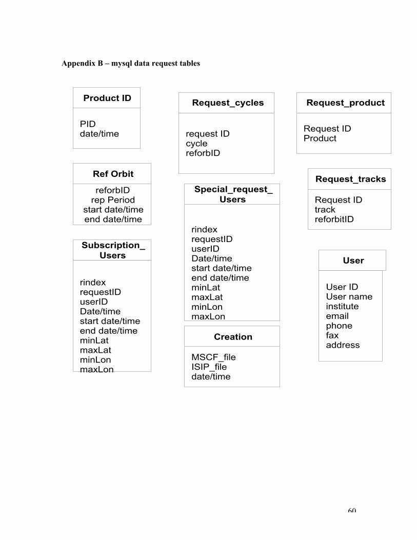
60

Appendix B – mysql data request tables

PID date/time

Product ID

Ref Orbit

reforbID rep Period

start date/time end date/time

Request ID Product

Request_product

request ID cycle reforbID

Request_cycles

Request ID track reforbitID

Request_tracks

rindex requestID userID Date/time start date/time end date/time minLat maxLat minLon maxLon

Special_request_Users

rindex requestID userID Date/time start date/time end date/time minLat maxLat minLon maxLon

Subscription_ Users

User ID User name institute email phone fax address

User

MSCF_file ISIP_file date/time

Creation