preliminary investigation of the environmental …
TRANSCRIPT

AD-AI726 688 PRELIMINARY INVESTIGATION OF THE ENVIRONMENTALSENSITV ITY OF ACOUSTIC SI.U) NAVAL POSTGRADUATE
US S D SCHOOL MONTEREY CA B B STAMEY DEC 82
NCAEhhmhh17/1hmu

Is.
IIIIN II~l ItI 8
MICROCOPY RESOLUTION TEST CHART
NATIONAL BUREAU OF SIANDADS 1963 A

NAVAL POSTGRADUATE SCHOOLMonterey, California
DTICQAPR t 2 W 3
THESISPRELIMINARY INVESTIGATION OF THE
ENVIRONMENTAL SENSITIVITY OF ACOUSTIC SIGNALTRANSMISSION IN THE WAVENUMBER DOMAIN WITH
RESPECT TO SOURCE DEPTH DETERMINATION
by
Billy Barton Stamey, Jr.
December 1982
Thesis Advisors: A. B. CoppensC. ". Dunlap
Approved for public release; distribution unlxinted
87' 83 04 11 123

Unclassified-"Cum" CI.ASS101CAYION OF VN4ls PA49 (Ubin 8th 8.k. ___________________
ftAD WNSTRUCTnflsREOMI DOCJUETATION PAGN sanvma C0"PL59TrS FORMV MW-R NU. @vt Accsion~~ 111111111"T-1 IGAl LOG WUmm
4. ?gL3 ~dbIE""le) Preliminary Investigation of the 14aer s Thesa iso oauEnvironmental Sensitivity of Acoustic Signal December 1982Transmission in the Wavenumber Domain with 6 apofoGa MOTwlesRespect to Source Depth Determination@UIGOG 3m uMR
7AuTwm(.~o a. CONTRACT OW G4&"T %,to-ginV.)
Billy Barton Stamey, Jr.
,UDV0OuhG 0010me2ATION MAUR AiND £000355 10 Assn.~ £~I~
Naval Postgraduate School24onterey .California 93940 N6846282WR200099
It. COwTOOLLWOG OFFICS WAWME AN. AODR6 12. 10POR? CATS
Naval Postgraduate School December 1982Monterey, California 93940 119mldaf
-U. IgIONITOENG16 A09MCV "AMEC GAOSUISMIE 00109MI he C==*e.5Otago 0fit. SICLIgTW CLASS. (09 thle rdbo"j
Commanding Officer UnclassifiedNaval Ocean Research and Development Activity IS AOSShF1CAON, 0000ma4GR01CCode 520 SCMEUL*1~ ~ ~ ~ ~ ~N 39529IU~O SAEU OS R
Approved for public release; distribution unlimited
17. ODISIUTlsam STAEICN? (01 00h0 0600 400 4108084 Is 8l00k 30. It difftea lf N06f)
1S. SuPOLSUIMARY 14079S
It. xIY 9000 (CiaflMS We 009111,0 @#do 1100400M Wi IEE~ffi SFAU NW)
he Wavenumber Technique (WT) is a relatively new method of underwatersound transmission analysis. One aspect, source depth determination, ispstudied to evaluate its validity and test environmental and acousticsensitivity. The horizontal wavenumber spectrum is analyzed to determinenull spacings in vavenumber apace, which indicates source depth by theLloyd's Mirror interference effect. Comparison of this theory with cases ofan isospeed sound profile, fully absorbing bottom, and flat totally-reflecting-
All0 73 vee O 01 Unclassifieri3/10 0162-814-6601)
SSCCUMTV CLASSFICAION OF Tme Plot ~De

Unclassified.vi nY ,, OTIH Y S 06Graen me so .
20.surface shows excellent agreement for several parametric variations. Caseswith realistic sound speed profiles and partially absorbing bottous generallyagree with theory, but a distinct bias is observed. Source depth determinationcurves, which relate scaled wavenumber spectral intensity null spacing to thesource depth, are presented for comparison with theory and sensitivityanalysis. An example is given for suggested application of source depthdetermination.
, D~.%Cod• Coe
i.o
DD FormI 1473 ti~ne- alif iadjak '3u' ~e~~~S PS SS ~

Approved for public release; distribution unlimited
Prelimina rTnvestiq ationof the Envi.ronmental1 Sensitivity of
Acousti Signal Transmissioni in the Wavenuaber Domainwith Respect to Source Depth Determination
by
Billy Barton Stamey Jr.Lieutenant ' Unite ite av46B.S., College of Charleston, 196
Sbitdin arti%.ffi1an oj the
MASTER OF SCIENCE IN METEOROLOGY AND 3CEANOGRAPHY
from the
NAVAL. POSTGRADUAWE SCHOOL
Author:_ _
Approved by:
3

ABSTRACT
The Wavenumber Technique (WT) is a relatively new method
of undervater sound transmission analysis. One aspect,
source depth determination, is studied to evaluate its
validity and test environmental and acoustic sensitivity.
The horizontal wavenueber spectrum is analyzed to determine
null spacings in wavenumber space, which indicates source
depth by the Lloyd's Mirror interference affect. Comparison
of this theory with cases of an isospeed sound profile,
fully absorbing bottom, and flat totally-reflecting surface
shows excellent agreement for several parametric variations.
cases with realistic sound speed profiles ind partially
absorbing bottoms generally agree with theory, but a dis-
tinct bias is observed. Source depth determination curves,
which relate the scaled wavenumber spectral intensity null
spacing to the source depth, are presented for comparison
with theory and sensitivity analysis. hn example is given
for suggested application of source depth determination.
f(

TABLE OF CONTENTS
I. INTRODUCTION ................ . 17
II. WAVENUMBER TECHNIQUE ............... 19
A. GENERAL DESCRIPTION .............. 19
B. PHYSICAL DESCRIPTION ... . . . .... . 23
C. WAVENUMBER TECHNIQUE APPLICATION ....... 28
D. TECHNIQUE LIMITATIONS ............. 30
III. PROPAGATION MODELS ...... . . . . . . . . 31
A. INTRODUCTION ....... . . .. 31
B. PARABOLIC ECUATION . 3
1. Introduction .. .. .. 33
2. Parabolic Approximation. ... 34
3. Brock Algorithm . . . . ........ 35
a. Description ........... . .. 35
b. Implementation .. . .. . 37
4. Subsequent Modifications .......... 41
a. Introduction . . . . . . . .-. . . . . 41
b. T .- 0 Modifiz-ations . . . . . . . . . 41
c. Stieglitz t Li Modifications 2.. . 42
5. SSFFT Evaluations .......... 45
6. Environmental Sensitivity of the PE .9. 49
C. FAST FIELD PROGRAM . .. ... . . . 52
1. General Description .... .. .... 52
5

2. Comparison of FFP and PE ......... 54
D. NORMAL MODE THEORY .............. 55
1. General Description .... . . . . . . 55
2. Comparison of NM and PE ..... 57
E. FINITE DIFFERENCE MEPHODS ...... 58
1. General Descriptions ... ... . 58
2. Comparison of FD and ODE with PE ..... 60
IV. ANALYSIS OF WT . .... .. .... .. ... . . 62
A. GENERAL DESCRIPTION. .............. 62
B. ISOSPEED CASES ... ... . . ... 87
1. Water Column Depth Variation .... . 87
2. Range Variation. ............. 89
3. Frequency Variatio n .... ... 89
4. Receiv'r Depth Viriation 96
5. Analysis of Isospeed Zases ........ 96
C. REALISTIC PROFILE CASES . .......... .100
1. Spatial Variaticn ........... 100
2. Temporal Variation . . . ........ 101
3. Range Variation .. ........... 105
4. Receiver Depth Variation ... . 105
D. COMPOSITE COMPARISON ............ 105
V. CONCLUSIONS . . . . ... .. . . . . . . . . . . 111
6

LIST OF REFERENCES .. .. ..................
INITIAL DISTRIBUTION LIST .. ............... 118
7

LIST OP ]!ABLES
TABLE 1. scenario Specifications .. .. 64
TABLE II. Location Information for Realistic Profiles 68
TABLE III. Compariscl Specifications . ... . 86

LIST OF FIGURES
Figure 1. Waveriumber Technique Flow Diagram. .... 21
Figure 2. Lloyd's Hirror Effect Geomqtry. ....... 26
Figure 3. WT Application for Source DepthDetermination. ............... 29
Figure 4. Space and time relationships of actualprofiles. .... .. . . . . . .67
Figure 5. Isos eed Profile Wa v erum ber Spectrum for SDo..f........................70
Figure 6. Isos eed Profile Wivenumber Soectrum fcr SDof 30 ft.71
Figure 7. Isos peed Profile Wdvenumber Spectrum for SDof 500 ft. .... .. . . . . . .72
Figure 8. Isos eed Profile Wavenumber Sp:ectrum for SDcf90ft. 73... . . .. . .
Figure 10. Isos eed Profile Wavenumber Spectrum for SDof 300 ft. . . . . . . .75
Figure 10. Realistic Profile Wavenumber Specrum fo:T SDof 2000 ft. . . . . 76
Figure 12. Realistic Profile Wavenumber Spsctrum for SDof 300 ft.....................77
Figure 13. Realistic ProfiAle W3vsnumber Spectrum for SDof 500 ft. .... .. . . . . . .78
Fi-gure 13l. Realistic Profile Wa venumbe r S pectrum f or SDof 800 ft. . . . . 78
Figure 15. Realistic Profile Wavenumber Spectrum for SDof 100 ft................ . .8
F igure 16. Realistic Profile waveniumber Spectrum for SD
of 3000 ft. . . . . 91
9

Figure 17. Isosped Profile Wavenuaber Spectrum for SDof 50 ft.. .............. 82
Figure 18. Example of Source Depth Determination Curve. 85
Figure 19. Isospeed Profile SD Determination Curve: ZVariation - 1. . 88
Figure 20. Isospeed Profile SD Determination Curve: ZVariation - 2. .. . . . . .. 90
Figure 21. Isospeed Profile SD Determination Curve: ZVariation - 3. . . .... ......... 91
Figure 22. Isospeed Profile SD De-termination Curve: ZVariation - 4. . . .............. . 92
Figure 23. Isospeed Profile SD Detrmination Curve: RVariation - I............ ... . 93
Figure 24. Isospeed Profile SD Determination Curve: RVariation - 2. . ............... 94
Figure 25. Isospeed Profile SD Determination Curve: RVar-_ation - 3. . ............... 95
Figure 26. Isospeed Profile SD Determination Curve: FVariation -1. . . .............. 97
Figure 27. Isospeed Profile SD Determination Curve: FVariation -2. . ................ 98
Figure 28. Isospeed Profile SD Detarmination Curv-: RDVariation. .................. 99
Figure 29. S atial Variation (&,B): SD Dgt rmination andAXBT Curves . ............... 102
Figure 30. Spatial Variation (C,D): SD Detsrmination andAXBT Curves ................ 103
Figure 31. Temporal Variation (A,C) : SD D-ermninationand AXBT Curves. . ............. 104
Figure 32. Tem poral Variation (B,D): SD Determination
and AXBT Curves .............. 107
Figure 33. Range (R) Variation for Profile A ..... 108
Fiqure 34. Receiver Depth (RD) Variation fcr Profile. A. 109
10

Fi-gure 35. Compositip Comparison for Isospeed andRealisti Cases. 110

TABLE OF SYMBOLS
s attenuation coefficient
B m scaled wavenumber
a envelope function
X a reference wavelength0
angular frequency
p a density
e = beau elevation (depression) angle
s = central-difference operator
= 3.141593
7 = Laplacian operator
a = partial derivative operator
= summation operator
= integral operator
= square root operator
<< - much less than
C = sound speed
C = minimum sound speeda
C normal mode phase speed
= Lloyd's Mirror pressure field in ra.age space
f - frequency
F = Lloyd's Mirror pressure field 'n wavenumber space
G - Green's function
12
i

H = Hankel function0
I spectral intensity
lIMT a imaginary pressure transform
JO= zero order Bessel function
K a total wavenumber
k r= horizontal wavenumber component
kr 0 = initial spectrum wavenumber
kZ= vertical wavenumber compoaent
Ak a wavenumber increment
K = maximum wavenumber
M = complex modified index of refractioa
n - index of refraction
= modi:'fied index of refracti-A.on
nb= water/bottom interface index of ref.-action
NT = spectrum index
P = acoustic pressure
R = range
AR = range increment
Re, = :ea. pressure transform
'a = wave speed
Z - water column dep~th
Z a modified water column depth
A7 = depth lncrament
13

Z R a receiver depth
zS= source depth
Z a maximum depth in transformmax

&CKNOWLED3 ElENT
Dr. A. B. Coppens showed great kindness by accepting
supervision of this research when time was short. Vis con-
cern, understanding and direzticn led to an investigation
which is believed to te successful. He can both profess and
teach. This research and my personal development benefited
greatly from this unique ability.
LCDR C. R. Dunlap, USN (Ret) was very supportive and
encouraging during my entire thesis rssearch effort. I
appreciate his assistance with this projezt and his excel-
lent work with the NPS Environmental Acoustics Research
Group (EARG).
Richard Lauer of the Naval Ocean Research and Develop-
ment Activity (NORDA) developed the WT co-cept which was the
basis for this research. My thinks to him for allowing this
investigatio of his idea and his assistance during the
study. Tom Lawrence of Ocean Data Systems, Inc. (DDSI) at
NORDA was my principal contact during thi-- research and fu:-
nished its fcundation. I appreciate the try hcurs :f tele-
phone conversation and his liaison at NORDA. Richard Evans,
also of ODSI and NORDA, provided great as-istance in devel-
:ping the computer software and my understanding of the mod-
els.
15

I also thank C.N. Spofford and Eleanoc Holmes of Science
applications, Inc., John Locklin and Gil Jacobs of ODSI, and
Jim Davis of Planning Systems, rnc. for their assistance.
The personnel of the NPS Dudley Knot Library Research
Reports Division and the 1.R. Church Computer Center were
also very helpful during this research.
My thanks also to my family for thseir patieace and
understanding, and to my colleagues in the BA~RG for their
advice and assistlance.
16

The Wavenumber Technique (WT) is a new method for the
solution of several problems related to the analysis of
underwater sound transmission (Lauer,1979). Its basis is the
analysis of acoustic propagation in the wavenumber domain,
which has been described by DiNapoli (1971) and was an
intermediate step in the computation of transmission loss
versus range in the Fast Field Prograz (FFP) . DiNaoo!i
(1977) later used the wavenumber domain to study the impe-
dance of the ocean-bottom Interface. Lauer (1979) first
introduced the WT and its applications to passive localiza-
tion and tracking and multipath decomposition. He developed
a range prediction curve based upon peak wavenumbers in the
transform spectrum fcr successive range increments from an
entire pressure range field.
These investigat ions presented highly beneficial and
promising results from the wavenumber depic':ion, which indi-
cates that additional research is appropriate. One particu-
lar aspect of the WT - determination of source depth - will
be investigated here in order to evaluate its validity in
comparison with the Lloyd's Mirror effect. Its relation-
ships to oceanic and acousti= variations will also be
examined.
17

The wavenumber technique as first described by Lauer
(1979) was based upon input from the FFP, but it has been
adapted for use with the Parabolic Equation (PE) method of
propagation loss determination. The PE-based WT is currently
being investigated by Lauer and others at the Naval Ocean
Research and Development Activity (NORDA) and was the model
used in this research at the Naval Postgraduate School
(YPS). Descriptions of the PE and WT will be presented to
display their sensitivities to variations of several model
parameters. Also, exrected relationships of the WT to other
current propagation prediction models will be discussed to
consider how results might vary based upon different inputs.
Particular attenton will be given to algor-ithm differences,
degrees of approximation, and treatment of the ocean bottom.
The PE-based WT will then be exercised for several
parameter variations to evaluate qualitatively the consis-
tency of the technique. This study will also demonstrate
the response of the PE-based WT to geomet-ic and actual
oceanic conditicns. Prediction curves fo: source lep-.h
determinaticn based upon these variations will be presented
and discussed.
j1

TF
A. GENERAL DESCRIPTICN
The UT is a natural alternative for signal depiction
because it provides information on the directions of energy
arrivals. It allows reasonably direct physical interpreta-
tion of ocean acoustic processes and their relationships to
environmental conditions (Lauer, 1979). Lauer further states
that the wavenumber spectrum plot is clearer and more
informative than typical curves of propagation loss versus
range. The wavenumber K relates the angular frequency and
'he sound speed by
K = w = 27f
C C
and it has horizontal and vertical components
K = k r+ k
The reference wavenuiber is determined by the sound speed
mi ni mum
K0-
C0

The WT will first be described without reference to any
particular propagation model to present the general nature
of the algorithm. Fig. 1 is the flow liagram for the WT.
The left and right sides of this flow diagram correspond to
the intensity and wavenumber axes, respectively, of the
spectrum plot that will result from the WT. This figure and
the following discussion were developed from Lauer (1979 and
1982a) and augmented by several telephone conversations with
R. Lauer, T. Lawrence, and R. Evans of NORDA between July
and December, 1982.
The WT calculates spectral intensity from the real and
imaginary parts of the acoustic pressure
p = (R,Z) e
The complex psi versus range field at a specified depth is
the propagation model product which determines the pressure.
The complex pressure field can be modifi-a-A for effects such
as attenuation, depending upon whether i.Ialized or realis-
tic conditions are being investigated. A Fast Fourier
Transform (FFT) is then applied to yield transformed complex
pressure. The spectral intensity is 1e9ermined at each
23

WAVOSAOM TECHNIWE FLOW DIAGRAM
PROPMODEL
SELECTEDaftsm VARIABLES
REAL& 114AG
MODIFY ALPRESSURE 1 S"VIEFIELD I NUMBER I
FAST WAVEF OUR I ER NUMBER
TRANSFORM IINCREMENT I
TRANSFORMCOMPLEXPRESSURE
I ISPECTRAL ETA
INTENSITY SCALED!AXI _j A
WAVENUMBER
SPECTRUM
MEASUIREMULL EPT14
(]SA k>==* I SIETOEIRMCURVE
Figure 1 4avenumber Technique Flow D-L-agram.
21

wavenumber increment from the transformed complex pressure
field by
I ReT 2 + ImT 2
s T T
This intensity field is scaled arbitrarily for satisfactory
display of the relative maxima and minima to define the
intensity nulls.
Additional output parameters from the PE which are
required for the WT include the range step, the number of
range points, frequency, minimum sound speed and field
depth. These are the selected variables noted in figure 1.
The range step is selected to provide sufficient resolution
to determine the wavenumber null spacing on the spectrum
plots. The initial radial component of the wavenumber for
the spectrum is calculated from DiNapoli (1971) by
k :K -27rrao o -
AR
where
: =k +k
o ro ZO
22

As will be seen in section I1-B, if a "scaled" wavenum-
ber beta is used for the horizontal axis, analysis is sim-
plified since the nulls in the spectra should be more evenly
spaced (Lauer,1979). The physical meaning of beta will be
described in the next section. The resulting scaled wave-
number spectra are then plotted. The wavenumber null spacing
for each incremental source depth is determined from each
scaled spectrum. The source depth dete.mination curve is
generated by plotting these null spacings as a function of
source depth, as suggested by Lauer (1979). The null spac-
ing cf an analyzed received signal could be compared with
this determination curve to infer the source depth of the
signal. This application will be discussed later. The
source depth determination curve will be specific for the
acoustic and oceanic descriptions of the medium.
B. PHYSICAL DESCRIPTION
The preceding description was intended to provide the
overall concept of the WT whereas wha- follows will explain
the physical basis for the technique. The underlying princi-
ple of the WT as described by Lauer (1982a) is the Lloyd's
Mirror effect, which gives the acoustic field by
p E(R) e iwt
23

where
E(R) exp {iK /R2 + (ZR - )2} - exp {iK /R2 + (Z R + ZS) 2}
/R2 + (ZR _ ZS)2 R2 + (ZR + ZS)2
for a point source in a semi-infinite zedium of constant
sound speed with a pressure release surfice. This is the
Lloyd's Mirror field in range space, whereas the Lloyd's
Mirror field in waven.umber space, applicable to this
research, is given by Lauer (1982) as
F(K) = sin( .ZS ) exp(iaz R )
where beta is defined by
= (K 2 _ k 2)
and E(R) and F(K) are related by the Bessel transform par
E(R) = f'2 F(K) J (KR) K dK0 0
and
F(K) = I ;"E(R) J (KR) R dR
214

For this research the Bessel fujnction was approximated as a
trigonometric function so that the FFT could be uti,.lized.
This is considered acceptable since tha source and receiver
are greatly separated, according to Lauer (1982b). Inspec-
tion of r(K) reveals that the nulls of the spectrum will be
equally spaced at intervals of
z s
This equal spacing in beta is the key element of the appli-
cation of the WT to source depth determination (Lauer,1979).
Only the direct and surface-reflectal waves will inter-
act at a receiver location in a simple illuastration of the
Lloyd's Mirror effect with a smooth surfa-ce. This interac-
tior. will be destructive or constructive, as a result of
their relative phases (Kinsler -at al 1982) and will produce
n-ulls or peaks, respectively, in the wavenumber spectrum.
Fig. 2 depicts the Lloyd's Mirz:)r effect geometry which will
be used to study test case outputs for null spacing and sub-
sequent source depth determination. Zhe surface-reflected
(SRI wave travel distance will increass at a -faster =ate
than the direct (D) wave distance as the source Is moved
25

SHALLOW SOURCE
Surface
SAC ACV
Bottom
DEEP SOURCE
________Surf ace
I-
ACV
d
SRC
Bottom
Figure 2. Llcyd's Mi rror Effect Geometry.
26

deeper in the water cclumn (1) while the receiver depth (h)
is stationary. This leads to different arrival patt-rns and
nulls at more wavenumbers. 7hus the general pattern of
decreased spacing in beta with inzreasing source lepth is
observed.
Eottom interacting waves will be neglected for idealized
cases. This will be accomplished by the use of a fully
absorbing bcttoa. These waves will be important, however,
in shallow water or at greater ranges. & fsw test cases will
have realistic bottoms. Various propagation models handle
the bottom in different ways, so the inzlusion of a bottcm
will be discussed later. Cas-s in shal!ow water (less than
5000 feet) or at extended ranges (great-r than 100 miles)
will not be considered here.
Lauer (1979) observed that the wavenuabSr spec-rum shcws
a series of modulating envelopes which enclose spikes :hat
are the eigenvalues associated with th% normal modes. Com-
parison of the wavenumber spectrum with typical transmission
.oss curves reveals that the wavenumber Aepiction 4s more
coherently structured. This leads t: a better physical
understanding of signal transmission because of th _ rzla-
tionship between horizontal wavenumber aad :ay -heory. He
gives this ask cose 2'f Cosa
27

The horizontal wavenumber decreases as theta increases. Thus
the wavenumber axis of the spectrum plot will include wave-
numbers associated with smaller elevation (or depression)
angles in increasing crder of wavenumber (Lauer,1979). It
is then expected, for the case of a neglected bottom, that
spectrum amplitude peaks could be observed that would corre-
spond to the direct and surface reflected waves.
C. WAVENUMBER TECHNIQUE APPLICATION
Lauer (1979) reco-mmends a receiver that is a single
omnidirectional hydrophone and a source-g-nerated continuous
wave (CV) received signal for source depth determination.
He further states that in actual use the single hydrophone
could be replaced by an array to improve the sional-ro-noise
ratio and to obtain bearing and bearing rate 4nformation.
An example of a possible application of the WT, scurce
depth determination, is presented in Fig. 3. A propagation
model could be run for a series of incramen+al source depths
to yield the null spacing relationship, as was shown in Fin.
1. That curve would be specific to the properties of the
ocean and values for parameters such as frequency and
receiver depth. A received signal as shown on the right side
of Fig. 3 could then be analyzed. Its null spacing could be
28

VT APPLICATION: SOIRCE DEPTH KCTER4MTION
VARYINMG1PROP MODE
COMPLEXRECEIVEDPRESSURE SIGNAL
F0IELD
FAST FASTFOURIER FOUR IER
TRANSFORM ITRANSFORM
WAVE WAVENUMBER NUMBER
SPECTRUM SPECTRUM
MODEL S IGNALNULL NULL
SPACING SPACING
Figure 3. VT Application for Source Depth Determination.
29

comparel to the model-producel curve to infer the depth of
the source.
D. TECHNIQUE LIMITATIONS
The success of the WT is related directly to the accu-
racy of the predicted pressure field produced by the propa-
gation model. There are several possible differences
between propagation models whizh might affect the pressure
field. Some of the more significant include approximations
of the wave equation, bottom effects, initial source func-
tions and input limitations. These will be compared for sev-
era! models to determine relevant restrictions. The pressura
field will also respond to chaages in the ocean. A series
of different scenarios will be run to provide an initial
es-.imate of the sensitivities to some of these factors.
Any additional limitations will be related to computer
processing time and storage requirements. These factors will
not he addressed directly in this resear:h because the pro-
cessing following the propagation model is minimal. There is
also no requiremqnt tc store the complex pressure fields or
their transforms once the null spacing has been determined.
Thus the WT computer utilization is directly proportional to
the time and storage required for the propagation models.
30
i

III. PROPAGJJI =241Da
A. INTRODUCTION
Modeling the propagation of sound in the ocean is com-
plicated by the variability of the ocean, the great range of
frequencies of interest, and the many applications of sound
propagation (DiNapoli and Deavenport,19791. It is not sur-
prising that no single model is presently capable of
addressing all of these variations; there are many semi-re-
strictive methods. In general all models consider the sound
speed to be a function of the spatial coordinates and inde-
pendent of time (DiNapoli and Deavenport, 1979). Only the
frequency, water column geometry and ozeanic description
will affect propagaticn.
All models, regardless of application, can be divided
into two classes: range independent or range dependent.
Range independent models assume that the ocean is cylindri-
cally symmetrical, te speed of sound is a function only of
depth and all boundaries are planar pe.pendicular to the
depth axis (Di.1apoli and Deavenport, 1979). Range dependent
models can provide better approximations of real conditions
31
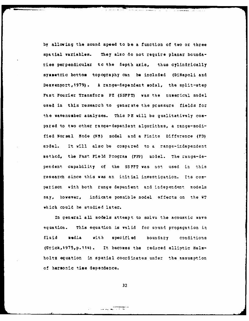
by allowing the sound speed to be a function of two or three
spatial variables. They also do not require planar bounda-
ries perpendicular tc the depth axis, thus cylindrically
symmetric bottom topography can be included (D±Napoli and
Deavenport,1979). A range-dependent model, the split-step
Fast Fourier Transform PE (SSFFT) was the numerical model
used in this research to generate the pressure fields for
the wavenumber analyses. This PE will be jualitatively com-
pared to two other range-dependent algorithms, a range-modi-
fied Normal Mode (NM) model and a Finite Difference (FD)
model. it will alsc be compared to a range-independent
methcd, the Fast Field Program (FFP) model. The range-de-
pendent capability of the SSFFT was not used in this
research since this was an izitial investigation. rts com-
parison with both range dependent and independent models
may, however, indicate possible model effects on the WT
which could be studied later.
In general all models attempt to solve the acoustic wave
equation. This equation is valid for s:und propagation in
fluid media wit h specifi ed boundary conditions
(Urick,1975,p.114). It becomes the rediced elliptic Helm-
holtz equation in spatial coordinates under the assumption
of harmonic time dependence.
32

B. PARBOLIC EQUATION
1 ;A tr 01I11-
The PE algorithm used i this research was laveloped
by Brock (1978). The basic feature f this PE is the
replacement of the reduced elliptic Helmholtz equation by a
parabolic partial differential equation that utilizeas the
Tappert-Hardir split-step Fourier algorithm (SSFFT) for the
numerical integration (Brock,1978). The original computer
code as described by Brock has been modified to incorporate
-he source and a'tenuation descriptions ot Tatro (1977) and
to include an ocean bottom by Stiglitz 94 al (1979w. This
is the version of the PE that is currently available at NPS
ard was the code (PERODEL) usel for this r-.earch. (it must
be emphasized that some difficulty was enzountered in trying
to ascertain the correct desaription :f the NPS version
because of inadequate and erroneous comm=nt card documenta-
tion in the source code and incomplete manuscript descrip-
tions.)
This section will disCuss the SSFFT, the original
Brock algorithm, modifications to that cola, and subsequent
4valuations of the SSFFT. Particular it-ention will be
given to those aspects which are expected to affect the WT.
31

2. RaLk2 i IR-2 1 21 12
The parabolic approximation to the wave equation was
first introduced by Leontovich and Fock (1946) as a solution
for the propagation of electromagnetic waves along the sur-
face of the earth. Its first introduction to underwater
acoustics was by Hardin and Tappert (1973) who used the
split-step technique in conjunction with the FFT to solve
this particular apprcximation to the wave equation. The
result was the SSFFT. Tappert (1977) related the use of the
parabolic approximation to sound channel propagation in a
waveguide that is thin vertically and elongated horizontally
to the range of the first convergence zone or farther.
Long-range propagation, with which the SSFFT is
basically concerned, will usually be for low frequencies
because volume absorption increases strongly with frequency
(Tappert,1977). The maximum elevation (and depression)
angles of propagation for long range transmission must be
small to satisfy the FE (Tappert, 1977). The derivation of
the SSFFT will be discussed later in a simplified version as
presented by Brock (1978).
It appears that the SSFFT is intended for use ir
situations where bottom interaction and surface scattering
34

would be negligible. Thus the use of the SSFFT to examine
the Lloyd's Mirror effect in the real world may be inappro-
priate if the ocean surface is sufficiently rough; addi-
tional errors may occur in situations where bottom effects
are sign ificant.
3. B lo hm
a. Description
The SSFFT is valil for acoustic pressure in a
medium of constant density with a monofrequency source and
cylindrical symmetry about the lepth axis (Brock,1978). The
acoustic pressure can be written as
p(R,Z) = P(R,Z) H I(K R)
where the zero-order Hankel furction of the first kind
relates the acoustic pressur_ to an outward propagating
cylindrical wave envelope function (Brock, 1978). This is
valid because of the assumption that at low frequencies all
significant energy will propagate approximately horizontally
away from the source (Tappert,1977). The asymptotic form of
the Hankel function is
H I(K R) -21nK R} expti(K R - n, K R >> 10 0 0 0 0
35
HII i

if the receiver is many wavelengths from the source. This
leads to (Brock,1978)
*RR + 2 iKo*R + ZZ + K02 {n2(RZ) - i}j - 0
The additional assumption of neglecting the far field
effects,
I RRI '< j2iK o Rj
is the "parabolic' approximation for r~dial transmission
(Brock,1978). The result is the Leontovich-Fock (1946) PE
R i(A+B)
where
A -2
2K az20
and
B = Ko 2 (n 2 - 1)
36

which is the form used by Brock (1978).
b. Implementation
Brock (1978) used the SSFFr to solve the PE
because it has several significant advantages which outweigh
its disadvantages. Advantages include exponential accuracy
in depth, second-order accuracy in range, energy conserva-
tion, unconditional stability and computational efficiency.
Disadvantages are a uniform mesh and periodic boundary con-
ditions to satisfy the FFT, and filtering of tho sound speed
profile by smoothing discontinuities to avoid spurious high
angular-frequency components (Brock,1978). Additionally the
algorithm assumes a flat pressure-r.3lease surface, a vanish-
ing field at the maximum depth and a pseuJ3-radiation condi-
tion at the water-bottom interface by smoothly att-nuating
the field (Brock,1978).
A numerical algorithm of
' R = i(A+B) I
(R+aR,Z) = ei IR(B+A) (RZ)
leads to
p(R+AR,Z) = e A R B FFT- FFT ((R,Z)) }
3-

or
4(R+AR,Z) = e o FFT-l{e 0FFT(*(R,Z))}
to facilitate the computations since a spatial FFT and its
inverse are required to transform between dpth and wavenum-
bet (Brock, 1978) . This procadure is implemented by two
alternating steps, the first of which considers propagation
in a homogeneous medium to account for Eiffraction and the
second to account for refraotior (Bro=k,1978). In his
development Brock gives an ilternate zalculation of the
envelope function stemming from
'(R+AR,Z) = e iRA/2 e iA R B eiARA/2 (RZ)
This differs slightly from the previous expression zontain-
ing the FFT and inverse FFT. Thus it is -ot currsntly known
which relationship is used by Brock; this could be resolv=d
later by a detailed examination of the :zompuer code. In
any event as McDaniel (1975a) has shown, either approach
would be of sufficient accuracy with appropriate selsction
of AR and AZ.
33

The SSFFT appears to be juite satisfactory
numerically, but it has to simplify the actual oceanic vari-
ability to allow realistic cclputation. It apparently will
handle source and receiver depths and horizontal separation
distances well as noted by its degrees of accuracy in depth
and range. The smoothing of the sound soeed gradients and
bottom effects will have to be considered.
The intent of this descriptioa has been to pro-
vide a base from which comparisons can De made with other
numerical solutions and modifications t this algorithm.
The effect of the source model on the WI can be evaluated by
these comparisons. The primary elements of the WT are the
real and imaqinary parts of the complex pressure amplituds.
Thus the algcrithmic differences with =espect to computation
of the pressure field will be the primary basis for the com-
parison of effects on the WT.
McDaniel (1975a) compared th_ basic Tappert and
Hardin SSFFT, which is used by Brocc, to aormal mods theory.
She found that errors arise in phase and group speeds,
although one mode can be propagated with the correct ampli-
tude and group and phase speeds. McDanie! describes three
sources of error: (1) approximating the wave equation by the
39

SSPFT as noteId above, (2) limiting the range s-teps and per-
Missible sound speed gradients, and (3) t-run~cating the fiell
at a finite depth. The result Df the SSFT will be a shi;ft
in. the model interference at long ranges if many modes are
propagating (fcDaniel,1975a). The error due to range step
limi-tations is third order ;-a the range step increment
(McDariel, 1975a) , thus a small range step is rsquired --o
mi6nimi-z this error. The third error Is related to inClusion
of a highly absorbing bottom which causes preferential
attenuation cf higher-order modes; the domi-nant contribution
w ill thus result from the lower modes (McDanial,1975a).
Brock et al (1977) have described a procedure
to i-mprove this condition. It maps the index of refraction
and depth such that the phase speeds and turnirg points of
the normal modes are preservei1. This involves construction
of a "pseudoproblem" such that the parabolic phase speeds
w ill be equal to the ellipticz phase speeds of the corre-
sponding modes in the original problem (Brock ; a! 1977).
This Is gi1ven as
40

It is found to greatly improve the SSFPT agreement with the
elliptic solution. This correz-tion technique has one basic
constraint, which is that isospeed regions are not allowed
in the sound speed profile because of poor eigenfunction
mapping (Brock pt q,1977).
4. §ubsect.2.12 Ag.Licati2j
a. Introduction
There have been two significant modifications
since the original algorithm was published by Brock (1978).
These are source function and volume attenuation altc-rations
(Tatro,1977) and the incorporation of a bottcm and variable
range step (Stieglitz et al ,1979) . The Tatro modifi41cation
was developed in 1977 but was added to the Brock algorithm
after 1978. Discussion of thase two aspects will complete
the description of the PE algorithm Installed at 11PS and
utilized i;n this study.
b. Tatro Modifications
The Gaussian source originally utilized by Brock
(1978) was considered to be inefficient in trms of program
size lijmitation and an upper frequency limit which is :ela-
ti-vely low (Tatro,1977). A new source fanction was devel-
oped. This was i.ntended to solva! the problem of large
41

vertical wavenumbers from a Gaussian source that were previ-
ously eliminated with range (ratro,19771 and lei to an
incorrect depiction of the fiell.
This source is basically a low pass filter in
4he vertical wavenumter domain which is centered at the
source depth (Tatro, 1977) . The initial vertical wavenumber
field will thus be a constant up to a prescribed value and
zero for higher wavenumbers. The use of the filter is
claimed to yield improvement over the Gaussian source by
minimizirg the aliasing which might occur upon transforming
to the depth domain (Tatro,1977). rhe beaefits derived from
the use of this new scurce are reduced computation time and
storage and the availability of higher frequencies
(Tatro,1 977).
He also modified the Brock algorithm by intro-
ducing volume absorption as calculated from the qquation of
Thorp (1967) . The decision zan be made whether or not to
include volume absorption.
C. Stieglitz get al Modifications
Brock (1978) had considered the PE most useful
for lcnq range propagation a: low frequencies and small
grazing angles. The bottom was sodeled as fully absorbing sc
42

that the field would vanish at the maximum depth of the
transform. This depth was obtained by extending the water
column depth by one-fourth to obtain the transform depth.
The index of refracticn in this region was
-2 + iae (zz )/b} 2
nb ae max
where a and b are empirical constants. The energy in the
bottom was attenuated such that any additional modes which
resulted from transform truncation were minimized. This
empirical expression was selected to coincide with a compa-
rable normal mode solution. This rather crude model of the
bottom appeared to be acceptable for sitiations wherein the
bottca had a relatively small affect.
Stieglitz et al (1979) considered it nezessary
o attempt to develop a more realistic ocean bottom since
acoustic propagation was being utilized in more varied and
extreme situations where bottou interaction was important.
They developed two additional options for handling the bot-
tom: (1) a partially absorbing bottom with specification of
reflective loss versus grazing angle of :he equivalent ray
and (2) the direct insertion of sediment sound speed and
43

attenuation profiles. The algorithm derives the sediment
profiles from the grazing angle loss values in the first
opticn. The supplied profilss are used directly in the sec-
ond option (St ieglitz _q Al , 197 9) . A new complex modified
index of refraction
M(R,Z) ={n 2 (R,Z) - 1} + i2b(Z)/K0
is computed i*f the bottom atteriatian is to be calculated.
One additional chaage, the zalculation of the
range step, has also been added by Stieglitz t al (1979).
1I6 consists of an initial search of the vertical wavenumber
domain for the maximum prsssurs component. This is then fol-
lowed by a search for the first component whi-ch is 50 dB
below the maximum component. The wvsvnumber of :hi4S
cornpcnen t
k K 50n
is stated to :equire a range step of
AR X 0/(1 - Cose 50
414

where
X 21/K0 0
The range step was fixed in the currant research for the
benefit of the spatial transform in the WT, thus the above
description was not utilized. It has been included to com-
plete the description of the -omputer cola which apparently
comprises the NPS model, PEMODEL.
5. EvlUjoU
The SSFFT has been investigated oa several occasions
to examine specific items which might be modified to yield
better agreement with actual propagatioa. Most of these
studies deal with the algorith2ic description by Tappert and
Hardin (1973). Examination of these stulies will note fur-
ther possible limitations on a-curacy in the SSFFT which can
be extended to the WT.
Fitzgerald (1975) examined the accuracy of :he SSFFT
as a functior of range and frequency. I-: was shown that the
SSFFT demonstrated greater accuracy at longer ranges, the
lower the frequency. The SSFFT was considered a gcod
approximation in the examples given for 100 HZ and 10 HZ :o
45

about 111 and 15000 kin, respectively (Fitzgerald, 1975).
The current study vil examine transmission at 50 and 100 HZ
at ranges to 100 nautical miles. These ranges will exceed
the limits of Fitzgerald in some cases.
McDaniel (1975b) investigated splitting the total
field into transmitted and reflacted fields in deriving the
SSFFT. It was necessary to neglect the reflected field for
the matrix associated with the Tappert-Hardin SSFFT, since
the two fields did not decouple where the wavenumber was
independent of range (McDaniel, 1975bi. Thus an exact
expression could not be determined for the transmitted field
without the reflected field. (The reflected field is neg-
lected in the current researt-h since it uses the SSFFT.)
This will lead to phase speed and group speed errors as
McDaniel (1975a) pointed out earlier, as discussed in Sec-
tion III-B-4. These errors were minimized by Brock et al
(1977) by a mapping technique for both the index of refrac-
tion and the depth. Even so, the implication of -his pcssi-
ble error cn the WT is that the interfers.nce -- :erns may
not be exact, which will lead to inexact 3r biased wavenum-
ber nulls. McDaniel (1975bi proposed another matrix which
achieved the desired decoupling and thus allowed expressions
46

for the transmitted and reflected fields. This alternative
was not investigated in this initial research. It may be a
way to resolve non-exact results and could be studied later
to isolate quantitatively the biases related to various
input parameters for the WT.
Palmer (1976) related possible inaccuracies in the
SSFFT to approximations involving relatively small terms in
the exponential approximations for the operators A and B and
also to the use of a single reference wavenumber. These
apprcximations will nct be investigated specifically in this
research but they may be related to potential disagreement
between the SSFFT and the theoretical Lloyl's Mlirror effect.
The association of errors due to a singl- wavenumber can be
recognized from the wavenumber spectra, which will be pri-
sented later in section IV-A. They will show not only an
energy concentration at the ref.rence wavenumber but signif-
icant energy distributed, as well, over a range of values.
Palmer (1976) emphasized that the physical properties of the
ocean must be considered before terms can be neqlected, such
as the spreading of energy over several wavenumbers.
DeSanto (1977) studied the relationship between the
acoustic pressure and the envelope function (called velocity
47

potential by DeSanto), which is directly relevant to the
current research where pressure is calculated from the mod-
eled envelope function. DeSanto arrives it
*(R,Z) =A R 1-af-P(t,Z) Q(R,t,Z) exp CUK /Zt)(R 2+t2) ta-3 / dt0 0 0
where Q satisfies
RR+ 2((l-a)/R +(iKOR)/t}QR + Q 7+ 2iK Qt + 2Qza L{(p(t,Z))
K 02{K 2(t,5Z) - K 2 (R,Z)IQ
and
K2 (,)=K(R,Z) - K~)-
The PE for the envelcpe function is obtained if this f~unc-
tion is evaluated by stationary phase; thas, It appears that
a more accurate result could be obtained by better eva.A.ua-
't.on of the integral. DeSanto et 1 (1978) developed a cor-
rection for the SSFT, known as the Corrected Paraboi-c
'48

Approximation (CPA), that handled phase inaccuracies better
than the SSFFT. Further study might address the response of
the UT to the CPA with respect to improved phase accuracy as
a function of range.
6 Zairn a jinsitilit.1 of thg E
This final section in the analysis of the PE will
consider the expected environmental sensitivity of the PE,
and, by extension, the WT. The important relationship of the
PE to the UT is the input of the complex pressure amplitude
and ultimately the resultant wavenumber distribution. As
discussed earlier in Section Il-B, the wavenumber could be
associated to the source angle and, by extension, to the ray
type or family (Lauer, 1979). Consequently, oceanic parame-
ters which modify the transmission of certain rays can be
related to the resulting wavenumber distribution.
The sound spead profile will favor certain ray paths
at different depths in the water column. There should be a
corresponding shift in ray paths and hence wavenumbers as
the source and receiver depth geometry is changed. The
direct and surface-r eflected rays will travel at different
speeds depending upon the gradients along the profile and
thus lead to different spatial interfereace patterns. This
'49

can leal to wavenumber shifts and changes in the null spac-
ing. Profiles used in the current study will include real
examples and isospeed cases.
Another important aspect is the transmission geom-
etry. Generally the model will be run at considerable range
and in relatively deep water, which will be consistent with
the applicability of the PE. A series of source depths with
a single fixed receiver depth will be run to generate the
wavenumber null spacing values that will formulate a deter-
mination curve for each case of geometri:al variation. The
distribution of these resulting curves can be examined to
evaluate the effects cf transmission geometry on the WT.
Two frequencies will be ixamined ir. a similar man-
ner, This would be one of the most important parameters to
investigate in future studies since it would have a dir-ct
bearing on operational applications. It is expected that
there will be differences in the resultiag wavenumber spec-
tra depending on the input frequency. The relationship
between frequency and transmission geometry will also be
studied since these are the easiest paraeters to vary dur-
ing an experiment and will lead to the most complete analy-
sis of model variability.
m50

The surface will be assumed to be planar and pres-
sure-release so that there will be complete specular reflec-
tion. The minimum source depth used will be that at which a
definable interference pattern -an be observed for the spec-
ified frequency. The slope approaches zero near the surface
on the source depth determination curves. This result may
indicate that the WT in its current form is probably not
applicable for sufficiently shallow sources.
The final important area of variability will be the
bottom boundary conditions. There are several options now
available in the PEMODEL. The fully absorbing and partially
absorbing bottoms will be considered. A fully absorbing
bottcm will be used in most cases to simplify the interfer-
ence pattern by elimitating any rays which interact with the
bottom. Thus the basic interference pattern may be evalu-
ated. Varicus bottoms can then be tested to study the
effect of the bottom on the dT. Differing bottom icss
curves will be comparsd in a few cases to lemonstrate quali-
tatively that the bottom does have an sff-ct. The third bet-
'om option of a realistic sediment sound speed could also be
investigated once the general effect of the bottom has been
determied. it would not offer any additional significant
51

results at this point beyond those realized from the fully-
and partially- absorbing bottoms.
All input parameters are related and thus the exami-
nation of any one particular factor must be considered with
respect to the full range of variation of the other factors.
The number of combinations of parameters would be very large
for a model such as the PEMODEL. Thus this research can
only begin to explore general relationships. Additional
research is necessary to delineate specific parameter
impacts on the WT.
C. PAST FIELD PROGRA
1. General Descri pion
The Fast Field Program (FFP) was selected as the
first model to compare to the PEMODEL siaze it was the cri-
gin of the WT and the initial testing :f the WT by Lauer
(1979) was performed with the FFP. The description of the
FFP which follows is summarized from Dilapoli (1971).
The basic result of the FFP is direct numerical
inteqration by the application of the FFT to field theory to
compute propagation predictions _n a minimum computation
time. The pressure can be represented in the form
p(R,Z) y-_07f0 G(Z R ;K) Ho1 (KR) K dK
52

where G, the Green's function, must satisfy
d 2G + {K 2 (Z)-k 2 )G = -&(Z-Z )
dz2
and the associated boundary conditions. The field equation
can then be written as
iKR Ri m R AKp(ZR m) V- AK(2/ii) e o Rm /Rm E e o
where
eimR AKEm = G(Z,ZS;K m ) K m e A
In this form, p can be obtained through use of the FFT at
each range increment. Given p is a function of range, the WT
could be applied as usual. D iNapoli compared an example
from the FFP with the normal aode progran of Bartberger and
Ackler (1973) and found excellent agrsement between the
locations of the peaks and the real parts of --he eigenval-
ues. The only significant 3ifference is that the FFP
includes more higher order moles but doss not ,nclde the
53

first four modes. DiNapoli states that the FFP offers a
significant reduction in computation time yet still provides
reasonable results as compared to normal mode theory. This
is accomplisbAd by expressing the sound velocity profile as
one or more exponential functions of depth. These exponen-
tial functions allow the use of recurrence relations to
quickly calculate the input to the FFT.
The FFP offers two options for the modeling of the
bottom; a two-layered fluid bottom wi'h specified sound
speeds and a semi-infinite bottom of one sound speed. The
propagaticn effect from the first would be eventual return
of rays once reflected from the second bottom interface. The
semi-infinite bottom would not allow any return of sediment
rays.
2. Coma.;ri,2s of FFP and ?E
The FFP is a range independent model and the PE is
range dependent. The environment was considered constant
over the range in the current research, and thus the two
models :an be compared. The FPP uses the sound speed profile
as an exponential function which is a different approach
from the linear segmentation of the PE. rhe number of expo-
nential functions could be sufficient ta model an actual
54

profile approximately as well is the PE. The PE bottom mod-
eling does nct appear to offer any significant advantage in
theory over the FFP, which allows for a semi-infinite or
layered bottom. It is likely from a theoretical standpoint
that the PE and FFP inputs to the Wr coull be similar enough
to allow comparison. The wavenumber spectrum shows a series
of peaks which result from the nearby singularities of the
Green's function. These can be expressed as the normal
modes. The utility of the WT stems from the spacing of the
nulls between the envelopes which contain these peaks.
D. NORMAL MODE THEORY
1.General DesiPton
The fundamental importance of the normal mode solu-
tion, and the reason that is it used to check the validity
of other models, is that it is an exact solution to the wave
equation (Kinsler et 1 ,1982,p. 4301. The following descrip-
tion continues from Kinsler et 1 (1982,pp.430-432).
The solution for a point source is given by
{V2-a2/C23t2) p 1 ( - e j~ t
-- 04Tr
where
: (O,ZS)0 5
55

Analysis yields
p = (jir) RZC 7S )zCnZ)H 01(1KnR)
and Zn must satisfy
d2zz + (W2 /C2(Z) - K n2}Z n=
dz2
where Kn is constant and appropriate boundary conditions.
This solution is for trapped modes and does not include
those whi-ch are evanescent. Normal mode theory can be
li-nked to the WT by the spatial represent aLtion of the wave-
number
K(Z) w__
C(Z)
The rays in 'he deep sound channel which have the same local
direction of propagation correspond to -the normal modes by
the relationship
cose K1
K(Z)
56

which extends to the normal mode phase speed
C -Wp - a
K1
where 1 designates the Ith mode.
Normal mode theory lends itself to many applications
in underwater acoustics and it may be formulated for both
ranqe dependent and independent situations. A dependent form
which is appropriate for comparison with the SSFFT was
developed by Kanabis (1975). He developed a normal-mode
model which allows large changes in the sound speed profile,
depth, and bcttom composition with range. The range domain
is segmented into regions within each of which sound speed
and bottcm composition are functions of depth but not range.
The normal mode solutions for each region are matched at the
interfaces.
2. CoBIZI2.f N and k
It would be expected thit the Wr would respond simi-
larly to these two models. rhis Is based upon this example
of a normal mode prcgram and supported by the previously
discussed evaluation studies involving PE and NM. The IM
solutions are generally applicable to long range propagation
57 I

at lw frequencies, which is guite similar to the PE. The
NK can be identified closely with the WT in a physical
sense, because of the interference effe~ts in the NH that
result from several multiple reflections (Officer, 1958 ,p.
117). Officer further states that the number of reflections
will increase and the time intervals between the incidence
of successive reflections will d.crease as the range
increases. This might be comparable to depth variations
which will be shown for the WT. The NM yields exact solu-
tions for modeling with planar boundaries. Thus the results
of a WT based on NM would be limited only by approximations
which were intrinsic to the WT. A comparison of PE- and NM-
based WT data should aid in avaluating the impact of the
particular PE algorithm.
E. FINITE DIFFERENCE METHODS
1. Ge nera;.! pe...i.tions
One final group of methods which has evolved
recently are the finite difference methods of solution for
the parabolic equations (Lee and Papadakis, 1979). They
seek a more general solution which will be appropriate in
shallow water or where bottom interaction will be impor--ant.
They further state that the FD and ODE methvds will be
58 A

superior to SSFFT tecause an art ificial bottom is not
required for the benefit of the FFT. Explicit and iuplicit
finite difference schemes are considered as well as an ordi-
nary differential equation. The explicit finite difference
(EPD) scheme is
n+1 K nm - m
aR
where un represents p(RnZm), Rn is the nth range point, andm
Zm is the mth depth point. The implicit finite difference
(IFD) method from Lee and Botseas (1982) is
-%K_ n+1 Ka/3R ne Ru e um m
The FD scheme is consistent, stable and convergent in the
solution of the PE (Lee and Papadakis, 1979)
The ODE method is
= a Mu + b (Um+ -2u +u
dR ( UAZm)u2
where a and b are related by
UR = a(Ko,R,Z)u + b(K ,R,Z)uz._
59

This technique is stable, cosistent aid convergent also
which supports its use. One additional aspect of the ODE
approach is the calculation of a variable range step.
2. C2air M 9. and ODE wih PE
One result of the FD and ODE aethods is greater
flexibility in arbitrary bottom and surface boundary condi-
tions than that available with the SSFFT. Lee and Papadakis
(1979) state that while the FD and ODE methods are both
superior to the SSFFT, the best appears to be the ODE, fol-
lowed by the EFD, which is limited by step size. Thus the FD
and ODE methcds appear to be significant improvements over
the SSFFT. This result should extend to a WT based upon FD
or ODE input.
More recently Lee et al (1981) have :e-examined the
IFD and found it to be as equally efficient as the ODE. The
general advantage of the IFD over the SSFFT is that th .
problem is solved within the water columa since the bottom
effects can be modeled by straight line segments. This is
similar to the ODE, but the IFD does not .equie -he amount
of storage necessary for the current ODE (Lee et 1, 1981).
McDaniel and Lee (1982) have extended the IFD to tha treat-
ment, of vertical density discontinuities. They found that
60

while without thiAs more realistic 'treatment of the water-
bottom interface the IPD approximates the SSFT an~d differs
siqnificantly from normal mode, the IFD corresponds
extremely well with the normal mole calaulations with the
interface. in conclusion, the numerical techniques related
to FD and ODZ appear to be viable alternatives to the SSFET.
They will pe=2it a more accurate representation cf underwa-
ter acoustic transmission, whi-ch v-Ii be directly relatable
to tbe WT.
61

A. GENERAL DESCRIPTION
Twenty scenarios were selected to examine the general
aspects of variations in several oceanic and geometric
parameters. A set of input parameters and a sound speed
profile were constant in each scenario while the sourcs
depth was varied. Five to ten source de~ths were used for
each situaticn. The vertical and horizontal axes of the
wavenumber spectra correspond to the spectral intensity and
'he scaled wavenumber beta, respectively. The intensi-y
axis was normalized to unity fzr ease In plo-ting. The null
spacing was determined for each spe:trum. These null spac-
ing values were plotted versus source depths to yield the
determination curve fcr each scenario.
Table I lists the parametric specifications for sach
scenario. Basically they can be divided into isospeed or
sound speed profile cases. An isospeed profile of 4890 ft/s
from the surface to the bottom was seiaclsd to evaluiate the
transmission geometry and the 7eneral consistency of experi-
mental results, assuming a fully-absorbing bottom. The WT
62

is based on the arrivals of the direct and surface-reflected
rays; thus, the isospeed cases will be the easiest to com-
pare with theory. There will be no sound speed differences
as a function of depth which could modify the arrival times.
Additionally, several realist!: ocean profiles were studied
to allow a qualitative comparison with theory and explore
spatial and temporal variability. It is recognized that the
theoretical Lloyd's Mirror effect applies only to isospeed
profiles. Results from real profiles were compared with this
theory to see if they could approximate it. The spatial and
tempcral scales of variability used in this research were
approximately 200 miles and 20 days.
More analyses were performed with 'he isospee'd cases
since this was an initial investigation. it still remains
to consider other simple cases, such as linear negative and
positive gradients, surface ducts and deep sound channels.
Also realistic ocean studies that would involve greater tem-
poral and spatial variations would be beneficial. Time was
limited during -his research, thus efforts were divids.d
between model validation and Dceanic sensitivity. It is
believed, however, that tha ccmparisons which will be
presented are sufficient for a preliminary investigation
into the sensitivity cf the WT.
63

TABLE I
Scenario Speci ficitions
ISCSPEED PROFILE
Run Rcv Depth Range Fret Water Depth Number ofSet RD:ft R:nm F:dz Z:ft SD Runs
10 300 50 100 10003 7
I1 300 50 50 10000 6
12 300 100 50 10000 6
13 300 50 100 500) 6
14 300 100 100 5003 5
15 300 50 50 5000 6
16 300 100 50 10003 6
17 300 100 100 10003 5
T8 800 50 50 10003 5
19 10000 50 50 10003 5
R1 300 25 100 10000 5
R2 300 50 100 10003 5
R3 300 75 133 10003 5
REALISTIC PROFILE
Run Rcv Depth Range Freg Water Depth Src DepthSet RD:f , R:nm F:Hz Z:ft SD(numbe-)
AO 300 100 100 9003 8
Al 1000 100 100 9003 5
A2 9000 100 100 9003 5
A3 300 100 100 9003 5
B0 300 100 100 12000 8
CO 300 100 100 9000 8
DO 300 100 100 12003 8
64
-.--- ~--

The complex pressure input data were not modified so
that the entire wavenumber spectrum would be observed at the
receiver. These effects would need to be evaluated if the
VT was to be compared to received signals. The surface and
bottom were assumed flat. Boundary variations would have to
be considered for WT use under realistic ocean conditions.
A nominal beam width of thirty degrees was used and in
almost all cases the range step was 0.1 mile.
Frequencies of 50 and 100 Hz, water column depths of
5000 and 10,000 feet and ranges of 50 and 100 nautical miles
were the basic comparisons for most isospeed scenarios. A
receiver depth of 300 feet and a fully absorbing bottom wers
utilized, anless otherwise noted. Addi.tional comparisons
were performed, such as range variations to 25 and 75 miles
and receiver depth variations Df 800 and 10,000 feet. A
range of 100 nautical miles and a frequency of 100 Hz were
used for the actual cases unless otherwise noted. Th- bottom
depths were 9000 feet for profiles A and C and 12,000 feet
for profiles B and D.
The realistic profiles were obtained from ths Acoustic
Storm Transfer and Response Experiment (ASTREX) which was
conducted by YPS in the northeast Pacific Ocean in Novembar
65

and December, 1980 (Dumlap,19821. The ASTREX study was con-
ducted to evaluate the effect of oceanic response to atmos-
pheric storms on acoustic propagation. The profiles were
selected for this research to represent only spatial and
temporal variability without respect to any experiment oper-
ations. The profiles were obtained from expendable bathy-
thermographs (AXBT) which were dropped by U. S. Navy P-3
aircraft. Fig. 4 shows the relitive locations and times for
these profiles. The digitized profiles were analyzed by the
University cf Hawaii to remove spikes and false values.
These profiles were combinel with climatological salinity
profiles at the Fleet Numerical Oceanography Center in Mon-
terey. Table II gives the descriptive data f or sach
profile. The bottom loss curvqs which were used are similar
to those found in Urick (1979) and were arbitrarily devel-
oped to indicate higher loss for profiles B and D. this Is
related to bottom composition; bottom types for profiles A/C
and B/D are calcareous sand and clay, respectively
(NAVOCEAN0,1978) . Thus higher loss is expected for B/D.
A general feature of the spectra for almcst all test
cases is a distinct U-shape with peak values at the minimum
and maximum wavenumbers. F!gs. 5 through 10 show this phe-
66
_________

Seattle
sI e" Q"L '"4
San
Franclaco
Figure 4. Space and time relationships of actlual profiJles.
67

TABLE II
Location Information for Realistiz Profiles
Profile Lat Long Date Time(Z) MLD(m)
A 41-24N 127- 23W 16N0V 1928:04 32B 45-47N 133-05W 16N0V 2121:25 61
C 41-23N 128-22W 6DEC 1843:37 58
D 45-46N 133-09W SDEC 2033: 5 79
nomenon for isospeed cases and Figs. 11 through 16 for a
realistic sound speed profile. The abbreviations on these
figures are source depth (SD), receiver depth (RD), and
water column depth (Z) in feet; range (R) in nautical mile-s;
and frequency (F) in Hz. This key will also apply to the
source depth determination curves which will be presented
later. The right and left intensity maxima appear to corre-
spond to beam eleveation anglas of 0 an! 30 deg, respec-
-ively, which could be considsred to approximate the direct
and surface-reflected waves. A 30 deg beam angle was used;
thus, there may be a rslationship with the left maximum.
This beam angle is also near the maximum angle which Tappert
(1977) considered to be appropriate. Then the loft maximum
might be a result of algorithmic inaccuracy. Different beam
angles could be tested to detarmine if this would explain
68

the unexpected U-shape curve. This apparently anomalous
spectral pattern might be explained by a possible transform
assumption of symmetry about zero and the inclusion of neg-
ative transform values. It is also possible that the left
wavenumber peak may be the result of aliasing of the high
wave.number values. DiNapoli (1971) suggested that aliasing
could occur !rd thus he utilized only one-half of the range
field. This has not been tested in the current research;
however, examination of different range segments might
resolve this apparent problem. A remote ossibility is that
the direct and surface-reflected rays each exhibit -_ Bessel
function display. This might be depicted by a peak at the
reference wavenumber for each ray with a set of interfering
envelopes between the peaks. A mathemati=al explanation for
this possibility has not yet been explorad. No spikes a=
seen in very shallow vater as epi'cted in Fig. 17, but also
no distinct null pattern is observed, thus near surface
source depths have been neglected.
These figures were also included to show a series of
source depth runs and the resulting decrease in betp spacing
as a function of source depth. The null -pacing was manu-
ally measured for each run as the distance between two adja-
69
-. *!

RUN 143SD:20 FT RD:300FT F:100HZ Z:5000FT R: ON
za
CC
G.m Gmo oGoi 0.0 0.0m 0.0a n-M O.os 0.010 n.Om 0.000SCmmE WAVOUICR 13ETR I 1/CT
Fi-gure S. iscsied Profile Wavenumber Spectrum foz SD of
70

RUN 144SD:30CFT RO:300FT F:100tIZ Z5000OFT R: ONM
06
0~ & .00O a.= G.rn o.'m Or .aas 01ua 0.0m n.M
Figure 6. Isos eed Profile Wave number- spz-ctum for SD of
71
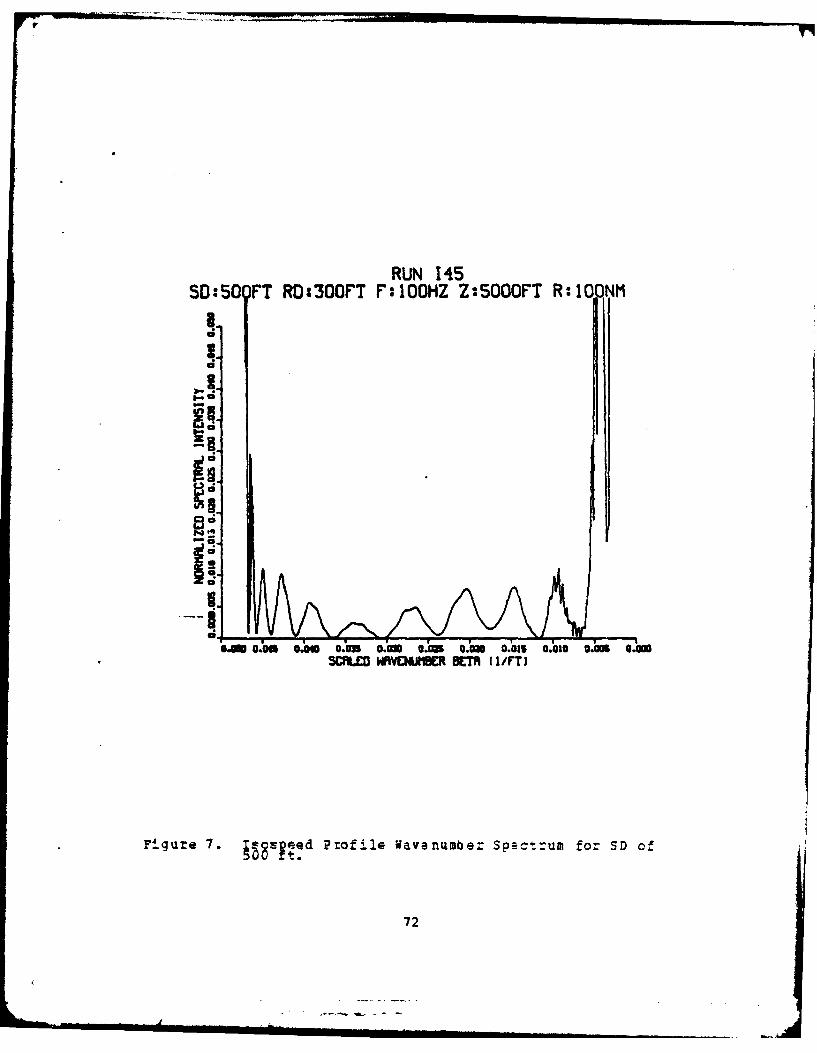
RUN 145SD:5O FT RD:300FT FI':10HZ Z:5OOOFT R:lOOt
IO
c;
C,
"mOm OwUO .m 0,2 *7 .l .I .m 40
SM ME. S I/T
Fiur . isedPoieWynme p0 tu o Do
I72

RUN 146SD:80 FT RD:300FT F:100HZ Z:5000FT R:1 NM
A
e0 d"
9.-
u.M 0.0is 0.00 Oam o.uom .m - .03S 0.019 O.as 0.0mSCFlLEO WVNUnMcR BCTh (1/FT)
Figure 8. TWesneed ?rofile Wavenumber Spz-ct:um for SD of
73

RUN 147SD:1500FT RD:300FT F:100HZ Z:5000FT R:O INM
El
-5 .0OMOM . . .n001 .1 .~
in5wvDWBn /T
Fiue960e roieWvnme Satu o Do
~7%

RUN 14850:30 OFT RD:300FT F:I00HZ Z:5000FT R:1 0 1M
..
Figure 10. gpldProfile Wvenumber spectrum for SD of
75

RUN A03SO:200FT RIJ:3OQFT F:OH Z:9000FT R:IOONI
0-
a-
~~0
a7

RUN A04SD:300rT RO:300PT F:100HZ Z:9000FT R:IOQNM
a-m eUm ao - ~a Ob .3 .00 Om *g
scmwm a 3Eaii/T
Fi ur 12 aeubrSstu fo SD f
38atz* rfl
fr.77

RUN A05SD:500FT RD:300FT F:100HZ Z:9000FT R:100NM
0 1A
&MGMaM CN OM OO . .3 .1 .w '
aCX ~aowOR(/
Fiue1. O li * rfl Wvnme pctu o Do
a7

RUN 806SD:800FT RD:300FT F:100HZ Z2900OFT R:100NM
0
0 L0
au
Fiue 4881Fi rflAvnme pctu :n Dc
I;9......

RUN 807SD:15 OFT RO:300FT F':IOOHZ Z:9000FT R:100NM
a
OU . oM 9 .06 s 0 .81 . 0 . a0 b as a. i s . n .00 0.000scILco wmvENUmBR BETA (i/rT)
Figure 15. iw tcProfile wavenumber Spectrum for SD of
80

RUN A0850:3w]OFT RD:300F*T F:IOOHZ Z:9000FT R:10 NI
Alib L II IiIIej . o . GU a.=2 a.= 0.0a5 0.=1 0.015 0.010 0.00 D.=0
SCMM.EONUJISC BETh (I /M
Figure 16. ,-6~ic Profile wavenumber spectrum for SD of
81

RUN 141SD:5OFT RD:300FT F':100HZ Z:5000FT R:100NM
a!~ a-
0 i-
C
.m .. f o a m .0 Z 0.20015 0.01 1 0. 0.25CM.CD IEMCNtC BCTm (I/FTJ
Fi gure 17. ~oeed prof-le Wavenumber Soectrum !or SD of
82

cent intensity minima, such as shown in Figs. 5 through 16.
The nulls selected for measurement were those in the middle
of the spectrum, which led to a consistent technique for
comparison and avoided the rapidly decreasing null spacing
near the left intensity maxima. The distance was measured
to the nearest 1/64 of an inch and equate! to the respective
null spacing. Thus, there is some i'heren, measurement
error. The exact null locations were difficult tc determine
in the shallow isospc.ed cases because of gentle spectrum
curvature and uncertainty in null location. The actual
profiles were very ccmplex and again the nulls were diffi-
cult to locate. One value for each spectrum plot was used
to qenerate a point on the determination curve, such as Fig.
18 for a series of riMs. The variation of the data poin-s
from the theoretical lloyd's Mirro: curve will be the normal
distance between the Foint and the curve. Measurement inac-
curacy will decrsase as source depth incrgases. This will
be significant because at shallow depth there is some varia-
tion noted from sound speed differences. The nulls ar e
well-defined at qreat depths, but there is lit'le variation
already, thus -he measurement errors w-re not considered
significant. It is possible that a numerical algorithm which
83
' '- " - -"i ii-ii i i m • ,,,

could quantitatively identify the null locations could min.-
s ize this error.
This expectation is Inferred from the wavenumber plots
by Lauer (1979) and his examinaati4on of range determination.
He found that range determination resolution increased as
the distance between source and receiver dscreased. it Is
possible that a similar relationship might exist for depth
determination. Thus greater resolution may be realized at
shallow source depth. Even at ;reater source depths the res-
olution may be acceptable for certain applications where an
approximate depth is acceptable.
The prediction curves which result from the individual
WT spectra will1 be dis-cussed in following sections. Table
III Is a listing of the predict ion curv;e comparisons which
were conducted. In the figqures only one symbol may appeaz
at a source depth if both curves had the Same null spacing
value.
841

SOURCE DEPTH DETERMINATION CURVE
C;
6-=5O A -V -30 .2 1S An '.3BMNL PFCN /
Fiue1. Eapeo ore IphDtriainCre

TABLE III
Comparison Specifications
ISOSPEED PROFILE
Figure Run Sets Constant Parameters Varying Parameter
19 11,15 R:50,F:50,RD:300 Z:10000,5000 ft
20 10,13 R:50,F:100,RD:300 Z:10000,5000 ft
21 12,16 R:100,F:50,RD:300 Z:10000,5000 ft
22 17,14 R: 100,F: 100, RD:300 Z:10000,5000 ft
23 15,16 F: 50,Z:5000, RD:300 R:50,100 nm
24 11,12 F:50,Z:10000,RD:300 R:50,100 am
25 R1,R2,R3 F: 100,Z:1000 ,RD: 300 R:25,50,75 am
26 12,17 R:100,Z:10000,RD:300 ?:100,50 hz
27 10,11 R:50,Z:10000,RD:300 F:100,50 hz
28 I118,I9 R:50, F:50,Z:10000 RD:300,800,10000 ft
REALISTIC PROFILE
Figure Run Sets Constant Parameters Varying Parameter
29 AO,BO R:100,F:100,RD:300 Space:200 nm
30 CO,DO R: 100,F:100,RD:300 Space:200 nm
31 AO,CO R:100,F:100,RD:300 Timq:20 days
32 BO,DO R: 100,F:100,RD:300 rime-20 days
33 A0,A3 F: 100,16NOV, RD:300 R:100,50 nm
34 A0,A1,A2 F: 100,16NOV, R;100 RD:300,1000,9000 ft
COMPCSIT E
Figure Run Sets Constant Parameters Varying Parameter
35 (All Isospeed and Actual Profile Run Sets)
86

B. ISOSPEED CASES
Fig. 19 is the comparison for a frequency of 50 Hz
and a range of 50 nm at water column depths of 5000 and
10,000 feet. It was not expected that there would be any
variation if the water cclumn depth was mndified, since all
bottcm interacting rays should be fully absorbed. The
curves showed excellent agreement at source depths of 800
feet and greater, but there was some variation noted for 500
feet and shallower. Some variation may be related to meas-
urement error, as noted above. Maximum variation from
'heory is observed for both lepths in the middle depth
range, approximately 500 feet, which is also the region of
greatest curvature in the source depth determination curve.
Fig. 20 is the same except the frequency has been
increased to 100 Hz. There "s better agreement from 200 to
3000 feet; however, the significance of the frequency varia-
tion has not been evaluated. Fig. 21 is for a frequency of
50 Hz and a range of 100 nm, and Fig. 22 is for 100 Hz and
100 nm. Some variaticns are noted; however, they may not be
significant, which would agree with the supposition that
87

SOURCE DEPTH OETERMINAT ION CURVEISOSPEED WRTER DEPTH VARIFITION
R:50NM r:5OflZ RO:3001?T
C!
LEEN
LLYSMRO
15a Z-SOOOrT
R
ar-t.io
a8

water column depth differences will not be significant for
an isospeed profile.
2. va !i i
Fig. 23 is the comparison for a frequency of 50 Hz
and a water column depth of 5000 feet for 50 and 100 nu.
There is essentially no difference between the curves. The
experimental curves agree well from 800 to 3000 feet, but
once again the shallow variations may result from inaccura-
cies in evaluating beta from the spectrum plots. Fig. 24 is
a similar comparison, but the water column depth has been
increased to 10,000 feet. Fig. 25 increases the frequency
to 100 Hz for ranges of 25, 50 and 75 miles. Again all
curves show very good agreement with theory, which indicates
that range variations within 10D nm of the source will prob-
ably be insignificant. Ranges beyond 100 nm were not tested
since Fitzgerald (1975) suggested that the SSFFT was not a
good approx-mation for 100 HZ beyond 111 km. This could be
tested later.
3. _ jaZi1!on
Fig. 26 is the comparison for a range of 50 nm and a
water column depth of 5000 feet for 50 and 100 Hz. Both
curves agree well with theory below 800 feet, but at 500
89

SOURCE DEPTH DETERMINATION CURVEISOSPEEO WATER DEPTH VARIATION
R:-SONl F:100IZ RD:3OOFT
El-
ci
I-LLOYDS MIIRROR
aa
BET NULUIG(/~
Fiue 0 lor~dPr5l S etrint06 ureva-. tal
09

SOURCE DEPTH DETERMINATION CURVE* ISOSPEED WATER DEPTH VARIATION
R:0100N I':5OHZ RD:3OFT
aa
BM* NUL SING& tIIRRO
Vai*,o - 12 Z.OOf
Ii O 6: Z-OO91

VAp
SOURCE DEPTH DETERMINATION CURVEASOSPEED WATER DEPTH VARIATION*R:lOONl F:iOOHZ RD:300FT
It
LEGEND-LLOYDS i I RROR
ct~a 17:t Z- I OOOFTIi a-14: Z-500IT
C!
0AA0im06aciwVia06s .M-"
BMIILSIG1/T
Figure~~~~~~ 220ogt rfl DDtriainCreia0 tUn
92

-. SOURCE DEPTH DETERMINATION CURVEISOSPEED RflNGE VARIATION
* F:5OHZ Z:5000FT RO:300FT
9
.E1
iE
LEGEND*-LLOYDS MIRRORU-15: R-50NflIi 0-15a R-IODM
e.mcio *.am a SJO OaWi 0.1 00 0.&Z5 0.0310 0.011 @.imBMT NULL SPACING II/MT
Figure 23. Isospe ,d Prof ile SD Determjination Curvg?: R
93

SOURCE DEPTH DETERMINATION CURVEISOSPEED RANGE VARIATION
ct r;5oHZ Z:1OOOOF1T RD:300FT
R
LEGCNO*-LLOYDS IIRROlt
R~ I1I: R-SOHIIa - 12: R- IOOtNl
ac
'i~a ~n06-0&s0imO;acis .ltQK0 ULSIGt/
fiue2.IoIq rfl S eam-ainCreVarihot 0
09

SOURCE DEPTH DETERMINATION CURVEISOSPEED RANGE VARIATION
F:IOOHZ Z:lOOOOFT RO:300rT
Vlt
-LEGEND
LLOYDS MIIRRORnR I: R-25NM1a-R2; R-SONlI*-R38 R-75N1
C! KC!
0.0m O aim U cion 0.,-''i0 0.i13S 0.10 0.0115 ODOM13CTR NULL SPMCZNQ* (I/rTl
Figure 25. Isospeed Profile 9D Determinatior Cuirve: RVariation - 3.
95

7 ES A O CU I UNV O NOAAD-A126
688 PRELIMINARY INVESTIGATION OF THE ENVIRONMENTAL
2/2.I SCHOOL MONTEREY CA B B STAMEY DEC 82
I FN I E

112.1111 . I 1 .
MICROCOPY RESOLUTION TEST CHART
NAMLNAL BUREAU OF STANDARDS1063A
feet the higher frequency appears to agree better. Fig. 27
extends the water column depth to 10,000 feet and there is
apparently bey-tc'; agreement with the theoretical curve.
Overall there appears to be better agreezent at 100 Hz than
at 50 Hz, but this result is not certain with the limited
number of cases run.
d4. Receiv~r RnhVrit
Fig. 28 compares receiver depths of 300, 800 and
10,000 feet for a range of 50 nm, water column depth of
10,000 feet, and frequency of 50 Hz. Again all curves agree
reasonably well. There is perhaps slightly better agreement
for the shallow receiver, but this suppositicn cannot be
verified from these limited data.
5. ARAI-il 21 _;2pee Cas
There do not appear to be any significant differ-
ences for water column depth, range, frequency or receiver
depth over the limits of variations considered. rhis was
expected since the theory is supposed to be only a function
of source depth for at isospeed profile. Thus the WT would
be expected to be equally effective for various transmis-
sion geometry patterns and frequencies, if the sound speed
profile is constant and the bottom fully absorptive. There
96

-. SOURCE DEPTH DETERMINATION CURVEISOSPEED FREOUENCY VARIATION
qt R:lOONl Z:l0000FT RO:300FT
Itt
*-LLOYDS M I RRORtR 12z r-5OHZ
a-17t r-a
a 1m
0.m cmIQ 0 ' .10 .1 .10 06f8MNL PaG(/
F Iur 26Usfedp3ieS eamlainCreV0U t o
97a

SOURCE DEPTH DETERMINATION CURVEISOSPEED FREOUENCY VARIATIONR:SI5 I Z:1OOOOFT RO:300FT
9
Iia-!LEGM4
*- LLOYDS "IIRRORi : r-SOHZ
a- 10: F-IO0HZ
0
01o w n.i 0.0 n.o 0.10 06a 06s i 0o.mo o.nm e.g.. o.ibws .bao o.ous oGom.' o~oa,' o~uw
SE NULL S ING {l/FT)
Figure 27. Iso pepd Pr file SD Determination Curve: PVarton -2 .
98

SOURCE DEPTH DETERMINATION CURVEISOSPEED RCV DEPTH VARIATION
I R:50NMl F:SOHZ Z:10000FT,
E-
9 - LLOYDS M I RROR
o-16t RO-80OFT*-19t RD-looOrr
BMT NULL SPAING (I/MT
Pigure 28. IsledProfile SD Determination Curve: RD
99

may be slight effects for receiver depth and frequency, but
these have not been substantiated.
C. REALISTIC PROFILE CASES
Fig. 29 is the comparison of spatial variability for
the curves which resulted from the spectra of profiles A and
B. (The sound speed profiles corresporiding to the pre-
diction curves will be included for each comparison.) These
were both sampled on November 16, 1980, and represent a spa-
tial separation of abcut 200 nm. Both profiles result in a
slight bias below the theoretical Lloyd's M-irror curve.
There is more variation along each curve, which is to be
expected because the profiles are not isospeed. Also, par-
tially absorbing bottoms are now used -s compared to the
fully absorbing bottoms used with the isospeed cases. The
profile and bottom effects have not yet been separated to
determine which contributes more to the departure from
theory. This would require an extensive set of intercompari-
sons between these two parameters. (The present intent is
to show that ocean variability is important.) It is diffi-
cult to differentiate between the :wo curves, but it appears
that there is a slight trend in B '::ward smaller null
100
iL

spacings. Sound speed profile B is slower than k over the
entire depth. A slower sound speed would appear to indicate
that a ray of lesser angle would be required to provide the
second arrival for the interference pattern. That would cor-
-respond to a greater vertical wavenumber and decreased beta
null spacing.
Fig. 30 compares profiles C and D, which were sam-
pled at the same locations as profiles A and B, respec-
tively, but on December 6, 1980. A similar pattern is noted
with D spacing less than C, which may again correspond to
slower sound speeds fcr profile D.
2. T ation
Fig. 31 compares profiles A and C which represent
the same location, but a separation of 20 days. There
appears to be a curve crossing at about 830 fee t , such that
spacing is less at A for sha". .i depths and greater for A
below 800 feet. The A sound spped profile is slower than the
C profile down to 800 feet aid the pattern is reversed from
800 to 2000 feet. Slower speeds appear to be related to
shorter null spacings, which appears consistent with this
example. The variaticns between the curves, however, are
quite small.
101

SOURCE DEPTH DETERMINATION CURVERCALISTIC SPATIAL VARIATIONrzlooHz R:lOONl RO:300FT
LEGMN*-LLOYDS flIMRO
0M MAL -V$ I T
RXBT CURVES
g10

SOURCE DEPTH DETERIIIN9T ION CURVEREALISTIC SPATIAL VARIATION
q F:l00HZ R:100NM RO:300FT
*LLCOS flIR.PRWrILE C*PROTILC D
..Ai 03Mu O.... a.W, 0.0100 OiA32 o.6u 0.63M 0..60BETA NULL SMAING di/rT)
AXBT CURVES
LEEN
-olw oZ0mo0fi. 60 *08-0M.
SOMN SPM (rr/SeC)
Piqure 30. S atial. vaz~ation (Z ,D): SD Determination andA BT Curvoes.
103

SOURCE:DEPTH DETERMINAITION CURVEREALS~iCTEMPORHL VARIATION* F:IOH.Z R:I10NM RD:3OFp7
* tLOYOS lIWM
S ~ n *O .1 g Jj 0 0 m 0 .0 12 5 0 .8 33 0 C A 8 0 .a
R9XBT CURVES
110

Fig. 32 presents a similar comparison for profiles B
and D. The speed profiles show almost n3 differences, except
that D is slightly slower. This result appears as a
slightly sharper deep sound channel which will mean slightly
slower velocity for the direct path. That effect may be
reflected as a slightly greater null spacing as shown.
Results for profile A waer compared for ranges of 50
and 100 nm in Fig. 33. No significant variations wer _
noted, which is similar to the results for 4 he isospeed
cases.
4. Receiver Depth Va.i ti-r
Results for profile A were also compared for
receiver depths of 300, 1000 and 9000 feet in Fig. 34.
There may be slightly better agreement for the shallow
receiver, but this is not certain.
D. COMPOSITE COMPARISON
Fig. 35 is a composite of all isospeed and actual
profile data sets. Isospeel data shDw slightly better
agreement wi:h theory; however realistic profiles ar-- a rea-
sonable apprcximation to the theoretical curve. Realistic
profile variations from the isospeed curve appear to be
105

related to the sound speed profile and different bottom
boundary conditions. The general relationships of the date.
indicate that below about 800 feet no sigaificart variations
are noted. Specific curves will apparently provide better
predictions at shallower depths. It may be sufficient fcr
certain applications to provldg climatological or theoreti-4
cal predictict curves. These curves could be enhanced or
modified by updated curves thit would rzeflect the current
sound speed profil4e.
106

....
SOURCE DEPTH DETERMINATION CURVEREALISTIC TEMPORAL VARIATION.:1OOHZ R:IOONM RO:30OFT
LEGEND- LLOYDS IIRROR
* - PROFILE 13-- * a-PROFILE O
0- S
E - URrL 0
0.m AW .WS .& j0.6a 0.6150 0.61n 0.0,20. o.u s.u. o.7, ~i o e m .l ~
BE NULL SPCING I I/T
RXBT CURVES
LEGENDo,
IiL.O 4.0 , . O 48. 4 0 4NO.0 490.0 4910.0 4W.0 4=10.a 4940.0SOUND SPEED (f"T/SCJ
Figure 32. Temporal Variation (B,D: SD Determinati"n andAXET Curves.
107
7-

SOURCE DEPTH DETERMINA~TION CURVEREBLISTIC RANGE VARIATION
* r:100HZ R0:300FT
AO-RMQE:C IMNMf
Ii __ ___
sAc. on 9.imc 0.60ms 0. a.i 0.8,150 0.617s 0.0=BETA NULL SPRtCING (1/rT)
Figure 33. Range (R) Variatijon for Profile A.
108a

SOURCE DEPTH DETERMINATION CURVEREALISTIC RCV DEPTH VARIATION
F:IOOHZ R:100NM
I * - LLOYDS IIMMOo-A-RCV OEM&h:OOFrT
GE* - R2-RCV OCPml9OOOF"r
E-
LmU 0.00 0.in0 O.hWs 0.03Wa Oita 0.60 0.0315 0.UODBETA NULL SM'lING (1/F?)
Figure 34i. Receiver Depth (RD) Variation for P~ofile A.
109

SOURCE DEPTH DETERMIINATION CURVE
ASOSPEED AND REALISTIC CASES
qt
LECND* =LYDS IIIRRR
ii o - REMISTIC PROILES
a 0 =
km am m 90 AWSclo0iuGZo0in008o M a JLS O r
Figure 35. Ca ast Cmario foussedan elsaCasts.

V. . I2_ oA
The Wavenumber Technique (UT), as proposed by Lauer
(1979) has been investigated for source depth determination.
Several idealized and actual scenarios of oceanic and acous-
tic parametric variations were tested. rhere is excellent
agreement between the ideal test cases and the theoretical
Lloyd's Mirror effect. The realistic zases showed signifi-
cant similarity as well, but with some bias toward smaller
wavenumber spacing. This is qualitatively attributed to
sound speed profile variations in the water and sediment.
There appears to be a response of the VT to variations
in input, which is beneficial in allowing evaluation of the
relative importance of individual parameters. changes in
range and water column depth do not indicate any significant
variation. Some differences are possibly suggested fo:
receiver depth and frequency, but the results have not been
fully analyzed. The WT appears to respond well to changes
in the environmental paramete rs, such as sound speed
profile. This is seen from the average bias of the actual
cases from the isospeed cases. The bias does appear to be
111

relatively consistent and shows the importance of oceanic
variations in both space and in time. Thus, it appears that,
if information is available for the bottom structure, and if
a realistic sound speed profile can be generated, then a
very specific family of curves could be generated for vari-
ous frequency and receiver depth combinations. This simplic-
ity indicates possible operaticnal applicability and
flexibility.
These are the first known source depth determination
curves for the WT and thus there. is no comparison available.
It may be that there are some biases in these curves which
would be discovered vhen comparative runs are made using
other inputs or propagation models. Comparison with observed
signals might also reveal biases that arS related to the IT
or to the propagation model. An explanation has not been
determined for the U-shape nature of the wavenumber spectrum
plots and thus slightly different curves might result if
this is found to bias the null spacing. Also there is a
bias associated with the method of manually estimating the
null spacing. This might be resolved with a computer proce-
dure to locate the nulls. The experimental curves actually
agree well with thecry under the assumption of a flat,
112

totally-reflectinq surface and a fully-absorbing bottom.
The premise that the theory might be approximately accurate
"n realistic cases appears valid. This overall generally
smooth fit supports th" validity of the Ur.
This has been an initial investigation of the WT, and
thus only a broadbrush study was possible. These prelimi-
nary results indicate that additional analysis might be ben-
eficial. The response of the WT to input from different
propagation models would deteraine if results from different
models could be compared. Detailed investigation of the sp.-
cific effects of various parameters would lead to a quar.ti-
tative analysis of the sensitivity of the WT. An explanation
for the amomalous U-shaped spetrum and the development of
an algorithm which can accurately determine null locations
would be necessary before the WT could be used practically.
An extremely important investigation would be the ccmpar-son
of analyzed actual signals to predictions from the WT ".o
determine applicability, accuracy, consistency and any
appropriate biases.
The intett of this research was to datermine the valid-
ity of the WT by development of source !epth determina-:_cn
curves and to evaluate the oceanic and acoustic
113

71sensitivities of these curves. The results obtained indicate
that in general the wT appears to be valil vi'h respect to
the Lloyd's Mirror effect. The parametri-c variations which
were investigated show that oceanic variability is extremely
important, but that the VT is flexible for other parameters,
such as transmission geometry. The WT appears to be viable
for operational applications. rhe additiDnal investigationls
suggested above would determina the valility of this suppo-
sition. it is conceivable that the WT zould be developed
inoan operational p~ediction product.
11(4
LIST OF REFERENCES
Brock, U.K., Buchal, B°N., and S pofford, :.V. "Modifying theSound Speed Proile t oIprove the &ccuraIy oi theParabolic-E uation Technmque," . .rv. 62,p. 543-552, eptember 197
DeSanto J.A., "Relation between the Solutions of theHelmholtz and Parabolic Equaqions or Sound PDagation," J.Io ° 22g. k&., v. E2. p. 29- 297, August 1577.
DeSanto, J°A. Perkins, J.S., and Baer, R.N., "A Correctionto the Parabolic Approximation,- J. !42o . oc. j., v. 6,p. 1664-1666, December 1978.
DiNapoli, F.R. and Deavenport, R.L., "Numerical Models ofUnderwater Acoustic Propagation in Ocean A ic, ed. byJ.A. DeSanto, Springer- erlag, i979, p. 71- T3.
Dunlap, C.R., "Naval Postgraduate School ASTREXMeasurements," (Unpublished), 1982.
Fitz erald M "elmholtz Equation as in Initial ValueProblem with Application to Acoustic Propagation," J.Acou§t. So. ja., v. 57, p. 839-842, April 1975.
Hardin, R.H. and Tappert, F.D., "Applications of the Split-Step Fourier Method to the Numerical Solution of onlinearand Variable Coefficient Wave Equation," SA i v. 15,p. 423, 1973.
Kinsler, L.E., Frey, A.R., Coppens, A.B. and Sanders, J.V.,Th . _ Edition, John Wiley mnd
Lauer R B Personal communication to B.B. Stamey onOctober2
Luer, R.B. (21 Personal communication to B.B. Stamey onDecem6 er 16, 192.
Lee D., Botseas G. and Papadakis, J.S., "Finite-Difference Solut~on ¢ the P~ rabolice Wave Equation," J.
o joc. 22 ., v. 70, p. 795- 800, September 1981. -
Leontovich, M.A. and Pock, V.A., "Solution of the Problem ofPropagation of Electrcmagnetic Waves alon; the Earth'sSurface by the Method of Parabolic Equation," J. Phls° 2fg...1, v. 10, p. 13, 1946.
McDaniel, S.T. (I), "ProPa ation of Normal mode in theI abolic Approximatin,"l . _kc2_. §o;- I&_., v- 57, p.S C311, Fe ruary 19 5. 11.
115

McDaniel, S.T. (2) , "Parabolic Approximations for UnderwaterSo~d Popatin p i jjj, v. 58, p.1179-185,Dectmber 141--5!C
McDaniel S.T. and Lee, D. "A Finite-Difference Treatmentof Interlace Condit5.ons for the Parabolic Wave Ejuati.on: The
855-858, April 1982.
Naval Air Development Center Report NADC-72001-AE, Nojjai1
rq.!5aC~ ~ITaferger an WLU. XKW ar-W-TPrl-Tg7.
Naval Oceanographic Office Reference Publication 16,of--adA oor fe-177 t 1_ _~hast Pacific by W.T.
Naval Ocean Research and Development Activity Technical Note12,~ tijAXn M ofl, by H. . B rock,
January, 19-78.
Naval Underwater Systems Center Technical. Report 4103, FastF!1dt~&4 I"Mutilaered t31ied b .R. DiNapoli., 26
Naval Underwater Systems Center Technical Memorandum 771160,The 1je7se Zast F Id Progra (IE): Ap licati.on to th
Naval Underwater Systems Center Technical Report 4s887-1,Ster Acoust a O d r 9cean Strtified
Naval Underwater. Systems Center Technical Memorandum 791105,j.j" jpaxim.- ill 11-e la-a e 2231;n, by R.B. Lauer,
Naval. Underwater Systems Center TechnicalReport 5929,E~lli.3 1~t kd 3 Iptdl WHAb t ion
Naval Underwater Systems Center Technical Repor* 6659, 1FD:
Lzqa u Taiff, girgI -G, t . -
Officer, C.E.,.,:n_ odution to the jh~o~j of Sound
Palmer, D.R., "Eikonal Approximation- and tht ParabolicEquation," . So.jv.60, p. 343-354, August
116

Tappert, F.D., "The Parabolic Approximation method 11 in Wqyean ~ d. by J.B. ielleranM
Tatro " P.R. Communication to Rowland M. Stevens, The JohnsHopkins University, on April 20, 1977.
Thorp, W.H. "Analytic Description of 'the Low FrequencyAttenuatio; Coefficient," t . 0. ji., v. 42, p .270,July 1967.KaM
ftcGrav-Hill, ini
Urick, R.J.o,I2Z pLg4q-aton in the SeA, Defense AdvancedResearch P oects Ag encyr7~
117

INITIAL DISTRIBUTION LIS?
No. Copies
1. Defense Technical Information Center 2Cameron StationAlexandria, VA 22314
2. Suerintendent 2At ni Library a Cede_0.142Naval Post rahaae schoolMonterey, 9A 93940
3. Super intendent 1Attn: Professor C.N.K. Eooers, Code 68Naval Postgraduate SchoolMonterey, CA 93940
4. Superintendent 1Att n: Professor R.J. Renard, Code 53Naval Postgraduate SchoolMonterey, CA 93940
5. Superintendent 3Attn: Associate Professor A.B. Coppens, Code 61Naval Postgraduate SchoolMonterey, CA 93940
6. Superintendent 3Atn: LCDR C.R.u Dunlap, (Rat), Cde 68Naval Postqraduate SchoolMonterey, CA 93940
7. Commanding Officer INaval Ocean Research and Development Act.vityNSTL StationBay St. Louis, MS 39522
8. Commanding Officer 2Attni Mr. R.B. Lauer, Code 323Naval Ocean Research and Development ActivityNSTL StationBay St. Louis, HS 39522
9. Commanding Officer 2Attn* Mr. T.N. Lawrence, Code 323Naval Ocean Research anA Development ActivityNSTL StationBay St. Louis, MS 39522
10. Commanding Officer IAttn* Code 520Naval Ocean Research and Development ActivityNSTL StationBay St. Louis, MS 39522
118
4

11. Commanding f~ekttn, CDR H5. 5C:C iist.N IO tSN Code 522ial ocean Research an Development ActivityWSTL StationBay St. Louls, HS 39522
12. LT B.fl. Stamey Jr 45508 Buskirk r etWorth Char eston, SC 29406
1 19
