prediction of shrinkage of individual parameters using the...
TRANSCRIPT

Prediction of shrinkage of individual parameters using
the Bayesian information matrix in nonlinear mixed-effect
models with application in pharmacokinetics
F. Combes (1,2,3)
S. Retout (2), N. Frey (2) and F. Mentré (1)
PODE 2012
(1) INSERM, UMR 738, Univ Paris Diderot, Sorbonne Paris Cité, Paris, France
(2) Pharma Research and Early Development, Translational Research Sciences,
Modeling and Simulation, F. Hoffmann-La Roche ltd, Basel, Switzerland
(3) Institut Roche de Recherche et Médecine Translationnelle, Boulogne-Billancourt, France
3/23/2012

Outline
1. Context
2. Objectives
3. Materials and methods
4. Results
5. Conclusion & perspectives
2
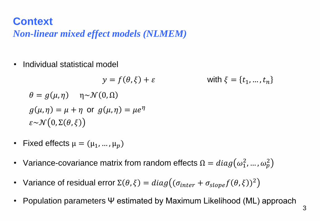
• Individual statistical model
𝑦 = 𝑓 𝜃, 𝜉 + 𝜀 with 𝜉 = 𝑡1, … , 𝑡𝑛
𝜃 = 𝑔 𝜇, 𝜂 η~𝒩 0, Ω
𝑔 𝜇, 𝜂 = 𝜇 + 𝜂 or 𝑔 𝜇, 𝜂 = 𝜇𝑒𝜂
𝜀~𝒩 0, Σ 𝜃, 𝜉
• Fixed effects µ = (µ1, … , µ𝑝)
• Variance-covariance matrix from random effects Ω = 𝑑𝑖𝑎𝑔 𝜔12, … , 𝜔𝑝
2
• Variance of residual error Σ 𝜃, 𝜉 = 𝑑𝑖𝑎𝑔 (𝜎𝑖𝑛𝑡𝑒𝑟 + 𝜎𝑠𝑙𝑜𝑝𝑒𝑓 𝜃, 𝜉 )2
• Population parameters Ψ estimated by Maximum Likelihood (ML) approach
Context Non-linear mixed effect models (NLMEM)
3
4
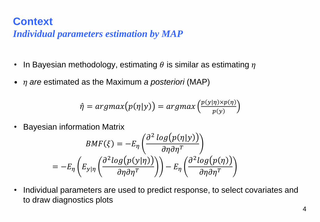
• In Bayesian methodology, estimating 𝜃 is similar as estimating 𝜂
• 𝜂 are estimated as the Maximum a posteriori (MAP)
𝜂 = 𝑎𝑟𝑔𝑚𝑎𝑥 𝑝 𝜂|𝑦 = 𝑎𝑟𝑔𝑚𝑎𝑥𝑝 𝑦|𝜂 ×𝑝 𝜂
𝑝 𝑦
• Bayesian information Matrix
𝐵𝑀𝐹 𝜉 = −𝐸𝜂
𝜕2 𝑙𝑜𝑔 𝑝 𝜂|𝑦
𝜕𝜂𝜕𝜂𝑇
= −𝐸𝜂 𝐸𝑦|𝜂
𝜕2𝑙𝑜𝑔 𝑝 𝑦|𝜂
𝜕𝜂𝜕𝜂𝑇− 𝐸𝜂
𝜕2𝑙𝑜𝑔 𝑝 𝜂
𝜕𝜂𝜕𝜂𝑇
• Individual parameters are used to predict response, to select covariates and
to draw diagnostics plots
Context Individual parameters estimation by MAP
Context Shrinkage
5
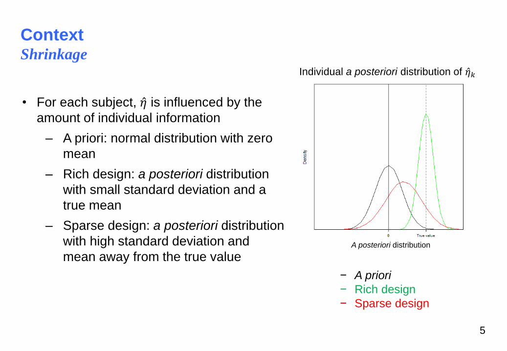
− A priori
− Rich design
− Sparse design
• For each subject, 𝜂 is influenced by the
amount of individual information
‒ A priori: normal distribution with zero
mean
‒ Rich design: a posteriori distribution
with small standard deviation and a
true mean
‒ Sparse design: a posteriori distribution
with high standard deviation and
mean away from the true value
Individual a posteriori distribution of 𝜂 𝑘
A posteriori distribution
6
Context
Observed shrinkage
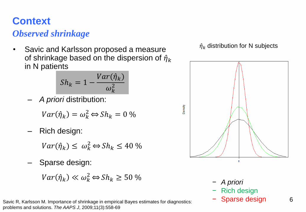
• Savic and Karlsson proposed a measure of shrinkage based on the dispersion of 𝜂 𝑘 in N patients
– A priori distribution:
𝑉𝑎𝑟 𝜂 𝑘 = 𝜔𝑘2 𝑆ℎ𝑘 = 0 %
– Rich design:
𝑉𝑎𝑟(𝜂 𝑘) ≤ 𝜔𝑘2 𝑆ℎ𝑘 ≤ 40 %
– Sparse design:
𝑉𝑎𝑟 𝜂 𝑘 ≪ 𝜔𝑘2 𝑆ℎ𝑘 ≥ 50 %
𝑆ℎ𝑘 = 1 −𝑉𝑎𝑟(𝜂 𝑘)
𝜔𝑘2
𝜂 𝑘 distribution for N subjects
Savic R, Karlsson M. Importance of shrinkage in empirical Bayes estimates for diagnostics:
problems and solutions. The AAPS J, 2009;11(3):558-69
− A priori
− Rich design
− Sparse design
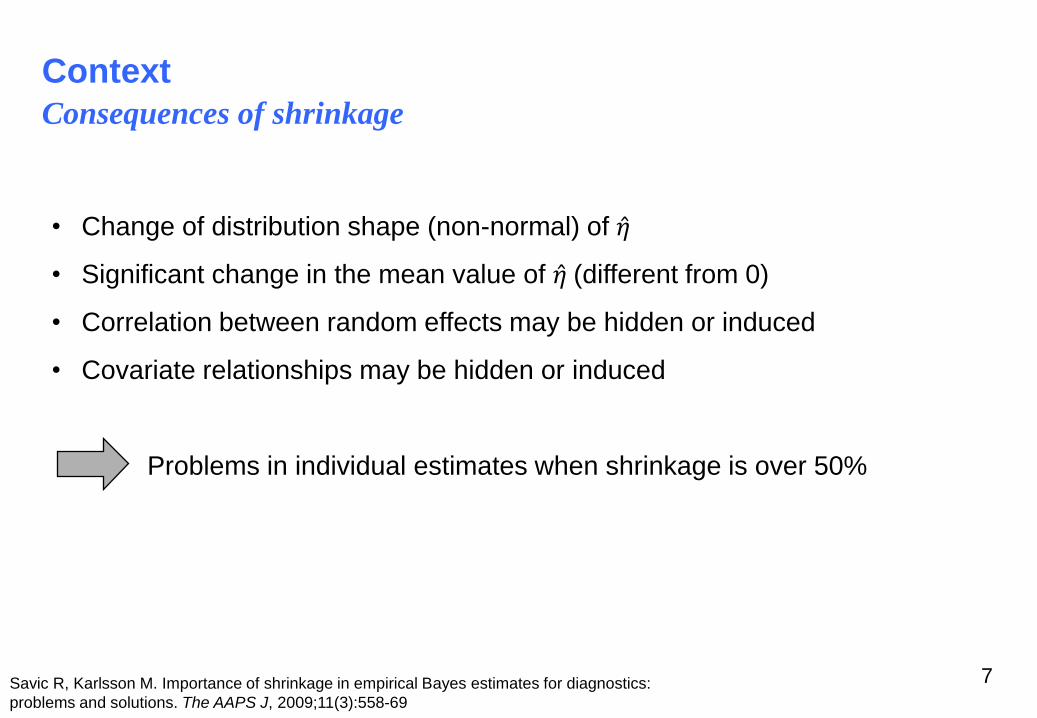
• Change of distribution shape (non-normal) of 𝜂
• Significant change in the mean value of 𝜂 (different from 0)
• Correlation between random effects may be hidden or induced
• Covariate relationships may be hidden or induced
Problems in individual estimates when shrinkage is over 50%
Context
Consequences of shrinkage
7 Savic R, Karlsson M. Importance of shrinkage in empirical Bayes estimates for diagnostics:
problems and solutions. The AAPS J, 2009;11(3):558-69
Objectives
Approximate BMF using first-order linearization
Describe relationship between BMF and shrinkage
Evaluate by simulation BMF and link with shrinkage
8

Materials and methods Design evaluation and optimization in NLMEM
• Design evaluation and optimization based on Rao-Cramer inequality:
𝑀𝐹−1 is the lower bound of estimation variance
• Individual estimation: Individual Fisher information Matrix
IMF 𝜃, 𝜉 = 𝐹 𝜃, 𝜉 𝑇Σ 𝜃, 𝜉 −1𝐹 𝜃, 𝜉
with 𝐹 𝜃, 𝜉 =𝜕𝑓 𝜃,𝜉
𝜕𝜃𝑇
• Population estimation: Population Fisher information Matrix (PMF)
– evaluated using First-Order linearization (FO)
– implemented in R in PFIM 3.2
9 Retout S, Mentré F, Bruno R. Fisher information matrix for non-linear mixed-effets models: evaluation and application for optimal design
of enoxaparin population pharmacokinetics. Stat Med, 2002;21:2623-39

Materials and methods Bayesian design evaluation
• Bayesian estimation of individual random effects
• Two methods
– Simulate 𝜂 to compute 𝐸𝜂 by Monte-Carlo simulation (MC)
– FO
• for additive random effects
BMF 𝜉 = 𝐹 µ, 𝜉 𝑇Σ µ, 𝜉 −1𝐹 µ, 𝜉 + Ω−1
• for exponential random effects
BMF 𝜉 = Μ𝑇𝐹 µ, 𝜉 𝑇Σ µ, 𝜉 −1𝐹 µ, 𝜉 Μ + Ω−1
with Μ = diag(µ1, … , µ𝑝)
Merlé Y, Mentré F. Bayesian design criteria: computation, comparison and application to a pharmacokinetic and a
pharmacodynamic model. J Pharmacokinet Biopharm, 1995;23(1):101-25
10
𝐵𝑀𝐹 𝜉 = 𝐸𝜂 𝐼𝑀𝐹 𝑔 µ, 𝜂 , 𝜉 + Ω−1
Materials and methods Shrinkage in linear mixed effects model
11
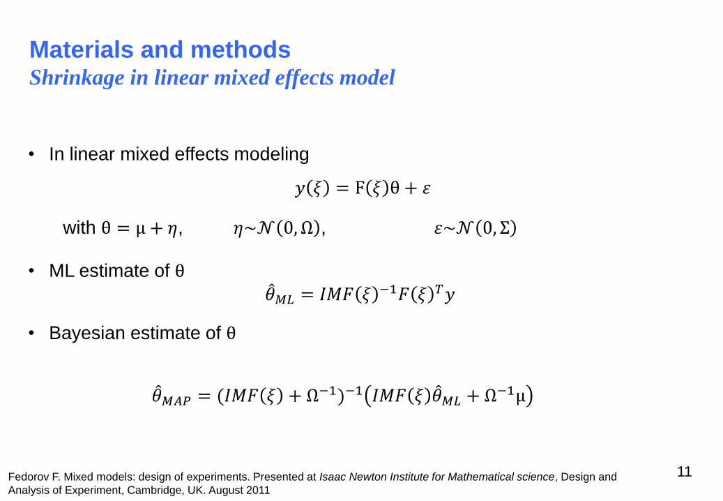
• In linear mixed effects modeling
𝑦 𝜉 = F 𝜉 θ + 𝜀
with θ = µ + 𝜂, 𝜂~𝒩 0, Ω , 𝜀~𝒩 0, Σ
• ML estimate of θ 𝜃 𝑀𝐿 = 𝐼𝑀𝐹 𝜉 −1𝐹 𝜉 𝑇𝑦
• Bayesian estimate of θ
𝜃 𝑀𝐴𝑃 = (𝐼𝑀𝐹 𝜉 + Ω−1)−1 𝐼𝑀𝐹 𝜉 𝜃 𝑀𝐿 + Ω−1µ
Fedorov F. Mixed models: design of experiments. Presented at Isaac Newton Institute for Mathematical science, Design and
Analysis of Experiment, Cambridge, UK. August 2011
Materials and methods Shrinkage in nonlinear mixed effects model
12
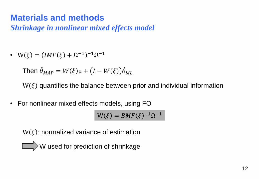
• W 𝜉 = 𝐼𝑀𝐹 𝜉 + Ω−1 −1Ω−1
Then 𝜃 𝑀𝐴𝑃 = 𝑊 𝜉 µ + 𝐼 − 𝑊 𝜉 𝜃 𝑀𝐿
W 𝜉 quantifies the balance between prior and individual information
• For nonlinear mixed effects models, using FO
W 𝜉 : normalized variance of estimation
W used for prediction of shrinkage
W 𝜉 = 𝐵𝑀𝐹 𝜉 −1Ω−1
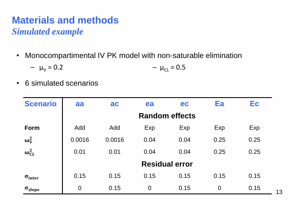
Materials and methods Simulated example
• Monocompartimental IV PK model with non-saturable elimination
– µV = 0.2 ─ µCL = 0.5
• 6 simulated scenarios
13
Scenario aa ac ea ec Ea Ec
Random effects
Form Add Add Exp Exp Exp Exp
𝛚𝐕𝟐 0.0016 0.0016 0.04 0.04 0.25 0.25
𝛚𝐂𝑳𝟐 0.01 0.01 0.04 0.04 0.25 0.25
Residual error
𝛔𝐢𝐧𝐭𝐞𝐫 0.15 0.15 0.15 0.15 0.15 0.15
𝛔𝐬𝐥𝐨𝐩𝐞 0 0.15 0 0.15 0 0.15

Materials and methods Design
14
• Several designs from 2 to 5 samples
- {0.05, 0.15, 0.3, 0.6, 1}
- {0.05, 0.3, 0.6, 1}
- {0.05, 0.3, 0.6}
- {0.05, 0.3}
• For each scenario, 1000 subjects with the
same design simulated
• Population parameters fixed to their true
value
• Estimation of individual parameters by MAP
with NONMEM 7. and MONOLIX 4.0

Materials and methods Shrinkage investigation
• Exploration of scatterplots of individual estimates from NONMEM vs
simulated parameters along with observed shrinkage
• Evaluation of the approximation of BMF by MC and FO
• Prediction of W from BMF
• Comparison of W vs observed shrinkage with NONMEM and MONOLIX
NB: Results presented for clearance
15
Validation of BMF computation and shrinkage
16
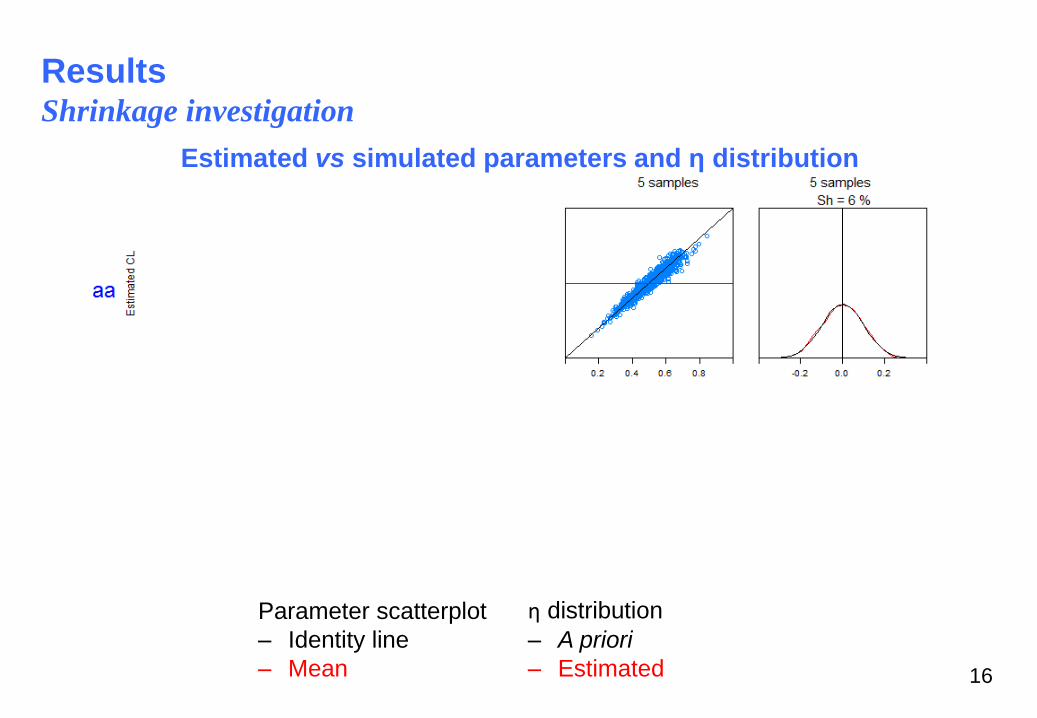
Results Shrinkage investigation
Estimated vs simulated parameters and η distribution
Parameter scatterplot
‒ Identity line
‒ Mean
η distribution
‒ A priori
‒ Estimated
17
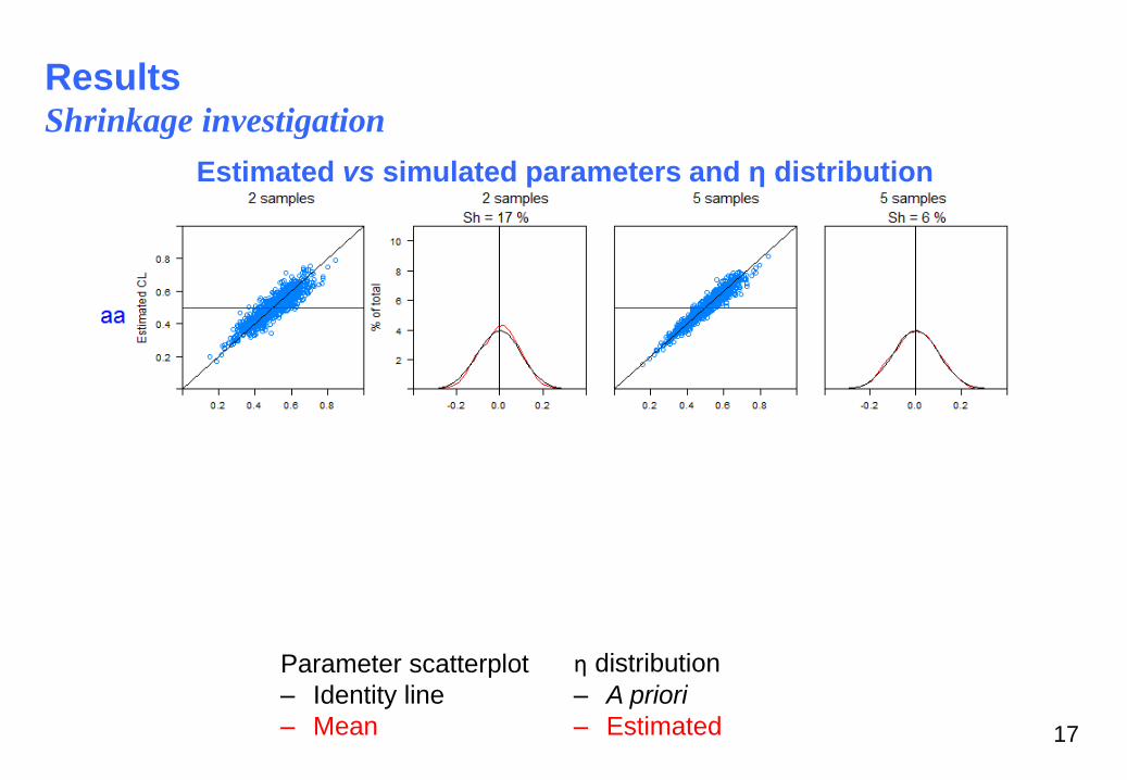
Results Shrinkage investigation
Estimated vs simulated parameters and η distribution
Parameter scatterplot
‒ Identity line
‒ Mean
η distribution
‒ A priori
‒ Estimated

18
Results Shrinkage investigation
Estimated vs simulated parameters and η distribution
Parameter scatterplot
‒ Identity line
‒ Mean
η distribution
‒ A priori
‒ Estimated

19
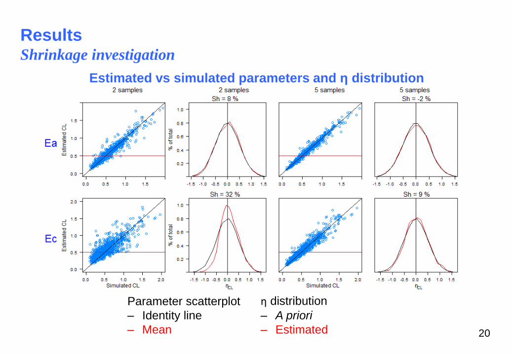
Results Shrinkage investigation
Estimated vs simulated parameters and η distribution
Parameter scatterplot
‒ Identity line
‒ Mean
η distribution
‒ A priori
‒ Estimated
20
Results Shrinkage investigation
Estimated vs simulated parameters and η distribution
Parameter scatterplot
‒ Identity line
‒ Mean
η distribution
‒ A priori
‒ Estimated
Results BMF approximation
21
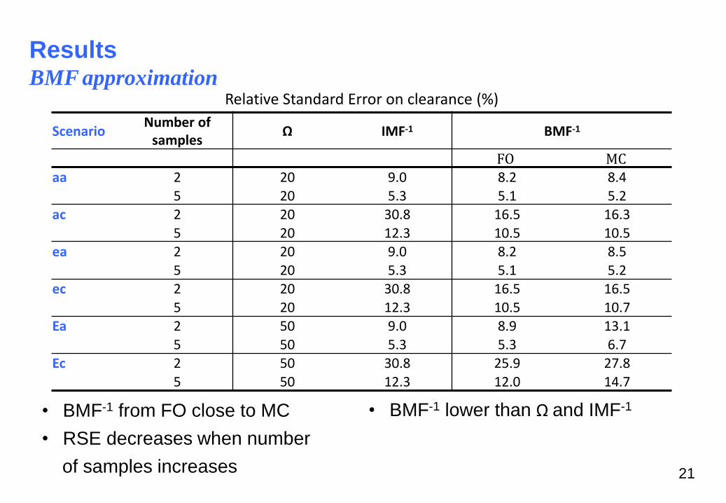
Relative Standard Error on clearance (%)
Scenario Number of
samples Ω IMF-1 BMF-1
FO MC
aa 2 20 9.0 8.2 8.4 5 20 5.3 5.1 5.2
ac 2 20 30.8 16.5 16.3 5 20 12.3 10.5 10.5
ea 2 20 9.0 8.2 8.5
5 20 5.3 5.1 5.2
ec 2 20 30.8 16.5 16.5
5 20 12.3 10.5 10.7
Ea 2 50 9.0 8.9 13.1
5 50 5.3 5.3 6.7 Ec 2 50 30.8 25.9 27.8
5 50 12.3 12.0 14.7
• BMF-1 from FO close to MC
• RSE decreases when number
of samples increases
• BMF-1 lower than Ω and IMF-1
Results BMF approximation
22
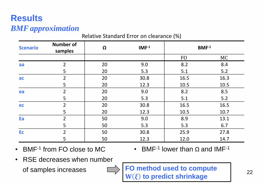
Relative Standard Error on clearance (%)
Scenario Number of
samples Ω IMF-1 BMF-1
FO MC
aa 2 20 9.0 8.2 8.4 5 20 5.3 5.1 5.2
ac 2 20 30.8 16.5 16.3 5 20 12.3 10.5 10.5
ea 2 20 9.0 8.2 8.5
5 20 5.3 5.1 5.2
ec 2 20 30.8 16.5 16.5
5 20 12.3 10.5 10.7
Ea 2 50 9.0 8.9 13.1
5 50 5.3 5.3 6.7 Ec 2 50 30.8 25.9 27.8
5 50 12.3 12.0 14.7
• BMF-1 from FO close to MC
• RSE decreases when number
of samples increases
• BMF-1 lower than Ω and IMF-1
FO method used to compute
𝐖 𝝃 to predict shrinkage

Results Shrinkage prediction
23
• Similar values of observed shrinkage with NONMEM and
MONOLIX
• Scatterplot close to the identity line
Predicted vs observed shrinkage
Scenarios
■ aa
■ ac
■ ea
■ ec
■ Ea
■ Ec

Conclusion
24
• Shrinkage influenced by
– number of samples
– error model
– variability of parameters
• Shrinkage reflects distortions in 𝜂 distribution
• Computation of BMF by FO adequate
• New formula to predict shrinkage from BMF
Perspectives
25
• Further evaluations are needed on more “extreme” models: high variances of
random effects or high residual error
• Ongoing developments on a more complex Target-Mediated Drug Disposition
model
• Use of BMF for individual design optimization for MAP
Frey N, Grange S, Woodworth T. Population pharmacokinetics analysis of tocilizumab in patients with rheumatoid arthritis. J
Clin Pharmacol, 2010;50(7):754-66

Backup slides
26

27
Results Shrinkage investigation
Estimated vs simulated parameters and η distribution
Parameter scatterplot
‒ Identity line
‒ Mean
η distribution
‒ A priori
‒ Estimated

28
Results Shrinkage investigation
Estimated vs simulated parameters and η distribution
Parameter scatterplot
‒ Identity line
‒ Mean
η distribution
‒ A priori
‒ Estimated
29
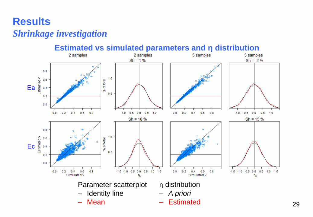
Results Shrinkage investigation
Estimated vs simulated parameters and η distribution
Parameter scatterplot
‒ Identity line
‒ Mean
η distribution
‒ A priori
‒ Estimated
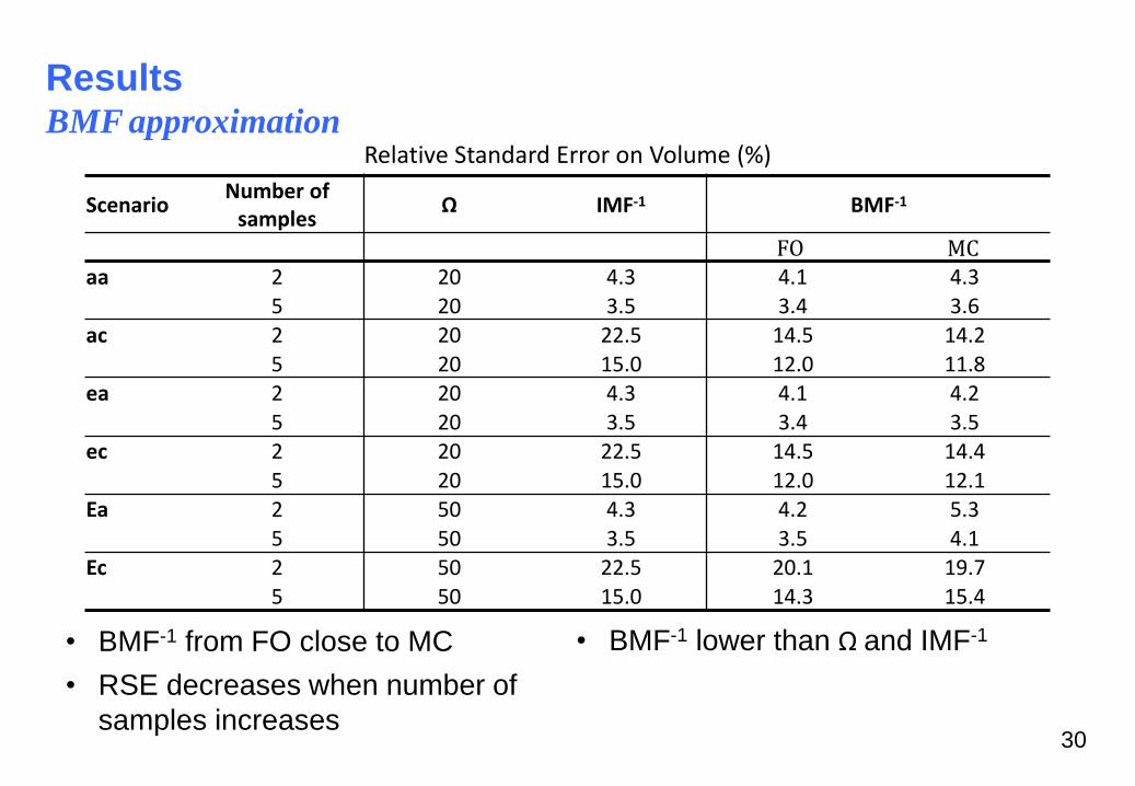
Results BMF approximation
30
Relative Standard Error on Volume (%)
Scenario Number of
samples Ω IMF-1 BMF-1
FO MC
aa 2 20 4.3 4.1 4.3 5 20 3.5 3.4 3.6
ac 2 20 22.5 14.5 14.2 5 20 15.0 12.0 11.8
ea 2 20 4.3 4.1 4.2
5 20 3.5 3.4 3.5
ec 2 20 22.5 14.5 14.4
5 20 15.0 12.0 12.1
Ea 2 50 4.3 4.2 5.3
5 50 3.5 3.5 4.1 Ec 2 50 22.5 20.1 19.7
5 50 15.0 14.3 15.4
• BMF-1 from FO close to MC
• RSE decreases when number of
samples increases
• BMF-1 lower than Ω and IMF-1

Results Shrinkage prediction
31
• Similar values of observed shrinkage with NONMEM and
MONOLIX
• Scatterplot close to the identity line
Predicted vs observed shrinkage
Scenarios
■ aa
■ ac
■ ea
■ ec
■ Ea
■ Ec
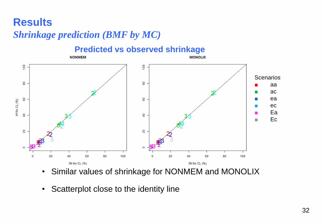
Results Shrinkage prediction (BMF by MC)
32
• Similar values of shrinkage for NONMEM and MONOLIX
• Scatterplot close to the identity line
Scenarios
■ aa
■ ac
■ ea
■ ec
■ Ea
■ Ec
Predicted vs observed shrinkage
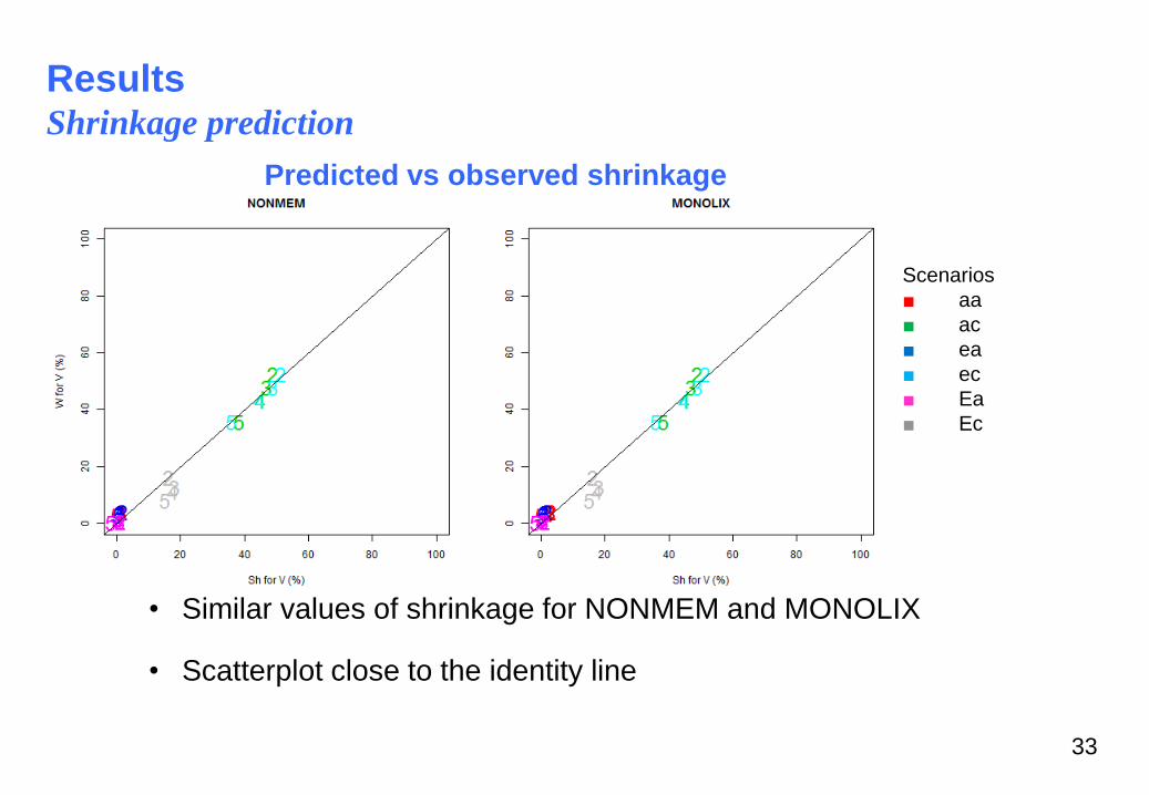
Results Shrinkage prediction
33
• Similar values of shrinkage for NONMEM and MONOLIX
• Scatterplot close to the identity line
Scenarios
■ aa
■ ac
■ ea
■ ec
■ Ea
■ Ec
Predicted vs observed shrinkage

Results Shrinkage prediction (BMF by MC)
34
• Similar values of shrinkage for NONMEM and MONOLIX
• Scatterplot close to the identity line
Scenarios
■ aa
■ ac
■ ea
■ ec
■ Ea
■ Ec
Predicted vs observed shrinkage
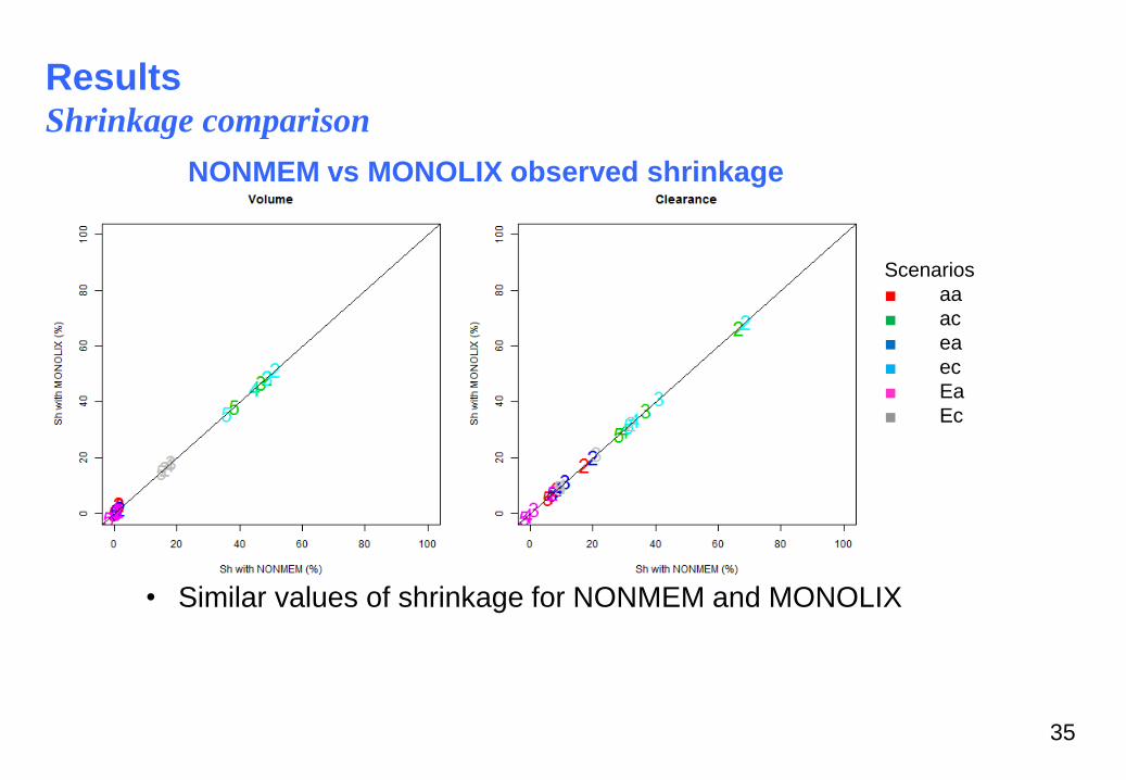
Results Shrinkage comparison
35
• Similar values of shrinkage for NONMEM and MONOLIX
Scenarios
■ aa
■ ac
■ ea
■ ec
■ Ea
■ Ec
NONMEM vs MONOLIX observed shrinkage