HAL Id: hal-01502419https://hal.archives-ouvertes.fr/hal-01502419

Submitted on 5 Apr 2017

HAL is a multi-disciplinary open accessarchive for the deposit and dissemination of sci-entific research documents, whether they are pub-lished or not. The documents may come fromteaching and research institutions in France orabroad, or from public or private research centers.

L’archive ouverte pluridisciplinaire HAL, estdestinée au dépôt et à la diffusion de documentsscientifiques de niveau recherche, publiés ou non,émanant des établissements d’enseignement et derecherche français ou étrangers, des laboratoirespublics ou privés.

Prediction and control of combustion instabilities in realengines

Thierry Poinsot

To cite this version:Thierry Poinsot. Prediction and control of combustion instabilities in real engines. Proceedings ofthe Combustion Institute, Elsevier, 2017, vol. 36 (n° 1), pp. 1-28. �10.1016/j.proci.2016.05.007�.�hal-01502419�

To link to this article : DOI: 10.1016/j.proci.2016.05.007 URL : http://dx.doi.org/10.1016/j.proci.2016.05.007

This is an author-deposited version published in: http://oatao.univ-toulouse.fr/ Eprints ID: 17713

Open Archive Toulouse Archive Ouverte (OATAO)

OATAO is an open access repository that collects the work of Toulouse researchers and makes it freely available over the web where possible.

To cite this version: Poinsot, Thierry Prediction and control of combustion instabilities in real engines. (2017) Proceedings of the Combustion Institute, vol. 36 (n° 1). pp. 1-28. ISSN 1540-7489

Any correspondence concerning this service should be sent to the repository administrator: staff-oatao@listes-diff.inp-toulouse.fr

Prediction and control of combustion instabilities in real

engines

T. Poinsot a , b , c , ∗

a IMF Toulouse, INP de Toulouse and CNRS, Toulouse 31400, France b CERFACS, Toulouse 31057, France

c Center for Turbulence Research, Stanford, CA 94305, USA

Abstract

This paper presents recent progress in the eld of thermoacoustic combustion instabilities in propulsion en- gines such as rockets or gas turbines. Combustion instabilities have been studied for more than a century in simple laminar con gurations as well as in laboratory-scale turbulent "ames. These instabilities are also encountered in real engines but new mechanisms appear in these systems because of obvious differences with academic burners: larger Reynolds numbers, higher pressures and power densities, multiple inlet systems, complex fuels. Other differences are more subtle: real engines often feature speci c unstable modes such as azimuthal instabilities in gas turbines or transverse modes in rocket chambers. Hydrodynamic instability modes can also differ as well as the combustion regimes, which can require very different simulation models. The integration of chambers in real engines implies that compressor and turbine impedances control instabil- ities directly so that the determination of the impedances of turbomachinery elements becomes a key issue. Gathering experimental data on combustion instabilities is dif cult in real engines and large Eddy simulation (LES) has become a major tool in this eld. Recent examples, however, show that LES is not suf cient and that theory, even in these complex systems, plays a major role to understand both experimental and LES results and to identify mitigation techniques.

Keywords: Instabilities; LES; Thermoacoustics; Gas turbines

1. Introduction

Most combustion systems are designed to oper- ate in stable regimes. However, all experimentalists

∗ Correspondence to: IMF Toulouse, INP de Toulouse

and CNRS, 31400 Toulouse, France

E-mail address: thierry.poinsot@cerfacs.fr

working on steady combustion chambers (furnaces, gas turbines, power plants) know that ’sometimes’, a chamber starts exhibiting unexpected oscillations. These combustion instabilities (often called ther- moacoustic) lead to additional noise and vibration, which can be ignored or tolerated if the level of oscillations remains small (less than a few mbars). In other cases, however, pressure "uctuations can reach values of the order of a large fraction of

the mean pressure and lead to more serious con- sequences: the chamber can quench, the "ame can "ashback and burn part of the injection system. The pressure oscillations can also become large enough to damage the combustor structure or lead to the explosion of the engine.

Combustion instabilities (CIs), also called "ame dynamics, are an important eld of combustion research. It combines all usual sciences involved in reacting "ows (kinetics, transport, "uid me- chanics, thermodynamics) but also requires the introduction of acoustics, hydrodynamic stabil- ity, dynamical systems and control theory. Even though CIs can appear in almost any combustion system, industry is not especially keen on studying them or in recognizing that they can be a problem

in their company’s engines. The main reason for this is that CIs are the cause of major problems, which are dif cult to master because they occur during the last stages of development and are still dif cult to predict today: having an unstable engine is still similar to catching some kind of disease for companies. Since the adventure of the F1 engine during the Apollo program in the 60s, which cost billions of dollars before a solution was found to mitigate CIs [1] , companies know that CIs are a major industrial risk, for which communication may not be the best solution. CIs have been the hidden and feared problem of many combustion programs, starting with solid and liquid fuel rocket engines in the 50s and continuing more recently in gas turbines, industrial furnaces or even domestic heaters.

Laboratories, on the other hand, have no dif - culty studying instabilities in canonical cases such as laminar premixed "ames and the literature con- tains a very large amount of research work dedi- cated to CIs in simple "ames [2–9] . When it comes to real engines, 1 the situation is different. Here, CI mechanisms involve not only those found in aca- demic experiments, but also introduce new physics that is usually not studied in laboratories:

• Real "ames are turbulent and many of themare swirled and con ned in complex shapechambers. CIs in turbulent swirled "amesare now commonly studied in laboratories[10–18] but usually in simpli ed chambersthat do not contain the complexities found inreal engines.

• Power density is known to be an impor- tant parameter for instabilities: when com- bustion chambers become smaller or whentheir power increases, CIs are more prone toappear. This usually occurs for high-pressuresystems, which are more dif cult to study inlaboratories. The best example is transverse

1 The term ’real engine’ will be used here to designate en-

gines used in real industrial systems, as opposed to cham-

bers studied in laboratory environments.

modes in rocket engines [19,20] , which ap- pear on real systems but are dif cult to trig- ger in laboratory set-ups, which are scaled down in terms of pressure and power density [21–23] .

• Most laboratories study instabilities ingaseous "ames. Even if research on CIs actually started in the 50s for liquid-fueled systems [24–26] , studying instabilities in liquid fueled combustors is much more complicated [27,28] .

• The geometry of the chamber is a rst-orderparameter for CIs: in gas turbines, combus- tion chambers have annular shapes where azimuthal instability modes can develop, something that had never been studied in lab- oratories until very recent times [29–31] for obvious cost reasons. Therefore the physics of azimuthal modes was known mainly on the basis of limited experimental observa- tions performed on real full turbines [32–34] .

• Laboratory burners use single injection sys- tems, which create isolated "ames. Gas tur- bines chambers can have twenty injectors and "ames. Rocket chambers feature hundreds of injectors: therefore "ame/"ame interactions are dominant in real engines and absent in most laboratory burners.

• Most instability modes studied in labora- tories involve longitudinal acoustic modes, which propagate along the "ow direction. In real engines, modes can also be trans- verse, radial or azimuthal. More importantly, modes can be much more numerous than in a laboratory experiment because real con g- urations are geometrically complex. An in- dustrial gas turbine can exhibit 30 acoustic eigenmodes between 0 and 250 Hz, many of them having the capacity to become self- excited [34] . This never happens in labora- tory systems, which are much simpler. Being able to recognize which mode appears in such a system becomes signi cantly more compli- cated than in a laboratory scale experiment, where only a few modes can be found and are easily identi ed by their frequencies.

• Many unstable modes studied in laborato- ries correspond to situations where entropy waves play a limited role. In chambers termi- nated by a nozzle or by a stator/rotor stage, entropy waves can be re"ected back as acous- tic waves into the chamber, creating a new

class of CI, called entropy - acoustic modes. Fluctuations of equivalence ratio are also en- countered in many real engines, where they can induce speci c CI modes.

• Finally, simple, well-de ned inlet and out- let conditions (imposed pressure or im- posed velocity) can be imposed to control acoustic re"ections in laboratory combustors ( Section 4.3 ). This is different in real engines.

Fig. 1. Rocket engine destroyed by instability during the early years of the US rocket program (left) and a laboratory burner exhibiting both stable and unstable regimes (right) [38] .

In gas turbines, for example, the chamber is fed by a compressor and blows into a tur- bine. Determining the impedances of these elements is a daunting task in itself.

This review discusses combustion instabilities appearing in engines. Its objective is to describe modern simulation methods combined with new

experiments and theoretical developments for such instabilities. Readers are referred to other reviews for complete descriptions of instability mecha- nisms [20,35–37] . Of course, the presentation builds on fundamental results obtained for CIs in labora- tories over the last hundred years but its main goal is to discuss what must be added to these elements when real engines are considered.

Thermoacoustic CIs are due to coupling mech- anisms between unsteady combustion and acoustic waves propagating in the chamber and re"ecting on its walls, inlets and outlets. 2 The left image of Fig. 1 shows a NASA rocket engine partially destroyed after the engine encountered CI while the right picture displays high-speed views of the "ow in a laboratory premixed burner for a stable and an unstable regime [38] : the instability changes the "ow drastically, creating mushroom-shaped vortices at a frequency of 530 Hz and a very short and intense turbulent "ame that can destroy the chamber in a few minutes. 3

From a fundamental point of view, CIs consti- tute one of the most challenging problems in "uid mechanics: they combine turbulence, acoustics,

2 Most uncon ned "ames do not exhibit strong com-

bustion instabilities. 3 In a real combustor, this can be much faster: a ghter-

aircraft engine submitted to screech, a strong CI mode,

or a rocket engine where a transverse mode grows can ex-

plode in a few seconds.

chemistry and unsteady two-phase "ow in complex geometries. The scales to capture vary from the laminar "ame thickness (less than 0.1 mm) to the acoustic wavelengths (a few meters) and the speeds from "ame speeds (less than 1 m/s) to the sound speed (more than 600 m/s in the burnt gases). Com- puting CIs is more dif cult than computing steady combustion and requires more sophisticated tools because they must capture unsteady phenomena and unstable mechanisms. The intensity of the acoustic eld generated by a "ame in the absence of CI is small: the acoustic power created by a combustor is typically less than 10 −8 times the combustor power. Predicting precisely the acoustic eld created by a "ame is much more dif cult than simulating the "ame itself [39,40] . Even if such a small conversion factor from mechanical energy to sound leads to a relatively small level of energy contained in the acoustic eld, these acoustic "uctuations can have a strong effect on the "ames themselves, closing a resonant feedback loop which is dif cult to predict: capturing "ame / acoustic coupling to predict self-sustained instabilities is one of the overarching simulation problems in the combustion community.

The basic mechanisms leading to combustion instabilities were identi ed 150 years ago by Lord Rayleigh [41] but they have become real research topics as well as practical dangers for many in- dustrial programs when the power density of com- bustion chambers has increased suf ciently, rst in rocket [24] and later in jet engines [19,42,43] . Stud- ies of combustion instabilities and noise are numer- ous [24,26,44–53] and started long ago [41] . A "ame is not needed to produce such coupling: as shown by Rijke [54,55] , a heated gauze placed in a tube is enough to produce a “singing” tube caused by the coupling between the acoustic modes of the duct and the unsteady heat released by the gauze [56,57] .

However, when the heat release is due to a "ame, more energy can be transmitted into the acoustic eld and the effects of combustion instabilities are much more dangerous.

CIs are also known under other names such as thermoacoustics in "ames or combustion dynam- ics: the Hottel lecture of S. Candel in 2002 [35] pro- vides a precise history of CI research and of meth- ods used to control them. The books of Lieuwen and Yang [36] and Culick [19] describe CI physics in multiple real combustion systems. The objective of the present lecture is not to repeat these excel- lent reviews but to complement them by discussing important progress achieved in the last 10 years in the eld of CI modeling and simulation. A major revolution in this domain has been the introduc- tion of LES methods for CI computations. LES has become one essential tool to analyze CIs but, as shown in the next sections, it is not suf cient to fully analyze CI: like experiments, LES can tell whether a given combustor will be unstable but it does not tell why this is so and how we can control this insta- bility. To understand why instabilities appear and how to control them, other approaches are needed such as theory and simpli ed simulation tools (lin- earized Euler equations, for example), which will be discussed in the next sections.

The present paper focuses on gas turbines: they provide excellent examples of CIs that require more studies than laboratory systems because they lead to completely new physics. First, a simple pedagogical model of dump combustor is de- scribed to recall classical coupling mechanisms between "ames and acoustics and introduce stabil- ity criteria ( Section 2.1 ). Simulation methods for CIs are presented in Section 2.2 , before applying them to the speci c case of gas turbine engines in Section 3 , which discusses recent LES and experimental results on annular chambers. The con gurations that will be presented, are typical of gas turbine engines ( Section 3.1 ) and they exhibit azimuthal modes that cannot be observed in usual laboratory set-ups. Recently, theory has been introduced with signi cant success to analyze these modes ( Section 3.2 ). CI control methods in annular chambers have also become a topic in itself, that is discussed in Section 3.3 . After this section, the presentation opens to new topics that

are relevant for annular chambers but to other engines as well ( Section 4 ): the coupling between wall heat transfer and CIs ( Section 4.1 ), the recent discovery of intrinsic acoustic modes ( Section 4.2 ), the need to consider impedances to analyze CIs ( Section 4.3 , which is critical for gas turbines), recent results on hydrodynamic stability of swirled "ows ( Section 4.4 ) and the existence of "ame bifurcations in swirled combustors that can be triggered by CIs ( Section 4.5 ). Finally, the need to introduce UQ (Uncertainty Quanti cation) for CI studies is the topic of Section 4.6 .

2. Modeling and computing combustioninstabilities

2.1. A model problem illustrating key features of combustion instabilities

Most CIs are due to a resonance between un- steady combustion processes and acoustic waves propagating in the combustion chamber. The mechanisms leading to an ampli cation of com- bustion/acoustic processes are best explained by be- ginning with the simple model problem described in Fig. 2 . Consider a constant cross-section duct where a "ame is stabilized at the dump plane sepa- rating the injection tube (length l 1 , section S 1 ) and the combustion chamber (length l 2 , section S 2 ).

For low-frequency longitudinal modes, planar acoustic waves propagate both in the injection tube and the chamber so that the "uctuating acoustic pressure ( p ′ i ) and velocity ( u

′ i ) signals in these two

ducts (numbered i = 1 to 2, x = 0 corresponds to the "ame position) are:

u ′ i (x, t) = 1

ρi c i Re

([

A + i e

jk i x − A −i e

− jk i x ]

e − jωt )

(1)

p ′ i (x, t) = Re([

A + i e

jk i x + A −i e

− jk i x ]

e − jωt )

. (2)

where k i = ω/c i is the wave number in duct i, ω the pulsation and c i the sound speed in duct i . To de- termine the acoustic wave amplitudes A

−1 , A

+ 1 , A

−2

and A + 2 , boundary conditions are imposed at the

inlet (usually u ′ 1 = 0 because velocity is imposed)and at the outlet (usually p ′ = 0 for chambers open

Fig. 2. A simple pedagogical model for combustion instabilities: a laminar "ame stabilized at the dump plane separating the injection duct and the combustion chamber. The color eld is the velocity modulus [58] .

to the atmosphere where pressure is constant). At the dump plane where the "ame is stabilized, jump conditions from one side of the "ame to the other allow to relate pressure and velocity perturbations on both sides of the "ame front, assuming that the "ame is compact compared to the acoustic wave- length. Through such a compact "ame, pressure perturbations are conserved while the unsteady vol- ume "ow rate increases because of the total un- steady heat release in the "ame ˙ Ä′ [49,59,60] :

p ′ 2 (x = 0 , t) = p ′ 1 (x = 0 , t) and

S 2 u ′ 2 (x = 0 , t) = S 1 u

′ 1 (x = 0 , t) +

γ − 1

ρ1 c 2 1

˙ Ä′ (3)

where ρ j is the mean density in section j and γ the

ratio of speci c heats. A convenient scaling for ˙ Ä′

is to express it as a function of the chamber in- let velocity "uctuations u ′ 1 , as proposed by Crocco[24] who introduced an interaction indeed n (mea- suring the strength of the "ame response) and a time delay τ (measuring the time required by the "ame to react to forcing):

γ − 1

ρ1 c 2 1 S 1

˙ Ä′ = nu ′ 1 (x = 0 , t − τ ) (4)

so that, assuming harmonic variations for all per-

turbations f ′ = ˆ f e − jωt , jump conditions become:

ˆ p 2 (x = 0 , t) = ˆ p 1 (x = 0 , t) and

S 2 ̂ u 2 (x = 0 , t) = S 1 ̂ u 1 (x = 0 , t)(1 + ne jωτ ) (5)

Eq. (4) is the heart of most CI models: it allows linking heat release "uctuations (due to convective and chemical effects) to a single acoustic velocity at the chamber inlet ( x = 0 ). Once it is accepted, there is no need to solve for any other mechanisms except than acoustics. The whole problem of CI be- comes an acoustic problem only, and Eq. (3) to- gether with boundary conditions at the inlet (con- stant velocity at x = −l 1 , which imposes A

+ 1 e

jk i l 1 −

A −1 e

− jk i l 1 = 0 ) and at the outlet (constant pressure

at x = l 2 , which imposes A + 2 e

jk i l 2 + A −2 e

− jk i l 2 = 0 ) leads to an homogeneous equation for the wave am- plitudes A

−1 , A

+ 1 , A

−2 and A

+ 2 , which has a non-zero

solution only if:

cos

(

ω l 2

c 2

)

cos

(

ω l 1

c 1

)

− Ŵ sin

(

ω l 2

c 2

)

sin

(

ω l 1

c 1

)

× (1 + ne jωτ ) = 0 with Ŵ = ρ2 c 2

ρ1 c 1

S 1

S 2 (6)

Eq. (6) is a dispersion relation for ω: the real part of ω is the pulsation of the mode that will occur in a CI oscillation; its imaginary part provides the growth rate. If it is positive, this model predicts that the mode will be linearly ampli ed, leading to CI. Of course, this linear approach cannot predict the am- plitude of the limit cycle that might be reached after

the mode starts growing, but the previous demon- stration shows that the essence of CI can be de- scribed in only a few lines.

The general solution of Eq. (6) is dif cult to express but an analytical expression is easily ob- tained in a simpli ed case where the tubes have the same sections and lengths ( S 2 = S 1 and l 2 = l 1 = a ) and the "ame induces a negligible heat release so that ρ2 = ρ1 and c 2 = c 1 = c . In this case, Ŵ = 1 and the dispersion relation becomes cos 2 (ωa/c ) −sin 2 (ωa/c )(1 + ne jωτ ) = 0 . In the absence of "ame ( n = 0 ) the solution of the dispersion equation sim- ply corresponds to the acoustic eigenmodes of a duct of length 2 a : the rst mode is such that k o l =

π/ 4 . It has a zero growth rate ( ℑ (k o ) = 0 ) and a wave length λ0 = 2 π/k o = 8 a (four times the total length of the duct 2 a ) explaining why this mode is called the quarter-wave mode. Its period is T o =

2 π/ω o = 8 a/c . If the "ame is active and n is non zero but still

small, the solution for k can be written as a Taylor expansion around k o so that k = k o + k ′ with:

Re (k) = π/ (4 a ) −n

4 a cos (2 πτ/T o ) and

ℑ (k) = ℑ (k ′ ) = −n

4 a sin (2 πτ/T o ) (7)

Since n is small in this approach, the pulsation of the mode ( Re ( k )/ c ) is only weakly affected by the "ame effect: the unstable mode frequency remains close to the quarter-wave frequency without ac- tive "ame. The active "ame ( n 6 = 0), however, con- trols the growth rate of the mode: the combustor will be unstable if ℑ ( k ) > 0, which implies here sin (2 πτ / T o ) < 0 or (p + 1 / 2) T o < τ < (p + 1) T o where p is an integer. This instability criterion in- dicates that certain values of the "ame delay τ will lead the "ame to instability. For the rst mode ( p =

0 ), the delay τ must be larger than the half-period T o of the rst acoustic mode and less than T o :

T o > τ > 1

2 T o (8)

Even if the assumptions used to derive this sta- bility criterion are crude, this analysis contains all the ingredients of many low-order models used for thermoacoustics:

• It requires all convective and chemistry ef- fects to be modeled as a function of a purelyacoustic quantity (which must be either pres- sure or acoustic velocity). Here the Croccomodel was used where the unsteady reac- tion rate ˙ Ä′ is expressed as a function ofthe acoustic velocity at the chamber inletu ′ 1 (x = 0 , t) . More sophisticated models maybe found in the literature [6,61,62] . Most ofthem assume that ˙ Ä′ depends on previousvalues of the reference velocity u ′ 1 (x = 0) .This dependence is usually expressed througha "ame transfer function (FTF) F , depending

Fig. 3. The structure of the 1/4 and 3/4 wave modes in the model of Fig. 2 .

on the pulsation ω:

˙ Ä′ / ̄̇ Ä = F ( u ′ 1 ( x = 0 , t∗; t∗ < t) / ̄u (x = 0) )

(9)

The FTF can also depend on the ampli- tude of the oscillation A in which case it is called an FDF (Flame Describing Function) [63–65] . In many combustors, the fresh gases velocity may not be the only quantity affect- ing unsteady combustion. The "uctuations of equivalence ratio φ at the chamber in- let have been identi ed as another important control parameter [66–68] so that present ex- pressions for FDF are often written as:

˙ Ä′ / ̄̇ Ä = F ( u ′ 1 ( x = 0 , t) / ̄u (x = 0) , φ′ / ̄φ, A )

(10)

• The previous derivation was performed forthe rst acoustic mode (1/4 wave) but otherhigher-order modes can be ampli ed too. Inthe model of Fig. 2 , those are the 3/4, 5/4...modes. In most chambers, only the lowest or- der acoustic modes are expected because theacoustic dissipation increases rapidly withmode order and frequency.

• It leads to a stability criterion that dependson τ (and weakly on n ) in most cases. Whenk is determined, the mode structures (i.e. thedependence on p ′ and u ′ on spatial coordi- nates) can be obtained too. As an example,Fig. 3 displays the structure of the rst twomodes (1/4 and 3/4 wave).

2.2. Classi cation of simulation methods for combustion instabilities

Two main classes of techniques are used to sim- ulate combustion instabilities ( Fig. 4 ): the rst cat- egory; and the only one until the 2000s, is thermoa- coustic codes (called TA here) in which "ames are not simulated but replaced by their equivalent FTF

or FDF [69–72] . The mean "ow is frozen and so- lutions are sought for the linearized perturbations. The toy model of Fig. 2 is an example of such an

approach in a one-dimensional case. More sophis- ticated methods can be developed in three dimen- sions, in time or Fourier space but they all share the same basic idea: avoiding the complexity of "ow

and chemistry by lumping all their effects into some form of FDF.

FTFs and FDFs required for TA modes can be obtained analytically in simple cases [9,40,73] , or experimentally [64,74] . To complement these ap- proaches, a second class of methods was intro- duced around 2000 to compute explicitly the "ame dynamics, using full LES of the forced reacting "ow

[14,75,76] . This is more expensive and it raises vari- ous dif culties to handle acoustic boundary condi- tions, chemistry, turbulence... LES can be used for CI studies in two modes: brute force LES consists in setting a computational domain as large as pos- sible (e.g. accounting for all geometrical parts of the engine), matching all boundary conditions (in- cluding impedances at exits and inlets) and letting the LES solver compute the self-excited instabili- ties of the combustor. The second method (called forced open-loop LES) uses LES only to compute the FTFs of a given "ame and provide this informa- tion as input data for TA codes. Both approaches will be used in the present review.

3. Azimuthal modes in gas turbines

While laboratory studies have been mostly lim- ited to cylindrical or parallepipedic combustion chambers fed by a single burner, real systems such as gas turbines use annular geometries for combus- tion and feed them with multiple burners ( N = 10 to 24). From a thermoacoustic point of view, this introduces two new types of physics:

• Since the combustion chamber is an annu- lus, azimuthal acoustic modes due to acousticwaves traveling along the two azimuthal di- rections (clockwise (CW) and anticlockwise(ACW)) can become unstable.

• Instead of considering the response of a sin- gle burner to longitudinal acoustic modes,annular chambers require to understand how

Fig. 4. Simulation methods for combustion instabilities.

N burners can couple with the acoustic eld.

Since the perimeter of most annular chambers is of the same order as their length, azimuthal and longitudinal modes develop in similar frequency ranges [34,36,59,71] : being able to distinguish these modes by looking at their frequencies only is im- possible. A second speci city of azimuthal modes is their nature: the acoustic waves developing in the annular chamber can be standing (with certain burners being submitted to zero pressure "uctua- tions at nodes while others located near antinodes experience large pressure oscillations) or turning (in which case, all burners in the chamber see the same pressure "uctuation levels). This has been recog- nized and discussed in many past studies since the works of companies like Siemens [34] or Alstom

[77] , who showed that both spinning and standing azimuthal modes were observed in an annular gas turbine. In 2002, Krebs et al. [34] showed experi- mentally that the modes identi ed in a real gas tur- bine were sometimes turning, sometimes standing and could transition from one state to another for the same operating point.

Even if the question of the mode structure (standing vs turning) is an exciting one from the point of view of stability and chaos theories, the practical question is more to know how to elimi- nate these modes rather than to understand them. In the 1990s, active control was shown to be an ef- fective way to control unstable modes in combus- tion chambers [78–80] , including annular chambers [81] . However, the cost and the certi cation dif cul- ties have shown that it was more interesting to build combustors that would be stable by design rather than trying to control them with active systems. The next sections describe some of the recent theories

in this direction. These efforts include LES but also new experiments and theory.

3.1. Azimuthal instability modes in annular chambers

Five years ago, the development of powerful LES techniques for reacting "ows [14,76,82,83] ap- plied to full annular combustors [84,85] con rmed that azimuthal modes could change nature ran- domly, evolving from spinning to standing struc- ture at random instants. Fig. 5 displays an exam- ple of annular geometry (only one sector with one burner is shown for clarity) and instantaneous pres- sure and velocity elds for an unstable helicopter engine con guration. The pressure eld is turning, modifying combustion in each sector and feeding the instability mechanism.

Interestingly, LES showed right away that the mode nature was changing with time: in the same LES, without any parameter change, the mode would alternate between standing and turning characteristics. After LES revealed that azimuthal modes could be captured numerically, new experi- ments were also developed [30,86] , con rming LES results and showing that azimuthal modes could be reproduced in a laboratory environment and that they were indeed intermittent and switching from

one type to another. Fig. 6 shows the experimen- tal con guration of Cambridge [30,87] (left im- age) and an example of structure analysis (right image). This analysis uses multiple microphones located along the azimuthal direction to measure the acoustic waves amplitudes turning clock wise (called A −) and anticlockwise ( A + ). When one of these two waves dominate the other, the mode is turning. When the two waves have similar ampli- tudes, the mode is standing. The scatter plot of Fig. 6 reveals a wide distribution of the proba-

Fig. 5. LES of the rst azimuthal unstable mode in an helicopter engine [84,85] . Left: geometry of a single sector. Right: two snapshots of pressure on a cylinder passing through the burner axis and isosurfaces of temperature colored by axial velocity.

Fig. 6. Cambridge annular chamber [87,92] . Left and center: con guration. Right: joint pdf of mode state in terms of clockwise and anticlockwise wave amplitudes.

Fig. 7. EM2C annular chamber [31,93] . Left: con guration. Right: slanted mode visualization. In the foreground (burner 13), "ames are stuck on the grids. In the back (burner 5), the "ames are blown off at the periphery of the grids.

bility density function of the chamber state de- ned by (A −, A +) doublets. Various theories have been proposed to understand this type of results [77,88–91] but the issue is still open.

Experiments rapidly raised additional ques- tions: for example, triggering azimuthal modes

proved to be dif cult because longitudinal modes would often grow faster than azimuthal modes. Furthermore, unexpected factors such as the re- spective lengths of the chamber inner and outer tubes seemed to control the existence of azimuthal modes.

Spinning and standing modes were not the only modes that were discovered experimentally. A

’slanted’ mode was reported by the EM2C group [31] in an annular chamber fed by matrix grids. This mode at 450 Hz is a combination of two modes with coinciding frequencies, the rst one being a stand- ing azimuthal mode and the second one, an axial mode. Half of the "ames (foreground of Fig. 7 ) are oscillating in a limited way and remain stuck to the matrix injection systems while the other side (background of Fig. 7 ) are more unstable and lift from the matrix: burners like number 5 or 13, for example, exhibit very different mean "ame shapes. No analytical method or simulation has been able to predict this mode for the moment.

Studying azimuthal modes in annular chambers requires to investigate a new generic problem: the response of "ames to transverse velocity "uc- tuations. Indeed, these modes create oscillating velocities that are normal to the "ow (unlike usual longitudinal modes). Such a transverse forcing can actually be created in laboratory experiments that are similar to the ones used for FTF of "ames submitted to longitudinal waves, except that, for transverse forcing, waves are produced by lateral loudspeakers to induce velocity "uctuations nor- mally to the "ow axis [20,94–97] . These set-ups demonstrate that the "ame response depends on the nature of the "ame position in terms of acoustic eld. If the "ame is located near a pres- sure antinode, it will sense mainly axial "ow rate oscillations and its response will be similar to the one obtained though axial forcing. If the "ame sits at a velocity antinode, it will be submitted to strong transverse movements, which have a limited effect on the unsteady heat release when "ames do not interact (since the "ame is only oscillating around it mean position). Neighboring "ames interaction (something that cannot be studied with the experiments of Lespinasse et al. [94,98] or of O’Connor et al. [95] ) might lead to stronger pulsations of heat release and can be studied only in full 360 degree combustors [30] .

3.2. Analytical methods for azimuthal instability modes

A major limitation of both experimental and LES studies in this eld is cost. A second one is that even if they allow us to capture azimuthal modes, they do not provide information on mech- anisms and on possible control strategies. There- fore, simpler tools (TA class of Fig. 4 ) are needed to explore azimuthal CIs basic nature and this has to be done in idealized con gurations. Such tools can be built using network approaches and fully analytical methods [20,53,99,100] . Recently, ana- lytical studies have progressed in two directions: 1) Linear theories are based on network models[99–102] . The acoustic-"ame behavior is assumed linear and modeled by a Flame Transfer Function

(FTF) while major features of the con guration are retained such as complex burners, including an an- nular plenum and a chamber, taking into account a mean azimuthal "ow etc. These studies can de- termine the stability of the con guration but also predict linear effects on mode structure. 2) Non- linear approaches usually based on Galerkin meth- ods [77,91] , where the con guration is reduced to a simple annulus with zero or an in nite num- ber of burners and no plenum, but the acoustic- "ame behavior can be more complicated and inte- grate non-linear effects using a Flame Describing Function (FDF), allowing the investigation of limit cycles.

As an example of the power of analytical tools, the ATACAMAC approach [99,101] is described here. ATACAMAC describes acoustic waves propagation in an annular chamber as a network of one-dimensional ducts where "ames create jump conditions for velocities. It is a direct extension of the model of Section 2.1 : here, N burners (instead of a single one for Section 2.1 ) feed a 1D annular chamber ( Fig. 8 ). In the chamber, between two burners, simple acoustic propagation takes place with two co- and counter- rotating waves. At the junctions between chamber and burner, jump conditions can be written. The length and section of the i th burner are noted L i and S i while the perimeter and the cross-section of the annular chamber are 2 L c = 2 πR c and S c respectively. Points in the burners are located using the axial coordinate z where z = 0 designates the upstream

end and z = L i the burner/chamber junction. The i th compact "ame location is given by the normalized abscissa α = z f ,i /L i . An impedance Z is imposed at the upstream end of each burner ( z = 0 ). Subscript c corresponds to the chambers and subscript u to the unburnt gases upstream of the "ame in the burners. Unsteady combustion is modeled using an FTF for each "ame: in each burner, the unsteady heat release depends linearly on the acoustic velocity upstream of the "ame in the corresponding burner ( Eq. (4) ).

For small values of n , a fully analytical solution can be obtained for the eigenmodes by a Taylor ex- pansion around the mode that exists in the absence of active "ame ( n i = 0 ). Theory shows rst that the single most important parameter controlling stabil- ity is the set of the N coupling parameters Ŵi given by:

Ŵi = 1

2

S i ρ0 c 0

S c ρ0 u c

0 u

tan (k u L i ) (

1 + n i e jωτi

)

(11)

where k u = ω c u and ( n i , ̃ τ i ) are the interaction index

and the time-delay of the FTF for the i th "ame. Eq. (11) corresponds to a case where Z = ∞ (the inlet velocity of the burners is xed). If all burners are identical, all Ŵi ’s are equal.

The expression of the frequencies of the two rst azimuthal modes (clockwise and anticlock-

Fig. 8. Analytical model [99,101] to study unstable modes in annular chambers with a steady and uniform azimuthal "ow

(constant Mach number M θ ). Left: modeling a full turbine by a network of 1D elements. Right: replacing burners by a translated impedance on the chamber walls.

wise) is:

f CW = c c

2 L c −

c c

4 πL c (6 + S 0 ) and

f ACW = c c

2 L c −

c c

4 πL c (6 − S 0 ) (12)

where two quantities only control the frequencies ( ℜ ( f CW ) and ℜ ( f ACW )) and growth rates ( ℑ ( f CW ) and ℑ ( f ACW )) of the two azimuthal modes:

• the coupling strength 6, which is the sum ofall coupling parameters:

6 = 6N i=1 Ŵi =

ρ0 c 0

2 S c ρ0 u c

0u

× 6N i=1

[

S i tan (k u L i ) (

1 + n i e jωτi

)]

(13)

The coupling strength does not depend on the pattern used to distribute burners along the azimuthal direction.

• the splitting strength S 0 , which determinesthe frequency split between the two modesf CW and f ACW . It is a function of the couplingparameters Ŵi of the N burners and (unlike6) of the pattern used to distribute burnersalong the azimuthal direction:

S 2 0 = 62

0 − A =

N ∑

i, j=1

Ŵ0 i Ŵ

0 j cos

(4 pπ

N ( j − i)

)

= γ (2 p) × γ (−2 p) (14)

where γ (k) = ∑ N

i=1 Ŵ0 i e

− j2 kπ i/N is the k thFourier coef cient of the coupling factor as- sociated with the azimuthal distribution Ŵ0

and p is the mode order (usually only the rst azimuthal mode p = 1 is observed). If all burners are identical, the splitting strength S 0

is 0, and the two azimuthal modes have iden- tical frequencies and growth rates.

Eqs.(12) –( (14) ) can then be used to analyze the stability of any annular chamber as soon as its di- mensions, temperatures and FTFs are known. The

next section provides an example of application of these equations to passive control using symmetry breaking.

3.3. Passive control of azimuthal instability modes using symmetry breaking

One attractive method to mitigate azimuthal combustion instabilities is to avoid using burners that are identical [33] . This is also called symme- try breaking. It is a well known method to avoid instabilities in many systems (one of the reasons for not having army walking over a bridge at the same pace in the eld of structural mechanics). For an annular chamber, this means using burners that have different n i ’s and τ i ’s. There is clearly a wide range of choices if one tries to have ’differ- ent’ burner types in the same engine. For the mo- ment, most tests have been performed using only two different burner types: Siemens engines, for ex- ample, sometimes have two types of burners in the same machine. Moeck et al [57] demonstrated ac- tive control in an annular chamber where "ames were replaced by electrically driven heating grids and showed that they could damp azimuthal modes by breaking symmetries (in this case, this meant us- ing different electrical power in each sector).

To elucidate how symmetry breaking affects azimuthal modes, LES or 3D TA codes are not the best tools: a guide is needed to understand the physics before trying to simulate these mechanisms in details. Here Eqs. (12) –( 14 ) provide a good exam- ple of the power of analytical approaches. The fre- quency of the clockwise mode ( Eq. (12) ) is f CW = c c2 L c

− c c 4 πL c

(6 + S 0 ) . The rst contribution to f CWis c c

2 L c , which is the frequency of the rst azimuthal

mode in the chamber without active "ames. The effect of the active "ames is explicitly revealed in the following correction term 6 + S 0 : active "ames act collectively to increase the coupling strength 6independently of their positions. However, if burn-

Fig. 9. Analytical analysis of symmetry breaking in a 24 burners chamber. Evolution of the splitting pattern factor K as a function of the angle 12 separating groups of twin type 2 burners when 4 type 2 burners are mixed with 20 type 1 burners.

ers are different, their distribution along θ matters and is measured by the splitting strength S 0 .

Eq. (12) also provides a remarkable result: it shows that splitting modes (increasing the splitting strength S 0 ) is usually detrimental for stability. The imaginary parts of f CW and f ACW (the growth rates of the two modes) are modi ed by the imaginary part of the splitting strength S 0 in opposite ways: if one of them becomes more stable, the other one becomes more unstable. This has been observed in other studies for annular chambers [57,103] but also in other elds of physics [104,105] . Therefore, it may be safer to try to mitigate azimuthal modes by changing the coupling strength 6 rather than the splitting strength [103] .

If only two burner types are used (with coupling factors Ŵ1 and Ŵ2 ), this analysis can be extended because the expression of S 0 becomes:

S 0 =

Splitting pattern︷︸︸︷

2 K . ( Ŵ1 − Ŵ2 ) ︸ ︷︷ ︸

Burner difference

(15)

where the reduced splitting strength S 0 depends only on K, called a splitting pattern factor and on ( Ŵ1 − Ŵ2 ), which is xed by the difference between the two burner types coupling factors.

Eq. (15) allows us to predict whether modes will split or not, and whether the resulting modes will be stable or not. It also provides a guide to place burn- ers along the circumferential direction, in order to maximize damping or avoid splitting. For exam- ple, the distribution of four Type 2 burners with 20 Type 1 burners in a 24 sector machine can be done in many ways ( Fig. 9 ): if the four burners of type 2 are grouped two by two, the only parameter con- trolling the pattern is the angle 12 between the two groups of type 2 burners. Eq. (15) gives the value of the splitting pattern factor K and shows that cer- tain patterns (like those obtained for 12 = 75 ◦ or 255 °) lead to a system where symmetry is broken but the mode still is degenerate ( K = 0 ). On the contrary, some patterns like 12 = 165 ◦, where the

two pairs of burners are located on opposite sides of the chamber, maximize the splitting strength and will promote instability.

4. Recent progress on mechanisms controllinginstabilities

The last 10 years have revealed that multiple mechanisms had to be taken into account to ana- lyze instabilities in real engines. The following sec- tions present recent results on the effects on CI of wall temperatures ( Section 4.1 ), on the existence of intrinsic CI mode that are not controlled by the eigenmode of the chamber ( Section 4.2 ), on the importance and determination of impedances ( Section 4.3 ), on hydrodynamic stability results ( Section 4.4 ) and on the links between bifurcations and CIs ( Section 4.5 ).

4.1. The effects of wall temperatures

The temperatures of a combustor’s wall can modify thermoacoustic instabilities in different ways:

• Walls cool down the burnt gases, decreas- ing their temperature and therefore the localsound speed. As a consequence, the eigen- modes of the chamber can change and theirstability too. Adiabatic and non- adiabaticcon gurations exhibit different stability re- gions: this is easily observed in simulationswhere changing the wall heat transfer condi- tion from adiabatic to isothermal is suf cientto trigger or damp modes [106,107] . This is arather obvious effect due to changes in soundspeeds and "ame shapes which will not bediscussed here.

• Heat losses in the zones that are criticalfor "ame stabilization play a more interest- ing role. Since these regions ("ame holdersfor example) control the "ame roots, they

Fig. 10. Demonstrating the effects of "ame holder temperature on the stability of a laminar premixed Bunsen "ame [113] . Left: a Bunsen "ame stabilized on a water-cooled slot. Right: evolution of pressure oscillations and slot wall temperature versus time. The cooling system is started at t = 490 s.

also affect its response to perturbations [73] . This point is discussed here because it is of- ten ignored in simulation tools ( Fig. 4 ) even though recent studies prove that it can be a critical issue.

It is well-known that heat losses introduced by "ame-holders or by walls close to the stabiliza- tion zone of "ames induce strong changes on the "ame topology even in the absence of any insta- bility [37,108] . For porous burners, the whole sta- bilization process and the "ame response to un- stable perturbations is controlled by heat losses to the porous plate [109–111] . Even for usual Bun- sen burners, the temperature of the lateral walls [8,112] plays a major role on "ame stabilization. Therefore, it is not surprising that instabilities are also affected by the temperature eld of the solid on which a "ame is anchored: an example of wall temperature effects on combustion instabilities was given by Mejia et al. [113] who showed that the self- excited mode of a laminar premixed "ame stabi- lized on a slot was directly controlled by the slot wall temperature. This metal temperature was con- trolled by liquid cooling and measured by a ther- mocouple. When the experiment is ignited, walls are cold and the instability begins right away at a high level (110 dB). The wall temperature increases slowly and when it does, the pressure oscillations decrease. After 300 s, the walls are warm (close to 120 °C) and the instability has completely disap- peared. At 490 s, the liquid cooling system is acti- vated: the wall temperature goes down again and the instability goes back to its initial level. This demonstrates that the temperature of the wall plays a strong role in the determination of the stability characteristics of this "ame.

Why the "ame-holder temperature changes the stability of a combustor is not discussed often. In most models, the "ame-holders are supposed to be adiabatic and the "ame is anchored on the "ame holder itself. This allows a theoretical analysis of the "ame response to forcing using G-equation formulations as proposed by Boyer and Quinard

[114] and by others [115] . In these rst approaches, the "ame front was supposed to be perfectly an- chored to the "ame holder and unable to move. The rst authors who mentioned that the point where the "ame is stabilized (the "ame root) also moves and can affect the "ame FTF, were Lee and Lieuwen [116] who proposed to separate the dy- namics and therefore the FTF of an anchored "ame into two contributions:

• "ame front contribution (the movements ofthe "ame when it is perturbed: this is an es- sentially kinematic mechanism that can bepredicted with tools such as the G -equation)

• "ame root contribution (the movements ofthe point where the "ame anchors when it isperturbed, which requires to solve the near- wall region where the "ame touches the wall).

While the rst contribution has been studied by many authors, the second contribution due to "ame root movements remains the weak part of this approach because it required solving for the temperature eld in both gas and solid. Following the analysis of Rook et al. [117] (for "at "ames), Cuquel et al. [9] derived a full model for anchored "ames accounting for both "ame root and "ame front dynamics. Fig. 11 illustrates these two mech- anisms and shows how the stand-off distance be- tween "ame holder and "ame root was estimated experimentally by Mejia et al. [113] from a direct view of light emission in a slot stabilized premixed "ame.

When the "ame is submitted to acoustic "uctu- ations (for example to estimate its FTF), perturba- tions propagate along the "ame front ("ame front contribution) but the "ame root moves too ("ame root contribution). The movement of the "ame during an oscillation cycle is displayed in Fig. 12 (left) while the movement of the "ame root (marked by a cross) is displayed in Fig. 12 right.

Mejia et al. [113] showed that accounting for the "ame root dynamics allowed to explain the effects of the wall temperature on the "ame stability: it

Fig. 11. Left: the two mechanisms contributing to the FTF of an inverted V-"ame stabilized on a slot (from [9,113] ). Right: visualization of the stand-off distance between "ame holder and "ame root [113] .

Fig. 12. Left: visualization of the "ame movements for an inverted V-"ame submitted to a 60 Hz forcing with a "ame holder temperature of 50 °C. The + symbol marks the "ame root and the trajectories of the "ame root are displayed for three different temperatures of the "ame holder (50, 90 and 150 °C) [113] .

Fig. 13. Top: the classical paradigm for combustion instabilities (a resonance between the "ame and the acoustic eigen- modes of the chamber re"ecting on its inlet and outlet). Bottom: (ITA) intrinsic thermoacoustic modes (a resonant mode that does not involve any acoustic eigenmode of the chamber).

modi es the FTF suf ciently to transform a stable into an unstable "ame (and vice versa) and explains the observations of Fig. 10 .

4.2. Intrinsic acoustic modes

The general picture used to study and mitigate combustion instabilities today ( Fig. 13 ) links os- cillations of heat release with acoustic eigenmodes of the combustion chamber as introduced for the

model of Fig. 2 . These eigenmodes are due (for longitudinal oscillations) to acoustic re"ections at the inlet and outlet characterized by their respec- tive re"ection coef cients R 1 and R 2 . This view

has many direct implications for the analysis of instabilities:

• When a combustor is unstable, the usual pro- cedure is to compute the acoustic modesof the chamber and check whether the

frequency of the instability matches one of the eigenmodes frequencies.

• To stabilize the mode, increasing acousticlosses at inlet and outlet is the usual route: di- minishing R 1 and R 2 is supposed to diminishthe growth rate of the modes by increasinglosses.

In 2014, the TU Munich and the Eindhoven groups [118,119] indicated that another mechanism

may be found in "ames: intrinsic thermoacous- tic (ITA) modes. The theory for ITA modes is simple and starts from the following question: what would happen in the "ame of Fig. 2 if both extremities would be perfectly anechoic ( Fig. 13 )? According to the classical paradigm for CI, such a system would have no acoustic eigenmode and a maximum level of acoustic loss: any perturbation created by the "ame and propagating toward inlet or outlet would simply leave, thereby eliminating possible resonances with the "ame. Therefore the two acoustic waves A

+ 1 and A

−2 would be zero.

In practice, this is not exactly what theory says. Starting from the equations of the toy model ( Eq. (3) ) and using A

+ 1 = A

−2 = 0 does not lead to

an impossible solution but to :

p ′ 2 (x = 0 , t) = p ′ 1 (x = 0 , t) so that

A + 2 + ¡¡A

−2 = ¡¡A

+ 1 + A

−1 ( 16)

and

S 2 u ′ 2 (x = 0 , t) = S 1 u

′ 1 (x = 0 , t) +

γ − 1

ρ1 c 2 1

˙ Ä′ (17)

so that:

A + 2 −¡¡A

−2 = Ŵ

(

¡¡A + 1 − A

−1

)

( 1 + θF (ω) ) ( 18)

where Ŵ = ρ2 c 2 ρ1 c 1

S 1 S 2 and the general expression θF ( ω)

has been used to replace ne j ωτ in the Crocco equa- tion. The θ factor ( θ = T 2 /T 1 − 1 ) corresponds to the low-frequency value of the FTF and provides a proper scaling for F ( ω). Eq. (18) has a solution when:

1 + Ŵ[ 1 + θF (ω) ] = 0 or θF(ω) = −1 + Ŵ

Ŵ(19)

where θ = T 2 T 1

− 1 . The solutions of Eq. (19) are a

set of modes of pulsation ω that must satisfy:

arg ( F (ω) ) = (2 q − 1) π (q ∈ N ∗)

| F (ω) | = Ŵ + 1

θŴ

(20)

When the usual Crocco expression is used for the FTF F ( ω ): θF (ω ) = ne jωτ , Eq. (20) has an explicit solution:

ω r = (2 q − 1) π

τ

ω i = 1

τln

(n Ŵ

1 + Ŵ

) (21)

where q ( q ≥ 1) is an integer giving the mode or- der. The rst ITA mode ( q = 1 ) has a real pulsation ω r =

π

τand a period T = 2 τ . It is ampli ed if ω i is

positive which is the case when n ≥ n c = 1+Ŵ

Ŵor, in

terms of the modulus of the FTF F ( ω): F ≥ F c = 1+Ŵ

θŴ. This rst ITA mode is very different from usual

thermoacoustic modes:

• Its stability is not controlled by the time delayτ (as it was for the toy model: see Eq. (8) ) butrather by the FTF gain n , i.e. by the strengthof the "ame response to acoustic perturba- tion.

• Its period T is not linked to any acoustic pe- riod of the combustor (that has no eigenfre- quency in any case because it is terminated byanechoic sections on both sides). T is simplyequal to two times the "ame delay τ .

ITA modes have two additional properties: (1) they react to changes in boundary conditions dif- ferently from usual thermoacoustic modes and (2) they can interact with usual thermoacoustic modes. For example, adding acoustic dissipation at in- let and outlet in a burner can make ITA modes more unstable, a property that is totally unexpected for classical acoustic modes. Hoeijmakers et al. [118] show for example a map of the modes location in the ( ω i , ω r ) plane for a toy model similar to Fig. 2 . They use two cases: on the left of Fig. 14 , for a case where the ITA mode is stable ( F ≤ F c ), there is an unstable standing mode when R 1 = 1 and R 2 = −1 . When the re"ection coef cients of inlet and/or out- let decrease, this mode becomes more stable and when R 1 = R 2 = 0 , the system reaches the condi- tion where the ITA mode may appear. Since the mode is stable, it does not appear and the system

behaves as expected: making the inlet and outlet anechoic drives the system to stability. On the other hand, if the ITA mode is unstable ( F ≥ F c , right image in Fig. 14 ), the standing mode that is unsta- ble when R 1 = 1 and R 2 = −1 becomes an unsta- ble ITA mode when R 1 and R 2 vanish. In this sit- uation, making inlet and outlet anechoic does not stabilize the system: it transforms the initially un- stable standing mode into an unstable ITA mode.

The ITA instability criterion F ≥ F c = 1+Ŵ

θŴcan

be explicited for a perfect gas with constant molec-

ular weight where Ŵ = ρ2 c 2 ρ1 c 1

S 1 S 2

=

√ T 1 T 2

S 1 S 2

, knowing

that θ = T 2 T 1

− 1 :

F ≥ F c = 1 + Ŵ

θŴ=

1

T 2 /T 1 − 1

(

1 + S 2

S 1

√

T 1

T 2

)

(22)

In most "ames the maximum values of the FTF

gain F are known and are of order unity. ITA

modes will appear if the critical threshold F c be- comes less than F . Eq. (22) shows that the ITA crit- ical threshold F c goes down when the section ratio between inlet duct and combustion chamber goes

Fig. 14. Example of trajectories of ITA modes for a toy model similar to Fig. 2 when the re"ection coef cients of the inlet and outlet vary (from Hoeijmakers et al. [118] ). Left: stable ITA mode ( F ≤ F c ). Right : unstable ITA mode ( F ≥ F c ). The

color scale corresponds to the value of √

R 2 1 + R 2

2 and measures the separation from a perfectly anechoic system.

Fig. 15. First ITA mode structure for the con guration of Fig. 2 [120] . Solid line: theory ( Eq. (23) ). Symbols: DNS.

down ( S 2 / S 1 decreasing) or when the temperature ratio goes up ( T 2 / T 1 increasing): intense "ames in chambers with small section changes (strong con- nement) should be more prone to intrinsic insta- bilities. This may explain why ITA instabilities have not been observed very often up to now: they are triggered when the power per unit volume goes up (high values of T 2 / T 1 ) or when the chambers vol- ume diminishes. Since both effects are sought in future engines, ITA might appear in real engines soon. Their study and control will require to think differently compared to today’s state of the art: for example, ITA modes will respond in unexpected ways to increased acoustic losses that will make ITA modes even more unstable. A whole eld of research is probably opening up in this domain.

The exact mechanisms that trigger the unstable loop of ITA modes without feeding the acoustic chamber modes are not fully clear yet. Courtine et al. [58] used DNS of ITA modes in a laminar "ame similar to Fig. 2 . They studied various con- nements ( S 2 / S 1 from 1.5 to 6) and showed that, as expected, the smallest con nement ratios lead to unstable ITA modes. Fig. 15 shows the pressure and

velocity "uctuations (modulus and phase) obtained by theory (solid lines) and by DNS. The structure of the rst ITA mode can be obtained by injecting the ω expression ( Eq. (21) ) into Eq. (1) leading to:

| ̂ p 2 |

| ̂ p 1 | = 1 and

| ̂ u 2 |

| ̂ u 1 | =

S 1

S 2 ( θ | F | − 1 ) (23)

for modulus and:

arg [ ̂ p 1 ] = −π

c 1 τx

arg [ ̂ u 1 ] = −π

c 1 τx

arg [ ̂ p 2 ] = π

c 2 τx

arg [ ̂ u 2 ] = π

c 2 τx + π

(24)

for phases. The agreement between theory ( Eq. (23) ) and

DNS is very good and con rms the expected nature of the mode. Only acoustic propagation is observed downstream or upstream of the "ame zone: the phase unwraps at the sound speeds on both sides of the "ame and the unsteady pressure is the same everywhere, showing that the "ame is the acous- tic source and that waves propagate from the "ame zone without any re"ection. No node is observed anywhere. The jump in unsteady velocity between

Fig. 16. Unstable loop driving the rst ITA mode of Fig. 2 [58] .

the cold and the burnt gases S 1 S 2 ( θ | F | − 1 ) is also

well captured even if hydrodynamic mechanisms in the "ame zone induce unsteady velocities that can- not be captured by theory.

The mechanisms controlling ITA modes are obviously present in the DNS but they also are contained in the FTF formulation used for theory. The FTF assumes velocity-sensitive "ames: the "ame is modi ed when the inlet velocity of the chamber is changing. For ITA modes, this concept becomes a little bit more dif cult to understand because there is no downstream acoustic wave entering the burner of Fig. 2 through the inlet which is anechoic. Still, the "ame oscillate. This point has been discussed in the literature and is still an open question [58,119,120] .

Independently of the FTF formulation neces- sary to capture ITA modes, the mechanisms con- trolling the mode can be isolated from the DNS. Fig. 16 displays four snapshots of the "ow dur- ing one unstable cycle (left) and the time evolution of chamber pressure, reference point velocity (in inlet duct) and total heat release. All time signals are strongly non linear, even pressure, something unusual in most usual thermoacoustic instability. The chamber pressure and the reference point ve- locity are perfectly out of phase as expected from

Crocco’s relation Eq. (4) when the period of the mode is twice the "ame delay τ . Since the cham- ber pressure and the reference velocity are also out of phase ( Fig. 15 ), the heat release and the chamber pressure are in phase as expected from the Rayleigh criterion. The left part of Fig. 16 shows that the cy- cle begins when a vortical perturbation (visualized by the Q criterion [121] ) is initiated at the corners of the dump plane (instant t 1 ). This vortical perturba- tion travels along the "ame front and increases its surface (time t 2 ). At instant t 3 , the "ame reaches its maximum length and heat release is maximum too.

At this time the velocity in the inlet duct is mini- mum and the "ame has to retract very rapidly to- ward the dump plane by the usual "ame restoration mechanism. This creates an acoustic wave propa- gating upstream and impinging on the corner. At this instant (time t 4 ), mode conversion takes place at the corner, transforming the acoustic wave into a new vortical wave and closing the cycle. Mode conversion [122] is an important part of the unsta- ble loop: it transforms acoustic waves into vorticity at the corners of the dump plane. All mechanisms take place between the dump plane and the extreme position of the "ame: downstream convection of the vortical wave created by mode conversion at the dump plane followed by a fast acoustic propagation leading to a new mode conversion. No acoustic re- "ection from the chamber inlet or outlet is involved: this was also veri ed by Courtine [58] by perform- ing the same simulation in a chamber where the lengths of inlet and combustion chamber were mul- tiplied by two, leading to exactly the same mode.

Most studies on ITA modes have been theoret- ical [119] or numerical [58] but up to now, exper- imental work has been limited to the PhD work of Hoeijmakers in Eindhoven. To construct a set- up exhibiting an ITA mode, the dif culty is that inlet and outlet must both be as anechoic as pos- sible to ensure that R 1 = R 2 = 0 . This can be ob- tained by installing horns on inlet and outlet ducts but doing so perfectly is arduous especially on the exhaust side where hot gases leave the chamber and a heat exchanger is required to protect the ex- haust duct. Fig. 17 shows the experiment of Hoei- jmakers, including a large horn at the "ow inlet and a set of laminar premixed "ames in the cham- ber. ITA modes renew the classical view of ther- moacoustic modes in a combustion chamber when only one loop was present : the "ame creates noise which is re"ected back to the "ame. This classical

Fig. 17. Experimental con guration to study ITA modes for laminar "ames (PhD of P.G.M. Hoeijmakers, 2014).

interpretation ignores ITA modes which are due to a resonant loop within the "ame zone itself: in practice, thermoacoustics in a combustion cham- ber involves two different loops, one associated to the "ame itself, controlled by the FTF, and an- other one controlled by the geometry of the com- bustor, in particular its inlet/outlet re"ection coef- cients. ITA modes (observed for zero re"ection coef cients) and cavity modes (observed without active "ame) are decoupled. However, as soon as these two loops start interacting (with non-null re- "ection coef cients and an active "ame), they per- turb both cavity modes and ITA modes, making them potentially unstable. Perturbed cavity modes are the classical thermoacoustic modes, while per- turbed ITA modes are still to be studied. How these two types of modes interact in a real con guration is an open topic today.

4.3. Impedances

As suggested by the analysis of Section 2.1 , all combustion instabilities are controlled by the acoustic behavior of the inlet and outlet of the combustion chamber: the impedances (or the re- "ection coef cients) at the chamber extremities af- fect directly the frequency and the growth rates of all modes. The notion of impedance is the simplest approach (in the linear regime) to characterize wave transmission and re"ection at a given section (usu- ally at the inlet and outlet of the combustion cham- ber). The effect of all parts located downstream of this section are lumped in an impedance Z de ned by:

Z = 1

ρ̄c

ˆ p

ˆ u (25)

Impedances are complex numbers varying with frequency. They can also be expressed in terms of re"ection coef cients R : at an outlet, using the notations of Eq. (1) , the re"ection coef cient R

measures the ratio of the acoustic wave entering the domain A

− to the wave leaving it, A + . Re"ection

coef cients depend on a given axis orientation (to decide which wave is the incident and which one is the re"ected one): for example, if R is de ned as A

−/A + , Z is simply given by: R = (Z + 1) / (Z − 1) .

Knowing Z or R (as a function of frequency) at the inlet or outlet of a combustion chamber is suf - cient to study its stability in the linear domain. For longitudinal waves, Z fully describes all relevant mechanisms taking place outside of the chamber.

The need to integrate impedances into any analysis of combustion instabilities has many implications:

• The stability of an isolated combustionchamber has no real meaning: the stabilityof a chamber depends on its own character- istics but also on the impedances imposed onall its inlets and outlets. The same chambertested in a given bench will behave in a differ- ent way when installed on the real engine forexample. This explains why studying insta- bilities can become complicated: extracting achamber from an unstable engine to study itin the laboratory (with different impedances)will lead to different results. Vice versa, strug- gling to stabilize a chamber on a laboratorybench might be detrimental to the stability ofthe real engine.

• The only meaningful approach to combus- tion instabilities is therefore to integrate theimpedances of inlets and outlets into theanalysis, considering them as input data con- trolling stability like equivalence ratio, total"ow rate or geometry. Here combustion sys- tems can be split into two categories: (1) sys- tems where impedances are known or can bedetermined reasonably well and (2) systemswhere impedances are very dif cult to evalu- ate, for example gas turbines where the inlet

Table 1 Impedances ( Z ) of one-dimensional ducts.

Case Con guration Boundary Impedance

condition Z = 1 ρ̄c

p ′

u ′

Outlet 1/ In nite duct Non re"ecting 1

Inlet 2/ In nite duct Non re"ecting −1

Outlet 3/ Constant pressure p ′ = 0 0

Inlet 4/ Wall u ′ = 0 ∞

Inlet 5/ Choked nozzle u ′ = 0 ∞

Outlet 6/ Choked nozzle u ′ = 0 ∞

of the chamber corresponds to the outlet of a compressor and the chamber outlet is the turbine inlet. Determining the impedances of turbomachinery systems is still an open re- search question today.

4.3.1. The impedances of laboratory rigs Inlets and outlets ducts in laboratory experi-

ments used for CIs studies are normally designed to provide simple impedances ( Tab. 1 ). Outlets for example often correspond to a duct termi- nating into open atmosphere (case 3 in Tab. 1 ). A few other cases are relevant for combustion chambers installed in laboratories. Motheau et al. [123,124] showed that a choked nozzle at the inlet of a chamber (Case 5) imposes a constant inlet ve- locity ( u ′ = 0 ). When the chamber is terminated by a choked nozzle, the simplest acoustic approxima- tion [125] is to replace it by a wall (Case 6). This low-frequency evaluation can be replaced by more sophisticated approaches when the nozzle cannot be considered as compact compared to the acous- tic wavelength [126,127] .

In real engines, Tab. 1 is rarely useful and more complex impedances are required. In a gas turbine, the only simple case is a choked chamber outlet which can be approximated by u ′ = 0 to rst order (Case 6). In a rocket engine, terminated by a large nozzle, this may also be an acceptable approximation.

For CIs, knowing impedances is critical but ma- nipulating inlet and outlet impedances can also be useful: modifying impedances on any side of com- bustion chamber is a well-known method to mit- igate combustion instabilities in academic systems. Active control as developed in the 80s can be viewed as such a technique [78,128,129] . Passive systems

can also be added, for example at the chamber inlet, to control its impedance [130,131] either to damp a given CI mode or to reinforce it ( Fig. 18 ). These studies con rm the importance of inlet and outlet impedances to predict CIs. This is a major dif culty in real systems as shown in the next section.

4.3.2. The impedances of compressors and turbines In gas turbines, the presence of a compressor

and a turbine raises a new and unexpected dif culty to predict CIs. The impedances of these turboma- chinery systems control the acoustic modes of the whole system and are required to predict CIs but unfortunately they are usually unknown and dif - cult to measure. Only turbine companies and a few

laboratories in the world can build benches where the impedance of a compressor or of a turbine can be measured with precision. In addition, compres- sors and turbines are not passive acoustic elements: they can inject unsteady energy into the chamber on a number of frequencies, thereby exciting the combustion process itself.

The question of turbomachinery impedances needed to study CIs has many common as- pects with the problem of combustion noise [132,133] and especially of noise transmission and generation through turbine stages [126,134–140] . This problem has been studied in details over the last 10 years as combustion noise has progressively become a signi cant part of the overall noise of aircraft and helicopters because the other sources of noise (jet noise, fan noise) have decreased. To predict combustion noise ( Fig. 19 ), it is necessary to build a model describing how much acoustic energy is transported from the chamber to the atmosphere through the turbine stages. This task is almost the same as predicting how much of this

Fig. 18. Examples of systems to adjust inlet impedances: left, a variable length inlet duct used by Cosic et al. [131] to force transverse modes; right: a perforated plate with adjustable bias "ow by Tran et al. [130] to inhibit modes.

Fig. 19. A combustion chamber in a gas turbine with impedances on inlet (compressor) and outlet (turbine).

Fig. 20. Transmission of acoustic ( A + 1 ) and entropy ( A s ) waves through the turbine: the transmitted acoustic wave ( A

+ 2 ) is

the combustion noise; the re"ected acoustic wave ( A −1 ) can excite mixed modes in the chamber.

energy is actually re"ected back into the chamber, an information directly linked to the impedance needed for CI studies.

The calculation of impedances of turbine (or of compressors using the same methodology) can be performed with various levels of complexity. The impedance of a nozzle can be computed using compact theories [138,141] (where the wavelength of the acoustic waves is supposed to be large compared to the nozzle axial dimension) or, more recently, new analytical theories [126,127] that provide nozzle impedances at all frequencies cor- responding to longitudinal modes. A simple area contraction however is a poor model for what is taking place in a real turbine stage where strong "ow deviations are created by vanes. Moreover, all rotor stages also introduce enthalpy jumps. Cump- sty and Marble [134,142] were the rst to propose models to describe the impedances of stator stages in the low-frequency limit (‘disk actuator’ theory). These studies were motivated by indirect noise, a mechanism that transforms hot spots (generated within the chamber: A s in Fig. 20 ) into acoustic

noise ( A + 2 ) when the entropy waves are acceler-

ated within the turbine stages. To describe how

entropy and acoustic waves interact and propagate within turbo machinery stages, the disk actuator theory assumes that the stage is compact: jump conditions, rigorously valid at zero frequencies, are used to link incident and transmitted waves. By assembling jump conditions for rotor and stator stages, the impedance of a full turbine or of a compressor can be obtained [143,144] .

4.3.3. Entropy–acoustic modes The transmission of entropy waves through tur-

bine stages creates indirect noise that is propagated downstream. During the same process, the entropy waves also induce acoustic waves that are re"ected back into the chamber and create a new class of CI: entropy–acoustic modes. For these modes, re"ected acoustic waves ( A

−1 in Fig. 20 ) propagate

back into the combustion chamber and generate CIs that are not captured by usual thermoacoustic analysis because the acoustic eld is not fed by unsteady reaction rate (as supposed in Crocco’s

Fig. 21. A mixed mode cycle (four instants separated by π /2) in an aircraft chamber terminated by a nozzle [124] . Left: pressure "uctuations. Right: temperature "uctuations.

model, Eq. (4) ) but by the acoustic re"ection of entropy waves hitting the turbine. This mechanism, sometimes called mixed entropy-acoustic mode [145–147] , is speci c to chambers terminated by area restrictions: academic chambers terminated by a nozzle as well as real gas turbines chambers feeding turbine stages. Precise models are dif cult to construct for mixed modes because entropy waves are dissipated by turbulent mixing much faster than acoustic waves in their travel from the combustion zone to the turbine. Evaluating this dissipation is complicated [148] because it depends on the "ow details within the combustor [145] . Entropy waves are often dissipated too fast to feed

mixed modes ef ciently but this is not a general rule: for short chambers where the turbine is close to the injector, or for chambers where dilution jets can induce unsteady temperature "uctuations when they mix with burnt gases, mixed modes can be observed. For example, Motheau et al. [124] showed that a mixed mode was responsible for a strong CI at a frequency that does not match any acoustic mode of the chamber in an aircraft con guration. An unstable cycle is displayed in Fig. 21 : the temperature eld shows how hot pock- ets of burnt gases are released behind the dilution jets and propagate toward the outlet nozzle where they create an upstream acoustic wave ( Fig. 22 ).

Fig. 22. Emerson et al. [149] experiment: a turbulent premixed "ame is stabilized behind a bluff body for two values of the density ratio between fresh and burnt gases. Streamlines (left) and "ame front position (right) for ρu /ρb = 1 . 7 (a and c) and ρu /ρb = 2 . 4 (b and d).

4.4. Hydrodynamic stability

Even though most of this review has focused on acoustic mechanisms controlling CI, purely hydro- dynamic phenomena play an essential role too be- cause they determine the "ow sensitivity to acous- tic forcing. Two aspects are especially relevant when discussing instabilities observed in gas turbine en- gines: (1) the effects of the temperature (or density) differences between fresh and burnt gases and of con nement in real engines and (2) the speci c in- stabilities due to swirl. Both issues are critical in real engines.

4.4.1. Density ratio effects An important difference between laboratory ex-

periments and real engines is the temperature of the inlet gases: in laboratory systems, it is usually of the order of 300 K while it is closer to 700 K or more in real gas turbines. This increase of inlet temperature does not lead to a comparable increase on the adia- batic "ame temperature because of dissociations in the burnt gases so that the burnt gas temperature remains in the range 1500–2500 K. Moreover, en- gines often run leaner than laboratory test rigs so that the burnt gas temperature decreases. This im- plies that the density ratio between fresh and burnt gases ρu / ρb which is of the order or 6–8 in labora- tory "ames, decreases signi cantly in a real engine to values smaller than 3. This observation would be of limited importance if the hydrodynamic sta- bility of shear layers with density gradients would not vary when ρu / ρb decreases. In practice, it does change signi cantly and shear layers with small val- ues of ρu / ρb exhibit additional sinuous modes that are not observed in laboratory "ames. A good ex- ample of such mechanisms was given by Emerson et al. [149] using experimental data and linear sta- bility analysis of a "ame stabilized behind a bluff body where the inlet temperature could be changed (using a vitiation system) to reach values of ρu / ρb

as low as 2. Emerson’s results suggest that real engines may

exhibit new hydrodynamic sinuous modes com- pared to usual laboratory "ames. Once again, this also demonstrates the dif culty of studying CIs of real engines in laboratory set-ups where the condi- tions are very different: using large values of the density ratio ρu / ρb may simply lead us to ignore an unstable hydrodynamic mode that is important in a real engine.

A second speci city of real engines is the strong con nement effects compared with many labora- tory experiments: this leads to "ows that are more unstable than uncon ned "ows and where absolute instabilities appear sooner [150] .

4.4.2. Global stability of swirling "ows Many natural hydrodynamic modes appear

in swirled "ows, with and without combustion. Among all helical, shear later disturbances of

swirled "ows, the most well known is the PVC

(precessing vortex core) and it plays a role in many CIs. Experiments [15,151–153] as well as LES [12,14,154,155] showed that PVCs can trigger cer- tain CI modes, disappear when the "ame is ignited or appear only for certain "ame positions. PVCs can even appear intermittently during CI.

The exact causality link between PVC and CI re- mains mysterious in most cases, however. Are PVCs a source of CIs or just a second-order phenomenon ? To investigate this question, an important tool is the hydrodynamic stability analysis of swirled "ows with density changes. Like Emerson [149] , Terhaar et al. [16] proved that density variations play a strong role on the linear stability of a swirled "ow. By forcing swirled "ames using both experiments and linear stability analysis based on the mean "ow

pro les, Oberleithner et al. [153,156] described how

the "ame reacts to forcing and saturates at large amplitudes, explaining the mechanisms that lead to the variations of Flame Describing Functions with amplitude. None of these experiments corresponds to self-excited CI but results demonstrate that lin- ear stability analysis will play a strong role in the future for CI investigations.

4.5. Hysteresis and combustion instability induced bifurcations

Most approaches for CIs view them as small per- turbations imposed on a xed mean "ow. In reality, CIs can induce perturbations that are so large that the mean "ow itself changes. This can occur in two ways:

• The level of perturbations can be largeenough to create a pulsating "ame which, ifaveraged over time, is quite different fromthe stable "ame but returns to its stable stateif the instability is controlled. A simple ex- ample was given in the bottom right im- ages of Fig. 1 where mushroom-shaped vor- tices appear during CI but the "ame returnsto its stable position when the instabilitydisappears.

• A more complex situation can be observedwhere a CI mode will trigger a full change ofthe mean "ow state. This is observed in com- bustion systems that are prone to hysteresismechanisms and exhibit multiple states fora xed regime: CI induced oscillations canforce the "ame to transition from one stateto another. Flame "ashback [157,158] can beone manifestation of such an interaction be- tween CI and mean "ow.

This section discusses the second case, observed, for example, in the complex swirled "ames found in gas turbines. It is well known that swirled "ames can exhibit multiple stabilization states depend- ing on small variations of geometry or of oper- ating conditions [159] . However, even for a xed

Fig. 23. State change in a swirled laboratory "ame due to a variation of inlet temperature T in [163] . Left ( T in = 570 K): the ORZ (outer recirculation zone) contains cold gases. Right ( T in = 660 K): the ORZ contains burnt gases.

Fig. 24. Burner con guration (left) and combustion chamber (right) [164] .

geometry and for xed operating conditions, swirled "ames can sometimes exhibit different shapes depending on the "ame history. Hystere- sis is commonly observed and one of the phe- nomena that can control the transition between the various states is CI: swirling "ames are espe- cially sensitive to hysteresis [160] because the recir- culation zones (either the central recirculation zone (CRZ) or the outer recirculation zones (ORZ)) on which the "ame stabilizes can contain cold or burnt gases, leading to (at least) two different stable states. Huang and Yang [161,162] performed an LES of the dump-stabilized "ame of Seo [163] where ORZ

contain fresh or burnt gases depending on the in- let air temperature. They showed that the transition from a "ame where the ORZ is cold (left image in Fig. 23 ) to a "ame where the ORZ is hot (right im- age in Fig. 23 ) was due to the increased "ame speed induced by the higher inlet temperature.

No hysteresis is observed here (the transi- tion takes place because the inlet temperature is changed) but similar state changes can also occur for the same regime, leading to hysteresis if CIs oc- cur: Hermeth et al. [164] used LES to demonstrate that a turbine burner (typical of large power gas turbine systems, Fig. 24 ) installed in an octogonal laboratory chamber at Ansaldo Energia S.p.A can exhibit two stable states for one xed regime and that CI can trigger a transition from one to the other.

Depending on the "ame initialization strategies, the LES of Hermeth et al. [164] leads to two states. The topology of both states ( Detached and At- tached ) can be visualized by plotting an isosurface of temperature ( T /T mean = 1 . 3 , Fig. 25 ). The iso- surface is colored by the normalized axial velocity. Velocities are non-dimensionalized by the bulk ve- locity. In the Attached state ( Fig. 25 left), the CRZ is ignited, it contains burnt gases and the "ame is sta- bilized on the central hub of the burner. In the De- tached state ( Fig. 25 right), the CRZ is not ignited and the "ame is stabilized only by the ORZ, lead- ing to a longer "ame, weakly stabilized. Of course, temperature pro les for both states are totally dif- ferent as shown in Fig. 26 right. Obviously, NOx emissions would also be vastly different.

In practice, experimentalists know that these two states exist, even though it is quite dif cult to perform measurements in these large cham- bers. This transition can be triggered by any small change in operating conditions, by turbulent "uc- tuations or as tested by Hermeth et al. [164] , by acoustic waves. This acoustic forcing may be due to a self-excited CI mode or to external forcing: Her- meth et al. [164] forced the air inlet of the combus- tor at various frequencies and amplitudes to investi- gate the response of the combustor state to acoustic waves.

In the absence of forcing, both states can be maintained for very long times. When acoustic

Fig. 25. Temperature iso-surface ( T /T mean = 1 . 3 ) colored by normalized axial velocity for the Attached state (left) and the Detached state (right) [164] .

Fig. 26. Left: bifurcation diagram for the Initially Attached and Initially Detached "ames as a function of the forcing amplitude. Right: mean temperature pro les for the Attached and Detached states.

forcing is applied, the Attached state is the most stable: even high levels of forcing cannot lead to a quenching of the ORZ and a transition to the De- tached state as shown by the bifurcation diagram

in Fig. 26 left. The Detached state, however, is sen- sitive to acoustic waves and if the burner is forced acoustically (at a frequency of the order of a few

hundred Hz), the "ame starts oscillating, invading the CRZ and nally stabilizing in the Attached state as shown by Fig. 27 . This is obtained only for suf- ciently high pulsation amplitudes (at least 15% of the mean velocity) ( Fig. 26 left). At low forcing am- plitudes, the Detached state only oscillates around its mean position.

4.6. UQ (Uncertainty Quanti cation) for combustion instabilities

An additional dif culty to predict CIs is the effect of uncertain parameters: most CI codes provide a bi-modal answer (yes or no) to the question ’is this burner stable or not?’ A major question is then to know how robust this answer is to uncertainties, in other words to determine the probability that a mode will be stable or not, taking into account the uncertainties on input parameters. CIs are sensitive to many parameters that have unknown values or are even not identi- ed: fuel composition, geometrical changes (due

to manufacturing tolerances but also to wear-out phenomena during operation), air temperature, fuel spray characteristics, wall temperatures. The swirling "ows used in most gas turbines are very sensitive [142,165,166] : a minute change of ge- ometry in a swirler is suf cient for combustion to bifurcate from a stable quiet regime to an unstable one destroying the combustor in a few minutes. For solid rocket engines, out of ten (supposedly) identical engines, eight can be stable during tests and two unstable: identifying the source of this variation is a critical and challenging question. In the context of the introduction of alternative fuels (bio fuels for example or mixtures of gases) in combustors, UQ becomes mandatory: is it possible that by changing slightly the fuel composition or by mixing two fuels, a stable combustor might become unstable?

The UQ problem also extends to the simula- tion tools themselves and puts a new constraint on them: it is not enough to predict the stabil- ity map of a given combustor (the domain where this combustor can be operated safely) any more, it is also necessary to determine the precision as- sociated to this prediction. Uncertainty sources are linked not only to physical parameters (geometry, regimes, impedances) but also to modeling issues (mesh size, numerical scheme accuracy, multiplic- ity of sub-models).

Fig. 27. Time sequence of normalized temperature eld on the middle cut plane during the attachment sequence of the Detached "ame at a pulsation amplitude of 45% [164] .

The rst dif culty to apply UQ tools to ther- moacoustics is the large number of uncertain parameters that must be included: numerical pa- rameters (mesh, physical submodels, boundary conditions) as well as physical parameters (ge- ometry, chemistry, impedances). The well-known ’curse of dimensionality’ (i.e. the fact that too many parameters are uncertain) hits the eld of thermoacoustics directly because most simulation tools ( Fig. 4 ) are expensive and cannot be run when too many input parameters have to be changed. For LES, this will probably be impossible for a long time. For TA codes, this is easier to imagine and certain tests show the bene ts of this exercise: a proper approach to demonstrate the expected results of UQ for CI is to replace 3D solvers by a surrogate model.

For azimuthal modes discussed in Section 3 , a good surrogate model for TA codes is the theoret- ical approach presented in Section 3.2 . Since this model provides a fully analytical expression of the mode frequencies ( Eq. (12) ), it can be run for multi- ple input parameters at low cost. This was done re- cently for an annular chamber, with a single plenum

and 19 burners [167] . The parameters that were sup- posed to be uncertain are the 38 parameters n i and

τ i of the 19 burners. All other parameters were sup- posed to be xed. Even for this reduced set of un- certain input parameters, a 38 dimension space is still a very large one and an active subspace method [168] was used to reduce this dimension before us- ing UQ analysis. A typical result is displayed in Fig. 28 : all burners are supposed to be submitted to independent "uctuations of 5% on n i and 10%

on τ i which are typical of experimental uncertain- ties on FTFs (Dr D. Durox, private communica- tion). A Monte Carlo method using 10000 samples was used to build the pdf of the mode growth rate and, from this value, measure the probability that the mode would be stable or not. The determinis- tic value (white square in Fig. 28 ) predicts stabil- ity. The UQ analysis, on the other hand, shows a wide pdf with unstable samples. Changing n i ’s and τ i ’s by only 5% and 10% leads to a wide range of growth rates, from −35˜s −1 to +15˜s −1 and an over- all probability of instability of 39%. It is a sober- ing observation indicating that small uncertainties on input data of the stability analysis (the 38 val- ues used for n i and on τ i ’s) can lead to a result that is almost useless: the deterministic result predicts stability but this result has a 40% probability to be wrong.

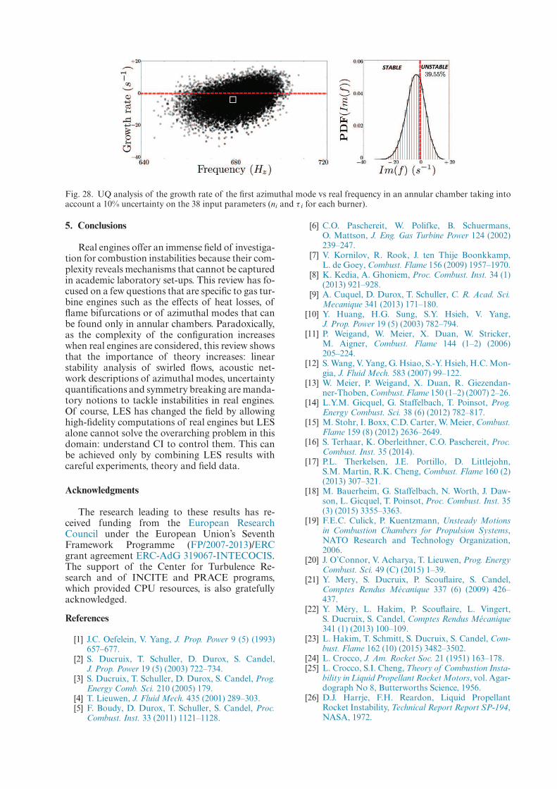
Fig. 28. UQ analysis of the growth rate of the rst azimuthal mode vs real frequency in an annular chamber taking into account a 10% uncertainty on the 38 input parameters ( n i and τ i for each burner).

5. Conclusions

Real engines offer an immense eld of investiga- tion for combustion instabilities because their com- plexity reveals mechanisms that cannot be captured in academic laboratory set-ups. This review has fo- cused on a few questions that are speci c to gas tur- bine engines such as the effects of heat losses, of "ame bifurcations or of azimuthal modes that can be found only in annular chambers. Paradoxically, as the complexity of the con guration increases when real engines are considered, this review shows that the importance of theory increases: linear stability analysis of swirled "ows, acoustic net- work descriptions of azimuthal modes, uncertainty quanti cations and symmetry breaking are manda- tory notions to tackle instabilities in real engines. Of course, LES has changed the eld by allowing high- delity computations of real engines but LES alone cannot solve the overarching problem in this domain: understand CI to control them. This can be achieved only by combining LES results with careful experiments, theory and eld data.

Acknowledgments

The research leading to these results has re- ceived funding from the European Research Council under the European Union’s Seventh Framework Programme ( FP/2007-2013 )/ ERC

grant agreement ERC-AdG 319067-INTECOCIS . The support of the Center for Turbulence Re- search and of INCITE and PRACE programs, which provided CPU resources, is also gratefully acknowledged.

References

[1] J.C. Oefelein , V. Yang , J. Prop. Power 9 (5) (1993) 657–677 .

[2] S. Ducruix , T. Schuller , D. Durox , S. Candel , J. Prop. Power 19 (5) (2003) 722–734 .

[3] S. Ducruix , T. Schuller , D. Durox , S. Candel , Prog. Energy Comb. Sci. 210 (2005) 179 .

[4] T. Lieuwen , J. Fluid Mech. 435 (2001) 289–303 . [5] F. Boudy , D. Durox , T. Schuller , S. Candel , Proc.

Combust. Inst. 33 (2011) 1121–1128 .

[6] C.O. Paschereit , W. Polifke , B. Schuermans , O. Mattson , J. Eng. Gas Turbine Power 124 (2002) 239–247 .

[7] V. Kornilov , R. Rook , J. ten Thije Boonkkamp , L. de Goey , Combust. Flame 156 (2009) 1957–1970 .

[8] K. Kedia , A. Ghoniem , Proc. Combust. Inst. 34 (1) (2013) 921–928 .

[9] A. Cuquel , D. Durox , T. Schuller , C. R. Acad. Sci. Mecanique 341 (2013) 171–180 .

[10] Y. Huang , H.G. Sung , S.Y. Hsieh , V. Yang , J. Prop. Power 19 (5) (2003) 782–794 .

[11] P. Weigand , W. Meier , X. Duan , W. Stricker , M. Aigner , Combust. Flame 144 (1–2) (2006) 205–224 .

[12] S. Wang , V. Yang , G. Hsiao , S.-Y. Hsieh , H.C. Mon- gia , J. Fluid Mech. 583 (2007) 99–122 .

[13] W. Meier , P. Weigand , X. Duan , R. Giezendan- ner-Thoben , Combust. Flame 150 (1–2) (2007) 2–26 .

[14] L.Y.M. Gicquel , G. Staffelbach , T. Poinsot , Prog. Energy Combust. Sci. 38 (6) (2012) 782–817 .

[15] M. Stohr , I. Boxx , C.D. Carter , W. Meier , Combust. Flame 159 (8) (2012) 2636–2649 .

[16] S. Terhaar , K. Oberleithner , C.O. Paschereit , Proc. Combust. Inst. 35 (2014) .

[17] P.L. Therkelsen , J.E. Portillo , D. Littlejohn , S.M. Martin , R.K. Cheng , Combust. Flame 160 (2) (2013) 307–321 .

[18] M. Bauerheim , G. Staffelbach , N. Worth , J. Daw- son , L. Gicquel , T. Poinsot , Proc. Combust. Inst. 35 (3) (2015) 3355–3363 .

[19] F.E.C. Culick , P. Kuentzmann , Unsteady Motions in Combustion Chambers for Propulsion Systems , NATO Research and Technology Organization, 2006 .

[20] J. O’Connor , V. Acharya , T. Lieuwen , Prog. Energy Combust. Sci. 49 (C) (2015) 1–39 .

[21] Y. Mery , S. Ducruix , P. Scou"aire , S. Candel , Comptes Rendus Mécanique 337 (6) (2009) 426–437 .

[22] Y. Méry , L. Hakim , P. Scou"aire , L. Vingert , S. Ducruix , S. Candel , Comptes Rendus Mécanique 341 (1) (2013) 100–109 .

[23] L. Hakim , T. Schmitt , S. Ducruix , S. Candel , Com- bust. Flame 162 (10) (2015) 3482–3502 .

[24] L. Crocco , J. Am. Rocket Soc. 21 (1951) 163–178 . [25] L. Crocco , S.I. Cheng , Theory of Combustion Insta-

bility in Liquid Propellant Rocket Motors , vol. Agar- dograph No 8, Butterworths Science, 1956 .

[26] D.J. Harrje , F.H. Reardon , Liquid Propellant Rocket Instability, Technical Report Report SP-194 , NASA, 1972 .

[27] S. Hochgreb , D.J.C. Dennis , I. Ayranci , W. Bain- bridge , S. Cant , in: Proceedings of ASME Turbo Expo 2013—GT2013-9531, 2013 .

[28] M.d.l.C. García , E. Mastorakos , A.P. Dowling , Combust. Flame 156 (2) (2009) 374–384 .

[29] J. Kopitz , A. Huber , T. Sattelmayer , W. Polifke , in: ASME GT2005-68797, Reno, NV, U.S.A., 2005 .

[30] N. Worth , J. Dawson , Proc. Combust. Inst. 34 (2012) 1–8 .

[31] J.F. Bourgouin , D. Durox , J.P. Moeck , T. Schuller , S. Candel , Proc. Combust. Inst. 35 (3) (2015) 3237–3244 .

[32] W. Krebs , G. Walz , S. Hoffmann , in: 5th AIAA

Aeroacoustics Conference AIAA 99-1971, 1999 . [33] P. Berenbrink , S. Hoffmann , in: ASME Turbo Expo

2001. Paper 2001-GT-42, 2001 . [34] W. Krebs , P. Flohr , B. Prade , S. Hoffmann , Com-

bust. Sci. Technol. 174 (2002) 99–128 . [35] S. Candel , Proc. Combust. Inst. 29 (1) (2002) 1–28 . [36] T. Lieuwen , V. Yang , Combustion Instabilities

in Gas Turbine Engines. Operational Experience, Fundamental Mechanisms and Modeling, Prog. in Astronautics and Aeronautics AIAA, vol. 210, 2005 .

[37] L.P.H. De Goey , J.A. van Oijen , V.N. Kornilov , J.H.M. ten Thije Boonkkamp , Proc. Combust. Inst. 33 (1) (2011) 863–886 .

[38] T. Poinsot , A. Trouvé, D. Veynante , S. Candel , E. Esposito , J. Fluid Mech. 177 (1987) 265–292 .

[39] M. Ihme , H. Pitsch , H. Bodony , Proc. Combust. Inst. 32 (2009) 1545–1554 .

[40] S. Candel , D. Durox , S. Ducruix , A. Birbaud , N. Noiray , T. Schuller , Int. J. Acoust. 8 (2009) 1–56 .

[41] L. Rayleigh , Nature July 18 (1878) 319–321 . [42] A.A. Putnam , J.M. Beer , Combustion Driven Oscil-

lations in Industry, Fuel and Energy Science Series, American Elsevier, 1971 .

[43] F.A. Williams , Combustion Theory , Benjamin Cum- mings, Menlo Park, CA, 1985 .

[44] E.W. Price , in: 12th Symp. (Int.) on Combus- tion, The Combustion Institute, Pittsburgh, 1969, pp. 101–113 .

[45] M. Barrère , F.A. Williams , Proc. Combust. Inst. 12 (1968) 169–181 .

[46] W. Strahle , Prog. Energy Combust. Sci. 4 (1978) 157–176 .

[47] B.D. Mugridge , J. Sound Vib. 70 (1980) 437–452 . [48] V. Yang , F.E.C. Culick , Combust. Sci. Technol. 45

(1986) 1–25 . [49] D.G. Crighton , A.P. Dowling , J.E.F. Williams ,

M. Heckl , F. Leppington , Modern Methods in An- alytical Acoustics, Lecture Notes, Springer Verlag, New-York, 1992 .

[50] S. Candel , C. Huynh. , T. Poinsot , in: NATO ASI Se- ries, Kluwer Academic Publishers, Dordrecht, 1996, pp. 83–112 .

[51] A.P. Dowling , J. Sound Vib. 180 (4) (1995) 557–581 . [52] C. Martin , L. Benoit , Y. Sommerer , F. Nicoud ,

T. Poinsot , AIAA J. 44 (4) (2006) 741–750 . [53] A.S. Morgans , S.R. Stow , Combust. Flame 150 (4)

(2007) 380–399 . [54] P.L. Rijke , Phil. Mag. 17 (1859a) 419–422 . [55] P.L. Rijke , Ann. Phys. 107 (1859b) 339 . [56] J. Moeck , M. Oevermann , R. Klein , C. Paschereit ,

H. Schmidt , Proc. Combust. Inst. 32 (2009) 1199–1207 .

[57] J. Moeck , M. Paul , C. Paschereit , in: ASME Turbo Expo 2010 GT2010-23577, 2010 .

[58] E. Courtine , L. Selle , T. Poinsot , Combust. Flame 162 (2015) 4331–4341 .

[59] T. Poinsot , D. Veynante , Theoretical and Numerical Combustion , third ed., 2011 . www.cerfacs.fr/elearning

[60] M. Bauerheim , F. Nicoud , T. Poinsot , Combust. Flame 162 (1) (2015) 60–67 .

[61] K. Truf n , T. Poinsot , Combust. Flame 142 (4) (2005) 388–400 .

[62] T. Sayadi , P.J. Schmid , F. Richecoeur , D. Durox , Phys. Fluids 27 (3) (2015) 037102 .

[63] N. Noiray , D. Durox , T. Schuller , S. Candel , J. Fluid Mech. 615 (2008) 139–167 .

[64] D. Durox , T. Schuller , N. Noiray , S. Candel , Proc. Combust. Inst. 32 (1) (2009) 1391–1398 .

[65] P. Palies , D. Durox , T. Schuller , S. Candel , Combust. Flame 158 (10) (2011) 1980–1991 .

[66] T. Lieuwen , B.T. Zinn , Proc. Combust. Inst. 27 (1998) 1809–1816 .

[67] T. Sattelmayer , J. Eng. Gas Turbine Power 125 (2003) 11–19 .

[68] A. Birbaud , S. Ducruix , D. Durox , S. Candel , Com- bust. Flame 154 (3) (2008) 356–367 .

[69] S. Camporeale , B. Fortunato , G. Campa , J. Eng. Gas Turbine Power 133 (1) (2011) .

[70] F. Nicoud , L. Benoit , C. Sensiau , T. Poinsot , AIAA

J. 45 (2007) 426–441 . [71] C. Pankiewitz , T. Sattelmayer , J. Eng. Gas Turbine

Power 125 (3) (2003) 677–685 . [72] A.P. Dowling , S.R. Stow , J. Prop. Power 19 (5)

(2003) 751–764 . [73] K. Kedia , H. Altay , A. Ghoniem , Proc. Combust.

Inst. 33 (2011) 1113–1120 . [74] S. Ducruix , D. Durox , S. Candel , Proc. Combust.

Inst. 28 (1) (2000) 765–773 . [75] P. Schmitt , T. Poinsot , B. Schuermans , K.P. Geigle ,

J. Fluid Mech. 570 (2007) 17–46 . [76] C. Fureby , Flow Turbine Combust. 84 (2010)

543–564 . [77] N. Noiray , M. Bothien , B. Schuermans , Combust.

Theory Model. 15 (2011) 585–606 . [78] G. Bloxsidge , A. Dowling , N. Hooper ,

P. Langhorne , AIAA J. 26 (1988) 783–790 . [79] T. Poinsot , W. Lang , F. Bourienne , S. Candel , E. Es-

posito , J. Prop. Power 5 (1989) 14–20 . [80] G. Billoud , M. Galland , C. Huynh , S. Candel , Com-

bust. Sci. Technol. 81 (1992) 257–283 . [81] J. Seume , N. Vortmeyer , W. Krause , J. Hermann ,

C. Hantschk , P. Zangle , S. Gleis , D. Vortmeyer , A. Orthmann , J. Eng. Gas Turbines Power 120 (1998) 721–726 .

[82] N. Gourdain , L. Gicquel , M. Montagnac , O. Ver- morel , M. Gazaix , G. Staffelbach , M. Garcia , J. Boussuge , T. Poinsot , Comput. Sci. Discovery 2 (2009a) 015003 .

[83] N. Gourdain , L. Gicquel , G. Staffelbach , O. Ver- morel , F. Duchaine , J.-F. Boussuge , T. Poinsot , Comput. Sci. Discovery 2 (1) (2009b) 28pp .

[84] G. Staffelbach , L. Gicquel , G. Boudier , T. Poinsot , Proc. Combust. Inst. 32 (2009) 2909–2916 .

[85] P. Wolf, G. Staffelbach , L. Gicquel , J.-D. Muller , T. Poinsot , Combust. Flame 159 (11) (2012) 3398–3413 .

[86] J. Bourgouin , D. Durox , J.P. Moeck , T. Schuller , S. Candel , in: ASME Turbo Expo 2013 GT2013-95010, 2013 .

[87] N. Worth , J. Dawson , in: Proc. Combust. Inst., vol. 34, 2013, pp. 3127–3134 .

[88] N. Noiray , B. Schuermans , Proc. R. Soc. A: Math. Phys. Eng. Sci. 469 (2151) (2012) 20120535 .

[89] B. Schuermans , C. Paschereit , P. Monkewitz , in: 44th AIAA Aerospace Sciences Meeting and Ex- hibit, vol. AIAA paper 2006-0549, 2006 .

[90] C. Sensiau , F. Nicoud , T. Poinsot , Int. J. Aeroacoust. 8 (1) (2009) 57–68 .

[91] G. Ghirardo , M. Juniper , in: 2013-0232, 2013 . [92] N. Worth , J. Dawson , Combust. Flame 160 (11)

(2013) 2476–2489 . [93] J.-F. Bourgouin , D. Durox , J.P. Moeck , T. Schuller ,

S. Candel , J. Eng. Gas Turbine Power 137 (2) (2015) 021503-11 .

[94] F. Baillot , F. Lespinasse , Combust. Flame 161 (5) (2014) 1247–1267 .

[95] J. O’Connor , T. Lieuwen , J. Eng. Gas Turbine Power 134 (011501-9) (2012) 134 .

[96] J. Blimbaum , M. Zanchetta , T. Akin , V. Acharya , J. O’Connor , D. Noble , T. Lieuwen , Int. J. Spray Combust. Dyn. 4 (4) (2012) 275–298 .

[97] V. Acharya , M. Malanoski , M. Aguilar , T. Lieuwen , J. Eng. Gas Turbine Power 136 (5) (2014) 051503-10 .

[98] F. Lespinasse , F. Baillot , T. Boushaki , C. R. Acad. Sci. Mec. 341 (1–2) (2013) 110–120 .

[99] J.-F. Parmentier , P. Salas , P. Wolf, G. Staffelbach , F. Nicoud , T. Poinsot , Combust. Flame 159 (7) (2012) 2374–2387 .

[100] S. Evesque , W. Polifke , C. Pankiewitz , in: 9th AIAA/CEAS Aeroacoustics Conference, vol. AIAA Paper 2003–3182, 2003 .

[101] M. Bauerheim , J.-F. Parmentier , P. Salas , F. Nicoud , T. Poinsot , Combust. Flame 161 (5) (2014) 1374–1389 .

[102] L. Li , X. Sun , Combust. Flame 162 (3) (2015) 628–641 .

[103] M. Bauerheim, P. Salas, F. Nicoud, T. Poinsot, J. Fluid Mech. 760 (2014) 431–465, doi: 10.1017/jfm. 2014.578 .

[104] A. Davey , H. Salwen , J. Fluid Mech. 281 (1994) 357–369 .

[105] J. Guckenheimer , A. Mahalov , Phys. Rev. Lett. 68 (1992) 2257 .

[106] A. Sengissen , J.F.V. Kampen , R. Huls , G. Stoffels , J.B.W. Kok , T. Poinsot , Combust. Flame 150 (2007) 40–53 .

[107] R. Garby , L. Selle , T. Poinsot , C. R. Acad. Sci. Mec. 341 (1–2) (2013) 220–229 .

[108] K. Kedia , A. Ghoniem , Combust. Flame 162 (4) (2015) 1304–1315 .

[109] R. Raun , M. Beckstead , Combust. Flame 94 (1993) 1–24 .

[110] K.J. Bosschaart , L. de Goey , Combust. Flame 132 (1–2) (2003) 170–180 .

[111] K.J. Bosschaart , L.P.H. De Goey , Combust. Flame 136 (3) (2004) 261–269 .

[112] F. Duchaine , F. Boudy , D. Durox , T. Poinsot , Com- bust. Flame 158 (12) (2011) 2384–2394 .

[113] D. Mejia , L. Selle , R. Bazile , T. Poinsot , Proc. Com- bust. Inst. 35 (3201–3208) (2014) 3 .

[114] L. Boyer , J. Quinard , Combust. Flame 82 (1990) 51–65 .

[115] M. Flei l , A.M. Annaswamy , Z.A. Ghoneim , A.F. Ghoniem , Combust. Flame 106 (4) (1996) 487–510 .

[116] S.H. Lee , J.G. Ih , K.S. Peat , J. Sound Vib. 303 (3–5) (2007) 741–752 .

[117] R. Rook , L. de Goey , L. Somers , K. Schreel , R. Parchen , Combust. Theory Model. 6 (2) (2002) 223–242 .

[118] M. Hoeijmakers , V. Kornilov , I.L. Arteaga , P. de Goey , H. Nijmeijer , Combust. Flame 161 (2014) 2860–2867 .

[119] T. Emmert , S. Bomberg , W. Polifke , Combust. Flame 162 (1) (2015) 75–85 .

[120] E. Courtine , L. Selle , F. Nicoud , W. Polifke , C.F. Silva , M. Bauerheim , T. Poinsot. , in: Proc. of the Summer Program, Center of Turbulence Re- search, Stanford University/NASA, Ames, USA, 2014, pp. 169–178 .

[121] F. Hussain , J. Jeong , J. Fluid Mech. 285 (1995) 69–94 .

[122] A.L. Birbaud , D. Durox , S. Ducruix , S. Candel , Phys. Fluids 19 (2007) 013602 .

[123] E. Motheau , L. Selle , F. Nicoud , J. Sound Vib. 333 (1) (2013) 246–262 .

[124] E. Motheau , F. Nicoud , T. Poinsot , J. Fluid Mech. 749 (2014) 542–576 .

[125] F.E. Marble , S. Candel , J. Sound Vib. 55 (1977) 225–243 .

[126] M. Huet , A. Giauque , J. Fluid Mech. 733 (2013) 268–301 .

[127] I. Duran, S. Moreau, J. Fluid Mech. 723 (2013) 190–231, doi: 10.1017/jfm.2013.118 .

[128] W. Lang , T. Poinsot , S. Candel , Combust. Flame 70 (1987) 281–289 .

[129] K. McManus , T. Poinsot , S. Candel , Prog. Energy Combust. Sci. 19 (1993) 1–29 .

[130] N. Tran , S. Ducruix , T. Schuller , Proc. Combust. Inst. 32 (2) (2009) 2917–2924 .

[131] B. Cosic , B. Bobusch , J. Moeck , C. Paschereit , J. Eng. Gas Turbine Power 134 (2012) 061502-1 .

[132] W.C. Strahle , J. Fluid Mech. 49 (1971) 399–414 . [133] A.P. Dowling , Y. Mahmoudi , Proc. Combust. Inst.

35 (1) (2015) 65–100 . [134] N.A. Cumpsty , F.E. Marble , Proc. R. Soc. Lond. A

357 (1977) 323–344 . [135] F. Bake , N. Kings , A. Fischer , R. I. , Int. J. Aeroa-

coust. 8 (1–2) (2008) 125–142 . [136] F. Bake , C. Richter , B. Muhlbauer , N. Kings ,

I. Rohle , F. Thiele , B. Noll , J. Sound Vib. 326 (2009) 574–598 .

[137] M. Leyko , F. Nicoud , T. Poinsot , AIAA J. 47 (11) (2009) 2709–2716 .

[138] I. Duran , S. Moreau , T. Poinsot , AIAA J. 51 (1) (2013) 42–52 .

[139] M.S. Howe , J. Fluid Mech. 659 (2010) 267–288 . [140] W. Ullrich , T. Sattelmayer , in: 21st AIAA CEAS

Aeroacoustics Conference, 2015, pp. 1–19 . [141] F.E. Marble , S. Candel , J. Sound Vib. 55 (1977)

225–243 . [142] S. Candel , D. Durox , T. Schuller , J.-F. Bourgouin ,

J.P. Moeck , Ann. Rev. Fluid Mech. 46 (1) (2014) 147–173 .

[143] I. Duran , M. Leyko , S. Moreau , F. Nicoud , T. Poinsot , C. R. Acad. Sci. Mec. 341 (1–2) (2013) 131–140 .

[144] M. Leyko , I. Duran , S. Moreau , F. Nicoud , T. Poinsot , J. Sound Vib. 333 (23) (2014) 6090–6106 .

[145] J. Eckstein , E. Freitag , C. Hirsch , T. Sattelmayer , J. Eng. Gas Turbine Power 128 (2) (2006) 264–270 .

[146] W. Polifke , C. Paschereit , K. Döbbeling , Int. J. Acoust. Vib. 6 (3) (2001) 135–146 .

[147] C.S. Goh , A.S. Morgans , Combust. Sci. Technol. 185 (2) (2013) 249–268 .

[148] A.S. Morgans, C.S. Goh, J.A. Dahan, J. Fluid Mech. 733 (R2) (2013), doi: 10.1017/jfm.2013.448 .

[149] B. Emerson , J. O’Connor , M. Juniper , T. Lieuwen , J. Fluid Mech. 706 (2012) 219–250 .

[150] M. Juniper , J. Fluid Mech. 565 (2006) 171–195 . [151] A. Steinberg , I. Boxx , M. Stöhr , C. Carter ,

W. Meier , Combust. Flame 157 (2010) 2250–2266 . [152] S. Terhaar , K. Oberleithner , C.O. Paschereit , Com-

bust. Sci. Technol. 186 (7) (2014) . [153] K. Oberleithner , M. Stöhr , S.H. Im , C.M. Arndt ,

A.M. Steinberg , Combust. Flame 162 (8) (2015) 3100–3114 .

[154] S. Roux , G. Lartigue , T. Poinsot , U. Meier , C. Bérat , Combust. Flame 141 (2005) 40–54 .

[155] A. Ghani, T. Poinsot, L. Gicquel, J.-D. Muller, Flow, Turbine Combust. 96 (2016) 207–226, doi: 10. 1007/s10494- 015- 9654- 9 .

[156] K. Oberleithner , S. Schimek , C.O. Paschereit , Com- bust. Flame 162 (1) (2015) 86–99 .

[157] J.O. Keller , L. Vaneveld , D. Korschelt , G.L. Hub- bard , A.F. Ghoniem , J.W. Daily , A.K. Oppenheim , AIAA J. 20 (1981) 254–262 .

[158] Y. Sommerer , D. Galley , T. Poinsot , S. Ducruix , F. Lacas , D. Veynante , J. Turbine 5 (2004) 037 .

[159] I. Chterev , C.W. Foley , D. Foti , S. Kostka , A.W. Caswell , N. Jiang , A. Lynch , D.R. Noble , S. Menon , J.M. Seitzman , T.C. Lieuwen , Combust. Sci. Technol. 186 (8) (2014) 1041–1074 .

[160] M.J. Tummers , A.W. Hübner , E.H.v. Veen , K. Han- jali ́c , T.H.v.d. Meer , Combust. Flame 156 (2) (2009) 447–459 .

[161] Y. Huang , V. Yang , Combust. Flame 136 (2004) 383–389 .

[162] Y. Huang , V. Yang , Prog. Energy Combust Sci. 35 (4) (2009) 293–364 .

[163] S. Seo , Parametric Study of Lean Premixed Com- bustion Instability in a Pressurized Model Gas Tur- bine Combustor , Department of Mechanical Engi- neering, Pennsylvania State University, 1999 (Ph.D. thesis) .

[164] S. Hermeth , G. Staffelbach , L.Y. Gicquel , V. Anisi- mov , C. Cirigliano , T. Poinsot , Combust. Flame 161 (1) (2014) 184–196 .

[165] M. Vanierschot , E.V. den Bulck , Exp. Thermal Fluid Sci. 31 (6) (2007) 513–524 .

[166] M. Falese , L.Y. Gicquel , T. Poinsot , Comput. Fluids 89 (2014) 167–178 .

[167] M. Bauerheim , A. Ndiaye , P. Constantine , G. Iac- carino , S. Moreau , F. Nicoud , in: Proceedings of the CTR Summer Program, 2014, pp. 209–210 .

[168] T. Chantrasmi , G. Iaccarino , Int. J. Uncertainty Quantif. 2 (2) (2012) 125–143 .