International Journal of Smart Electrical Engineering, Vol.1, No.3, Fall 2012 ISSN: 2251-9246

181

Predicting the Next State of Traffic by Data Mining

Classification Techniques

S.Mehdi Hashemi1, Mehrdad Almasi

2, Roozbeh Ebrazi

3, Mohsen Jahanshahi

4

1 Department of Mathematical and Computer Science, Amirkabir University of Technology, Tehran, Iran. Email: hashemi@aut.ac.ir 2 Department of Computer Engineering, Isfahan University of Technology, Isfahan, Iran. Email: m.almasi@ec.iut.ac.ir

3 Department of Mathematical and Computer Science, Amirkabir University of Technology, Tehran, Iran. Email: r.ebrazi@aut.ac.ir 4 Young Researchers and Elite club, Central Tehran Branch, Islamic Azad University, Tehran, Iran. Email: mjahanshahi@iauctb.ac.ir

Abstract

Traffic prediction systems can play an essential role in intelligent transportation systems (ITS). Prediction and patterns

comprehensibility of traffic characteristic parameters such as average speed, flow, and travel time could be beneficiary both

in advanced traveler information systems (ATIS) and in ITS traffic control systems. However, due to their complex nonlinear

patterns, these systems are burdensome. In this paper, we have applied some supervised data mining techniques (i.e.

Classification Tree, Random Forest, Naïve Bayesian and CN2) to predict the next state of Traffic by a categorical traffic

variable (level of service (LOS)) in different short-time intervals and also produce simple and easy handling if-then rules to

reveal road facility characteristic. The analytical results show prediction accuracy of 80% on average by using methods.

Keywords: Traffic prediction, Level of Service Prediction, Data Mining, Naïve Bayesian, Random forest, Classification tree, CN2

© 2012 IAUCTB-IJSEE Science. All rights reserved

1. Introduction

Traffic state prediction has an important role in

intelligent transportation systems (ITS). It can be

classified into short-term prediction which predict

traffic state changes in short periods (e.g. 15 min or

30 min) and long-term prediction for monthly or

yearly traffic state information [1]. Short-term

predictions either may be used directly by traffic

experts to take relevant actions or could be injected

as inputs to proactive congestion management

approaches. These approaches could include route

guidance, dynamic congestion pricing, variable speed

limit systems. The long-term predictions can be used

for transportation planning. Although traffic

prediction method studies usually use a measure of

algorithm performance based only on predictive

accuracy, it is accepted by many researchers and

practitioners that, in many application domains, the

comprehensibility of the knowledge (or patterns)

discovered by an algorithm is another important

evaluation criterion. For example, the pattern

discovered by this algorithm is used to support a

decision that will be made by a human user, rather

than for automated decision-making. Therefore, an

ideal method is one that covers both application

aspects.

Lili et al [28] specify three factors that affect

the quality of the predicted real-time traffic

information. These factors include: (1) Variability in

the quality of real-time data from different sources

(sensors or other road facilities). (2) Dynamic nature

of real-time traffic conditions, which cause delay

between the time data, is collected and is used. (3)

Randomness and stochastic inherent of traffic

networks which appear in supply, demand, and

performance of the traffic network. For these

reasons, they conclude that predicting short-term

traffic conditions is more meaningful.

Besides short-term and long-term predictions

classes, there exist various classification standards

that categorize traffic prediction methods such as

pp.181:193

International Journal of Smart Electrical Engineering, Vol.1, No.3, Fall 2012 ISSN: 2251-9246

182

single link or transportation network, freeways or

urban streets, univariate or multivariate, physical

models or mathematical methodologies, etc [49].

Applying statistical methodology, prediction

methods are divided into two main categories:

(1) Parametric method which includes linear and

nonlinear regression ([48], [45], [44]) filtering

techniques ([43], [46) autoregressive moving average

family (ARMA/ARIMA/SARIMA) [32]. These

techniques try to detect a function between the past

information and the predicted state. However, they

are typically sensitive to errors and data quality.

(2) Non-parametric method such as Neural Networks

(Feed-Forward Neural Network (FFNN) [50], Radial

Basis Function Neural Networks (RBF-NN) ([34],

etc.), Bayesian networks [20], K-Nearest Neighbor

(KNN) Algorithms [41], Support Vector Regression

(SVR) ([10], [24]). This kind of techniques can

generally handle imprecise data and as a result,

usually perform well in treating the nondeterministic,

complex and nonlinear systems.

Up to now, several approaches (usually by

utilizing unsupervised algorithms) consider

prediction of continuous traffic parameters: flow,

travel time, etc. ([13], [28], [12], [41]). In this paper,

we predict short-term level of service (LOS) of a

highway section by using supervised learning

algorithms and also propose representations of

classification models in terms of if-then rule sets

which can give the comprehensibility of the

knowledge (or patterns) discovered by a

classification algorithm. In following, we describe

some motivations for prediction of this traffic state

categorical variable:

Traffic patterns and driver behavior in different

times and traffic states (e.g. free-flow, stable or

synchronized flow, congested flow and flow near to

jam density) is quite different [9]. This phenomena

cause some problem for traffic simulation models to

capture characteristics of traffic flow. For example

analytical functions that is used to describe the

relationship between flow and density (fundamental

diagram) fails to satisfy all of the desirable properties

so that the traffic simulation models that use these

functions as input model parameters will deteriorate

and only make a reasonable prediction in relatively

short time scale [27]. One of the key applications of

categorically traffic state prediction can be setting

specific boundary conditions and calibration

parameters for simulation models, or fitting separate

functions (to describe fundamental diagrams) for

each LOS, and then using them according to the

predicted LOS in advance. This method can increase

accuracy of macroscopic simulation models which

has broad usage in ITS proactive controller ([33],

[22], [19]).

Classification prediction methods which have

been used in this study for prediction, also produce

simple and easy handling if-then rules that can be

used in designing expert systems, scheming decision

tree of a traffic controller system with very light

computation (such as Variable Speed Limit system

[2]). However, in addition to controller system traffic

experts also could mine these simple produced IF-

THEN rules to find performance quality of road,

facility characteristics and propose optimal speed for

that section or detect any failure in the specified

state.

Classification methods such as Naïve Bayesian

can also offer a valuable insight into the structure of

the training data and effects of each attributes of

traffic state and providing traffic engineers with a

comprehensible explaining the system’s predictions.

Which guide them by interpretation traffic state

occurring, recognition important attribute and

reasons for and using this information to off line

network planning. The rest of the paper is organized as follows:

Section 2 describes the model-learning framework,

brief description of each classification learner and

setting parameters and heuristic, which is used in the

learning process. Section 3 presents the results and

discusses the experiments performed and finally the

conclusion is presented in section 4.

2. Proposed Approach

Data mining proposes varieties knowledge

discovery methods. These methods include

classification and prediction, and presenting the

mining results using visualization tools. The term

prediction denotes to both numeric prediction and

class label prediction.

In particular, a classification problem aims to

generate (to learn) a model, called classifiers, which

is able to predict the value of a categorical target

variable (class labels) based on several input

variables (sometimes called predictor variables,

fields, attributes or features). This model actually is a

function that maps an input attribute vector X from

attributes space to output class label

{ }. Before learning the model, the

class labels and the values of the attributes for each

record (observation, instance or example) must be

known. Data in a labeled training set comes in

records of the form:

( ) (( ) ) (1)

The dependent variable (class labels) Y is the

target variable that we are trying to predict

(understand, classify or generalize) and the

International Journal of Smart Electrical Engineering, Vol.1, No.3, Fall 2012 ISSN: 2251-9246

183

vector X is composed of the attributes 1x , 2x , 3x ,…,

nx .

In this study, we have tested four famous data

mining classification algorithm, i.e. Classification

tree, Random Forest, Naïve Bayesian and CN2,

which are widely utilized in artificial intelligence. In

addition to this method, we tested support vector

machine for prediction but it did not show good

enough accuracy so we left it out from our study, this

result match with previous Chen and et al [12] study.

In our application, first, the reliable data are

gathered, then the days with missing or error record

was omitted after that, traffic parameters of each time

interval extracted from data. We learn the predictive

model of extracted training set comes in the records

include Flow (veh/15 min), Density (veh/km), Speed

(km/h), Time Duration (start time of interval in min)

as the attributes for different time intervals (of 10,

15, and 30 minutes). LOS of the next time interval is

considered as class label or the target variable of it.

For example the record form of time interval one

(t=1) is in the form of (2).

( ) (2)

In fact, this prediction framework is

independence of current traffic’s state. The keynote

has laid down on learning offline prediction models

with traffic’s history data and using it to preform

prediction based on classification current data. This

ability makes it robust to handle given noisy data or

data with missing values.

The reminder of this Section will present a brief

description of well-known classification methods,

their logical sequence of the prediction method and

specific modification of them that we have used in

this paper.

2.1. Classification Tree

Decision Tree is a convenient, nonparametric

and widely used learning approach in data mining as

a classifier. Classification and Regression tree [7] are

two main types of Decision trees. Classification tree

used when the value of predicted item is a class and

Regression tree is utilized when predicted item have

a real number.

Decision Tree is a directed rooted tree of nodes

and connecting branches. Nodes indicate decision

points, chance events, or branch terminals, which

correspond to one of the input variables. Branches

correspond to each possible value of that input

variable or event outcome emerging from a node.

Each leaf represents a value of the target variable.

When Decision Tree receives a new data, a passing

through nodes of it, determine the next state of traffic

and will give new instance’s target variable. Each

path from the root of a decision tree to one of its

leaves results a rule.

This tree model is usually learned top-down by

recursively partitioning [16] the instance space (The

set of all possible observations which equals to the

training set in learning phase). At each node, a

predictor variable select to split the set so that the

created partitions have similar target variable value.

The selection criteria for choosing variable defined

as how homogeneous the resulted partitions are.

Different algorithms use various selection criteria

e.g., Gini index [7], Information Gain [36],

Likelihood-Ratio Chi Squared Statistics [4], etc.

These selection criteria can be grouped according to

the source of them such as information theory,

dependence, and distance [5] or according to the

measure structure: impurity based criteria,

normalized impurity based criteria and binary criteria

[39]. This process continues until no partitions gain a

sufficient splitting criterion measure or meets one or

more stopping criteria. For example, all cases put

into a similar target variable partition or the tree

reaches the specified maximum depth. This phase of

learning the decision tree called Growing phase.

Exploiting loosely stopping criteria tends to generate

large decision trees. To handle this situation some

algorithm utilized pruning phase suggested in [7].

This phase transforms large decision trees to smaller

one by cutting some sub-branches that absent of

them does not make big accuracy change and the tree

model keep its sufficient generalization exactness.

Algorithms that generate a decision are called

decision tree inducers. Various decision trees

inducers exist such as ID3 [35], C4.5 [37], CART

[7], CHAID [25], QUEST [29].

In our application, we select Information Gain,

which will be explained in following subsection, in

the role of selection criterion for the learner. Pruning

during induction is based on the minimal number of

two instances in leaves i.e. the algorithm does not

construct a split, which would put less than two of

training examples in any of the branches. Since target

variable (LOS) value is a class then the resulted

decision tree is a classification tree (Fig.2).

2.1.1. Information Gain

This measure is based on information theory,

which indicates required information to classify a

given record of data. The expected information to

encode possible class label Y of an arbitrary record

of a training set in bits is given by (3).

( ) ∑ ( ) ( ( )) (3)

Where ( ) is the nonzero probability

that the record belongs to a class . A log function

to the base two is used, because the information is

International Journal of Smart Electrical Engineering, Vol.1, No.3, Fall 2012 ISSN: 2251-9246

184

encoded in bits. ( ) is also known as the entropy

of the data. This parameter gets a high value if class

label Y has uniform distribution in training set and

low value if its distribution varies. The conditional

entropy ( ) is the expected information

required to classify a record based on some known

attribute ax :

( ) ∑ ( ) ( ) ( ) (4)

Information gain is defined as the difference

between the original information requirement (3) and

the new requirement after obtaining the value of

(4). That is

( ) ( ) ( ) (5)

In other words, ( ) reveal how much

information would be gained by splitting on . We

like to do splitting on the attribute that would

produce partitions that are more pure and the amount

of information still required to finish classifying their

records is minimal. Therefore, it is sufficient to

choose the attribute with the highest information gain

and using it as a splitting attribute on the current

node in Decision Tree.

Fig.2. A portion of the resulted classification tree, the color of the

node report on the probability of the majority class (Majority class probability) that the color intensity would be higher towards the

leaves of the node

2.2. Random Forest

Random forest method, proposed firstly by Leo

Brieman [8], builds ensemble or committee of

decision trees (classification or regression trees) with

given the set of class-labeled data and aggregate

results of them for prediction. For inducing each

individual tree, the algorithm utilizes bagging idea

[6] and the random selection [17] of features,

introduced independently by Ho [23] and Amit and

Geman [3].

Similar to bagging, the algorithm grows each

individual tree from a bootstrap sample (with the

same size, drawn randomly with replacement) or a

subsample (with smaller size, drawn randomly

without replacement) of the training data. Another

technique that Random forest uses to develop trees,

that are even more diverse, is the random variable

selection. It draws an arbitrary subset of variable

from which the best variable is selected for the split.

Originally, Brieman [8] proposed to grow the trees

without any pruning. Its final prediction is the mean

prediction (regression) or class with maximum votes

(classification) of the decision trees.

Let be the number of trees and Mtry the

number of predictor variable drawn at each node. In

case of traffic state application, we set

classification trees to be included in the forest and

Mtry =2 for splitting consideration at each node. As

the stopping condition, minimal number five of

instances in the node before splitting was set.

2.3. Naïve Bayesian

Naïve Bayesian is statistical classifier that

determines class membership probabilities of a given

sample for each class ( ), { }. Naïve Bayesian classifier is based on "naive" class-

conditional independence assumption and Bayes’

theorem. Class-conditional independence implies that

the probability distribution of an attribute value of a

given class is independent of the values of the other

attributes Naïve assumption allows us to estimate

each distribution independently as a one-dimensional

distribution rather than computation-intensive joint

distribution.

( | ) ( ) (6)

According to Bayes’ theorem, the posterior

probability of class conditioned on attribute

vector X expresses in terms of the marginal

(evidence) probability ( ), the prior probability

(probability of hypothesis before seeing any

data X) ( ) and the likelihood probability

(probability of the data X if the hypothesis is

true) ( ) as (7).

( ) ( ) ( )

( ) (7)

The numerator of (7) transforms to the joint

distribution probability ( ) which by n

times applying chain can be described in terms of

conditional probabilities equation (8).

International Journal of Smart Electrical Engineering, Vol.1, No.3, Fall 2012 ISSN: 2251-9246

185

( ) ( ) ( ) ( ) ( ) (8)

And by using Naïve assumption of (6), this equation

expressed as

( ) ( ) ( ) ( ) ( ) ( ) ∏ ( )

(9)

When a new record of attribute values ( ) come, the

classifier predicts the value of Y the class makes

having the highest posterior probability

( ). This is known as the maximum a

posteriori (MAP) decision rule. Therefore, since the

numerator of (7) does not depend on and by

using equation (9) the Naïve Bayesian classifier is a

function which defined as:

( ) ( ( ) ∏ ( ) ) (10)

The parameters of a naive Bayes model i.e. the

class prior probabilities ( ) and the posterior

probability ( ). They can be estimated

from data by maximum-likelihood estimation

(MLE). Given the training data, the class prior

probabilities may be simply estimated by the relative

frequency (number of samples in the class) / (total

number of samples)). To compute ( ) one must assume a distribution or generate

nonparametric models for the attribute. The typical

approach in two following situations is [21]:

1. If xi is categorical then ( ) can be

estimated by the relative frequency.

2. If xi is continuous-valued then it assume that

( ) have Normal (Gaussian distribution),

calculate the mean and standard deviation of

the attribute values xi for training samples in the class

and substitute them into Gaussian distribution

formula (11).

( )

√ (

)

(11)

Depending on the precise nature of the

probability model, naive Bayes classifiers can be

trained very efficiently in a supervised learning

setting. In many practical applications, parameter

estimation for naive Bayes models uses the method

of maximum likelihood; in other words, one can

work with the naive Bayes model without believing

in Bayesian probability or using any Bayesian

methods.

In our traffic state prediction, we also used

Laplace estimator [11] in probability estimation of

prior and conditional probability. It avoids

subsequent problem in the situation when there is no

training sample for the specific class. This situation

would return a zero probability and would cancel the

effects of all the other (posterior) probabilities

involved in the product (9) Laplace estimator

assumes that the training data is so large and simply

add one to each count that is needed to estimate

probabilities.

2.4. CN2

Beside decision tree, a second way to generate

if-then rules is to use rule induction algorithms,

which search for propositional rules directly from the

training data. CN2 [15] is one the most famous

example of this type of approach. It has two main

procedures: On upper level it runs a sequential covering

strategy (also known as separate-and-conquer or

cover-and-remove), first employed by the AQ

Algorithm [30]. This process sequentially extracts

rule from the training set by calling the lower level

procedure (conquer step), and remove data records

that are covered by the rule (separate step). It

continues this routine until no more efficient rules be

discovered. In addition to this exclusive covering

strategy, as in the original CN2 is used [15],

Alternative type of covering is weighted covering,

which only decreases the weight of covered records

instead of removing them[26].

On the lower level, a beam search method is

done. Beam search start with an empty rule (no

conditions on its if-part) and iteratively specialize it,

evaluates the extended rules created by the

specialization operation, and keep the b best-

extended rules (Beam width). This process is

repeated until a stopping criterion is satisfied. In this

process, rule evaluation is done with the aim of

heuristic functions that consider coverage (number of

records covered by a rule) and accuracy during the

process of building a rule. Taking inspiration from

ID3, original CN2 uses entropy (1) as the rule

evaluation function but Clark and Boswell [14]

present the Laplace estimation as an alternative rule

quality measure to overcome undesirable “downward

bias” of entropy and it is defined in Equation (12).

( )

(12)

In the formula (12), P represent the number of

positive examples covered by a rule R in the training

set, n is the number of negative examples covered by

a rule R and k is the number of classes available in

the training set. In addition to these functions there is

many others like m-estimate of probability [18]

and WRACC (weighted CN2-SD algorithmcy), used

in CN2-SD algorithm [26].

In addition to the evaluation function, CN2 uses

a statistical significance test to ensure the new rule

International Journal of Smart Electrical Engineering, Vol.1, No.3, Fall 2012 ISSN: 2251-9246

186

reflects a true correlation between attributes and

classes, and is not due to chance. Actually, it is pre-

pruning method, which avoids generating too

specific rule. It applies the likelihood ratio statistic

test (LRS) to compare the observed class distribution

among examples satisfying the rule with the class

distribution result if the rule had selected examples

randomly. The user determines required significance

level of a rule (i.e. Alpha in LRS test).

The rule models generated by a rule induction

algorithm can be different slightly by changes in

upper level process. Classical CN2 [15] generates

ordered rules (also known as rule lists or decision

lists) in this case the first rule in the ordered list that

covers the new example will classify it. Unordered

CN2 [14] induces unordered rules (rule sets).

Similar to learning in classical CN2, the process of

on the upper level is separated to learn rules for each

class.. In the latter case, all the rules in the model are

used to classify a new example and when more than

one rule covers a new example, and the class

predicted by them is not the same, a tiebreak

criterion is used to decide which rule assess the class

of new example more accurate.

In our implementation, on the upper level we

adopt an exclusive covering, as Unordered CN2 [14].

On the lower level, we used Laplace estimation as

evaluation functions. Pre-pruning of rules is done by

using of two LRS test and indicating minimum rule

coverage threshold. The First LRS test ensures the

minimum required significance level of a rule

when compared to the default rule. In addition, we

use a second LRS test; in this case, the rule is

compared to its parent rule: it verifies whether the

last specialization of the rule has enough significant

level . Finally Minimum coverage threshold

specifies the minimal number of examples that each

induced rule must cover. The value for the setting

parameters are listed in Table.2.

Table.2

The setting parameters of CN2 Time Interval (min)

1 2 Minimum

Coverage

10 0.050 0.020 9

15 0.065 0.020 7

30 0.070 0.020 6

3. Results

To test performance, we used Java

programming language to write required procedures

for extracting traffic parameters and Level of service

with the definition corresponded to the Highway

Capacity Manual [42] form raw data then the

classification model was built through the widget and

python scripting in Orange software. Data for this

study come from real-world traffic data set of Hakim

highway in Tehran, Iran, which has been gathered in

the autumn 2011 with radar traffic sensor. This data

set has been obtained from Tehran Traffic control

Co. that includes 2519011 instances. Processing

these instances, traffic parameters extracted for time

intervals with the length of 10, 15 and 30 minutes

which respectively result in 12358, 8245, 4121

records. Due to lack of records in LOS B and E,

these levels have been merged with their adjacent

ones.

3.1. Model Evaluation

The holdout method was used for model

evaluation (Fig.2). According to this method, the

given data were randomly partitioned into two

independent sets, a training set and a test set. The

records of 14 days of the data are allocated to the

training set, and the remaining is allocated to the test

set In Model Builder part that contains Classification

Tree, Random Forest, Naïve Bayes and CN2 model

inducers, the training set was used to derive the

model. Test Learner and Calculate Accuracy part

uses output models of Model builder part for

prediction of next state of test data and compare it

with the real state of traffic to estimate model’s

accuracy.

Training Data

Test Data

Model Builder

Test Learner&

Calculate Accuraccy

Data

Fig.3. Accuracy estimation with the holdout method

International Journal of Smart Electrical Engineering, Vol.1, No.3, Fall 2012 ISSN: 2251-9246

187

Table.2 provides the model evaluation results

and compare the performance of all the classification

models on the record forms of 10, 15, and 30 minutes

time intervals. In these tables:

Classification accuracy (CA) is the proportion

of correctly classified examples, Sensitivity (Sens)

(also called true positive rate (TPR), hit rate and

recall) is the number of detecting positive examples

among all positive examples, e.g. The proportion of

sick people correctly diagnosed as sick, Brier score

(Brier) measures the accuracy of probability

assessments, which measures the average deviation

between the predicted probabilities of events and the

actual events.

Table.3 Performance comparison of the classification models

Method Time

Interval (min)

CA Sens Brier

Class A Class B Class C Class D

Classification

Tree

10 0.7962 89.50% 84.00% 70.40% 81.40%

0.2994 15 0.8105 89.70% 86.90% 71.50% 80.10%

30 0.8146 92.20% 85.00% 72.60% 86.00%

Naïve Bayes 10 0.7807 92.20% 79.00% 65.00% 87.60%

0.3355 15 0.7749 93.50% 81.60% 62.80% 87.00%

30 0.772 92.20% 76.50% 65.50% 90.00%

Random

Forest

10 0.7867 88.00% 88.20% 65.50% 75.20%

0.2994 15 0.8057 93.60% 88.90% 68.30% 79.50%

30 0.8166 94.10% 83.50% 66.40% 92.00%

CN2 10 0.7746 90.30% 81.10% 68.80% 79.00%

0.3355 15 0.7846 91.70% 84.10% 66.80% 77.00%

30 0.7964 90.20% 93.00% 69.00% 80.00%

As Table.2 shows, all the four classification

methods perform nearly equal quality prediction on

three time interval type data sets that shows the

models are not depending on time intervals.

Classification Tree has the best classification

accuracy and Random Forest after Classification tree

shows better accuracy proportionately, these models

concentrate on entropy and information gain

parameters that helps covering noise factor in the

data set. Result in Table.2 also shows the naïve

Bayes method has a nearly invariant accuracy by

changing the length of time interval, this is because

of its more depend on numerical data of the current

state of traffic. CN2 has a mediocre performance this

could be because sequential covering form of

building CN2 model. Random Forest and

Classification Tree methods consider the whole of

the data set and operate in splitting manner. In

contrast to them, CN2 covers a portion of the training

set the covered by the extracted rule in each iteration

so overlapping between inference rules occurs more

and cause decreased CN2’s performance.

To demonstrate better the performance of

prediction methods, scatter diagrams of Fig.3 to

Fig.7 compares the real LOS of 30 min time intervals

of training set with the predicted LOS that obtained

from each classification model. As these diagrams

shows, except some boundary point in LOS C and D

in other points, the predictions have acceptable

correspondent with real-world next state LOS.

Fig.4. The real next state LOS for 30 min time intervals

Fig.5. The predicted next state LOS for 30 min time intervals with Classification Tree

International Journal of Smart Electrical Engineering, Vol.1, No.3, Fall 2012 ISSN: 2251-9246

188

Fig.6. The predicted next state LOS for 30 min time intervals with

Random Forest

Fig.7. The predicted next state LOS for 30 min time intervals with

Naïve Bayes

Fig.8. The predicted next state LOS for 30 min time intervals with

CN2

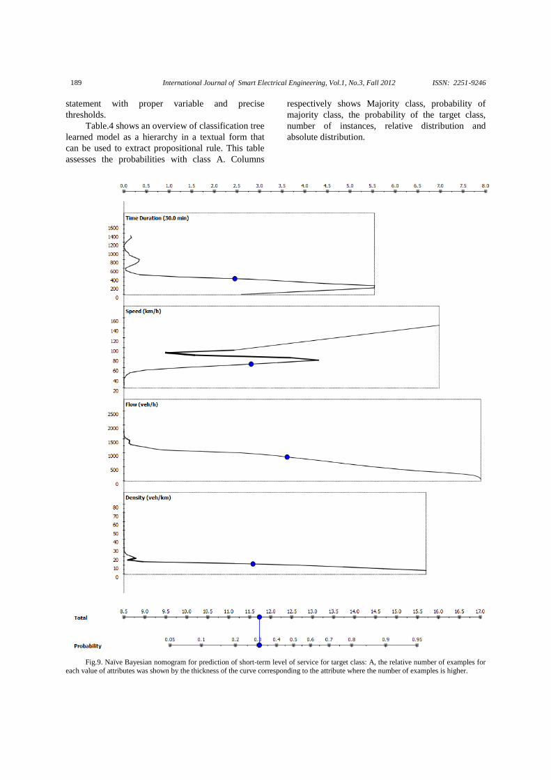
3.2. Naïve Bayesian Nomogram

Nomogram is a simple and intuitive, yet useful

and powerful representation of linear models, such as

logistic regression, naive Bayesian classifier and

linear SVM. Fig.4 shows a Naïve Bayesian

nomogram to assess the prediction probability of

class A. In statistical terms, the nomogram plots log

odds ratios for each value of each attribute. For more

information, readers can refer to Mozina & et al.

[31]. The topmost horizontal axis of this diagram

represents the point scores, e.g. the odds ratio, which

are estimated from the training data. To get log odds

ratios for a particular value of the attribute, find the

vertical axis to the left of the curve corresponding to

the attribute. Then imagine a line to the left, at the

point where it hits the curve, turn upwards and read

the number on the top scale. The curve thus shows a

mapping from attribute values on the left to log odds

at the top. The lower part of the nomogram (bottom

two axes of the nomogram) relates the sum of points

as contributed by the known attributes to the class

probability ( ). The Naïve Bayesian nomogram structure

reveals influences of the attribute values to the class

probability. According to Fig.4 Flow has the biggest

potential influence on the prediction probability of

class A, since the corresponding line in the

nomogram for this attribute is the longest. After that

Speed, Density and Time are respectively influential

parameters in the probability of the class A for the

next time interval. This diagram also shows that

effect of Speed and Time is not monotonous.

3.3. Rule Evaluation

Using CN2 model, the number of 527, 353 and

229 if-then rules generated respectively for 10, 15

and 30 min time intervals which correspondingly in

224, 166 and 102 cases the rule quality was greater

than or equal to 0.9 . Table.3 lists 14 rules of the

whole rule set generated by CN2 on 30 min time

interval records. These rules selected by rule quality

threshold 0.9 and coverage threshold 40. For

example, the rule No. 2 that only depends on Speed

and Flow to ensure next state will be in LOS A can

be interesting for indicating maximum flow in free-

flow condition. The rule No. 14 says between 3:30

PM to 5:30 PM if Speed is less than or equal to 63

km and Flow is greater than 1598, LOS will change

to F. Rules like this latter case are interesting in

designing traffic management and traveler

information systems because they declare detailed

International Journal of Smart Electrical Engineering, Vol.1, No.3, Fall 2012 ISSN: 2251-9246

189

statement with proper variable and precise

thresholds.

Table.4 shows an overview of classification tree

learned model as a hierarchy in a textual form that

can be used to extract propositional rule. This table

assesses the probabilities with class A. Columns

respectively shows Majority class, probability of

majority class, the probability of the target class,

number of instances, relative distribution and

absolute distribution.

Fig.9. Naïve Bayesian nomogram for prediction of short-term level of service for target class: A, the relative number of examples for

each value of attributes was shown by the thickness of the curve corresponding to the attribute where the number of examples is higher.

International Journal of Smart Electrical Engineering, Vol.1, No.3, Fall 2012 ISSN: 2251-9246

190

Table.3

Selected Rules (obtained from 30 min time interval records) with Rule quality threshold 0.9 and coverage threshold 40

No. Rule

length

Rule

quality Coverage

Predicted

class Distribution Rule

1 4 0.998 430 A 430.0:0.0:0.0:0.0 IF Time Duration (min)<=240 AND Flow (veh/h)<=774 AND Time Duration (min)>30 AND Speed (km/h)>69 THEN

nextState=A

2 2 0.978 43 A 43.0:0.0:0.0:0.0 IF Speed (km/h)<=95 AND Flow (veh/h)<=170 THEN nextState=A

3 3 0.987 74 C 0.0:74.0:0.0:0.0 IF Time Duration (min)>1350 AND Speed (km/h)>65 AND

Flow (veh/h)>42 THEN nextState=C

4 3 0.994 152 C 0.0:152.0:0.0:0.0 IF Speed (km/h)>85 AND Time Duration (min)<=390 AND

Flow (veh/h)>102 THEN nextState=C

5 4 0.981 50 C 0.0:50.0:0.0:0.0 IF Flow (veh/h)>104 AND Speed (km/h)>90 AND Flow

(veh/h)>1264 AND Density (veh/km)<=15 THEN nextState=C

6 4 0.979 45 C 0.0:45.0:0.0:0.0 IF Speed (km/h)>83 AND Time Duration (min)>1050 AND Flow (veh/h)<=1286 AND Flow (veh/h)>1246 THEN

nextState=C

7 6 0.987 73 C 0.0:73.0:0.0:0.0

IF Flow (veh/h)<=1254 AND Density (veh/km)>11 AND

Speed (km/h)>77 AND Time Duration (min)<=390 AND Time Duration (min)>120 AND Speed (km/h)<=84 THEN

nextState=C

8 7 0.986 70 C 0.0:70.0:0.0:0.0

IF Density (veh/km)<=15 AND Time Duration (min)>270 AND Time Duration (min)<=360 AND Density (veh/km)>7

AND Speed (km/h)>74 AND Speed (km/h)<=82 AND Flow

(veh/h)>636 THEN nextState=C

9 4 0.979 46 D 0.0:0.0:46.0:0.0

IF Time Duration (min)<=900 AND Density (veh/km)<=19

AND Density (veh/km)>18 AND Density (veh/km)<=19

THEN nextState=D

10 7 0.977 41 D 0.0:0.0:41.0:0.0

IF Flow (veh/h)>1356 AND Time Duration (min)<=900 AND

Density (veh/km)>16 AND Density (veh/km)<=22 AND

Speed (km/h)<=76 AND Flow (veh/h)<=1480 AND Flow

(veh/h)>1410 THEN nextState=D

11 5 0.983 58 D 0.0:0.0:58.0:0.0 IF Density (veh/km)>15 AND Time Duration (min)<=900 AND Density (veh/km)<=18 AND Speed (km/h)<=83 AND

Time Duration (min)>750 THEN nextState=D

12 6 0.984 60 D 0.0:0.0:60.0:0.0

IF Flow (veh/h)>1254 AND Density (veh/km)>16AND Speed

(km/h)<=73 AND Time Duration (min)>990 AND Time Duration (min)<=1170 AND Speed (km/h)>67 THEN

nextState=D

13 4 0.988 83 F 0.0:0.0:0.0:83.0

IF Speed (km/h)<=53 AND Flow (veh/h)>1480 AND Density

(veh/km)>37 AND Time Duration (min)<=1170 THEN nextState=F

14 4 0.985 65 F 0.0:0.0:0.0:65.0

IF Speed (km/h)<=63 AND Flow (veh/h)>1598 AND Time

Duration (min)>930 AND Time Duration (min)<=1050 THEN nextState=F

4. Conclusion

In this study, a classification data mining

approach has proposed for the prediction of road

facility’s level of service and producing simple and

easy handling if-then rules. This method can be used

in designing intelligent transportation and expert

systems and in studying of traffic pattern by traffic

engineers.

The results show Classification Tree and Random

Forest have the best result in prediction. The Naïve

Bayesian nomogram also showed that Flow has the

biggest potential influence between other attributes

on the prediction. CN2 model generated some well-

suited if-then rules that can be used in studying of the

traffic pattern.

A considerable number of topics can be investigated

in this area for future work, including: setting

boundary conditions and calibration parameters of

macroscopic simulation models according to predict

LOS, finding road facility characteristics and

recognition effective variable information and

prediction of congestion, designing the decision tree

controller, expert traffic systems and knowledge base

systems based on the generated if-then rules.

International Journal of Smart Electrical Engineering, Vol.1, No.3, Fall 2012 ISSN: 2251-9246

191

Table.4

Hierarchy rules of classification tree with target class: A; Tree size: 615 nodes, 308 leaves

Classification Tree Class P(Class) P(Target) # Inst Distribution (rel) Distribution (abs)

C 0.375 0.173 4121

0.173:0.375:0.306:0.145

713:1547:1263:598

Density (veh/km) <=16.314 C 0.577 0.292 2416 0.292:0.577:0.12

9:0.002 706:1393:311:6

Flow (veh/h) <=899 A 0.752 0.752 896 0.752:0.232:0.01

5:0.001 674:208:13:1

Time Duration (min) <=255 A 0.96 0.96 572 0.960:0.040:0.00

0:0.000 549:23:0:0

Time Duration (min) <=45 C 0.789 0.211 19 0.211:0.789:0.00

0:0.000 4:15:0:0

Flow (veh/h) <=798 A 0.5 0.5 8 0.500:0.500:0.00

0:0.000 4:4:0:0

Flow (veh/h) >798 C 1 0 11 0.000:1.000:0.00

0:0.000 0:11:0:0

Time Duration (min) >45 A 0.986 0.986 553 0.986:0.014:0.00

0:0.000 545:8:0:0

Time Duration (min) >255 C 0.571 0.386 324 0.386:0.571:0.04

0:0.003 125:185:13:1

Flow (veh/h) <=458 A 0.8 0.8 105 0.800:0.171:0.02

9:0.000 84:18:3:0

Flow (veh/h) <=184 A 0.92 0.92 50 0.920:0.020:0.06

0:0.000 46:1:3:0

Flow (veh/h) >184 A 0.691 0.691 55 0.691:0.309:0.00

0:0.000 38:17:0:0

Flow (veh/h) >458 C 0.763 0.187 219 0.187:0.763:0.04

6:0.005 41:167:10:1

Density (veh/km)

<=8.142 C 0.596 0.362 94

0.362:0.596:0.04

3:0.000 34:56:4:0

Density (veh/km)

>8.142 C 0.888 0.056 125

0.056:0.888:0.04

8:0.008 7:111:6:1

Flow (veh/h) >899 C 0.78 0.021 1520 0.021:0.780:0.19

6:0.003 32:1185:298:5

Density (veh/km) <=14.990 C 0.884 0.037 845 0.037:0.884:0.07

7:0.002 31:747:65:2

Time Duration (min)

<=405 C 0.936 0.058 360

0.058:0.936:0.00

6:0.000 21:337:2:0

Speed (km/h)

<=85.242 C 0.891 0.1 211

0.100:0.891:0.00

9:0.000 21:188:2:0

Speed (km/h) >85.242 C 1 0 149 0.000:1.000:0.00

0:0.000 0:149:0:0

Time Duration (min) >405 C 0.845 0.021 485 0.021:0.845:0.13

0:0.004 10:410:63:2

Speed (km/h) <=81.499

D 0.538 0.077 13 0.077:0.231:0.53

8:0.154 1:3:7:2

Speed (km/h) >81.499 C 0.862 0.019 472 0.019:0.862:0.11

9:0.000 9:407:56:0

Density (veh/km) >14.990 C 0.649 0.001 675 0.001:0.649:0.34

5:0.004 1:438:233:3

Time Duration (min)

<=1155 C 0.575 0.002 511

0.002:0.575:0.41

7:0.006 1:294:213:3

Speed (km/h) <=86.899

D 0.556 0 279 0.000:0.434:0.55

6:0.011 0:121:155:3

Speed (km/h) >86.899 C 0.746 0.004 232 0.004:0.746:0.25

0:0.000 1:173:58:0

Time Duration (min) >1155

C 0.878 0 164 0.000:0.878:0.12

2:0.000 0:144:20:0

Speed (km/h)

<=83.418 C 0.783 0 69

0.000:0.783:0.21

7:0.000 0:54:15:0

Speed (km/h) >83.418 C 0.947 0 95 0.000:0.947:0.05

3:0.000 0:90:5:0

Acknowledgement

This research presented in this paper was

supported in part by Intelligent Transportation

System Research Institute (ITSRI). The authors

would like to thank Tehran Traffic control Co. for its

support.

International Journal of Smart Electrical Engineering, Vol.1, No.3, Fall 2012 ISSN: 2251-9246

192

References

[1] Abdulhai, B. P. ,“Short-term traffic flow prediction using neuro-genetic algorithms”. ITS Journal, Vol.7, pp.3-41, 2002.

[2] P. Allaby, B. Hellinga, and Bullock, M. ,“Variable Speed Limits: Safety and Operational Impacts of a Candidate Control

Strategy for an Urban Freeway”, IEEE Intelligent Transportation

Systems Conference. Toronto, Canada, 2006.

[3] Y. Amit, & D. Geman ,“Shape Quantization and Recognition

with Randomized Trees”. NEURAL COMPUTATION, Vol.9, Issue.7, pp.1545-1588, 1997.

[4] F. Attneave ,“Applications of information theory to psychology: a summary of basic concepts, methods, and results”.

Holt, 1959.

[5] M. Ben-Bassat, “Use of Distance Measures, Information

Measures and Error Bounds in Feature Evaluation”, Handbook of

Statistics, Classification, Pattern Recognition and Reduction of Dimensionality, Vol.2, pp.773-791, 1982.

[6] L. Breiman, “Bagging predictors”, Machine Learning, Vol.24, Issue.2, pp.123-140, 1996.

[7] L. Breiman, J. H. Friedman, R. A. Olshen, & C. J. Stone, “Classification and Regression Trees”, Chapman & Hall, New

York, 1984.

[8] L. Brieman, “Random Forests”. Machine Learning,

Vol.45, Issue.1, pp.5-32, 2001.

[9] M. Carey, M. Bowers, “A Review of Properties of Flow–

Density Functions”, Transport Reviews, Vol.32, Issue.1, pp.49-73,

2012.

[10] M. Castro-Neto, Y.-S. Jeong, M.-K. Jeong, & L. Han,”

Online-SVR for short-term traffic flow prediction under typical and atypical traffic conditions”. Expert Systems with Applications,

Vol.36, Issue.3, pp.6164-6173, 2009.

[11] B. Cestnik, “Estimating probabilities: A crucial task in

machine learning”, Ninth European Conference on Artificial

Intelligenc, Stokholm, pp.147-149, 1990.

[12] C. Chen, Y. Wang, L. Li, J. Hu, & Z. Zhang. “The retrieval of

intra-day trend and its influence on traffic prediction”. Transportation Research Part C, Vol.22, Issue(June, 2012),

pp.103-118, 2012.

[13] R. Chrobok, O. Kaumann, J. Wahle, M. Schreckenberg,

“Different methods of traffic forecast based on real data”. European Journal of Operational Research , Vol.155 Issue.3,

pp.558-568, 2004.

[14] P. Clark, R. Boswell, “Rule induction with CN2: Some recent

improvements”. In Y. Kodratoff (Ed.) Proceedings of the 5th

European conference, pp.151-163, 1991.

[15] P. Clark, & T. Niblett, “The CN2 Induction Algorithm.

Machine Learning”, Vol.3, Issue.4, pp.261-283, 1989.

[16] E. Cook, L. Goldman,” Empiric comparison of multivariate

analytic techniques: Advantages and disadvantages of recursive partitioning analysis”, Journal of Chronic Diseases, Vol.37,

pp.721-731, 1984.

[17] T. G. Dietterich., “An Experimental Comparison of Three

Methods for Constructing Ensembles of Decision Trees: Bagging,

Boosting and Randomization”, Machine Learning, Vol.40, Issue.2, pp.139-157, 2000.

[18] S. Dzeroski, B. Cestnik , I. Petrovski., “Using the m-estimate in rule induction”, Journal of Computing and Information

Technology, Vol.1, Issue.1, pp.37-46, 1993.

[19] A. H. Ghods, L. Fu, A. Rahimi-Kian, “An Efficient

Optimization Approach to Real-Time Coordinated and Integrated

Freeway Traffic Control”, IEEE Transactions on Intelligent Transportation Systems, Vol.11, Issue.4, pp.872-884, 2010.

[20] J. Guo, B. Williams, B. Smith, “Data collection time intervals for stochastic short-term traffic flow forecasting”, Transportation

Research Record: Journal of the Transportation Research Board, Issue.2024, pp.18-26, 2007.

[21] J. Han, M. Kamber, J. Pei. “Data Mining Concepts and Techniques”, Morgan Kaufmann; 3rd edition, July 6, 2011.

[22] A. Hegyi, B. Schutter. “Optimal Coordination of Variable

Speed Limits to Suppress Shock Waves”, Transportation Research

Record, No.1852, pp.167-174, 2003.

[23] T. K. Ho, “The Random Subspace Method for Constructing

Decision Forests”, IEEE Transactions on Pattern Analysis and Machine Intelligence Pami, Vol.20, Issue.8, pp.832-844, 1998.

[24] W.-C. Hong., “Traffic Flow Forecasting by Seasonal SVR with Chaotic Simulated Annealing Algorithm”, Neurocomputing, Vol.74, Issue.12-13, pp.2096-2107, 2011.

[25] G. V. Kass.,” An Exploratory Technique for Investigating

Large Quantities of Categorical Data”, Applied Statistics, Vol.29,

Issue.2, pp.119-127, 1980.

[26] N. Lavrac, B. Kavsek, P. Flach, L. Todorovski, “Subgroup

Discovery with CN2-SD”, Journal of Machine Learning Research, Vol.5, pp.153-188, 2004.

[27] J. Li, Q. Chen, D. Ni, H. Wang., “Analysis of LWR Model with Fundamental Diagram Subject to Uncertainty”, Greenshields

75 Symposium. Woods Hole MA: Transportation Research Board,

pp.74-83, 2011.

[28] D. Lili, S. Peeta, Y. Hoon Kim. “An adaptive information

fusion model to predict the short-term link travel time distribution in dynamic traffic networks”. Transportation Research Part B,

Vol.46, pp.235-252, 2012.

[29] W.Y. Loh, Y-S shih., “Split selection methods for

classification trees”, Statistics Sinica, Vol.7, pp.815-840, 1997.

[30] R. Michalski., “On the quasi-minimal solution of the general

covering problem”, 5th Int. Symposium on Information

Processing, pp.125-128, Bled, Yugoslavia 1969.

[31] M. Mozina, J. Demsar, M. Kattan, B. Zupan., “Nomograms

for Visualization of Naive Bayesian Classifier”, Lecture Notes in

Computer Science, Vol.3202, pp.337-348, 2004.

[32] T. Oda., “An algorithm for prediction of travel time using vehicle sensor data”, Third International Conference on Road

Traffic Control, pp.40-44. London, England, 1990.

[33] M. Papageorgiou, I. Papamichail, A. Messmer, Y. Wang.,

“Traffic Simulation with METANET”, Fundamentals of Traffic Simulation, International Series in Operations Research &

Management Science, pp.399-430. New York Dordrecht

Heidelberg London, Springer, 2010.

[34] D. Park, L. R. Rilett, “Forecasting multiple-period freeway link travel times using modular neural networks”. Transportation

Research Record, Vol.1617, pp.63-70, 1998.

[35] J. Quinlan, “Induction of decision trees”, Machine Learning, pp.81-106, 1986.

[36] J. Quinlan, “Simplifying decision trees”. International Journal

of Machine Studies, Vol.27, pp.221-234, 1987.

[37] J. R. Quinlan, “C4.5: Programs for Machine Learning”,

Morgan Kaufmann, 1993.

[38] L. Rokach and O. Maimon. “Decision trees”. In Lior Rokach and Oded Maimon (eds) Data Mining and Knowledge Discovery

Handbook, pp.165-192, Springer, NY, 2010.

[39] L. Rokach, O. Maimon, “Top-Down Induction of Decision

Trees Classifiers — A Survey”, IEEE Transaction on Systems, Man and Cybernetics—part C: applications and reviews, Vol.35,

Issue.4, pp.476-487, 2005.

[40] B. Smith, M. Demetsky,“Traffic flow forecasting:

comparison of modeling approaches”, Journal of Transportation

Engineering, Vol.123, Issue.4, pp.261-266, 1997.

International Journal of Smart Electrical Engineering, Vol.1, No.3, Fall 2012 ISSN: 2251-9246

193

[41] B. Smith, B. Williams, R. Oswald. “Comparison of

parametric and nonparametric models for traffic flow forecasting”, Transportation Research Part C. Emerging Technologies, Vol.10,

Issue.4, pp.303-32, 2002.

[42] “Transportation Research Board”. Highway Capacity Manual.

Washington DC: the National Research Council, 2000.

[43] J. van Lint, “Online Learning Solutions for Freeway Travel Time Prediction”, IEEE Transactions on Intelligent Transportation

Systems, pp.38-47, 2008.

[44] C. Wu, C. Wei, D. Su, M. Chang, J. Ho.,“Travel time

prediction with support vector regression”, Intelligent Transportation Systems, pp.1438-1442, Shanghai, China, 2003.

[45] K. Wunderlich, D. Kaufman, R. Smith,“Travel time

prediction for decentralized route guidance architectures”, IEEE Transactions on Intelligent Transportation Systems, Vol.1, Issue.1,

pp.4-14, 2000.

[46] F. Yang, Z. Yin, H. Liu, B. Ran.,“On line recursive algorithm

for short-term traffic prediction”, Transportation Research Record: Journal of the Transportation Research Board, Vol.1879, pp.1-8,

2004.

[47] J. Yang.,“A Study of Travel Time Modeling Via Time Series

Analysis”, IEEE Conference on Control Applications, pp.855-860, Toronto, Canada, 2005.

[48] X. Zhang, J.Rice,“Short-term Travel Time Prediction”.

Transportation Research Part C, Vol.11, Issue.3-4, pp.187-210,

2003.

[49] Y. Zhang, Y. Liu,“Comparison of Parametric and Nonparametric Techniques for Non-peak Traffic Forecasting”,

World Academic of Science and Engineering Technology, Vol.51, 2009.

[50] M. Zhong, S. Sharma, P. Lingras,“Analyzing the performance

of genetically designed short-term traffic prediction models based

on road types and functional classes”, Lecture Notes in Computer Science, Vol.3029, pp.1133-1145, 2004.