predicting simulation parameters of biological systems...
TRANSCRIPT
Predicting Simulation Parameters of Biological Systems
using a Gaussian Process Model
Xiangxin Zhu, Max Welling
Computer Science, UC Irvine
{xzhu,welling}@ics.uci.edu
Fang Jin, John Lowengrub
Mathematics, UC Irvine
{fjin,lowengrb}@math.uci.edu
Abstract
Finding optimal parameters for simulating biological systems is usually a very difficult
and expensive task in systems biology. Brute force searching is infeasible in practice due to
the huge (often infinite) search space. In this paper, we propose predicting the parameters
efficiently by learning the relationship between system outputs and parameters using regres-
sion. However, the conventional parametric regression models suffer from two issues, thus
are not applicable to this problem. First, restricting the regression function as a certain fixed
type (e.g. linear, polynomial, etc.) introduces too strong assumptions that reduce the model
flexibility. Second, conventional regression models fail to take into account the fact that a
fixed parameter value may correspond to multiple different outputs due to the stochastic
nature of most biological simulations, and the existence of a potentially large number of
other factors that affect the simulation outputs. We propose a novel approach based on a
Gaussian process model that addresses the two issues jointly. We apply our approach on a
tumor vessel growth model and the feedback Wright-Fisher model. The experimental results
show that our method can predicts the parameter values of both of the two models with
high accuracy.
1 Introduction
Systems biology is a rapidly growing research field that aims to understand and model the
interactions between the components of biological systems. Their approach often involves
the development of mechanistic and probabilistic models, control theory, and simulations.
However, due to the large number of parameters, variables and constraints in biology sys-
tems, it’s usually very difficult to find the optimal parameter values directly.
1

In a tumor growth model (we will describe the details later), for example, one key
parameter, the diffusion constant, plays a crucial role in controlling the growth speed and
the structure of vessel networks in tumors. How can we efficiently find the optimal value
for it that generates a given simulation result? One possible way could be, rather than
doing brute force search, finding the relationship between the diffusion constant on the one
hand and the system’s output features on the other, using regression. We can then predict
the optimal parameter value using the system’s observed outputs as input to the learned
regression function.
0.1 0.12 0.14 0.16 0.180
5
10
15
20
Sim
ula
tio
n p
ara
me
ter
(diffu
sio
n c
on
sta
nt)
Simulation outputs
?
Figure 1: One feature of simulation outputs versus a simulation parameter (diffusionconstant in the tumor growth model we use). Black dots denote observed data.Given a set of simulation outputs (plotted in red dots), we want to predict thebest parameter value that most likely generated them. Note that the simulationoutput varies even given a fixed parameter value due to the stochastic nature of thesimulation, and a given output could potentially be generated by more than oneparameter value, which makes the conventional regression models not applicable.
However, the conventional parametric regression model, y = f(x, θ)+ε, is not suitable in
this case, and the reason is two-fold. First, usually little is known about what is the correct
form of the function f that describes the relation between the simulation parameters and
the system outputs. It is not reasonable to restrict too much the form of functions that we
consider. If we are using a model based on a certain class of functions (e.g. linear functions)
and the target function can not be well modeled by this class, then the prediction accuracy
will be poor. Second, a fixed parameter value may correspond to multiple different outputs
due to the stochastic nature of the simulation of most biological systems, and the existence of
potentially large number of other parameters which may vary from one simulation to another
(see Fig.1). In other words, the conventional regression model does not take into account
the fact that a set of inputs to the regression model xi can correspond to a single target y.
2

Any conventional regression model would make different predictions for those different input
features, and therefore not use the (known) information that they really correspond to the
same target. We note that these two issues are a very general ones, and not just limited to
the two biological models we use to demonstrate our approach in this paper. We believe that
they are ubiquitous in biological simulation and other sciences. In this work, we propose
a novel model based on the Gaussian process that is able to address the aforementioned
two problems. As such, we believe our model may find broad applicability in the biology
community.
We apply our approach on two models: a tumor vessel network growth model and the
feedback Wright-Fisher model for reproduction of cells. The experimental results show that
our approach generates accurate predictions on both the two models.
The rest of this paper is organized as follows: In section 2, we briefly introduce the
Gaussian process. In section 3 we propose our novel regression model. We briefly introduce
the two simulation models in section 4 and describe the features we use for regression in
section 5. The detailed experiments and results are presented in section 5. We conclude our
work in section 6.
2 Gaussian Processes
A Gaussian process (GP) [16] is a probability distribution over functions f(·). A GP is
specified by a mean function u(·) and a covariance kernel K(·, ·) which are modeled para-
metrically. Once these are given we can compute the joint probability distribution over any
subset of function values (say a pair of points) as follows.
f(x)
f(x′)
∼ N (
u(x)
u(x′)
, K(x,x) K(x,x
′)
K(x′,x) K(x′,x′)
) (1)
Hence all finite dimensional marginal distributions over subsets of function values are Gaus-
sian distributed. Moreover, the covariance kernel is constructed such that points that are
further away from each other are less correlated while points close together are strongly
and positively correlated. This ensures that the functions we consider are smooth at small
distance scales. The mean function is used to bias the functions to the type of functions one
expects to encounter a priori.
While a GP is a prior specification of what functions we expect, the data will transform
that into a posterior distribution over functions that agree with the evidence provided by the
data. Note moreover that the GP also quantifies the uncertainty over functions consistent
with the data. In other words, it tells us not only the most likely regression curve but also
3
a one standard deviation uncertainty band within which the real function may be found.
This is clearly a desirable property.
To compute the posterior probability given data we split our points into training points
{xi,yi} and a testing point x∗, where yi is the observed function value subject to noise
corruption, yi = f(xi) + ε, ε ∼ N (0, σ2I). The joint distribution over training and testing
points is then,
f
f∗
∼ N (
u
u∗
, K KT
∗
K∗ K∗∗
) (2)
while y|f ∼ N (0, σ2I).
Using Bayes rule, we can then compute the posterior of the unseen test case given the
observed data. The posterior can be written in closed-form:
p(f∗|y,x,x∗) = N (u∗ +K∗[K + σ2I]−1(y − u), K∗∗ −K∗[K + σ2I]−1KT∗ ) (3)
A GP is a non-parametric model, which means we do not restrict ourselves to a specific
form or parametrized family of functions. Instead our ”inductive bias” is expressed by
stating something about the smoothness of the functions we like to admit. This means our
inductive bias is weak, or in other words: “we let the data speak”. However, too much
flexibility in a model class means that we may easily overfit to the noise of the data. In a
GP one is protected against overfitting because the parameters in the mean function and
the covariance kernel are not estimated but integrated over. Thus, there is really no fitting
of parameters at all. There is no free lunch of course, and too large a model class may
simply lead to very large uncertainties in ones posterior predictions. Thus, we see that more
inductive bias will allow us to learn more from fewer data points but if our inductive bias
is wrong then we may bias our answer in the wrong direction. We express our inductive
bias by 1) choosing a GP in the first place, 2) choosing a mean function and covariance
kernel and 3) placing priors over the hyper-parameters that govern the mean and covariance
functions.
3 Gaussian Process with Multiple Inputs per Target
As we alluded to before, the situation we face when estimating the parameters from multiple
stochastic simulations is that we now have potentially many inputs corresponding a single
target. In this section, we propose a modified Gaussian process model with multiple inputs
per target to address this issue.
4
3.1 Modeling multiple inputs
We will say that our data comes in groups D = {(Xi, yi)}ci=1 where c is the number of the
data groups and Xi = [x1i , . . . ,x
ji, . . . ,x
Ni
i ] is the set of inputs corresponding to group i.
Also Ni is the number of training samples in ith group and yi is the regression target of the
ith group. Finally, let T = {X∗} be the testing inputs, where X∗ = [x1∗ , . . . ,x
k∗ , . . . ,x
N∗∗ ].
Similarly, N∗ is the number of testing inputs. Assuming that there exists an underlying
intrinsic “center” for each group, the hidden variables Z = {{zi}ci=1, z∗} are introduced to
represent these “centers”. The probability density over the samples in each group is then
modeled by a Gaussian distribution centered at these hidden variable zi:
xji ∼ N (zi,Σi), ∀j (4)
xk∗ ∼ N (z∗,Σ∗), ∀k (5)
Assuming the samples in each group are I.I.D. (independently and identically distributed)
, we thus have:
p(Xi|zi,Σi) =∏j
p(xji|zi,Σi) (6)
p(X∗|z∗,Σ∗) =∏k
p(xk∗ |z∗,Σ∗) (7)
3.2 Gaussian process on the hidden variables
We assume that the value of the noisy regression targets yi depend on the hidden variables
as follows: yi = f(zi) + ε, ε ∼ N (0, σ2n). The function f is modeled as a Gaussian process
(see section 2),
p({fi}ci=1, f∗|{zi}ci=1, z∗) = N (u,
K KT∗
K∗ K∗∗
) (8)
where u = [u1, . . . , uc, u∗] is a vector that denotes the mean function. We model this mean
function as follows,
ui = exp(wT
zi
1
) (9)
where w is a (d+ 1)× 1 vector of parameters. A “1” is appended to z to model an overall
scaling factor.
5
Furthermore,
K KT∗
K∗ K∗∗
is the covariance matrix, whose elements are defined as:
K =
k(z1, z1) k(z1, z2) · · · k(z1, zc)
k(z2, z1) k(z2, z2) · · · k(z2, zc)
......
. . ....
k(zc, z1) k(zc, z2) · · · k(zc, zc)
c×c
(10)
K∗ = [k(z∗, z1), k(z∗, z2), · · · , k(z∗, zc)]1×c (11)
K∗∗ = k(z∗, z∗) (12)
and where k(·, ·) is the covariance kernel function. In this paper we have adopted the Matern
covariance function with noise, which is defined as:
k(za, zb) = σ20(1 +
√3‖za − zb‖
l) exp(−
√3‖za − zb‖
l) (13)
Putting everything together the joint probability of the training data D = {(Xi, yi)}ci=1,
the testing inputs T = {X∗}, the hidden variables Z = {{zi}ci=1, z∗}, the model parameters
Θ = {ψK,w, σn,Σi,Σ∗}, the hidden variables F = {{fi}ci=1} and the prediction target f∗
can be written as:
p(D, T ,Z,Θ,F , f∗) = (14)[∏i
p(Xi|zi,Σi) p(zi) p(Σi)]p(X∗|z∗,Σ∗) p(z∗) p(Σ∗)×
p({fi}ci=1, f∗|{zi}ci=1, z∗)
[∏i
p(yi|fi)]p(w) p(ψK) p(σn)
In Appendix A we provide more details about the model parameters Θ = {ψK,w, σn,Σi,Σ∗}
and the priors we used for them. The graphical representation of our model is given in Fig. 2.
6

Figure 2: The graphical representation of our GP model
3.3 Regression
Our goal is to compute the probability distribution for the variable f∗. Starting from the
joint distribution Eqn. 14 we find,
p(f∗|D, T ) (15)
=
∫∫∫Z,Θ,F
p(f∗,Z,Θ,F|D, T ) dZ dΘ dF (16)
=
∫∫Z,Θ
p(f∗|Z,Θ,D, T ) p(Z,Θ|D, T ) dZ dΘ (17)
The integral of Eqn. 17 is composed of two terms. The first term p(f∗|Z,Θ,D, T ) is the
posterior of a standard Gaussian process that can be computed using Eqn. 3. The second
term p(Z,Θ|D, T ), which is the posterior of the hidden variables and the model parameters
given the observed data and testing inputs, has a very complicated form and thus can not
be calculated analytically. Therefore computing the exact value of Eqn. 17 is non-trivial.
However, the integration of Eqn. 17 can be approximated by sampling from p(Z,Θ|D, T ):
p(f∗|D, T ) (18)
=
∫∫Z,Θ
p(f∗|Z,Θ,D, T ) p(Z,Θ|D, T ) dZ dΘ (19)
≈ 1
N
N∑s=1
p(f∗|Z(s),Θ(s),D, T ) (20)
where Z(s) and Θ(s) is a sample drawn from the posterior distribution p(Z,Θ|D, T ). When
7
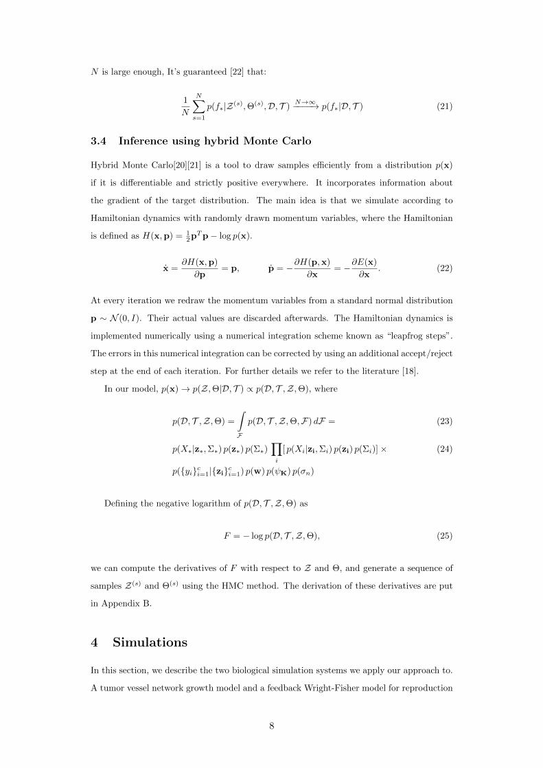
N is large enough, It’s guaranteed [22] that:
1
N
N∑s=1
p(f∗|Z(s),Θ(s),D, T )N→∞−−−−→ p(f∗|D, T ) (21)
3.4 Inference using hybrid Monte Carlo
Hybrid Monte Carlo[20][21] is a tool to draw samples efficiently from a distribution p(x)
if it is differentiable and strictly positive everywhere. It incorporates information about
the gradient of the target distribution. The main idea is that we simulate according to
Hamiltonian dynamics with randomly drawn momentum variables, where the Hamiltonian
is defined as H(x,p) = 12pTp− log p(x).
x =∂H(x,p)
∂p= p, p = −∂H(p,x)
∂x= −∂E(x)
∂x. (22)
At every iteration we redraw the momentum variables from a standard normal distribution
p ∼ N (0, I). Their actual values are discarded afterwards. The Hamiltonian dynamics is
implemented numerically using a numerical integration scheme known as “leapfrog steps”.
The errors in this numerical integration can be corrected by using an additional accept/reject
step at the end of each iteration. For further details we refer to the literature [18].
In our model, p(x)→ p(Z,Θ|D, T ) ∝ p(D, T ,Z,Θ), where
p(D, T ,Z,Θ) =
∫F
p(D, T ,Z,Θ,F) dF = (23)
p(X∗|z∗,Σ∗) p(z∗) p(Σ∗)∏i
[ p(Xi|zi,Σi) p(zi) p(Σi)]× (24)
p({yi}ci=1|{zi}ci=1) p(w) p(ψK) p(σn)
Defining the negative logarithm of p(D, T ,Z,Θ) as
F = − log p(D, T ,Z,Θ), (25)
we can compute the derivatives of F with respect to Z and Θ, and generate a sequence of
samples Z(s) and Θ(s) using the HMC method. The derivation of these derivatives are put
in Appendix B.
4 Simulations
In this section, we describe the two biological simulation systems we apply our approach to.
A tumor vessel network growth model and a feedback Wright-Fisher model for reproduction
8
of cells.
4.1 Tumor vessel network growth model
The development of a tumor-induced neovasculature network is modeled using a lattice-free,
discrete framework developed in [2] together with several modifications that are described
below. The angiogenesis model generates a vascular network regulated by tumor angiogenic
factors (TAF), e.g. [8]. Here, we model TAF using a continuum variable that describes
the net effect of pro-angiogenic regulators. The concentration of TAFs, denoted by c, is
governed by the diffusion-reaction equation,
0 = Dc∇2c− βdc+ Scφh(csat − c) (26)
where the diffusion constant Dc is the key parameter in the model we would like to predict
using regression. Refer to Appendix C for more details of this equation.
The new capillaries form randomly at sprouts near the tumor boundary following the
concentration of TAFs. Vessels are described in terms of the trajectories taken by migrating
endothelial cells [4]. A stochastic equation is prescribed for the leading endothelial cell at
the vessel tip that describes the motion as a biased random walk:
dx
dt= se + vrandom, (27)
This is a stochastic model of the chemotaxis of tip endothelial cells up gradients of TAFs.
Find more details in Appendix C.
While there are many parameters in the model (see Tables 5 in Appendix C), we focus
here on the effect of the TAF diffusion coefficient Dc on the developing neovasculature
network and the resulting tumor progression. This models the variable solubility of TAF
isoforms. In particular, it is found that the more soluble isoforms lead to a more disorganized
and less functional vessel network than the more insoluble isoforms.
We performed many simulations with TAF diffusion coefficient Dc ranging from 20 to
1, where we kept all other parameters unchanged but varied the initial tumor shape. In
particular, the initial tumor shape is taken as a small random perturbation of a unit sphere.
A sample of results are shown in Fig. 3. The results are quantified in Fig. 4, where the
tumor volumes [a], the vessel lengths [b] and the ratio of the vessel and tumor volumes [c]
are shown. Note that the vessel volume is obtained by assuming that the vessel network is
a collection of cylindrical vessel segments, with a radius of 0.05 in nondimensional length
(approximately 10µm in dimensional length).
9

[a]
[b]
[c]Figure 3: Tumor and vessel morphologies at times t = 10 (first column), 20 (secondcolumn), 30 (third column) and 50 (fourth column), from left to right. In each row,the TAF diffusivity Dc is different. [a] Dc = 20; [b] Dc = 10; [c]. Dc = 3.
0 10 20 30 40 500
50
100
150
200
250
300
350
400
450
500
time
tum
or
vo
lum
e
Dc=20 viable
Dc=10 viable
Dc=3 viable
(a)
0 10 20 30 40 500
500
1000
1500
2000
2500
3000
time
vessel le
ngth
Dc=20 total
Dc=20 looped
Dc=10 total
Dc=10 looped
Dc=3 total
Dc=3 looped
(b)
0 10 20 30 40 500
0.002
0.004
0.006
0.008
0.01
0.012
time
vessel volu
me v
s v
iable
volu
me
Dc=20 total
Dc=20 looped
Dc=10 total
Dc=10 looped
Dc=3 total
Dc=3 looped
(c)
Figure 4: Details of the simulations shown in Fig. 3. [a]. Tumor volume; [b] Totallength of both looped vessels and the total neovascular network; [c] the ratio of thevessel volume to the tumor volume. The TAF diffusion coefficient Dc is labeled.
10
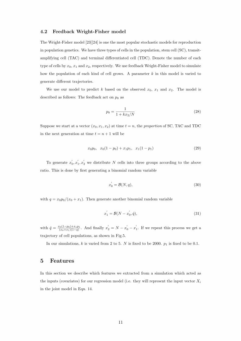
4.2 Feedback Wright-Fisher model
The Wright-Fisher model [23][24] is one the most popular stochastic models for reproduction
in population genetics. We have three types of cells in the population, stem cell (SC), transit-
amplifying cell (TAC) and terminal differentiated cell (TDC). Denote the number of each
type of cells by x0, x1 and x2, respectively. We use feedback Wright-Fisher model to simulate
how the population of each kind of cell grows. A parameter k in this model is varied to
generate different trajectories.
We use our model to predict k based on the observed x0, x1 and x2. The model is
described as follows: The feedback act on p0 as
p0 =1
1 + kx2/N(28)
Suppose we start at a vector (x0, x1, x2) at time t = n, the proportion of SC, TAC and TDC
in the next generation at time t = n+ 1 will be
x0p0, x0(1− p0) + x1p1, x1(1− p1) (29)
To generate x′
0, x′
1, x′
2 we distribute N cells into three groups according to the above
ratio. This is done by first generating a binomial random variable
x′
0 = B(N, q), (30)
with q = x0p0/(x0 + x1). Then generate another binomial random variable
x′
1 = B(N − x′0, q), (31)
with q = x0(1−p0)+x1p1(x0+x1)(1−q) . And finally x
′
2 = N − x′0 − x′
1. If we repeat this process we get a
trajectory of cell populations, as shown in Fig.5.
In our simulations, k is varied from 2 to 5. N is fixed to be 2000. p1 is fixed to be 0.1.
5 Features
In this section we describe which features we extracted from a simulation which acted as
the inputs (covariates) for our regression model (i.e. they will represent the input vector Xi
in the joint model in Eqn. 14.
11

0 100 200 300 400 500 6000
200
400
600
800
1000
1200
1400
1600
1800
2000
t
cell
popu
latio
n
SCTACTDC
Figure 1: Wright-Fisher model generated using parameters p1 = 0.1, N = 2000 and = 5.
1 Feedback Wright-Fisher ModelWe have three types of cells in the population, stem cell (SC), transit-amplifying cell (TAC) andterminal differentiated cell (TDC). Denote the number of each type of cells by x0, x1 and x2,respectively. Denote p0 and p1 as the probability of commitment of SC and TAC, respectively.N = x0 + x1 + x2 is the total population, which is constant.
Feedback
The feedback act on p0 as
p0 =1
1 + x2/N.
How to generate a trajectory?
Suppose we start at a vector (x0, x1, x2) at time t = n, the proportion of SC, TAC and TDCin the next generation at time t = n + 1 will be
x0p0, x0(1 � p0) + x1p1, x1(1 � p1).
To generate x00, x
01, x
02 we distribute N cells into three groups according to the above ratio. This
is done by first generate a binomial random variable
x00 = B(N, q),
with q = x0p0/(x0 + x1). Then generate another binomial random variable
x01 = B(N � x0
0, q),
with q =x0(1 � p0) + x1p1
(x0 + x1)(1 � q). And finally x0
2 = N � x00 � x0
1. Repeat this process we get a trajec-
tory of cell populations as shown by the figure.
Parameters of the model
1
Figure 5: The trajectories of cell population in our simulation with the feedbackWright-Fisher model, using parameters p1 = 0.1, N = 2000 and k = 5.
5.1 Tumor vessel network growth model
Tortuosity: Tortuosity is a property of a curve being tortuous (twisted; having many
turns). Tortuosity of blood vessels is known to be used as a medical sign[13]. There have
been several attempts to quantify this property[14][15]. We propose a new measurement of
tortuosity: non-dominant variance ratio. It is the normalized sum of the variances of nodes
in all non-dominant directions. We apply principal component analysis (PCA) on the 3D
coordinates of all nodes in a branch. The largest eigenvalue corresponds to the variance
in the dominant direction. The non-dominant variance ratio is the sum of all eigenvalues
except the largest one, divided by the sum of all eigenvalues. Fig. 6a illustrates the variances
of the node locations in two orthogonal directions in a 2D plane. In this example, the non-
dominant variance ratio can be computed as σ1
σ0+σ1. It is easy to see that the non-dominant
variance ratio is a dimensionless quantity in the range [0, 1] 1.
The measurement is defined on a vessel branch. The tortuosity of a vessel network is the
average tortuosity values over all branches in the network.
Junction-node ratio: The junction node ratio is the number of junction points divided
by the total number of nodes in the vessel network, where junction points are the nodes that
belong to more than one branch. Fig. 6b illustrates a junction node and non-junction nodes
in a vessel network.
Tortuosity and the junction node ratio are used together to characterize the tumor vessel
network. A predefined list of diffusion constants Dc is chosen. For each of the diffusion
constants, a simulation is run for a fixed amount of time, t = 40 days, and then the features
1By definition, the value of the non-dominant variance ratio in the 3D case won’t be close to 1. It is just aloose upper bound.
12
(a) (b)
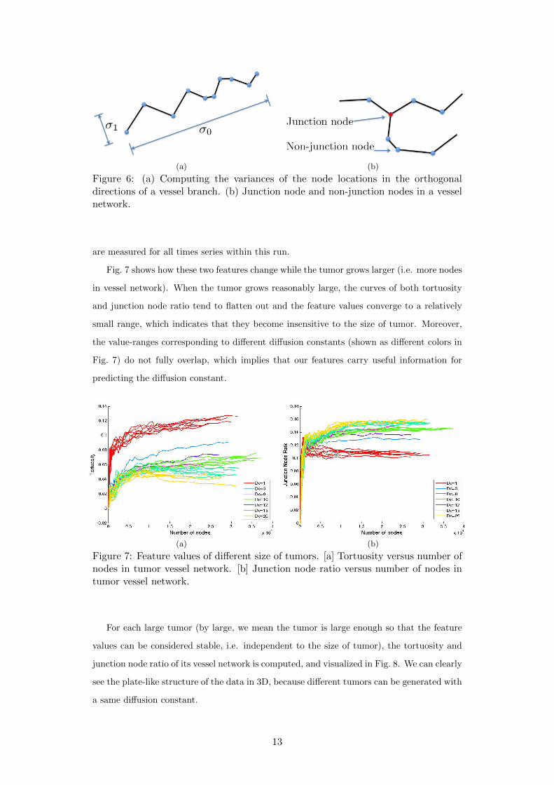
Figure 6: (a) Computing the variances of the node locations in the orthogonaldirections of a vessel branch. (b) Junction node and non-junction nodes in a vesselnetwork.
are measured for all times series within this run.
Fig. 7 shows how these two features change while the tumor grows larger (i.e. more nodes
in vessel network). When the tumor grows reasonably large, the curves of both tortuosity
and junction node ratio tend to flatten out and the feature values converge to a relatively
small range, which indicates that they become insensitive to the size of tumor. Moreover,
the value-ranges corresponding to different diffusion constants (shown as different colors in
Fig. 7) do not fully overlap, which implies that our features carry useful information for
predicting the diffusion constant.
(a) (b)
Figure 7: Feature values of different size of tumors. [a] Tortuosity versus number ofnodes in tumor vessel network. [b] Junction node ratio versus number of nodes intumor vessel network.
For each large tumor (by large, we mean the tumor is large enough so that the feature
values can be considered stable, i.e. independent to the size of tumor), the tortuosity and
junction node ratio of its vessel network is computed, and visualized in Fig. 8. We can clearly
see the plate-like structure of the data in 3D, because different tumors can be generated with
a same diffusion constant.
13
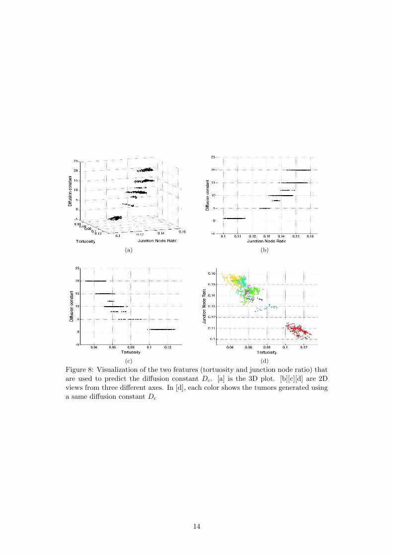
(a) (b)
(c) (d)
Figure 8: Visualization of the two features (tortuosity and junction node ratio) thatare used to predict the diffusion constant Dc. [a] is the 3D plot. [b][c][d] are 2Dviews from three different axes. In [d], each color shows the tumors generated usinga same diffusion constant Dc
14

5.2 Feedback Wright-Fisher model
The number of three kinds of cells (SC, TAC and TDC) are used as features to predict the
parameter k in Eqn.28. We visualize the three features and the k values used to generate
them in Fig.9.
(a) (b) (c)
Figure 9: Visualization of the three features (SC, TAC and TDC) that are used topredict k. [a] is stem cell, [b] is transit-amplifying cell, [c] is terminal differentiatedcell
6 Experiments and Results
6.1 Tumor vessels data
Our dataset consists of around 700 data points from 7 distinct diffusion constants (7 groups).
6.1.1 Parameter values
The parameter values we used in the experiment are listed in Tab. 1:
β(m)z 0.5 Λw 3I
β(1)K 1 βΣim 1
β(2)K 2 βΣ∗m 1
βσn 0.5
Table 1: The parameter values we used in the experiments.
At the beginning of the HMC sampling process, F (0) and Θ(0) are initialized at their
maximum likelihood values. µw is initialized using a simple linear least-square regression.
6.1.2 Prediction results
We use a leave-one-out test mechanism. At every round we pick one group of data-points
corresponding to one value of Dc as test input, and the rest for training. The ground truth
15
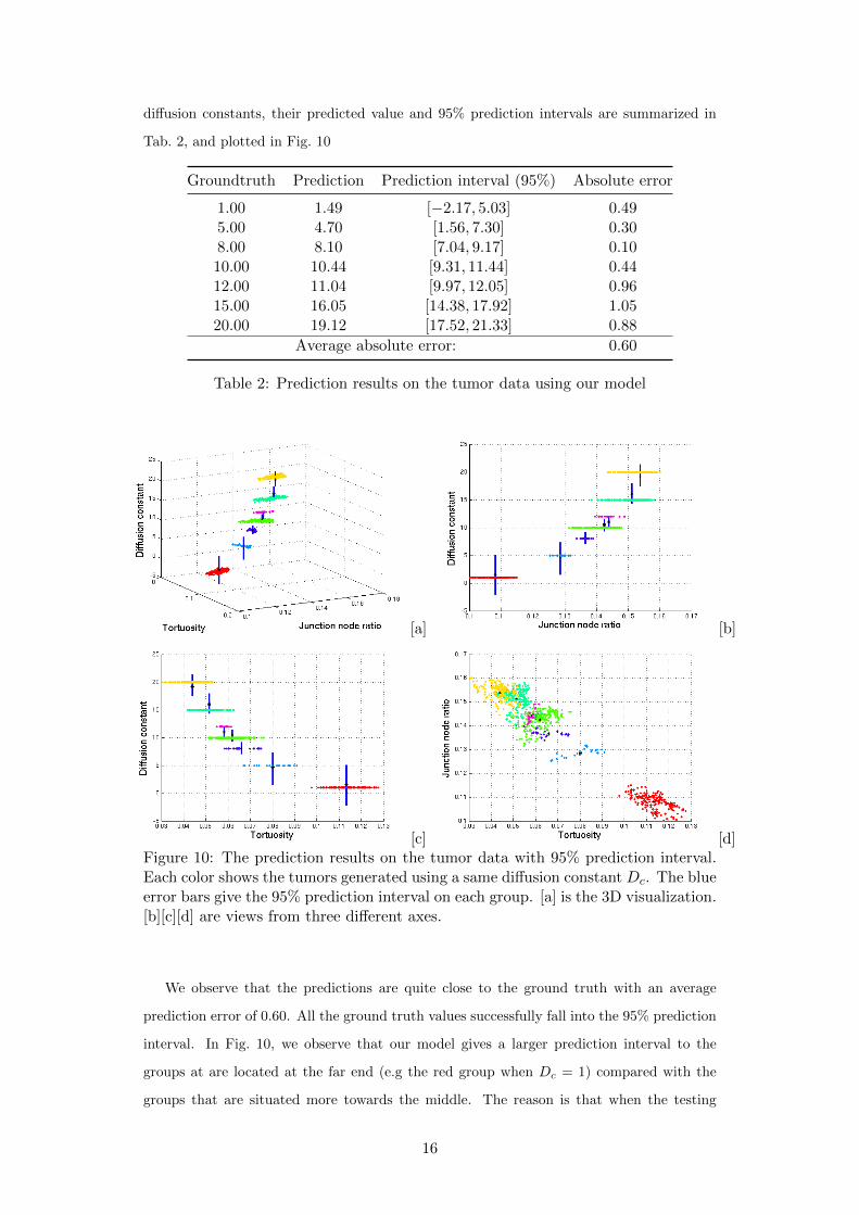
diffusion constants, their predicted value and 95% prediction intervals are summarized in
Tab. 2, and plotted in Fig. 10
Groundtruth Prediction Prediction interval (95%) Absolute error
1.00 1.49 [−2.17, 5.03] 0.495.00 4.70 [1.56, 7.30] 0.308.00 8.10 [7.04, 9.17] 0.1010.00 10.44 [9.31, 11.44] 0.4412.00 11.04 [9.97, 12.05] 0.9615.00 16.05 [14.38, 17.92] 1.0520.00 19.12 [17.52, 21.33] 0.88
Average absolute error: 0.60
Table 2: Prediction results on the tumor data using our model
[a] [b]
[c] [d]Figure 10: The prediction results on the tumor data with 95% prediction interval.Each color shows the tumors generated using a same diffusion constant Dc. The blueerror bars give the 95% prediction interval on each group. [a] is the 3D visualization.[b][c][d] are views from three different axes.
We observe that the predictions are quite close to the ground truth with an average
prediction error of 0.60. All the ground truth values successfully fall into the 95% prediction
interval. In Fig. 10, we observe that our model gives a larger prediction interval to the
groups at are located at the far end (e.g the red group when Dc = 1) compared with the
groups that are situated more towards the middle. The reason is that when the testing
16

points are relatively far away from the training data, our GP model is less confident on its
predictions than when the data are surrounded by other data. In other words, interpolation
is easier than extrapolation.
6.2 Feedback Wright-Fisher model
6.2.1 Parameter Values
The parameter values we used in the experiment are listed in Tab. 3: At the beginning of
β(m)z 5 Λw 0.005I
β(1)K 3 βΣim 5
β(2)K 0.05 βΣ∗m 5
βσn 0.05
Table 3: The parameter values we used in the experiments.
the HMC sampling process, F (0) and Θ(0) are initialized with their maximum likelihood
estimations. µw is initialized with simple linear least-square regression.
6.2.2 Prediction results
We use again a leave-one-out test mechanism. The ground truth value of k, as well as its
prediction by the model and the 95% prediction intervals are summarized in Tab. 4, and
plotted in Fig. 11
Groundtruth Prediction Prediction interval (95%) Absolute error
2.00 2.16 [0.90, 3.71] 0.162.50 2.51 [1.73, 3.29] 0.013.00 2.98 [2.23, 3.74] 0.023.50 3.61 [2.91, 4.31] 0.114.00 4.11 [3.41, 4.77] 0.114.50 4.44 [3.76, 5.14] 0.065.00 4.82 [4.01, 5.59] 0.18
Average absolute error: 0.09
Table 4: Prediction results on the feedback Wright-Fisher data using our model
Again, our predictions are very accurate with a small average prediction error of 0.09.
All the ground truth values successfully fall into the 95% prediction interval.
7 Conclusion
We have proposed a fully (nonparametric) Bayesian approach to regression in a situation
where multiple inputs (covariates) correspond to a single label (response). In this work
17

(a) (b) (c)
Figure 11: The prediction results of k with prediction interval. The blue error barsgive the 95% prediction interval on each group. [a][b][c] show the same result butfrom different dimension of the features.
we have focussed on the prediction of the diffusion constant which was an important input
parameter for the simulation of tumor growth. We have used two properties of the tumor
vessel network, namely tortuosity and Junction Node Ratio to predict the diffusion constant.
As a second experiment we have looked at the prediction of k in the feedback Wright-Fisher
model for the number of stem cells, transit-amplifying cells and terminal differentiated cells.
In both cases our predictions were very accurate and the ground truths lie within the 95%
prediction interval predicted by our model. Note that these uncertainty bands provide very
useful information beyond the prediction value itself.
This seems the first fully Bayesian treatment of regression with multiple covariates per
response value. However, we believe this type of regression problem is ubiquitous in biology
because due to noise or extreme sensitivity to initial conditions (a.k.a. chaos) in the gener-
ating process we are often faced with a many-to-one correspondence between covariates and
response variables. As such, our method may find widespread application in this scientific
discipline.
References
[1] S.M. Wise, J.S. Lowengrub, H.B. Frieboes, V. Cristini, “Three-dimensional multispecies
nonlinear tumor growth: Model and numerical method”, J. Theor. Biol. vol. 253, 524-
543, 2008. 23, 24
[2] H.B. Frieboes, F. Jin, Y.-L. Chuang, S.M. Wise, J.S. Lowengrub, V. Cristini, “ Three
dimensional multispecies nonlinear tumor growth II: Tumor invasion and angiogenesis”,
J. Theor. Biol., vol. 264, 1254-1278, 2010. 9, 23, 24
[3] V. Cristini, J.S. Lowengrub, Multiscale modeling of cancer: An integrated experimen-
tal and mathematical modeling approach, Cambridge University Press, Cambridge UL,
18

2010. 23
[4] A.R.A. Anderson and M.A.J. Chaplain, “ Continuous and discrete mathematical models
of tumor-induced angiogenesis”, Bull. Math. Biol., vol. 60, 857-900, 1998. 9, 23, 24
[5] S.R. McDougall, A.R.A. Anderson, M.A.J. Chaplain, J. Sherratt “ Mathematical mod-
elling of flow through vascular networks: implications for tumour-induced angiogenesis
and chemotherapy strategies”, Bull. Math. Biol., vol. 64, 673-702, 2002. 23
[6] M.J. Plank and B.D. Sleeman, “ A reinforced random walk model of tumour angiogen-
esis and anti-angiogenic strategies”, Math. Med. Biol., 2003. 23, 24
[7] M.J. Plank and B.D. Sleeman, “ Lattice and non-lattice models of tumour angiogene-
sis”, Bull. Math. Biol., vol. 66, 1785-1819, 2004. 23, 24
[8] S. Takano, Y. Yoshii, S. Kondo, H. Suzuki, T. Maruno, S. Shirai, T. Nose, “ Concen-
tration of vascular endothelial growth factor in the serum and tumor tissue of brain
tumor patients”, Cancer Res., vol. 56, 2185-2190, 1996. 9, 23
[9] J.S. Lowengrub, H.B. Frieboes, F. Jin, Y.-L. Chuang, X. Li, P. Macklin, S.M. Wise, V.
Cristini, “ Nonlinear modeling of cancer: Bridging the gap between cells and tumors”,
Nonlinearity, vol. 23, R1-R91, 2010. 24
[10] M.A.J. Chaplain, S.R. McDougall, A.R.A. Anderson, “ Mathematical modeling of tu-
mor induced angiogenesis”, Ann. Rev. Biomed. Eng., vol. 8, 233-257, 1006. 24
[11] A.R. Pries, M. Hopfner, F. le Noble, M.W. Dewhirst, T.W. Secomb, “ The shunt
problem: Control of functional shunting in normal and tumor vasculature”, Nat. Rev.
Cancer, vol. 10, 587-593, 2010. 24
[12] S. Lee, S.M. Jilani, G.V. Nikolova, D. Carpizo and M.L. Iruela-Arispe, “ Processing of
VEGF-A by matrix metalloproteinases regulates bioavailability and vascular patterning
in tumors”, J. Cell Biol., vol. 169, 681-691, 2006. 25
[13] D. McDonald, “Significance of blood vessel leakiness in cancer”, Cancer research, vol.
62, 5381-5385, 2002 12
[14] E. Bullitt et al. “ Measuring Tortuosity of the Intracerebral Vasculature From MRA
Images”, IEEE Transactions on Medical Imaging, vol. 22, No.9, September 2003 12
[15] W. Hart et al. “ Measurement and classification of retinal vascular tortuosity”, Inter-
national Journal of Medical Informatics, No. 53, pp. 239252, 1999. 12
[16] C. Rasmussen and C. Williams, Gaussian Processes for Machine Learning,,2006. 3
[17] R. Neal. “ Monte Carlo Implementation of Gaussian Process Models for Bayesian Re-
gression and Classification”, Technical Report 9702, Dept. of statistics and Dept. of
Computer Science, University of Toronto, January 1997.
[18] R. Neal. “Probabilistic Inference Using Markov Chain Monte Carlo Methods”, Technical
Report CRG-TR-93-1, Dept. of Computer Science, University of Toronto, 1993 8
19
[19] E Bullitt et al. “ Vessel Tortuosity and Brain Tumor Malignancy”, Academic Radiology,
Vol 12, No 10, October 2005
[20] S. Duane, A. Kennedy, B. Pendleton, and D. Roweth, “Hybrid Monte Carlo”, Physics
Letters B, 195:2, 216222, 1987. 8
[21] Christophe Andrieu et al. “An Introduction to MCMC for Machine Learning”, Machine
Learning, 50, pp 5-43, 2003 8
[22] D. Freedman, R. Purves and R. Pisani, Statistics, 3rd edition, W.W. Norton & Com-
pany, 1998 8
[23] R. Fisher, The genetical theory of natural selection. Clarendon Press, Oxford, 1930 11
[24] S. Wright, “Evolution in Mendelian populations”. Genetics. 16:97-159, 1931 11
Appendices
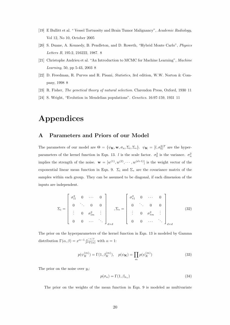
A Parameters and Priors of our Model
The parameters of our model are Θ = {ψK,w, σn,Σi,Σ∗}. ψK = [l, σ20 ]T are the hyper-
parameters of the kernel function in Eqn. 13. l is the scale factor. σ20 is the variance. σ2
n
implies the strength of the noise. w = [w(1), w(2), · · · , w(d+1)] is the weight vector of the
exponential linear mean function in Eqn. 9. Σi and Σ∗ are the covariance matrix of the
samples within each group. They can be assumed to be diagonal, if each dimension of the
inputs are independent.
Σi =
σ2i1 0 · · · 0
0. . . 0 0
... 0 σ2im
...
0 0 · · · . . .
d×d
,Σ∗ =
σ2∗1 0 · · · 0
0. . . 0 0
... 0 σ2∗m
...
0 0 · · · . . .
d×d
(32)
The prior on the hyperparameters of the kernel function in Eqn. 13 is modeled by Gamma
distribution Γ(α, β) = xα−1 e−x/β
βαΓ(α) with α = 1:
p(ψ(m)K ) = Γ(1, β
(m)K ), p(ψK) =
∏m
p(ψ(m)K ) (33)
The prior on the noise over yi:
p(σn) = Γ(1, βσn) (34)
The prior on the weights of the mean function in Eqn. 9 is modeled as multivariate
20

Gaussian distribution with diagonal covariance matrix:
p(w) = N (µw,Λw) (35)
The prior on the diagonal element of Σi and Σ∗ is modeled by Gamma distribution:
p(σ2im) = Γ(1, βΣim), p(σ2
∗m) = Γ(1, βΣ∗m) (36)
Assuming that the elements on the diagonal are independent, p(Σi) and p(Σ∗) can be
written as:
p(Σi) =∏m
p(σ2im), p(Σ∗) =
∏m
p(σ2∗m) (37)
Let zi = [z(1)i , . . . , z
(m)i , . . . , z
(d)i ]T , z∗ = [z
(1)∗ , . . . , z
(m)∗ , . . . , z
(d)∗ ]T . The prior on each dimen-
sion of the hidden variables is modelled to be Gamma-distributed:
p(z(m)∗ ) = p(z
(m)i ) = Γ(1, β(m)
z ) (38)
Notice that β(m)z depends on the dimension index m but is independent to the group index
i.
Since the dimensions of the inputs are independent, p(zi) and p(z∗) can be written as:
p(zi) =∏m
p(z(m)i ), p(z∗) =
∏m
p(z(m)∗ ) (39)
B Derivatives of F
Derivatives of F with respect to Z and Θ for HMC.
21
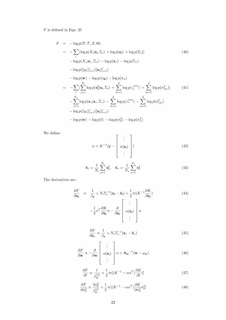
F is defined in Eqn. 25
F = − log p(D, T ,Z,Θ)
= −∑i
[ log p(Xi|zi,Σi) + log p(zi) + log p(Σi)] (40)
− log p(X∗|z∗,Σ∗) − log p(z∗) − log p(Σ∗)
− log p({yi}ci=1|{zi}ci=1)
− log p(w) − log p(ψK)− log p(σn)
= −∑i
[
Ni∑j=1
log p(xji|zi,Σi) +
d∑m=1
log p(z(m)i ) +
d∑m=1
log p(σ2im)] (41)
−N∗∑j=1
log p(x∗|z∗,Σ∗) −d∑
m=1
log p(z(m)∗ ) −
d∑m=1
log p(σ2∗m)
− log p({yi}ci=1|{zi}ci=1)
− log p(w) − log p(l) − log p(σ20) − log p(σ2
n)
We define:
α = K−1(y −
...
u(zi)
...
) (42)
xi =1
Ni
Ni∑j=1
xji, x∗ =
1
N∗
N∗∑j=1
xj∗ (43)
The derivatives are:
∂F
∂zi∝ 1
βz+NiΣ
−1i (zi − xi) +
1
2tr(K−1 ∂K
∂zi) (44)
−1
2αT
∂K
∂ziα− ∂
∂zi
...
u(zi)
...
α
∂F
∂z∗∝ 1
βz+N∗Σ
−1∗ (z∗ − x∗) (45)
∂F
∂w∝ − ∂
∂w
...
u(zi)
...
α+ Λw−1(w − µw) (46)
∂F
∂l∝ l
β(1)K
+1
2tr[(K−1 − ααT )
∂K
∂ll] (47)
∂F
∂σ20
∝ 2σ20
β(2)K
+1
2tr[(K−1 − ααT )
∂K
∂σ20
σ20 ] (48)
22

∂F
∂σ2n
∝ 2σ2n
βσn+
1
2tr[(K−1 − ααT )
∂K
∂σ2n
σ2n] (49)
∂F
∂σ2im
∝ 1
βΣim
+Ni
2σ2im
− 1
2
Ni∑j=1
(xji
(m) − z(m)i )2
σ4im
(50)
∂F
∂σ2∗m∝ 1
βΣ∗m
+N∗
2σ2∗m− 1
2
N∗∑j=1
(xj∗
(m) − z(m)∗ )2
σ4∗m(51)
C Tumor Vessel Network Models
The progression of a vascularized tumor in three dimensions is simulated using a continuum
multispecies tumor model developed by Wise et al. [1] coupled with a lattice-free discrete
model of angiogenesis developed by Frieboes et al. [2]. We briefly describe the models here.
We refer the readers to the references above, and the book by Cristini and Lowengrub [3],
for further details.
C.1 Angiogenesis model
The development of a tumor-induced neovasculature network is modeled using a lattice-free,
discrete framework developed in [2] together with several modifications that are described
below. This builds on earlier work by [4, 5, 6, 7]. The angiogenesis model generates a
vascular network regulated by tumor angiogenic factors (TAF) such vascular endothelial
growth factor (VEGF), e.g. [8]. Here, we model TAF using a continuum variable that
describes the net effect of pro-angiogenic regulators. The concentration of TAFs, denoted
by c, is governed by the diffusion-reaction equation,
0 = Dc∇2c− βdc+ Scφh(csat − c) (52)
where Dc is the diffusivity, βd is the natural decay rate, Sc is the transfer rate of the supply
from the hypoxic cells, and csat denotes the saturation level. The volume fraction of hypoxic
cells φh is defined as the volume fraction of viable cells where the cell substrate is lower than
a specific threshold, which is here set to be the same as the necrotic threshold nV .
The new capillaries form randomly at sprouts near the tumor boundary following the
concentration of TAFs. The scheme first identifies all the sites where the φV < 0.2 and
c > 0.1, which guarantees that the sites are outside the tumor and close to the tumor/host
boundary. Then these sites are weighted by the c and one site is randomly selected from
the list. The frequency of site generation was set to 5 per unit time step (day), which was
calibrated to yield a reasonable number of vessels over the time course of the simulations
presented herein. See [2].
23

Vessels are described in terms of the trajectories taken by migrating endothelial cells
[4]. A stochastic equation is prescribed for the leading endothelial cell at the vessel tip that
describes the motion as a biased random walk:
dx
dt= se + vrandom, (53)
where s = s0|∇c| is the speed of the tip cell with s0 a constant, e = (1−w)eold +w∇c is the
direction of the tip cell with w a weighting factor and eold denotes the previous direction of
the tip cell. Further, vrandom denotes a random direction This is a stochastic model of the
chemotaxis of tip endothelial cells up gradients of TAFs. The endothelial cells just behind
the tip are assumed to proliferate, providing a source of new endothelial cells to populate
the growing vessel [4]. For simplicity, we do not consider the effect of haptotaxis (motion up
gradients of extracellular matrix) here although this can be easily incorporated [4, 6, 7, 2].
A vessel has a fixed probability of branching at each time step. When branching occurs,
the leading endothelial cell splits into two leading cells with the new cells reorienting by a
fixed angle of 30 degrees. The two cells then continue to migrate and proliferate into new
vessels. If the leading cell of one vessel crosses the trail of another vessel from a different
sprout site, then anastomosis may occur (self-intersections are not allowed). This process
forms a closed loop and the corresponding vessel segments between the two sprouts can now
be a source of cell substrates to the surrounding tumor tissue.
The model presented here currently does not include blood flow rates in the vasculature
or the associated morphological changes in the vascular network, such as branching induced
by shear stress. Here, we assume GPF extravasation as soon as the vessels anastomose, which
models the fact that the flow time scale is much faster than the tumor growth time scale.
Simplified models of the blood fluid dynamics in capillary networks have been developed
(e.g, see the reviews [9, 11, 10]) and will be considered in a future work.
C.2 simulation
We perform numerical simulations of the model described in the previous subsection using a
nondimensionalization described in [2]. In particular, space and time are nondimensionalized
by the GPF diffusion length L = (D/νuV )1/2
and the mitosis time scale T = 1/λmV . Note
that because of the relations φT +φH = 1 and φT = φV +φD, we need to solve for only two
variables. Following [1, 2], we solve for φT and φD. Note that we do not need to solve for
φW as this variable is slaved to the growth of the tumor but does not influence the tumor
progression.
While there are many parameters in the model, see Tables 5, we focus here on the effect of
24

νves 0.4 Dc varied
βd 2 Sc 1
csat 1 rves 0.4
εves 0.1 Cves 1
σ√
2 pcrush 0.6
s0 0.2 w 0.9
Table 5: Nondimensional angiogenesis parameters used for the vascularized tumorsimulations shown in Figs. 3 and 4.
the TAF diffusion coefficient Dc on the developing neovasculature network and the resulting
tumor progression. This models the variable solubility of TAF isoforms. For example, it
is known that due to cleavage by matrix metalloproteinases, VEGF isoforms may display
varying degrees of solubility, e.g. see Lee et al. [12]. In particular, it is found that the
more soluble isoforms lead to a more disorganized and less functional vessel network than
the more insoluble isoforms. TAF is set to zero on the boundary of the domain (Dirichlet
boundary condition), which models the intravasation of TAF into the vascular network.
Indeed, soluble forms of tumor-induced TAF can be found in the blood.
We performed many simulations with TAF diffusion coefficient Dc ranging from 20 to
1, where we kept all other parameters unchanged but varied the initial tumor shape. In
particular, the initial tumor shape is taken as a small random perturbation of a unit sphere.
A sample of results are shown in Fig. 3. In the figure, the contours φV = 0.5 of the viable
tumor volume fraction are plotted together with the neovascular network. Blue vessels
denote sprouts which have not yet anastomosed to form a functional network. Vessels
colored red denote the looped, or anaostomosed, vessels that are releasing GFPs into the
tumor microenvironment. As can be clearly seen in the figure, the tumor size and the
number of vessels are decreasing functions of the TAF diffusion coefficient, consistent with
experimental observations. The results are quantified in Fig. 4, where the tumor volumes
[a], the vessel lengths [b] and the ratio of the vessel and tumor volumes [c] are shown. Note
that the vessel volume is obtained by assuming that the vessel network is a collection of
cylindrical vessel segments, with a radius of 0.05 in nondimensional length (approximately
10µm in dimensional length). Again, all these quantities are decreasing functions of the
TAF diffusion coefficient, and increasing functions of time.
25