predicting missing contacts in mobile social networks
TRANSCRIPT

Pervasive and Mobile Computing 8 (2012) 698–716
Contents lists available at SciVerse ScienceDirect
Pervasive and Mobile Computing
journal homepage: www.elsevier.com/locate/pmc
Fast track article
Predicting missing contacts in mobile social networks✩
Kazem Jahanbakhsh ∗, Valerie King, Gholamali C. ShojaComputer Science Department, University of Victoria, B.C., Canada
a r t i c l e i n f o
Article history:Available online 20 July 2012
Keywords:Mobile social networksContact predictionContact graph reconstructionGeographical proximitySocial profilesSocial similarityPopularity
a b s t r a c t
Experimentally measured contact traces, such as those obtained in a conference setting byusing short rangewireless sensors, are usually limitedwith respect to the practical numberof sensors that can be deployed as well as the number of available human volunteers.Moreover, most previous experiments in this field can report only partial contactinformation since not everyone participating in the experiment carries a sensor device.Previously collected contact traces have significantly contributed to the developmentof more realistic human mobility models. This in turn has influenced proposed routingalgorithms for Delay Tolerant Networks where human contacts play a vital role in messagedelivery. By exploiting time-spatial properties of contact graphs as well as the popularityand social information of mobile nodes, we propose a novel method to reconstruct themissing parts of contact graphs where only a subset of nodes are able to sense contacts.
© 2012 Elsevier B.V. All rights reserved.
1. Introduction
The appearance of new wireless technologies has revolutionized the way people communicate and share their contentsuch as videos, photos, andmessages. Delay Tolerant Networks (DTNs) in which nodes can exchange information only whenthey are in close proximity of each other have opened a new and exciting avenue for communication in the emerging socialnetworks. In DTNs, the network is sparse and disconnected most of the time. Thus, most of known protocols for MANETsfail to operate in DTNs where successful delivery of a message strongly relies on human contact patterns.
The availability of contact traces such as [1–3] has allowed researchers to identify the fundamental properties of humanmobility and to propose realistic mobility models [4,5]. By using these mobility models, researchers proposed efficientrouting protocols for DTNs. In particular, SimBet [6], Bubble Rap [7], and Social-Greedy [8] routing algorithms are a fewexamples in which nodes exploit the underlying properties of contact traces for optimal routing. Therefore, the size and thereliability of contact traces are at the core of the ongoing research in DTNs.
Previously, researchers distributed a limited number of short range wireless sensors among a set of people to recordwhen they are in close proximity of each other. More specifically, whenever a person u who carries a sensor device comesinto the close proximity of another person v who carries a wireless sensor or a Bluetooth enabled device, person u’s sensorrecords a contact event with person v. In this paper, we focus on those experiments in which wireless sensors are carried bya set of people to collect their contact events. We can represent the set of events by a directed graph called contact graph,where the nodes are people and the edges are contact events. We call the nodes which carry a sensor device internal nodesand those which carry a Bluetooth enabled device such as cellphones or PDAs external nodes.
In experimental datasets that we have analyzed (see Table 1) we have found that internal nodes recorded a large numberof contacts with external nodes. While internal nodes can record the presence of all other nodes including internal and
✩ A preliminary version of this paper appeared in WoWMoM 2011 conference (Jahanbakhsh et al. (2011) [19]). This work was also supported by NSERCgrant.∗ Corresponding author.
E-mail address: [email protected] (K. Jahanbakhsh).
1574-1192/$ – see front matter© 2012 Elsevier B.V. All rights reserved.doi:10.1016/j.pmcj.2012.07.007

K. Jahanbakhsh et al. / Pervasive and Mobile Computing 8 (2012) 698–716 699
Table 1Real data description.
Dataset Inf 05 Inf 06 MIT Camb Roller
Mobile nodes 41 79 97 36 62Length 3 days 4 days 246 days 11 days 3 hScanning period 120 s 120 s 300 s 600 s 15 sExternal no 206 4321 20698 11367 1050Total contacts 227657 28216 285512 41587 132511Ext. contacts 57056 5757 183135 30714 72365Ext. contacts % 25 20 64 74 55
external ones, the external nodes are not able to detect any contact event. As a result, a large portion of the sampled contactgraphs, specifically the contacts among all external nodes, is missing. Real data which were collected in various settingsshow that people with Bluetooth enabled devices (e.g. external nodes) by far outnumbered those with wireless sensorones.
In this paper, we are interested in reconstructing a complete graph from those partial contact graphs that are collected ina real experiment.We formulate the problemof inferring themissing part of a contact graph as a contact prediction problem,andwe propose severalmethods for predicting themissing contacts. Our proposedmethods predictmissing contacts amongexternal nodes by exploiting the underlying properties of contact graphs. Predicting missing contacts will complete ourobservations about different statistical features of partial contact graphs. In Section 5.3, we particularly show that predictingmissing contacts allows us to restore the communities which otherwise are missing.
In this work, we study a variety of contact traces collected from different social settings such as [1–3,9] for our analysis.Based on the observed time-spatial properties of contact graphs, we propose three different methods to make contactpredictions by computing similarities between neighbor sets of external nodes. We also investigate the effectiveness ofusing nodes’ contact rates for predictingmissing contacts. Furthermore, it was previously shown that the contact probabilitybetween mobile wireless devices is influenced by their owners’ social characteristics [1,10]. We call the set of socialcharacteristics for each user her social profile. In this paper, we present two socially-based methods for predicting missingcontacts, and study their performance using a contact trace collected from a conference setting [2].
Our results show that we can reliably reconstruct the missing parts of contact graphs by using the proposed methods.This enables researchers to expand the existing collected contact traces in order to include the contacts among externalnodes as well. Our solution to the contact prediction problem also sheds light on the way in which people move. While theproblem of link prediction is not new in the context of social networks [11,12], to the best of our knowledge this work is thefirst one that tries to address this problem in the context of mobile social networks, that is, a network consisting of contactsamong a set of mobile users. The main contributions of this paper can be summarized as follows:1. We present the problem of contact prediction in the context of mobile social networks and show how we can study this
problem by using real data from different social settings.2. We propose several methods each of which makes use of one of time-spatial, popularity, or social information to
reconstruct the missing part of a contact graph.3. Finally, we integrate social information with time-spatial information to propose a more effective method for contact
prediction.
The remainder of the paper is organized as follows: Section 2 reviews the recent work in the field. Section 3 defines theproblem to be tackled. Section 4 describes the important properties of contact graphs that can help us predict contacts aswellas proposed methods for contact prediction. The performance results of our methods for different datasets are presentedin Section 5. In Section 6 we explain the performance of time-spatial predictors by a simple mathematical analysis. Finally,Section 7 concludes the paper.
2. Related work
Researchers have proposed several syntheticmobilitymodels based on underlying properties of contact graphs.Musolesiet al. proposed a community-based mobility model (CMM) in which nodes tend to contact other nodes from their owncommunity with higher probability than nodes from different communities [4]. They validated CMM by testing to see ifit produces the same distributions for inter-contact1 and contact duration times as the ones that were observed in realcontact traces. By analyzing human contact and wireless LAN traces, Hsu et al. also introduced the time-variant communitymodel for human mobility [5]. They observed a skewed probability distribution for locations which people visit every dayas well as a time periodic pattern in humanmobility. Most recently, researchers used short range wireless sensors to collectcontact data among soccer players [13]. They proposed a mobility model for soccer games based on the observed statisticalproperties from their contact traces.
The underlying properties of contact graphs play a vital role in the performance of routing algorithms for DTNs. Byusing complex network analysis, researchers found patterns in contact graphs that are similar to those in social graphs.
1 Inter-contact time is the time gap separating two consecutive contacts between the same pair of nodes.

700 K. Jahanbakhsh et al. / Pervasive and Mobile Computing 8 (2012) 698–716
Specifically, they discovered communities and heterogeneous centralities in contact graphs obtained from contact traces.SimBet [6] and Bubble Rap [7] routing algorithmswere proposed based on these observations. Hossmann et al. improved theperformance of SimBet andBubble Rap algorithmsbyproposing a strategy formapping contact graphs to social graphs. Usingtheir strategy, they showed that nodes can make their routing decisions more efficiently [14] than SimBet and Bubble Rap.
In [8] we proposed a routing algorithm called Social-Greedy that exploits the offline social profiles of people for routingmessages in DTNs. In Social-Greedy each mobile node carrying a message forwards its message to those encountered nodesthat are socially closer to the messages’ destinations than itself. We studied the performance of Social-Greedy by using realdata collected from a conference. In this paper we propose a more effective measure to compute the social similarity amongnodes.
The link prediction problem in social networks is similar to the contact prediction problem that we are addressing in thispaper. In the link prediction problem, the goal is to see if we can predict the future links in a social network with a highaccuracy. There are a large number of works in which researchers have addressed the link prediction problem by takinga data mining or machine learning approach. For instance, Nowell et al. studied the link prediction problem in a citationnetwork by extracting several features in order to predict future collaborations among researchers [15]. More interestingly,Hasan et al. extended Nowell’s work by employing several supervised learning classifiers such as Decision Tree and SupportVector Machine [16]. They showed that supervised learning is an efficient way to formulate the link prediction problem insocial networks. Leskovec et al. also used the logistic regression to predict the sign of links in social networks [17].
Recently, we also formulated the contact prediction problem in the context of machine learning [18]. In particular, weemployed two supervised learning algorithms including K-Nearest Neighbor and the Logistic Regression for predictingmissing contacts in mobile social networks. Our performance results showed the applicability of using supervised learningalgorithms for predicting hidden contacts. Interestingly, we discovered that the number of common neighbors and the totaloverlap time are the most significant features in the contact prediction task [18].
This paper is an extended version of our previous work in which we formulated the problem of contact prediction inmobile social networks [19]. We have added the prediction results for a new dataset (i.e. Infocom 2005) to our previousperformance results in [19]. We also compare the densities of MIT contact graphs with Infocom 2006 contact graphs inorder to clarify the performance gap between these two datasets. In addition, here we compare the performance of ourpredictors by using five statistical measures including True Positive Rate, False Positive Rate, Precision, Accuracy, and RootMean Square Error. Computing these five statistical measures for our predictors is essential since they contain TN/FN resultsin addition to TP/FP. The scalability results of the NCN predictor have also been added for both Infocom 2006 and Rollernetdatasets. These results show that the NCN predictor works well even if we decrease the percentage of internal nodes to 20percent. Furthermore, we mathematically explain here why the NCN predictor works well even if there is just one commonneighbor between two external nodes.
3. Problem definition
Acontact event between twousersu and v can be shownby aquadruple (u, v, ts, te) implying that useru’s device detecteduser v’s device in close proximity in the [ts, te] time interval. We assume that every human contact between u and v isrecorded as a contact event by one of the sensors carried by u or v. It is important to note that not every observed contactbetween two devices necessarily means a social interaction between people who carry the devices. For the rest of paper, weonly focus on analyzing those contacts that are collected by wireless sensors in an experiment.
We show all contacts recorded by internal nodes during an experiment using an undirected contact graph G =
(V , Eknown). The reader should note that there is an undirected edge between nodes u and v if at least one of them recordedthe presence of the other one in its proximity. Here, we denote the set of all people participating in the experiment withV = Vint ∪ Vext where Vint and Vext are the sets of internal and external nodes, respectively. We assume that |V | = Nand |Vint | = Nint where Nint < N . We also denote the set of known edges by Eknown where we represent every observedcontact such as (u, v, ts, te) with an undirected edge from node u to node v in G. From the data provided by experimentssuch as those listed in Table 1, we can only construct a partial contact graph. In other words, while the set of edges inEknown ⊂ Vint × (Vint ∪ Vext) is known, all edges between external nodes are missing. Our problem is to infer the missingedges among external nodes by using the available information from the known part of the graph (e.g. Eknown), that is, topredict the edges in Vext × Vext which would have been detected if the nodes in Vext had carried wireless sensors.
4. Reconstructing the contact graph
In this section we describe the essential properties of contact graphs that are useful for contact prediction. We alsopropose three different sets of prediction methods based on the underlying properties of contact graphs. Finally, we explainour main algorithm that makes use of our proposed methods to infer the missing contacts among external nodes.
4.1. Constructing partial contact graphs
Since the collected contact traces change over time (e.g., edges between nodes appear and disappear), we divide theexperiment time into equal intervals of τ seconds called time intervals.We choose τ = c×T where c is a constant integer, and

K. Jahanbakhsh et al. / Pervasive and Mobile Computing 8 (2012) 698–716 701
(a) Time Intervals. (b) Constructing Gk .
Fig. 1. Constructing the partial contact graph Gk .
T is the inquiry interval of wireless sensors that is the time gap between two consecutive samplings. The coefficient c shouldbe chosen carefully according to the dataset setting. Usually c is chosen to be either 1 or 2. Let Λk = [t0 + kτ , t0 + (k+ 1)τ ]
denote the kth time interval where 0 ≤ k < kmax and t0 is the starting time of the experiment (see part (a) of Fig. 1). For eachtime interval Λk, we construct a contact graph Gk by collecting all contacts that were observed by internal nodes in Λk. Weshow the kth contact graph with Gk = (V , Eknown
k ) where V = Vint ∪ Vext is the set of all nodes and Eknownk is the set of all
known edges of Gk (e.g. observed contacts by the internal nodes). In Fig. 1, Gk contains all three contacts e3, e4, and e5 thatare observed by internal nodes in Λk. Our goal is to predict missing edges Eunknown
k ’s by exploiting the information about theknown edges of Gk’s where Eknown
k ⊂ Vint × (Vint ∪ Vext) and Eunknownk ⊂ Vext × Vext .
4.2. Contact graph properties
There are three elements that play essential roles in contact process: (1) time-spatial locality, (2) social similarity, and(3) popularity. Next, we discuss the importance of these elements in the structure of the contact graph.
Time-Spatial locality: A contact between two nodes u and v at time t means that u and v were in close proximity of eachother at time t . If node u records a contactwith node v at time t and node u also records a contactwith nodew at time t+δ fora small δ, we can say that nodes v andw are in a close distance of each other around time t . If two nodes are geographicallyclose, we expect that they are more likely to meet each other in the near future.
Social similarity: Let simsoc(u, v) denote the social similarity between two nodes u and v. We assume that if node u ismore socially similar to v than w (e.g. simsoc(u, w) < simsoc(u, v)), then u is more likely to contact v than w.
Popularity: Popularity in social networks is captured by nodes’ degrees. Let us define a node’s contact rate in time intervalΛk as the number of contacts a node made during Λk. A node’s contact rate in a mobile social network is similar to anode’s degree in a social network, in that it reflects the social role of the device’s owner. For example, if node u’s owneris a conference organizer, it probably has a high contact rate. Thus, if node u has a higher contact rate than v, we can assumethat node u has a higher probability of contacting a given node w than v does.
4.3. Methods based on neighborhood similarity
To predict contacts, one approach is to exploit the underlying properties of contact graphs. Here we want to show thatcontact graphs have a neighborhood-cohesiveness property in which neighbors of a given node have a high probability ofbeing connected to each other. First, we construct the contact graph Gk’s for all time intervals Λk’s as described earlier. Theclustering coefficient of node u in Gk is the fraction of pairs of u’s neighbors that are connected to each other by edges [20].We compute the average clustering coefficient of the contact graph Gk denoted with CCk, by taking the average of clusteringcoefficients of all nodes in Gk. In Fig. 2, we have shown the average clustering coefficients for the contact graphs during thesecond day of Infocom 2006 where τ = 2× T = 4 min. Interestingly, the total average of all computed CCk values is shownto be around 25%.
To justify the neighborhood-cohesiveness property of contact graphs, let us assume that we are running an experimentwith Nint sensors when all of them have similar sensing ranges of r . Moreover, suppose our nodes are uniformly distributedin the experimental region (e.g. a conference hotel). In this graph, there is an undirected edge between two nodes u and vin Λk if their distance is less than r in that time interval (e.g. d(u, v) < r). Now, let us consider the simple scenario shownin part (a) of Fig. 3 where two nodes u and v have detected a common neighbor w at the same time. The existence of links(u, w) and (v, w) implies a geographical proximity between u and v which in turn increases the chance that u and v alsosense each other. It is not hard to see that the number of common neighbors (NCN) between two given nodes u and v isproportional to the intersection area between their radial circles as shown in part (b) of Fig. 3 in which Ou and Cu representthe location of node u in the experimental region and u’s radial circle, respectively. A large NCN for two given nodes impliesa large intersection area between their radial circles which in turn indicates a geographical closeness between them.

702 K. Jahanbakhsh et al. / Pervasive and Mobile Computing 8 (2012) 698–716
Fig. 2. The average clustering coefficient (Infocom06: 9:00 AM to 6:00 PM).
a b
Fig. 3. The effect of common neighbors on geographical proximity.
Now, we discuss three methods that measure the geographical closeness between two nodes based on the intersectionbetween their neighbor sets. In all the following equations, simk(u, v) denotes the similarity between two nodes u and v inΛk, and Nk(u) represents the neighbor set of node uwhich is the set of contacted nodes by u in time interval Λk
simkncn(u, v) =
Nk(u) ∩ Nk(v) (1)
simkjac(u, v) =
Nk(u) ∩ Nk(v)Nk(u) ∪ Nk(v) (2)
simkmin(u, v) =
Nk(u) ∩ Nk(v)
min(Nk(u)
, Nk(v)) . (3)
While Eq. (1) calculates the NCN between a pair of nodes to estimate their closeness, the Eqs. (2) and (3) are thenormalized versions of the NCN method. Eq. (2) (Jacard method) makes use of the Jacard index to measure the similaritybetween the neighbor sets of the given nodes [21]. To clarify the main difference between Eqs. (2) and (3) (Minmethod), letus consider two scenarios. In the first scenario, let us assume that two nodes u and v contacted two similar nodes in timeinterval Λk. Also suppose node u only contacted these two nodes while node v contacted ten nodes including these twocommon nodes in Λk. We may desire a higher significance for the described scenario than if each of u and v had seen sixnodes in Λk where two of these six nodes are in common. Although the Jacard index gives 1
5 for both scenarios, the Minmethod assigns a higher score to the first scenario [12].
4.4. Methods based on social similarity
Considering the importance of the homophily principle in the link formation process in social networks [22], we wantto test the power of social similarity for predicting the contacts among nodes in a mobile social network. In our previouswork, we studied the influence of the similarity of people’s social profiles on their contact probabilities in a conferenceenvironment [8]. Eagle et al. [1] and Mitbaa et al. [10] also found a close relation between human mobility and theirfriendship networks. In this work, we have access to brief social profiles of people who attended the Infocom 2006conference. In these social profiles, people reported their social characteristics. Social characters are classified accordingto different social dimensions such as affiliation, interest, country of birth and so on. For each node u and each socialdimension i, we represent node u’s characteristics in that dimension by a set Γ i
u . We call Γ iu the social characteristic set
of node u in dimension i. For example, node u’s characteristic with respect to research interest dimension can be shownwith a set of research topics such as Γ interests
u = { 1, 2, 3} where 1, 2, 3 can represent DTN, MANET, and Social Networkingareas.

K. Jahanbakhsh et al. / Pervasive and Mobile Computing 8 (2012) 698–716 703
4.4.1. Social similarity based on Jacard indexBy employing the Jacard index, we compute the similarity between two nodes with respect to each social dimension as
follows [8]:
σ ijacard(u, v) =
Γ iu
Γ iv
Γ iu
Γ iv
, (4)
where Γ iu is the social characteristic set of node u for social dimension i, and
Γ iu
is its cardinality. Assuming that we have ddifferent social dimensions for each node, we compute the total social similarity between two nodes by calculating the totalaverage over all d dimensions. Therefore, we obtain the total social similarity between two nodes u and v as below:
simsocjac (u, v) =
di=1
σ ijacard(u, v)
d, (5)
where d is the number of social dimensions. Note that for Infocom 2006 data, the number of available dimensions d = 6, asit will be shown later.
4.4.2. Social similarity based on foci distanceLet us define the social focus as a set of people who share the same research interest, speak the same language, or were
born in the same country. Foci are away of summarizingmany possible reasons that two people contact each other: becausethey are from the same country, have the same affiliation, or share the same interest. Now, suppose in a conference thereare two people u and v who are interested in the Routing research area. Moreover, assume that these two people do nothave any other similarities with respect to other social dimensions. More specifically, they have different affiliations, wereborn in different countries, speak in different languages and so on. Roughly speaking, there is a high probability of these twopeople meeting each other in the conference because both of themmay attend the same sessions. We also can see that theircontact probability has an inverse relationship with the number of people who are interested in the Routing area. Thus, wedefine the Foci distance between two given nodes as the cardinality of the smallest social focus that both of them belongto. In our previous example, the social distance between u and vwith respect to research interest is equal to the number ofconference participants who are also interested in Routing. We define the Foci distance between two given nodes u and v asbelow [23]:
dfoc(u, v) = min |{F |u, v ∈ F}| , (6)
where F is the social focus that both u and v belong to. Considering Eq. (6), we define the Foci similarity between two nodesas follows:
simsocfoc (u, v) =
1dfoc(u, v)
. (7)
4.5. Method based on popularity
Motivated by the preferential attachment model for social networks [24] in which a node u connects to another node vwith a probability that is proportional to v’s degree, we assume that the contact probability between two nodes in a mobilesocial network depends on their individual contact rates. Let λk
u denote the contact rate of node u in the kth time interval thatis the number of its contacts in Λk. We assume that the combined contact rate between two nodes u and v is proportionalto the product of their individual contact rates. Thus, we define the popularity measure between two nodes u and v in timeinterval Λk as below:
simkpop(u, v) = λk
u.λkv. (8)
To compute node u’s contact rate we count the number of u’s contacts in time interval Λk. In Section 5, we employ all sixEqs. (1)–(3), (5), (7) and (8) as our proposed prediction methods to reconstruct the missing parts of contact graphs.
4.6. Reconstruction algorithm
The following steps describe our algorithm for reconstructing the missing parts of Gk’s by selecting one of the previouslypresented prediction methods:
1. First, we generate partial contact graph Gk’s for all k values as we have described in Section 4.1.2. Next, we compute the similarity scores between all pairs of external nodes by using one of our predictionmethods. These
similarity scores basically estimate the contact probabilities among external nodes. Therefore, for each time interval Λkwe obtain quadruples such as (u, v, k, sim(u, v)) where u and v are external nodes, sim(u, v) is the computed similarity

704 K. Jahanbakhsh et al. / Pervasive and Mobile Computing 8 (2012) 698–716
Fig. 4. Simulating a partial contact graph.
score for nodes u and v, and k is the time interval number. We store all quadruples whose similarity scores are greaterthan zero in a similarity list denoted by Lsim for the post-processing step. We repeat the same process for all intervals(0 ≤ k < kmax) and store all the quadruples in the same list.
3. When we finish with all intervals, we sort the Lsim list in a descending order based on computed similarity scores. Thesorted version of the similarity list is our predictor results.
4. To infer themissing contacts, we select the first Ranknumber of predictions from the sorted list of Lsim. For each predictionquadruple, we create an edge between the corresponding external nodes.
5. Performance evaluation
In this section we evaluate the performance of all proposed methods in the previous section by using the availabledatasets. Our ultimate goal is to see which method is more effective for predicting the missing contacts.
5.1. Real data description
Here, we are planning to use contact traces collected from four different social settings. Table 1 describes these datasets.Info 05 and Info 06 datasets were collected from Infocom conferences in 2005 and 2006 respectively. Participants in Info05’s experiment belong to different social communities; however, in the Infocom 2006 participants were specially selectedsuch that 34 people out of 79 were from four research groups [25]. In the Info 06 dataset, participants also reported a briefversion of their social profiles which consisted of (1) nationality, (2) graduate school, (3) languages, (4) affiliations, (5) city &country of residence, and (6) research interests [2]. In the Cambridge dataset (Camb), the wireless sensors were distributedmainly between two groups of undergraduate students from the University of Cambridge, and some graduate studentsfrom a research lab [9]. Note that both Infocom 06 and Cambridge datasets also include data for stationary wireless sensors;however, in this paper we only use the sampled contacts by mobile sensors. While Rollernet dataset (Roller) contains thecontacts from a set of people who participated in a rollerblading tour in Paris [3], Reality dataset (MIT) includes contact dataof students and staff at MIT for a period of 9 months [1].
As we can see in Table 1, the number of external nodes in all datasets are much larger than the number of internal nodes.Moreover, the ratios of sampled contacts with external nodes to total contacts are also significant. This observation is ourmain motivation to propose a prediction algorithm for reconstructing the missing parts of partially sampled contact traces.The reader should note that the numbers of external nodes shown in Table 1 for different datasets are upper bounds for theunique number of peoplewho carried their Blutooth-enabled devices. For instance, one personmay carrymultiple Bluetoothdevices such as a cellphone, mouse, headphones and so on at the same time. Therefore, it would be interesting to computethe real number of people who carried wireless devices in order to extract the meaningful contacts from the dataset.
One algorithm for estimating the unique number of devices is to cluster all existing devices in the dataset based on thetotal contact duration time that they were seen by sensors. Thus, we store all nodes which were seen for almost the sametotal amount of time in the same bucket. As the first try, we can approximate the unique number of people in the experimentby returning the number of non-empty buckets. We can also achieve better approximation by going through each bucket’snodes and check if they always were seen together in the dataset.
5.2. Testing reconstruction algorithm using real data
Since external nodes do not carry sensors, there is no way to validate the inferred edges between them. Instead, wechoose a random subset of the internal nodes and label them as the surrogates of external nodes. These surrogates act asexternal nodes. We remove all the recorded contacts between surrogates from our Gk’s. This process is shown in Fig. 4where the surrogates are shown as squares in the original graph Gk before edge removal. To generate the partial graph G′
k,

K. Jahanbakhsh et al. / Pervasive and Mobile Computing 8 (2012) 698–716 705
Fig. 5. Contact duration distribution.
we remove all contacts that were recorded by surrogates, but we keep the contacts recorded by the remainder of internalnodes (i.e. circle nodes in Fig. 4). These partial G′
k’s are the inputs for our reconstruction algorithm.To validate an inferred contact, we examine the original contact trace that includes all contacts among all internal nodes
to see if we can find amatch. For example, for an inferred contact such as (u, v, k, sim(u, v)), we search our complete datasetto see if there were any contacts between u and v in the [t0 + kτ , t0 + (k+1)τ ] time interval. We are able to do this becausethe surrogates are actually internal nodes and we have all their contact data.
5.3. Why predicting missing links?
When raising an issue on the missing links, it is important to motivate the research community by showing an examplethat at least one statistical feature extracted from experiments requires significant modification when missing links areadditionally considered. To address this issue, we focus on the contact data collected from the first day of the Infocom 2006conference. Sincewe do not have any information about contacts between real external nodes, we only consider the contactsbetween sensors. We choose 75% of the sensors from Infocom data at random and label them as external surrogates. Weremove all recorded contacts between those external surrogates in order to generate a sampled contact graph. The randomlyselected surrogates play the role of cellphones for us. Next, we construct a weighted contact graph by taking all nodes whichwere seen in the first day of the conference. We add an edge between two nodes if and only if at least one of them is labeledas a sensor and recorded at least one contact with the other node during the event. We assign a weight to each edge inorder to represent the total time that the corresponding end nodes were in proximity of each other. As a result, we removeall edges between the selected external surrogates in the sampled contact graph. If we assume that there is an optimalpredictor which perfectly predicts missing edges between external surrogates, we are able to evaluate the value of addingthe missing edges back to the sampled contact graph in order to reconstruct the original contact graph.
We compare the probability distributions of the number of contacts, contact duration, and inter-contact time between allpairs of nodes in the original contact graph that contains all contacts with the sampled contact graph that does not containall contacts. Fig. 5 shows the probability distribution of the contact duration between all pairs of nodes in the original and thesampled contact graphs. As we can see, both distributions follow the same pattern. We have also observed the same patternin the probability distributions of number of contacts and inter-contact time. In other words, if we focus on the probabilitydistributions of the three features above, we do not observe a significant difference between the original contact graph andits sampled version. Let G = (V , E) and G′
= (V , E ′) denote the original and the sampled contact graphs, respectively. LetS also denote the set of sensors in the sampled contact graph. We assume |S| =
n4 where |V | = n. Thus, the probability
that an edge from the original contact graph does not appear in the sampled contact graph is the probability that both endnodes are selected as external surrogates, that is 3
4 ∗34 =
916 . Now, we compute the probability that a given triangle from
the original contact graph appears in the sampled contact graph as follows:
Pr(∆) =
14
3
+ 3 ×
14
2
×
34
≈ 0.15. (9)
Eq. (9) shows the probability that a triangle from the original contact graph appears in the sampled version is around 15%when the size of selected sensors is 25%, which is relatively high. Losing the triangle’s information from the original graphmeans that we lose the communities’ information if we do not predict the missing edges. Contact duration is considered asa good metric to measure the strength of a relationship between two people. We take different threshold values for contactduration between two nodes and filter out all edges whose weights are less than the threshold. We use 3600 and 7200 sas our thresholds. After filtering out unimportant edges, we count the number of k-cliques which are complete graphs on knodes in the original and the sampled contact graphs. The k-cliques represent communities in contact graphs. Our results

706 K. Jahanbakhsh et al. / Pervasive and Mobile Computing 8 (2012) 698–716
Table 2Number of k-cliques (original/sampled contactgraphs).
k 3 4 5
thresh = 3600 s 3304/35 90/0 6/0thresh = 7200 s 20/0 0/0 0/0
Table 3The percentage of missing part of contact traces.
Dataset Inf 05 Inf 06 MIT Camb Roller
Edge Loss % 52 56 61 56 55
log2 Rank
Performance Evaluation (no of external nodes=30)
Fig. 6. Percentage of true positives for contact predictions (Info 05).
are shown in Table 2. We can see that the number of k-cliques in the sampled contact graph is much less than the originalgraph. Therefore, we can conclude that predicting missing contacts returns the missing triangles and communities back tothe partial sampled graph.
5.4. Contact prediction using time-spatial and popularity information
To evaluate the performance of our predictionmethods, for all our datasetswe randomly choose 75%of internal nodes andlabel them as surrogates. We then construct the partial contact graph G′
k’s as described earlier. The resulting partial graphsinclude only a small subset of nodes. Table 3 shows the average percentage of contacts that we discard by labeling 75% ofthe internal nodes as surrogates. Our goal is to infer themissing contacts between the surrogates of the partial contact graphG′
k’s. Note that for Infocom2005 and 2006 datasets, we use only the collected contacts on the first day of themain conferencebecause the number of participants were maximum on this day; however, for the Cambridge and Rollernet datasets we useall contacts for our analysis. We also use 35 days of MIT data for our analysis. We repeatedly run our prediction algorithmwith 20 different random sets of surrogates, and the presented results are the average values alongwith their 95% confidenceintervals.
Let us first focus on the performance of methods that are based on neighborhood similarity and popularity. To infer themissing contacts, we pick the first Rank number of predictions from our sorted Lsim list as the most confident predictions.Basically Rank is the position of a quadruple prediction in the sorted version of Lsim. Next, we compute the precision or thepercentage of matches (i.e. true positives) between our prediction results and the real data by inspecting our database. Weincrease the Rank value to see how different methods operate as we increase the number of predictions. For comparisonpurposes, as our baseline we use a simple random predictor that randomly selects a pair of surrogates and a time slot for aprediction. In the following figures the X axes show the logarithm of the Rank instead of the Rank itself in order to not showbig numbers. Hence, the log(Rank) = 3 means that we take the first 8 quadruples from the sorted Lsim and test them to findout what percentage of those contacts actually happened in the real data. Figs. 6–10 show the percentages of true positivesfor Infocom 2005, Infocom 2006, Cambridge, Rollernet, and MIT datasets respectively.
From the given figures, we make several important observations. First, NCN, Jacard, Min, and Popularity predictorssignificantly outperform the random one, proving that there is indeed useful information even in partial contact graphs
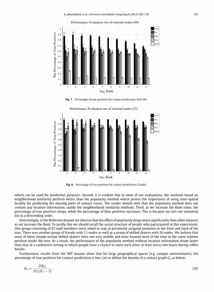
K. Jahanbakhsh et al. / Pervasive and Mobile Computing 8 (2012) 698–716 707
log2 Rank
Performance Evaluation (no of external nodes=60)
Fig. 7. Percentage of true positives for contact predictions (Info 06).
Fig. 8. Percentage of true positives for contact predictions (Camb).
which can be used for prediction purposes. Second, it is evident that in most of our evaluations, the methods based onneighborhood similarity perform better than the popularity method which proves the importance of using time-spatiallocality for predicting the missing parts of contact traces. The reader should note that the popularity method does notcontain any location information, unlike the neighborhood similarity methods. Third, as we increase the Rank value, thepercentage of true positives drops, while the percentage of false positives increases. This is because we sort our similaritylist in a descending order.
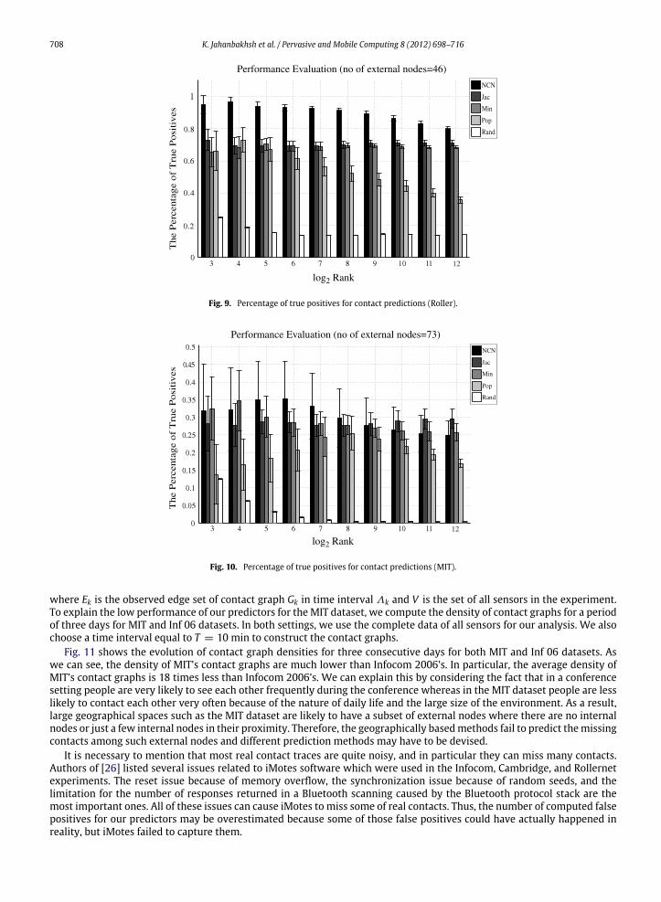
Interestingly, in the Rollernet datasetwe observe that the effect of popularity dropsmore significantly than other datasetsas we increase the Rank. To justify this we should recall the social structure of people who participated in this experiment.One group consisting of 25 staff members were asked to stay at previously assigned positions in the front and back of thetour. There was another group of friends with 11 nodes as well as a group of skilled skaters with 26 nodes. We believe thatmost of these people except skilled skaters were not very mobile and were located most of the time in the same relativeposition inside the tour. As a result, the performance of the popularity method without location information drops fasterthan that of a conference setting in which people have a chance to meet each other at least every two hours during coffeebreaks.
Furthermore, results from the MIT dataset show that for large geographical spaces (e.g. campus environments) thepercentage of true positives for contact predictions is low. Let us define the density of a contact graph Gk as below:
Dk =2|Ek|
|V |(|V | − 1), (10)
708 K. Jahanbakhsh et al. / Pervasive and Mobile Computing 8 (2012) 698–716
log2 Rank
Performance Evaluation (no of external nodes=46)
Fig. 9. Percentage of true positives for contact predictions (Roller).
Performance Evaluation (no of external nodes=73)
log2 Rank12
Fig. 10. Percentage of true positives for contact predictions (MIT).
where Ek is the observed edge set of contact graph Gk in time interval Λk and V is the set of all sensors in the experiment.To explain the low performance of our predictors for the MIT dataset, we compute the density of contact graphs for a periodof three days for MIT and Inf 06 datasets. In both settings, we use the complete data of all sensors for our analysis. We alsochoose a time interval equal to T = 10 min to construct the contact graphs.
Fig. 11 shows the evolution of contact graph densities for three consecutive days for both MIT and Inf 06 datasets. Aswe can see, the density of MIT’s contact graphs are much lower than Infocom 2006’s. In particular, the average density ofMIT’s contact graphs is 18 times less than Infocom 2006’s. We can explain this by considering the fact that in a conferencesetting people are very likely to see each other frequently during the conference whereas in the MIT dataset people are lesslikely to contact each other very often because of the nature of daily life and the large size of the environment. As a result,large geographical spaces such as the MIT dataset are likely to have a subset of external nodes where there are no internalnodes or just a few internal nodes in their proximity. Therefore, the geographically basedmethods fail to predict themissingcontacts among such external nodes and different prediction methods may have to be devised.
It is necessary to mention that most real contact traces are quite noisy, and in particular they can miss many contacts.Authors of [26] listed several issues related to iMotes software which were used in the Infocom, Cambridge, and Rollernetexperiments. The reset issue because of memory overflow, the synchronization issue because of random seeds, and thelimitation for the number of responses returned in a Bluetooth scanning caused by the Bluetooth protocol stack are themost important ones. All of these issues can cause iMotes to miss some of real contacts. Thus, the number of computed falsepositives for our predictors may be overestimated because some of those false positives could have actually happened inreality, but iMotes failed to capture them.

K. Jahanbakhsh et al. / Pervasive and Mobile Computing 8 (2012) 698–716 709
dens
ityde
nsity
Time
Time
Fig. 11. Evolution of contact graph densities for MIT and Inf 06 datasets.
Performance Evaluation (no of external nodes=79)
log2 Rank
Fig. 12. Percentage of true positives for contact predictions using social data (Info 06).
5.5. Contact prediction using offline social information
As we have mentioned earlier, Infocom 2006 data also includes participants’ social profiles. In this part of our analysiswe assume that we do not know anything about the contact trace except the social profiles of participants. In other words,we assume that all internal nodes act as surrogates of the external nodes. For testing our social methods, we compute socialsimilarities between all possible pairs of surrogates (e.g. (u, v, sim(u, v))) by using Eqs. (5) and (7) independently. We storethe computed Jacard and Foci similarities in Ljacsim and Lfocsim lists, respectively.We sort both of these similarity lists in descendingorder. These two lists are our social predictor results for Jacard and Foci similarities. To validate a prediction based on socialsimilarity such as (u, v, sim(u, v)), we randomly select a time intervalΛk as the time stepwhen a contact happened betweennodes u and v. For evaluation, we choose the first Rank number of predictions from our sorted similarity lists and inspectthem by using Infocom 2006’s contact trace data.
Fig. 12 shows the percentages of true positives regarding our prediction results when we only use social profiles. Thefigure shows that Foci similarity better reflects the similarity among people who attend a conference than Jacard does. FromFig. 12, we can make the interesting observation that using social data without any time and proximity information is stillhelpful for predicting missing contacts. The reader should note that the collected social profiles were only partial in thatsome people did not report their complete profiles, or any at all. By testing the distribution of social profiles, we have found

710 K. Jahanbakhsh et al. / Pervasive and Mobile Computing 8 (2012) 698–716
Fig. 13. Contact probability as a function of social and proximity information (Info 06).
that there are only around 100 pairs of nodeswhich are socially very similar (e.g. simsocfoc >= 0.2) while themajority of nodes
are not. Therefore, we expect that for log2 Rank values greater than 7, social profiles lose their effect for the prediction task.For the rest of our analysis we only use the Focus method to measure the social similarity between nodes.
We have already seen that the NCN method outperforms others as it contains the proximity information. Now, thequestion is if we can propose a better predictor by using both social profiles and NCN information. One could make thecase that once two users are in relative proximity (e.g. in the same room), the probability of meeting each other is high ifthey are also friends. To characterize the effects of social focus and NCN on contact probability, we select 75% of internalnodes as surrogates and repeat our evaluations as before by computing NCN scores between surrogates. We filter thosequadruples that have exactly c nodes in common (e.g. simk
ncn(., .) = c) and store all of them in the Lcsim list. Next, we use databinning to categorize all Lcsim’s quadruples into five equally sized intervals based on Foci similarity. We choose our intervalsas thrsoc ≤ simsoc
foc (u, v) ≤ thrsoc +0.1where thrsoc ∈ {0.0, 0.1, 0.2, 0.3, 0.4}. We then compute the percentage of surrogatesthat actually met each other. This gives us the contact probabilities for different social similarity and NCN values. We needto repeat the same process for all possible NCN values (e.g. 1 ≤ c ≤ 5).
Fig. 13 shows the contact probability among surrogates as a function of NCN and Foci similarity. We observe that forNCN values of 1, 2 and 3, as Foci similarity between two given nodes increases, the contact probability also becomes greater.Fig. 13 also shows that we cannot expect any improvement by adding social information when NCN is large. This is becausefor these cases the NCN acts as a dominant factor in contact probability. Our results are very encouraging as they provideincentive to incorporate social information with the NCN method to achieve a better performance.
One possible way for combining social information with NCN would be to compute prediction quadruples by using theNCN method. We then sort all quadruples in a descending order based on their NCN scores. Next, we use the social Focisimilarity as the second dimension to rank all quadruples with the same NCN scores in a descending order. This secondranking would give a higher weight to those pairs that are socially closer. This two-fold sorting would provide betterperformance than whenwe use only one of NCN or Foci similarity. Incorporating nodes’ contact rates with NCN informationwith a similar approach would also enhance the performance of the NCN predictor. We plan to pursue this direction asfuture work.
5.6. Statistical analysis of contact predictors
In the previous subsections, we analyzed our predictors with respect to true/false positives (i.e., what percentage ofpredicted contacts actually happened). However, an analysis of true/false negatives (i.e., what percentage of contacts thatactually happened we are able to predict) is missing. In this subsection, we compute several statistical measures in orderto give a better account of the performance of our predictors. To take into account both TP/FP and TN/FN, we compute fivestatistical measures including the true positive rate (TPR =
TPTP+FN ), the false positive rate (FPR =
FPFP+TN ), the precision
(precision =TP
TP+FP ), the accuracy (accuracy =TP+TNP+N ), and the root mean square error (RMSE) for our predictors.
For each statistical measure, we determine the missing contacts among the external surrogates as our observations.We also compute prediction results for each method in a similar manner as we did in the previous subsection. Havingobservations and prediction results, we can compute the first four statistical measures for different Rank values. We alsoemploy the RMSE to measure the difference between values predicted by our predictors and values actually observed fromthe real data. The RMSE analysis besides the other four statistical measures better illuminates the relative performanceof different predictors. Our ultimate goal is to better understand the predictor’s performances by computing the abovestatistical measures while changing the Rank value.

K. Jahanbakhsh et al. / Pervasive and Mobile Computing 8 (2012) 698–716 711
Performance Evaluation (no of external nodes=60)
log2 Rank
Fig. 14. True positive rates of NCN, Jacard, Min, Foci-NCN, and Popularity predictors (Infocom 06).
For our statistical analysis, we focus on the contacts during the first day of the Infocom 2006 conference from 11:00 AMto 2:00 PM. This three hours period covers different types of events in the conference. We only use three hours of Infocomdata because we want to limit the number of missing contacts as well as the Rank value. We randomly choose 75% of nodesand label them as external surrogates. We repeat our experiment 20 times and report the average results with their 95%confidence intervals. In the Infocom 2006 dataset, we found that on the average there are around 7k edges among externalsurrogates when we randomly select 75% of nodes as external surrogates. Thus, we have 3 ≤ log(Rank) ≤ ⌈log 7k⌉ = 13.
After removing edges between external surrogates, we construct all partial Gk’s where kmin ≤ k ≤ kmax. We also chooseτ = 240 s as the time interval. Let V obs
i denote the observation vector for ith run (1 ≤ i ≤ 20) in which we store observededges from the real data. Thus, for each external node pair (u, v) and kmin ≤ k ≤ kmax, we set V obs
i (u, v, k) = 1 if we observean undirected edge between those external nodes at kth time interval; otherwise, V obs
i (u, v, k) = 0. We also present ourprediction results with vector V pred
r,i for the ith run when Rank = r . In particular, V predr,i (u, v, k) = 1 if we find the quadruple
(u, v, k, sim(u, v)) in the first r number of predictions in the sorted similarity list; otherwise, V predr,i (u, v, k) = 0.
Having partial Gk’s, we generate the corresponding similarity list Lsim and sort it in a descending order for all predictionmethods in each run. Next, we store the first r number of predictions from the Lsim list in the V pred
i,r vector for post-processingsteps. By having observation vectors and prediction vectors for each Rank value, we compute the average of TPR, FPR,accuracy, and precision along with their 95% confidence intervals. Let |Vext | denote the number of external surrogates inour experiment. Let us also denote the set of all time intervals for our three hour analysis with Λ = {k|kmin ≤ k ≤ kmax}. ForRank = r and the ith run, we compute the RMSE of V pred
r,i with respect to the observation vector V obsi as shown in Eq. (11):
RMSE(V predr,i , V obs
i ) =
(u,v,k)∈Vext×Vext×Λ
(V predr,i (u, v, k) − V obs
i (u, v, k))|Vext |2
2
. (11)
Using Eq. (11), for each Rank value we compute the average of RMSE for all 20 runs and their 95% confidence intervals.Motivated by our results from Section 5.5, we also integrate the Foci similarity with the NCN predictor. We employ a two-fold sorting strategy by which we first sort prediction quadruples by using their NCNmeasures in a descending order. Next,we employ the social Foci similarity to sort all quadruples with the same NCN scores based on their social similarity in adescending order. We call this new predictor the Foci-NCN method.
Fig. 14 shows the TPR results for NCN, Jacard, Min, Foci-NCN, and Popularity methods. For small Rank values, the TPRsare low for all methods. We can also see that for small Rank values NCN and Foci-NCN perform slightly better than othermethods; however, the difference between the performance of methods based on the neighborhood similarity becomesnegligible for large Rank values. Furthermore, the Popularity method always performs worse than other methods whichmatch our results from Section 5.4. Fig. 15 presents our FPR results for all five methods. Here we observe the same patternas TPR results. Although the methods based on the neighborhood similarity perform very comparably for different Rankvalues, the Popularity method shows the worst FPR results.
Our precision results are presented in Fig. 16. As we can see, combining the social information with the NCNsimilarity in the Foci-NCN method obtains better precision results compared to other methods. This is in agreementwith our results from the previous subsection. However, when we increase the Rank value to predict more missingcontacts, the prediction methods based on the neighborhood similarity loose their predictive power and demonstrate

712 K. Jahanbakhsh et al. / Pervasive and Mobile Computing 8 (2012) 698–716
Performance Evaluation (no of external nodes=60)
log2 Rank
Fig. 15. False positive rates of NCN, Jacard, Min, Foci-NCN, and Popularity predictors (Infocom 06).
Performance Evaluation (no of external nodes=60)
log2 Rank
Prec
isio
n
Fig. 16. Precisions of NCN, Jacard, Min, Foci-NCN, and Popularity predictors (Infocom 06).
similar performance. Furthermore, we observe that the Popularity method demonstrates the poorest precision results. Thisis again because unlike the methods based on the neighborhood similarity, the Popularity predictor does not contain anygeographical information.
From Fig. 17, we can see that the accuracy is always high. This is because contact graphs are usually sparse as was shownin Fig. 11. As a result, even if the predictors do not infer any contacts between any pairs of external nodes, we still obtaina high accuracy. Therefore, the accuracy is not a reliable measure for the contact prediction task. Finally, Fig. 18 shows theRMSE results for our five different predictors. When we increase the Rank number, we achieve smaller RMSE values. Wealso observe that the Popularity method demonstrates the worst RMSE results.
In summary, if we focus onmoderate Rank values (e.g. Rank ≤ 10) where our predictors have not yet lost their predictivepower, we observe that the NCN and Foci-NCN methods outperform other three methods in terms of different statisticalmeasures. Furthermore, the Jacard and Min methods rank third and fourth while the Popularity method demonstrates thepoorest statistical performance for Infocom 2006’s conference data.
5.7. NCN scalability
In previous subsections, we have shown that the NCN outperforms other predictors in different social settings. Ourperformance results were demonstrated for a particular ratio of external to total nodes (i.e. 75%). However, it is importantto show how the predictors’ accuracy changes over diverse values of external to total nodes ratio. Since NCN predictions arestatically more significant than other predictors, here we just show the scalability results for NCN predictors for Infocom2006 and Rollernet datasets. Figs. 19 and 20 demonstrate the scalability of the NCN predictor for Infocom 2006 and Rollernetsettings respectively. As we can see, the ratio of external nodes to total nodes has been changed from 20% to 80%.

K. Jahanbakhsh et al. / Pervasive and Mobile Computing 8 (2012) 698–716 713
Performance Evaluation (no of external nodes=60)
log2 Rank
Acc
urac
y
Fig. 17. Accuracies of NCN, Jacard, Min, Foci-NCN, and Popularity predictors (Infocom 06).
Performance Evaluation (no of external nodes=60)
log2 Rank
RM
SE
Fig. 18. RMSE of NCN, Jacard, Min, Foci-NCN, and Popularity predictors (Infocom 06).
log2 Rank
Fig. 19. Scalability results for NCN predictor (Info06).

714 K. Jahanbakhsh et al. / Pervasive and Mobile Computing 8 (2012) 698–716
Fig. 20. Scalability results for NCN predictor (Roller).
Fig. 21. Number of predictions for NCN predictor (Inf 06/Roller).
There are several observations worth noting from the scalability results. First, in both settings the predictor accuracydrops quickly when the ratio is 20%. This can be justified by considering the fact that in this case actually there are not manymissing edges to predict. This becomes clear if we compute the number of predictions for different ratio values as shownin Fig. 21. We can see that when the number of external nodes is just 20% of the total number of nodes, the total number ofpredictions produced by NCN is significantly less than 4096 for both datasets. However, as we increase the ratio of externalto total nodes, there are more missing edges that NCN can predict. Finally, our scalability results also show that the NCNpredictor performs well when we increase the percentage of external nodes. In other words, when the number of externalnodes increases, there are many missing edges in contact graphs that can be inferred by the NCN predictor successfully.
6. Why does NCN perform well?
In Section 5.4, we have seen that as we increase the number of predictions, the performances of our predictors drop.This is because when we increase the number of predictions, the similarity scores such as NCN drop. Fig. 22 shows therelation between the probability of a contact between two external nodes’ surrogates and their NCN value for differentnumbers of external nodes. As we can see, the NCN score and the contact probability are positively correlated. In otherwords, decreasing the NCN score decreases the contact probability. This explains why increasing the number of predictionsreduces the performances of our predictors. According to Fig. 22, as soon as two external nodes’ surrogates have even onenode in common, their meeting chance increases by a factor of four which is quite significant. Fig. 22 also shows that as theNCN increases, the performance of prediction also improves.
Our performance results clearly show that the number of common neighbors more accurately predicts the missingcontacts among external nodes than other predictors. In this section we try to explain the performance of the number

K. Jahanbakhsh et al. / Pervasive and Mobile Computing 8 (2012) 698–716 715
Fig. 22. Probability of contact as a function of NCN for Infocom06 dataset.
of common neighbors. As mentioned earlier, we expect spatial locality to increase the meeting probability between nodes.Thus, we need to estimate the distances between nodes by using a metric. Suppose two nodes u and v with similar radiusrange r are located at a distance d fromeach other. If these twonodes have at least one commonneighbor, i.e. a node iswithintheir communication range, we can infer that the intersection area between their circles is greater than zero as shown inFig. 3. This requires an upper bound equal to 2× r for the distance between nodes u and v (i.e. d(u, v) < 2× r). If we assumea uniform distribution for nodes’ locations on the plane, we can explain the success of the NCN.
Let us assume that we have n nodes with radius range r which are uniformly distributed in a region with an area A (e.g. aconference room). In this graph, there is an edge between two nodes u and v if their distance is less than r (i.e. d(u, v) < r).The resulting graph is a random geometric graph (RGG) [27]. Researchers have used RGGs to model the wireless ad-hocnetworks [28]. A direct consequence of the dependency of links on the geometric distance between nodes is that there is anincreased probability of two nodes being connectedwith each other if they have a common neighbor.We have also observedthis increasing pattern in our contact probability graph (Fig. 22). Let Ei denote the event of an occurrence of edge ei in thedescribed RGG. The probability of occurrence of an edge ei between a pair of nodes is Pr(Ei) =
πr2|A|
. For two distinct edges
ei = (u, v) and ej = (u, w), we have Pr(EiEj) = Pr(Ei)Pr(Ej) = (πr2|A|
)2. For three distinct edges ei = (u, v), ej = (u, w), andek = (v, w), the authors of [29] derived the probability that these three edges form a triangle as follows:
Pr(EiEjEk) =
π −
3√3
4
πr4
|A|2. (12)
Using Eq. (12), we derive the probability for occurrence of edge ei between nodes u and v given they have one commonneighbor (node w) as follows:
Pr(Ei|EjEk) =Pr(EiEjEk)Pr(EjEk)
=π −
3√3
4
π. (13)
Eq. (13) gives Pr(Ei|EjEk) ≈ 0.58 which is obviously more significant than the small value of Pr(Ei) =πr2|A|
(|A| ≫ πr2)which again justifies our observation in Fig. 22 where the probability of contact suddenly jumps as soon as nodes haveone common neighbor. Unfortunately computing the link probability when the number of common neighbors is greaterthan one becomes much harder. This is mainly because of the dependency issues that the third and fourth edges add to theconditional probability formulation.
7. Conclusions and future work
In this paper, we have studied the problem of contact prediction in the context of mobile social networks. We havedescribed different methods for predicting missing contacts. We have examined our methods by using real contact tracescollected from different social settings. Our results show that time-spatial based scores provide the most reliable resultsfor predicting missing contacts among external nodes. We have also studied the power of social profiles to predict humanmobility. We have shown that combining social information with time-spatial information provides better performanceresults than using each of them independently. We believe that our contributions have significant practical values becausethey allow researchers to study properties of large scale contact graphs by sampling only a portion of the original graphs.

716 K. Jahanbakhsh et al. / Pervasive and Mobile Computing 8 (2012) 698–716
Our results are also important for mobility modeling since they explain how people move in different social settings suchas conference and campus environments.
For our future work, we plan to propose more efficient methods for predicting missing contacts in large geographicalspaces as in theMIT dataset. In Section 6,wehave assumed that nodes are uniformly distributed on the plane; however,morerealistically one should expect nodes’ locations to be influenced by social characteristics of people. Thus, we can introducea Geometric Social Network model (GSN) instead of RGG. Characterizing nodes’ distribution in the GSN model is anotherinteresting open problem that we would like to study in the future.
References
[1] N. Eagle, A. Pentland, D. Lazer, Inferring social network structure using mobile phone data, Proceedings of the National Academy of Sciences (PNAS)106 (36) (2009) 15274–15278.
[2] A. Chaintreau, P. Hui, J. Scott, R. Gass, J. Crowcroft, C. Diot, Impact of human mobility on opportunistic forwarding algorithms, IEEE Transactions onMobile Computing 6 (6) (2007) 606–620.
[3] P.U. Tournoux, J. Leguay, F. Benbadis, V. Conan, M. Dias de Amorim, J. Whitbeck, The accordion phenomenon: analysis, characterization, and impacton DTN routing, in: IEEE INFOCOM 2009 — The 28th Conference on Computer Communications, IEEE, 2009, pp. 1116–1124.
[4] M. Musolesi, C. Mascolo, A community based mobility model for ad hoc network research, in: Proceedings of the 2nd International Workshop onMulti-hop ad hoc Networks, REALMAN’06, ACM, New York, NY, USA, 2006, pp. 31–38.
[5] W.-J. Hsu, T. Spyropoulos, K. Psounis, A. Helmy, Modeling spatial and temporal dependencies of user mobility in wireless mobile networks, IEEE/ACMTransactions on Networking 17 (5) (2009) 1564–1577.
[6] E.M. Daly, M. Haahr, Social network analysis for routing in disconnected delay-tolerant magnets, in: Proceedings of the 8th ACM InternationalSymposium on Mobile ad hoc Networking and Computing, ACM, New York, NY, USA, 2007, pp. 32–40.
[7] P. Hui, J. Crowcroft, E. Yoneki, Bubble rap: social-based forwarding in delay tolerant networks, in: Proceedings of the 9thACM International Symposiumon Mobile ad hoc Networking and Computing, ACM, New York, NY, USA, 2008, pp. 241–250.
[8] K. Jahanbakhsh, G.C. Shoja, V. King, Social-greedy: a socially-based greedy routing algorithm for delay tolerant networks, in:MobiOpp’10: Proceedingsof the Second International Workshop on Mobile Opportunistic Networking, ACM, New York, NY, USA, 2010, pp. 159–162.
[9] J. Leguay, A. Lindgren, J. Scott, T. Friedman, J. Crowcroft, Opportunistic content distribution in an urban setting, in: Proceedings of the 2006 SIGCOMMWorkshop on Challenged Networks, CHANTS’06, ACM, New York, NY, USA, 2006, pp. 205–212.
[10] A. Mtibaa, A. Chaintreau, J. LeBrun, E. Oliver, A.-K. Pietilainen, C. Diot, Are you moved by your social network application? in: Proceedings of the FirstWorkshop on Online Social Networks, WOSN’08, ACM, New York, NY, USA, 2008, pp. 67–72.
[11] D. Liben-Nowell, J. Kleinberg, The link prediction problem for social networks, in: CIKM’03: Proceedings of the Twelfth International Conference onInformation and Knowledge Management, ACM, New York, NY, USA, 2003, pp. 556–559.
[12] D.S. Goldberg, F.P. Roth, Assessing experimentally derived interactions in a small world, Proceedings of the National Academy of Sciences (PNAS) 100(8) (2003) 4372–4376.
[13] V. Sivaraman, S. Grover, A. Kurusingal, A. Dhamdhere, A. Burdett, Experimental study of mobility in the soccer field with application to real-timeathletemonitoring, in:Wireless andMobile Computing, Networking and Communications (WiMob), 2010 IEEE 6th International Conference on, 2010,pp. 337–345.
[14] T. Hossmann, T. Spyropoulos, F. Legendre, Know thy neighbor: Towards optimal mapping of contacts to social graphs for DTN routing, in: Proceedingsof IEEE INFOCOM 2010, IEEE, 2010, pp. 1–9.
[15] D. Liben-Nowell, J. Kleinberg, The link-prediction problem for social networks, Journal of the American Society for Information Science and Technology58 (2007) 1019–1031.
[16] M.A. Hasan, V. Chaoji, S. Salem, M. Zaki, Link prediction using supervised learning, in: In Proc. of SDM 06workshop on Link Analysis, Counterterrorismand Security, 2006.
[17] J. Leskovec, D. Huttenlocher, J. Kleinberg, Predicting positive and negative links in online social networks, in: Proceedings of the 19th InternationalConference on World Wide Web, WWW’10, ACM, New York, NY, USA, 2010, pp. 641–650.
[18] K. Jahanbakhsh, G.C. Shoja, V. King, Predicting human contacts in mobile social networks using supervised learning, in: Proceedings of the FourthAnnual Workshop on Simplifying Complex Networks for Practitioners, SIMPLEX ’12, ACM, New York, NY, USA, 2012, pp. 37–42.
[19] K. Jahanbakhsh, G.C. Shoja, V. King, Predicting missing contacts in mobile social networks, in: World of Wireless Mobile and Multimedia Networks,IEEE, 2011, pp. 1–9.
[20] D.J. Watts, S.H. Strogatz, Collective dynamics of ‘small-world’ networks, Nature 393 (6684) (1998) 440–442.[21] P. Jaccard, Étude comparative de la distribution florale dans une portion des alpes et des jura, Bulletin del la Société Vaudoise des Sciences, Naturelles
37 (1901) 547–579.[22] M. McPherson, L. Smith-Lovin, J.M. Cook, Birds of a feather: homophily in social networks, Annual Review of Sociology 27 (1) (2001) 415–444.[23] J. Kleinberg, Small-world phenomena and the dynamics of information, in: In Advances in Neural Information Processing Systems (NIPS) 14, MIT
Press, 2001, p. 2001.[24] A.L. Barabasi, R. Albert, Emergence of scaling in random networks, Science (New York, N.Y.) 286 (5439) (1999) 509–512.[25] P. Hui, J. Crowcroft, How small labels create big improvements, in: Proceedings of the Fifth IEEE International Conference on Pervasive Computing
and Communications Workshops, PERCOMW’07, IEEE Computer Society, Washington, DC, USA, 2007, pp. 65–70.[26] E. Nordström, C. Diot, R. Gass, P. Gunningberg, Experiences from measuring human mobility using bluetooth inquiring devices, in: MobiEval’07:
Proceedings of the 1st International Workshop on System Evaluation for Mobile Platforms, ACM, New York, NY, USA, 2007, pp. 15–20.[27] M. Penrose, Random Geometric Graphs, Oxford University Press, 2003.[28] P. Gupta, P.R. Kumar, Critical power for asymptotic connectivity in wireless networks, 1998, pp. 547–566.[29] C.W. Yu, Computing subgraph probability of random geometric graphs with applications in quantitative analysis of ad hoc networks, IEEE Journal on
Selected Areas in Communications 27 (7) (2009) 1056–1065.