predicting juvenile recidivism 1 running head:...
TRANSCRIPT

Predicting Juvenile Recidivism 1
Running head: PREDICTING JUVENILE RECIDIVISM USING LATENT GROWTH MODELING
Predicting Juvenile Recidivism
Using Latent Growth Modeling
Michael J Tanana
University of Utah

Predicting Juvenile Recidivism 2
Abstract
Although this study found evidence that the “age-crime” curve is not just a group phenomenon, but an
individual phenomenon, there was also evidence that this is not the ideal way to model delinquency for
all youth. Mixture modeling, using two groups, showed that many youth who offend are “one timers”
who offend once at any time during their adolescence (and every age is equally likely, contrary to
Moffit’s “adolescent limited” typology). The second group represents youth who offend more
frequently (about once a year at their peak) and increase up through age 16, then decrease. Latent
growth modeling, as used in this case, does not improve prediction of delinquency through adolescence
over more commonly used methods. Post-hoc analyses suggest that recidivism may best be modeled as
a residualized change score, predicted from the two prior time points to the one being estimated.

Predicting Juvenile Recidivism 3
Predicting Juvenile Recidivism
Using Latent Growth Modeling
Background
Developmental Anti-Social Behavior
It is well established in the developmental psychology literature that antisocial behavior (ASB) follows a
non-linear trajectory in adolescents and that early initiation of ASB is associated with increased severity
and persistence of this behavior later in life (Moffit, 1993). Unfortunately, this understanding has not
translated to an improvement in the way that juvenile risk assessments make use of offense history to
predict the likelihood of future delinquent involvement. The common practice of creating a simple
additive score to predict future recidivism essentially discards of potentially useful data: the age at each
offense.
Latent Growth Curve modeling (LGM) is a common technique that developmental psychologists have
used to look at juvenile delinquency over time. Most of these studies, however, have made use of self
and parent report questionnaires (Stoolmiller, 1994; Mason, 2001; Wiesner and Windle, 2004).
Common shortcomings of many of these developmental trajectory models of delinquency is they make
use of smaller time frames within the youths’ development . For example, Wiesner and Windle (2004)
only looked at ages from 15.5 to 17. No studies were identified that attempted to make use of LGM for
the purpose of predicting recidivism.

Predicting Juvenile Recidivism 4
Theoretical
This study posits that overt anti-social behavior is a latent trait underlying the observed variable of
delinquency, (operationalized as law breaking events). Moreover, it is assumed that this trait is
measured with a great deal of error. This underlying trait differs a great deal from individual to
individual, but has a similar shape across individuals. Presumably it accelerates in early adolescence and
then slows in late adolescence. It reaches a peak and then decreases in early, into late adulthood.
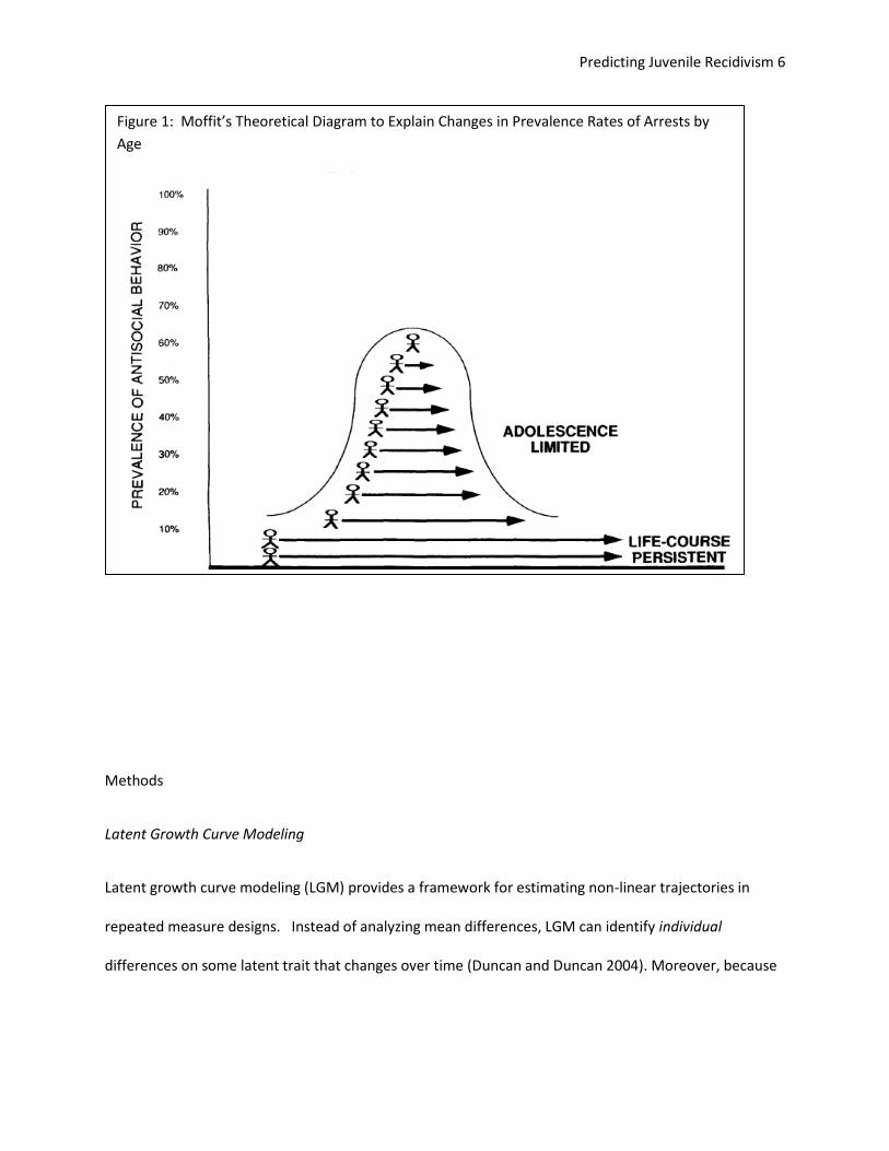
Essentially, it follows a bell curve that replicates Moffit’s (1993) curve of offenses by age (see figure 1).
Those who are “early starters” would also be “late finishers”, consistent with Moffit’s theory of life
course persistent vs. adolescent limited youth. Moffit argues that prevalence rates for arrests by age
that show a peak of activity around age 17 can be explained by new, adolescent limited offenders
joining the ranks of life course persistent offenders. She supports this claim using national statistics of
new offenders by age that shows a constant increase up to age 16 and then a sharp decrease. This
finding, though true, does not exclude the additional influence of increases in the number of offenses by
age as well.
Stolzenberg and D’Alessio (2008) break down the relationship between age and offense rate by gender,
ethnicity, type of crime, and solo vs. communal offending. They conclude the “age crime curve”, or the
parabolic curve that Moffit wrote about, is virtually unchanged within these subgroups. In other words,
the finding that delinquency increases through the teenage years and then decreases through early
adulthood is true for all ethnic subgroups and types of offenders examined in their research. This study,
unfortunately, cannot distinguish between increases in number of offenders or increases in number of
offenses per individual. Farrington (2005) writes that it is still contentious whether individual
frequency of offending peaks at late adolescence, or whether there is no relationship between age and

Predicting Juvenile Recidivism 5
frequency of offending. In investigating this phenomenon of rate of offending, many researchers (see
Loeber and Snyder, 1993) make a theoretical assumption that youth should be characterized as active
and non-active, and that offense rates should only be looked at during the youth’s active period.
This study hypothesizes that frequency of offending does peak in middle adolescence, and that offenses
early in life will confer risk of a higher frequency of offenses in late adolescence. But, in contrast to
many researchers, a single discrete ‘age at first arrest’ is not the most predictive measure. Instead,
recorded offending behavior is an observed measurement (with a great deal of measurement error) of a
latent trait, overt anti-social behavior, much of which is either not illegal or not observed by authorities.
This latent trait, as understood in this context, has a non-linear trajectory that peaks in late adolescence,
and for most youth, desists later in adulthood. Importantly, this theory predicts that the shape of this
curve is similar across individuals, but the height of the curve varies between individuals.
This theory would have several implications for prediction:
1. An offense earlier in life (between age 8 and 12) would confer greater risk for offenses later in
adolescence than an offense in mid-adolescence (13-15).
2. Predicting recidivism based on one year prior offenses, without assuming non-linear growth,
would result in a biased estimate for all youth: an underestimate for younger youth and an
overestimate for older youth.
3. Number of offenses at every age hold important information for approximating the latent curve
of delinquency. Using every age should reduce error in approximating delinquency. Using just
one (age at first arrest) would confer too much error to any model.
Predicting Juvenile Recidivism 6
Methods
Latent Growth Curve Modeling
Latent growth curve modeling (LGM) provides a framework for estimating non-linear trajectories in
repeated measure designs. Instead of analyzing mean differences, LGM can identify individual
differences on some latent trait that changes over time (Duncan and Duncan 2004). Moreover, because
Figure 1: Moffit’s Theoretical Diagram to Explain Changes in Prevalence Rates of Arrests by
Age

Predicting Juvenile Recidivism 7
it is a special case of structural equation modeling, it allows for testing of a growth model versus a
competing non-growth model as well as absolute tests of model fit.
McArdle and Nesselroade (2003) lay out the basic form of the latent growth curve model:
represents the intercept for person n and A*t+, the effect of the slope (γs) for person n ( ) on the
observation at each time t ( . In this study two of the A[t] paths will be fixed to scale the rate of
change, while the rest will be estimated to allow for non-linear growth. The null model, or no growth
model is:
The null model posits that scores at each time t are simply the function of the mean for person n )
and error. This null model is equivalent to a mean or sum score of the observations across times, or that
each subsequent score can best be estimated by taking the mean of the previous scores.
In its most general form, latent growth modeling assumes that there is a latent growth function (a line, a
curve or a parabola) that underlies observations for each individual. Each observation in time(Y[t]) for
each person is assumed to have measurement error, but to be a manifestation of that unobserved curve
or line. For a linear latent model, this latent line can be described by two parameters for each person:
the slope and the intercept. A multilevel model can now use this collection of slopes and intercepts as
two criterions that have the error of each individual observation removed.
Predicting Juvenile Recidivism 8
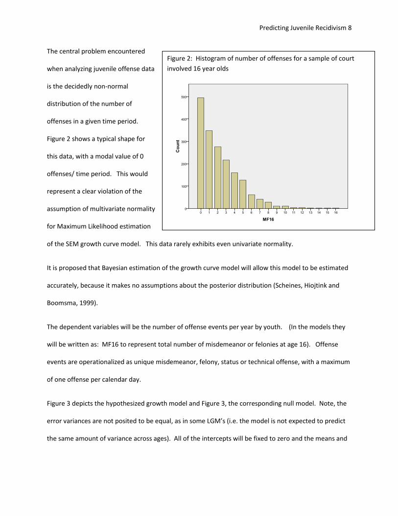
Figure 2: Histogram of number of offenses for a sample of court
involved 16 year olds
The central problem encountered
when analyzing juvenile offense data
is the decidedly non-normal
distribution of the number of
offenses in a given time period.
Figure 2 shows a typical shape for
this data, with a modal value of 0
offenses/ time period. This would
represent a clear violation of the
assumption of multivariate normality
for Maximum Likelihood estimation
of the SEM growth curve model. This data rarely exhibits even univariate normality.
It is proposed that Bayesian estimation of the growth curve model will allow this model to be estimated
accurately, because it makes no assumptions about the posterior distribution (Scheines, Hiojtink and
Boomsma, 1999).
The dependent variables will be the number of offense events per year by youth. (In the models they
will be written as: MF16 to represent total number of misdemeanor or felonies at age 16). Offense
events are operationalized as unique misdemeanor, felony, status or technical offense, with a maximum
of one offense per calendar day.
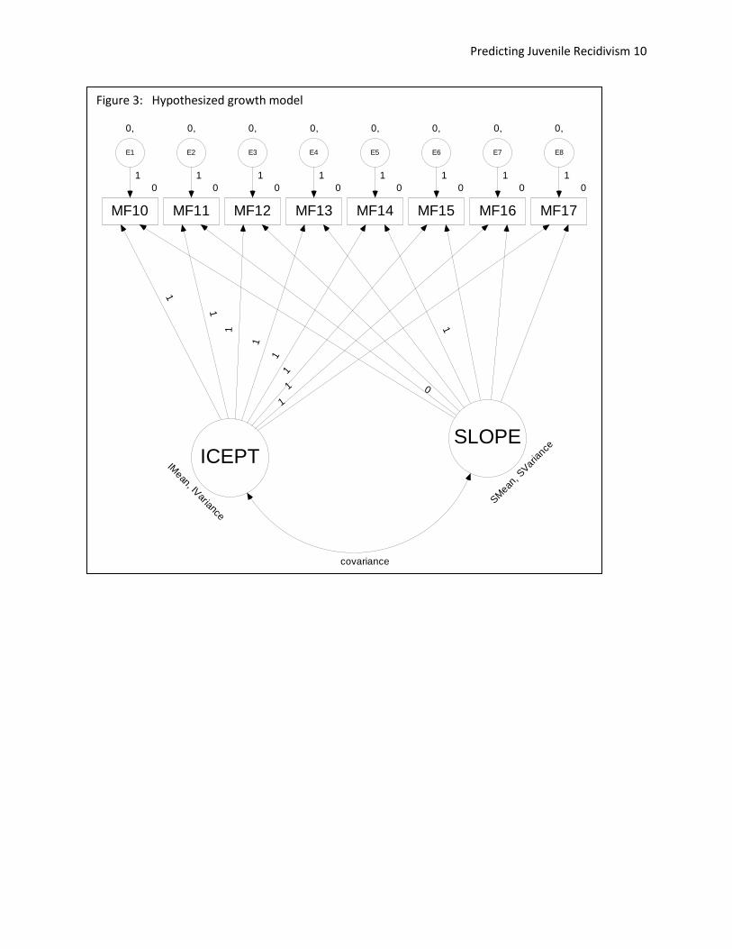
Figure 3 depicts the hypothesized growth model and Figure 3, the corresponding null model. Note, the
error variances are not posited to be equal, as in some LGM’s (i.e. the model is not expected to predict
the same amount of variance across ages). All of the intercepts will be fixed to zero and the means and

Predicting Juvenile Recidivism 9
variances of the slope and intercept will be estimated. The priors for the Bayesian estimation will all be
non-informative (uniform distribution).
Absolute goodness of fit will be calculated based on the posterior predictive p, and the relative
goodness of fit for competing models will be compared using the Deviance Information Criteria (DIC).
The DIC can be used for both nested and non-nested model comparison. Smaller values of the DIC
represent better fit than larger values, and models within 5 points on the DIC are considered not
different from one another (Lee, 2007). Bayesian estimation uses “credible intervals” in place of
confidence intervals. Whereas confidence intervals are based on assumptions about sampling
distributions, credible intervals are based on the obtained distributions of the parameter of interests
from repeated simulations of the model. For most models, 95% credible intervals will be presented.
These represent the bounds of the inner 95% of the parameter estimates.
Predicting Juvenile Recidivism 10
Figure 3: Hypothesized growth model
IMean, IV
ariance
ICEPT
SM
ean, S
Varia
nceSLOPE
0
MF10
1
0
0
MF11
1
0
MF121
0
MF13
1
0
MF14
1
1
0
MF15
1
0
MF16
1
0
MF17
1
0,
E1
1
0,
E2
1
0,
E3
1
0,
E4
1
0,
E5
1
0,
E6
1
0,
E7
1
0,
E8
1
covariance

Predicting Juvenile Recidivism 11
In addition to testing whether juvenile offenses are best modeled using a non-linear latent growth
model, the relationship of gender to offending will be tested. The hypothesis is that the shape of
growth will not differ between genders, but rather there will be mean differences in slopes and
intercepts between males and females. In other words, males and females will not differ on the
essential shape of the curve of offending, but rather on their intercepts and slopes of this curve. To test
this hypothesis, a multiple group analysis will be employed based on a procedure similar to testing for
measurement invariance across groups (McArdle & Nesselroade, 2003). Two competing stacked
Figure 4: No-growth null model.
IMean, IV
ariance
ICEPT
0
MF10
1
0
MF11
1
0
MF121
0
MF13
1
0
MF14
1
0
MF15
1
0
MF16
1
0
MF17
1
0,
E1
1
0,
E2
1
0,
E3
1
0,
E4
1
0,
E5
1
0,
E6
1
0,
E7
1
0,
E8
1

Predicting Juvenile Recidivism 12
models will be tested, one where the estimated paths of the slope on each age are fixed between
genders and one where they are free to vary. In other words, these models are testing whether
(for all estimated A[t])
If these two models do not differ significantly based on the Deviance Information Criteria, then it is then
appropriate to test whether the variance components of the slope and intercept are equivalent, with
the A[t] paths equated between groups. Again, two competing models, one with intercept and slope
variances equated and one where they are freely estimated between groups will be compared. Finally,
if these two models are not significantly different, then a final model can employed testing for mean
differences on the slope and intercept between groups. Following McArdle and Nesselroade (2003),
this can be tested without using a stacked model, but by a simple mixed effects model (see figure 4).
The unstandardized paths from “Sex” to the slope and intercept represent the mean differences
between males and females on each latent trait (with the intercept representing the mean of whichever
group is coded ‘0’).
This stacked model procedure has the advantage of testing both aspects of the hypothesis: whether
there exist structural differences between groups and whether there are mean differences between
groups.
Participants
All individuals with dates of birth between 1/1/1990 to 12/31/1991 and any felony, misdemeanor,
status or technical charge in the state court database were selected. This range was selected to collect
Predicting Juvenile Recidivism 13
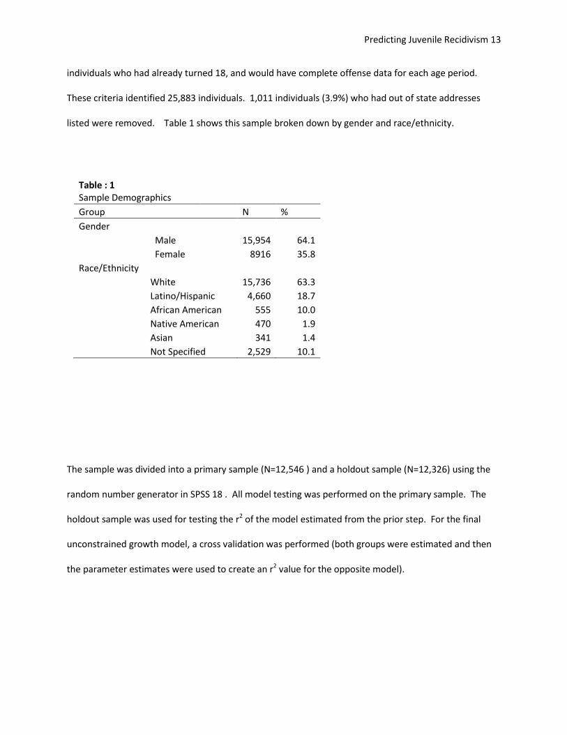
individuals who had already turned 18, and would have complete offense data for each age period.
These criteria identified 25,883 individuals. 1,011 individuals (3.9%) who had out of state addresses
listed were removed. Table 1 shows this sample broken down by gender and race/ethnicity.
The sample was divided into a primary sample (N=12,546 ) and a holdout sample (N=12,326) using the
random number generator in SPSS 18 . All model testing was performed on the primary sample. The
holdout sample was used for testing the r2 of the model estimated from the prior step. For the final
unconstrained growth model, a cross validation was performed (both groups were estimated and then
the parameter estimates were used to create an r2 value for the opposite model).
Table : 1 Sample Demographics
Group N %
Gender Male 15,954 64.1
Female 8916 35.8
Race/Ethnicity White 15,736 63.3
Latino/Hispanic 4,660 18.7
African American 555 10.0
Native American 470 1.9
Asian 341 1.4
Not Specified 2,529 10.1

Predicting Juvenile Recidivism 14
Missing Data
Because the selection criteria identified only individuals who had turned 18 and had only lived in Utah,
there was no missing data for number of offenses at each age. 36 individuals (.1%) were missing
Race/Ethnicity data and 2 individuals (less than .1%) were missing gender data. For any analyses that
included these variables, Bayesian imputation was performed concurrently with the analysis (in AMOS
17).

Predicting Juvenile Recidivism 15
Results
Intercept Only Model
The intercept only model posited that a juvenile’s offending over time can be modeled by just their own
average number of offenses per year. At level one:
As in all models run, the error variances were heterogeneous.
Table 2 shows the Bayesian estimation of the intercept only model. For this model, the mean intercept
across individuals was .04 and was significantly different from zero based on the 95% Bayesian credible
intervals. This predicts that the average offending across individuals is .04 offenses per year. The
variance of the intercept ( σ2= .008), also significantly differed from zero indicating that the average
offending varied significantly across individuals.
Table 2 Bayesian Unstandardized Estimates: Intercept Only
Model Predicting Number of Offenses at Each Age
Parameter Mean 95% Lower
95% Upper
Means Intercept 0.047* 0.044 0.049
Variances Intercept 0.008* 0.008 0.009
DIC=18,732 ; ppp=.00
*95% Credible Interval did not include zero
Predicting Juvenile Recidivism 16
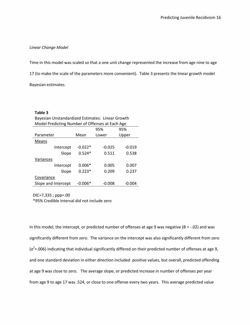
Linear Change Model
Time in this model was scaled so that a one unit change represented the increase from age nine to age
17 (to make the scale of the parameters more convenient). Table 3 presents the linear growth model
Bayesian estimates.
In this model, the intercept, or predicted number of offenses at age 9 was negative (B = -.02) and was
significantly different from zero. The variance on the intercept was also significantly different from zero
(σ2=.006) indicating that individual significantly differed on their predicted number of offenses at age 9,
and one standard deviation in either direction included positive values, but overall, predicted offending
at age 9 was close to zero. The average slope, or predicted increase in number of offenses per year
from age 9 to age 17 was .524, or close to one offense every two years. This average predicted value
Table 3 Bayesian Unstandardized Estimates: Linear Growth
Model Predicting Number of Offenses at Each Age
Parameter Mean 95% Lower
95% Upper
Means Intercept -0.022* -0.025 -0.019
Slope 0.524* 0.511 0.538
Variances Intercept 0.006* 0.005 0.007
Slope 0.223* 0.209 0.237
Covariance Slope and Intercept -0.006* -0.008 -0.004
DIC=7,335 ; ppp=.00 *95% Credible Interval did not include zero

Predicting Juvenile Recidivism 17
was significantly different from zero. The variance on the slope was also significantly different from zero
(σ2=.223) and was larger than the variance on the intercept. This indicates that individuals varied more
on their change over time than they did on their predicted levels of offending at age 9. This model
predicts that the middle two standard deviations of individual slopes in this sample would range from
.06 to 1.006, or increases close to zero and others close to one offense per year. The covariance
between the slope and the intercept was -.006 and was significantly different from zero, indicating that
higher predicted offending at age 9 actually predicted more modest increases in offending over the
course of adolescence.
The absolute model fit of the linear model was not adequate, but the relative model fit improved over
the no growth model (The DIC decreased from 18,732 to 7,335). The negative predicted values of
offending at age 9 also suggest that a linear model is not an acceptable one for this data.
Predicting Juvenile Recidivism 18
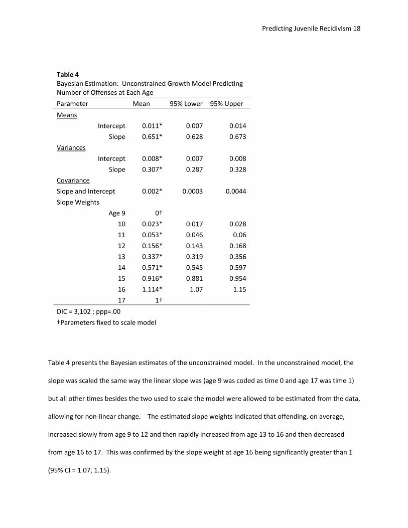
Table 4 presents the Bayesian estimates of the unconstrained model. In the unconstrained model, the
slope was scaled the same way the linear slope was (age 9 was coded as time 0 and age 17 was time 1)
but all other times besides the two used to scale the model were allowed to be estimated from the data,
allowing for non-linear change. The estimated slope weights indicated that offending, on average,
increased slowly from age 9 to 12 and then rapidly increased from age 13 to 16 and then decreased
from age 16 to 17. This was confirmed by the slope weight at age 16 being significantly greater than 1
(95% CI = 1.07, 1.15).
Table 4 Bayesian Estimation: Unconstrained Growth Model Predicting
Number of Offenses at Each Age
Parameter Mean 95% Lower 95% Upper
Means Intercept 0.011* 0.007 0.014
Slope 0.651* 0.628 0.673
Variances Intercept 0.008* 0.007 0.008
Slope 0.307* 0.287 0.328
Covariance Slope and Intercept 0.002* 0.0003 0.0044
Slope Weights Age 9 0†
10 0.023* 0.017 0.028
11 0.053* 0.046 0.06
12 0.156* 0.143 0.168
13 0.337* 0.319 0.356
14 0.571* 0.545 0.597
15 0.916* 0.881 0.954
16 1.114* 1.07 1.15
17 1†
DIC = 3,102 ; ppp=.00 †Parameters fixed to scale model

Predicting Juvenile Recidivism 19
In this model, the predicted offending at age 9 was positive and significantly different from zero (B =
.011). The intercept variance was also significantly different from zero, suggesting that individuals
varied on predicted offending at age 9. The average slope, or predicted increase in offending from age
9 to age 17, was .651 and was significantly different from zero. Because the weight at age 16 went
above 1, this would predict individuals, on average, increase to .725 offenses per year above the
intercept before decreasing to .651. The variance on the slope (σ2=.307) was also significantly different
from zero, indicating that individuals varied on change in offending over time. Figure 3 presents plots
of the unconstrained model at the mean slope and intercept, with additional plots one standard
deviation above and one standard deviation below the mean slope.
This model was also not adequate by the measure of absolute fit (ppp=.00) but was an improvement
from the linear model (Reduction in DIC = 4,233).
Predicting Juvenile Recidivism 20
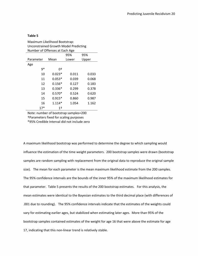
A maximum likelihood bootstrap was performed to determine the degree to which sampling would
influence the estimation of the time weight parameters. 200 bootstrap samples were drawn (bootstrap
samples are random sampling with replacement from the original data to reproduce the original sample
size). The mean for each parameter is the mean maximum likelihood estimate from the 200 samples.
The 95% confidence intervals are the bounds of the inner 95% of the maximum likelihood estimates for
that parameter. Table 5 presents the results of the 200 bootstrap estimates. For this analysis, the
mean estimates were identical to the Bayesian estimates to the third decimal place (with differences of
.001 due to rounding). The 95% confidence intervals indicate that the estimates of the weights could
vary for estimating earlier ages, but stabilized when estimating later ages. More than 95% of the
bootstrap samples contained estimates of the weight for age 16 that were above the estimate for age
17, indicating that this non-linear trend is relatively stable.
Table 5 Maximum Likelihood Bootstrap:
Unconstrained Growth Model Predicting Number of Offenses at Each Age
Parameter Mean 95% Lower
95% Upper
Age 9* 0†
10 0.023* 0.011 0.033
11 0.053* 0.039 0.068
12 0.156* 0.127 0.183
13 0.336* 0.299 0.378
14 0.570* 0.524 0.620
15 0.915* 0.860 0.987
16 1.114* 1.054 1.162
17* 1†
Note: number of bootstrap samples=200 †Parameters fixed for scaling purposes *95% Credible Interval did not include zero
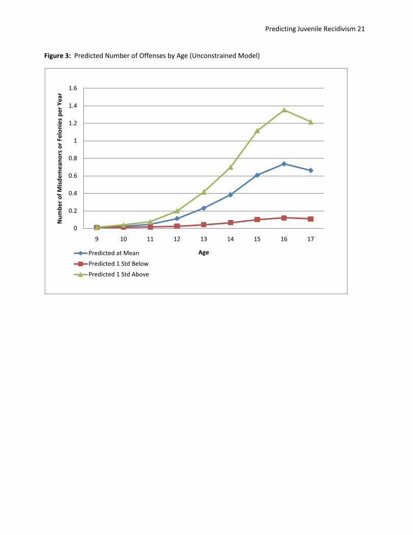
Predicting Juvenile Recidivism 21
Figure 3: Predicted Number of Offenses by Age (Unconstrained Model)
0
0.2
0.4
0.6
0.8
1
1.2
1.4
1.6
9 10 11 12 13 14 15 16 17
Nu
mb
er
of
Mis
de
me
ano
rs o
r Fe
lon
ies
pe
r Y
ear
AgePredicted at Mean
Predicted 1 Std Below
Predicted 1 Std Above

Predicting Juvenile Recidivism 22
For the quadratic model, time was coded 0 at age 9 and 8 at age 17. In this model the mean intercept
and quadratic coefficients differed from zero, but not the slope (B=.001, 95% CI: -.002, .004). This would
indicate that a large portion of the linear main effect from the previous models can be described with a
quadratic term. The intercept, slope and quadratic terms all had significant variances, indicating that
individuals varied on all three of these coefficients.
Table 6
Bayesian Estimation: Quadratic Growth Model Predicting Number of Offenses at Each Age
Parameter Mean 95% Lower
95% Upper
Means Intercept 0.006* 0.003 0.009
Slope 0.001 -0.002 0.004
Quad 0.017* 0.017 0.018
Variances Intercept 0.007* 0.007 0.008
Slope 0.011* 0.01 0.011
Quad 0.001* 0.001 0.001
Covariances Slope and Intercept -0.002* -0.003 -0.001
Slope and Quad -0.002* -0.002 -0.002
Intercept and Quad 0.0002* 0.0001 0.0004
Note: Time coded 0 at age 9, 8 at age 17 ppp: .00; DIC: 3,033

Predicting Juvenile Recidivism 23
This model showed some improvement over the unconstrained model.

Predicting Juvenile Recidivism 24
The cubic model showed some improvement in model fit over the quadratic model and the
unconstrained model: the DIC was reduced by 275 from the quadratic model. Table 7 shows the
Bayesian estimates for the cubic growth model. In this model, the slope was significantly different from
zero, but now the quadratic term was no longer significantly different from zero. Neither the cubic nor
the quadratic terms had significant random effects. This model suggests that the main effects could be
described with just an intercept, linear and cubic term, and that the cubic term was essentially a fixed
factor.
Table 7
Bayesian Estimation: Cubic Growth Model Predicting Number of Offenses at Each Age
Parameter Mean 95% Lower 95% Upper
Means Intercept 0.008* 0.005 0.01
Slope 0.022* 0.018 0.026
Quad -0.001 -0.004 0.001
Cubic 0.002* 0.001 0.002
Variances Intercept 0.008* 0.007 0.009
Slope 0.011* 0.009 0.013
Quad -0.004 -0.0013 0.001
Cubic 0.00005* 0.00001 0.00008
Note: time was coded as 0 for age 9 and 8 for age 17
*95% Credible Interval did not include zero
ppp= .00 ;DIC = 2,758

Predicting Juvenile Recidivism 25
Stacked Model Male-Female
Two competing stacked models were used to test for measurement invariance between male and
female offenders. Both models were versions of the “unconstrained” model described above. In both
models the error variances were constrained across the two groups and the means and variances for the
slope and intercept terms were allowed to vary between males and females as was the covariance
between the slope and the intercept. The main difference was in the “weights not equated” model the
weights from the slope to each time point were allowed to vary between males and females and in the
“weights equated” model they were fixed to be the same across the two groups. Whether there is
improvement in the deviance information criteria is essentially the test of whether these weights really
are different between males and females. Table 8 shows the Bayesian estimates for the two stacked
models, one with the weights equated and one where they were allowed to vary.
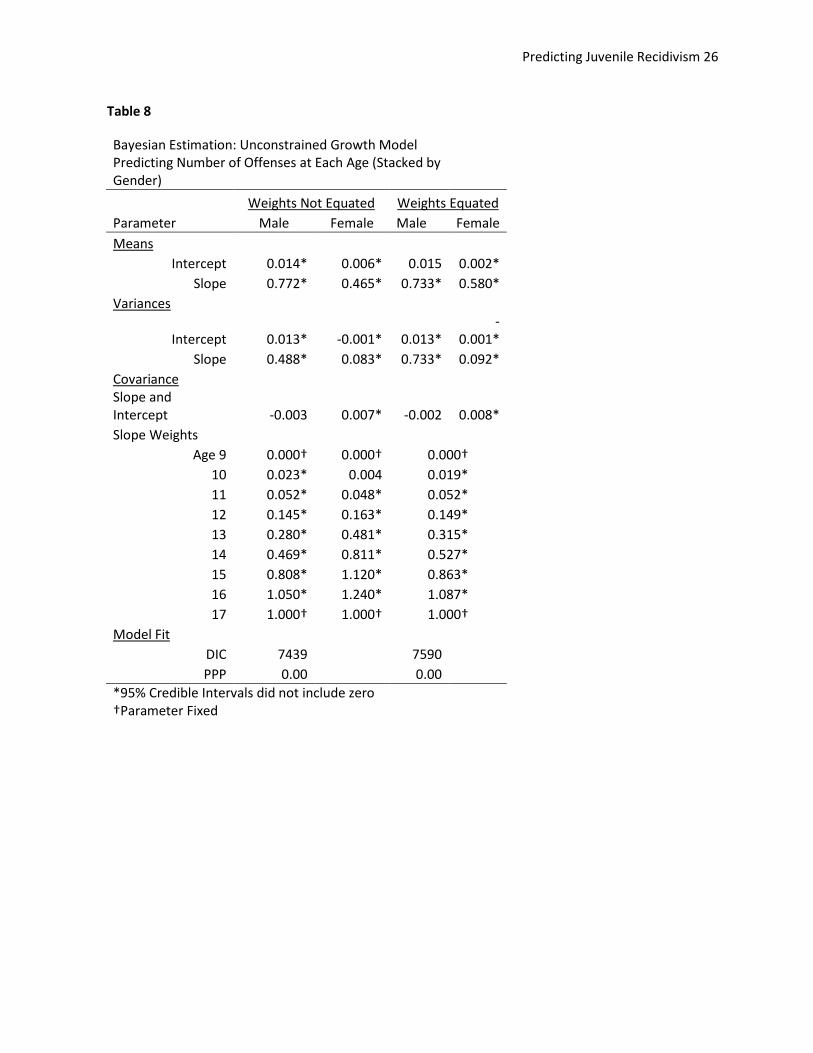
The deviance information criteria for the “weights not equated” model was reduced by 151, indicating
that the regression weights from the slope to each time point were significantly different across the
groups. (And simply adding gender as a second level predictor would violate the assumption of
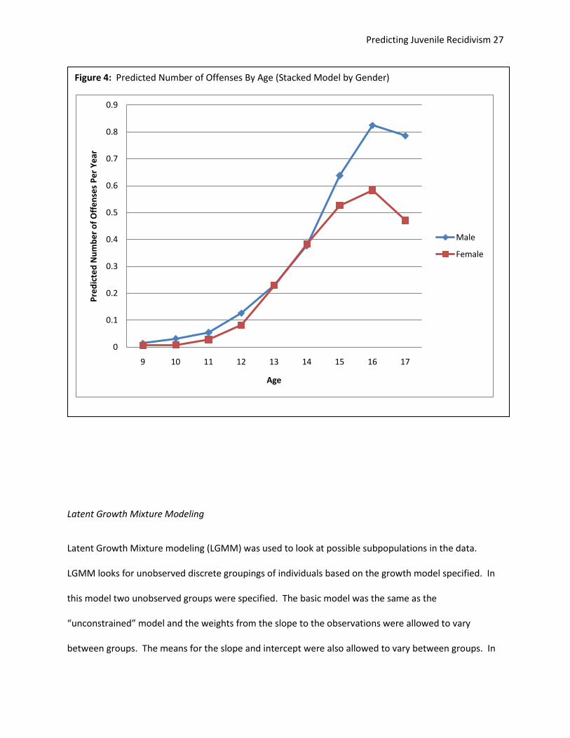
measurement invariance). As was expected, the female group had a lower mean slope, indicating that
females generally offend at a lower rate than males (in both the equated and non equated models, the
95% credible intervals for the two slopes did not overlap). Though females had lower average offending
rates, their trajectory peaked more sharply than their male counterparts (a maximum slope weight of
1.2 instead of 1.05). The prediction plot for the stacked model by gender with weights not equated can
be seen in figure 4.
Predicting Juvenile Recidivism 26
Table 8
Bayesian Estimation: Unconstrained Growth Model Predicting Number of Offenses at Each Age (Stacked by Gender)
Weights Not Equated Weights Equated
Parameter Male Female Male Female
Means Intercept 0.014* 0.006* 0.015 0.002*
Slope 0.772* 0.465* 0.733* 0.580*
Variances
Intercept 0.013* -0.001* 0.013* -
0.001*
Slope 0.488* 0.083* 0.733* 0.092*
Covariance Slope and
Intercept -0.003 0.007* -0.002 0.008*
Slope Weights Age 9 0.000† 0.000† 0.000†
10 0.023* 0.004 0.019*
11 0.052* 0.048* 0.052*
12 0.145* 0.163* 0.149*
13 0.280* 0.481* 0.315*
14 0.469* 0.811* 0.527*
15 0.808* 1.120* 0.863*
16 1.050* 1.240* 1.087*
17 1.000† 1.000† 1.000†
Model Fit DIC 7439
7590
PPP 0.00 0.00
*95% Credible Intervals did not include zero †Parameter Fixed
Predicting Juvenile Recidivism 27
Latent Growth Mixture Modeling
Latent Growth Mixture modeling (LGMM) was used to look at possible subpopulations in the data.
LGMM looks for unobserved discrete groupings of individuals based on the growth model specified. In
this model two unobserved groups were specified. The basic model was the same as the
“unconstrained” model and the weights from the slope to the observations were allowed to vary
between groups. The means for the slope and intercept were also allowed to vary between groups. In
Figure 4: Predicted Number of Offenses By Age (Stacked Model by Gender)
0
0.1
0.2
0.3
0.4
0.5
0.6
0.7
0.8
0.9
9 10 11 12 13 14 15 16 17
Pre
dic
ted
Nu
mb
er
of
Off
en
ses
Pe
r Y
ear
Age
Male
Female

Predicting Juvenile Recidivism 28
order to estimate this model, the variances were fixed for the slope and the intercept to 1. The errors
were also forced to be homoscedastic over time and equal across groups. Table 9 presents the Bayesian
estimates for the unconstrained LGMM with two groups.
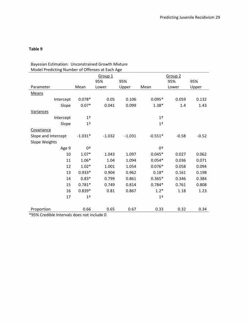
The estimated model picked out a first group that could best be described as very low level offenders
that stayed at a constant level of offending across time. Their predicted offending rate at age 9 was less
than one offense per 10 years and it increased by about that much over the course of adolescence. This
group (“group 1”) made up an estimated 66% of the total group.
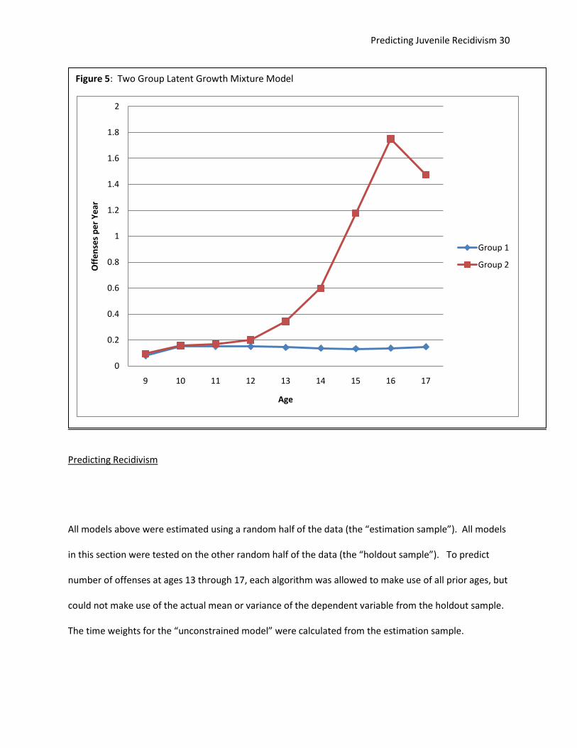
The second group made up 33% of the total sample and could best be described as moderate level
offenders who increased in offending and peaked at age 16 then returned to a lower rate at age 17.
Their predicted offending at age 9 was about the same as the first group, but they increased to an
average offending rate of 1.75 offenses per year. Their trajectories more closely resembled the original
group, but with a higher slope coefficient. Figure 5 shows the prediction plot for the latent growth
mixture model.
Predicting Juvenile Recidivism 29
Table 9
Bayesian Estimation: Unconstrained Growth Mixture Model Predicting Number of Offenses at Each Age
Group 1 Group 2
Parameter Mean 95% Lower
95% Upper Mean
95% Lower
95% Upper
Means Intercept 0.078* 0.05 0.106 0.095* 0.059 0.132
Slope 0.07* 0.041 0.099 1.38* 1.4 1.43
Variances Intercept 1†
1†
Slope 1†
1† Covariance
Slope and Intercept -1.031* -1.032 -1.031 -0.551* -0.58 -0.52
Slope Weights Age 9 0†
0†
10 1.07* 1.043 1.097 0.045* 0.027 0.062
11 1.06* 1.04 1.094 0.054* 0.036 0.071
12 1.02* 1.001 1.054 0.076* 0.058 0.094
13 0.933* 0.904 0.962 0.18* 0.161 0.198
14 0.83* 0.799 0.861 0.365* 0.346 0.384
15 0.781* 0.749 0.814 0.784* 0.761 0.808
16 0.839* 0.81 0.867 1.2* 1.18 1.23
17 1†
1†
Proportion 0.66 0.65 0.67 0.33 0.32 0.34
*95% Credible Intervals does not include 0
†Parameters fixed
Predicting Juvenile Recidivism 30
Predicting Recidivism
All models above were estimated using a random half of the data (the “estimation sample”). All models
in this section were tested on the other random half of the data (the “holdout sample”). To predict
number of offenses at ages 13 through 17, each algorithm was allowed to make use of all prior ages, but
could not make use of the actual mean or variance of the dependent variable from the holdout sample.
The time weights for the “unconstrained model” were calculated from the estimation sample.
Figure 5: Two Group Latent Growth Mixture Model
0
0.2
0.4
0.6
0.8
1
1.2
1.4
1.6
1.8
2
9 10 11 12 13 14 15 16 17
Off
en
ses
pe
r Y
ear
Age
Group 1
Group 2

Predicting Juvenile Recidivism 31
The “baseline model” was a guess of the average offenses per year at each age from the estimation
sample. This is a very sample dependent way of predicting recidivism, and does not discriminate
individuals, but does give some comparison for comparing mean absolute error values between models.
First, a “naïve” model was estimated. This is the model that would be used if a researcher did not
separate offenses by age, but simply added the priors together, and controlled for age as a linear
covariate. To estimate this model, a simple OLS linear regression was used at each age after 12. Prior
offenses in this model were just the sum of all previous offending events.
The unstandardized regression weights from the estimation sample were -.9235 for the intercept, .1379
for prior offenses and .0768 for current age.
For the “mean” model, each successive age point was modeled as the average of all previous time
points:
The “unconstrained” model estimated a slope and an intercept for each person (i), based on each prior
time point [t], in order to predict the future time points. The slope had an optimal weighting (that was
estimated in the previous section) at each time point .
Note: the are fixed in this model. The person parameters are all that are being estimated. This
problem is solved using a simple OLS matrix solution:

Predicting Juvenile Recidivism 32
Where the beta matrix is
, the X matrix is a column of ones and a column of the A[t]
weights. Y is a vector of the Y*t+’s. This is really estimating the best slope an intercept from a non-
linear trajectory that is already known.
Note that the Y[t] that this model is predicting is not in this OLS equation, only the prior time points are
used for estimation of the intercept and the slope. This design simulates actually predicting future time
points that have yet to occur.
Mean absolute error (MAE) was used as the measure of precision of the predicted number of offenses.
MAE is simply the average absolute value of the difference between the predicted Y and the observed Y.
This method gives less weights to outliers than methods that use sums of squares.
The latent growth mixture model (LGMM) utilized the two separate models estimated in the prior
section for unobserved groupings of the data. To determine which model to use, the two OLS slope and
intercepts based on the two sets of weights (A*t+’s) were both estimated. Then, maximum likelihood
was used to determine which sample the individual most likely came from. (Based on the mean slope
and intercepts estimated in the LGMM model). The likelihood function was:
Predicting Juvenile Recidivism 33
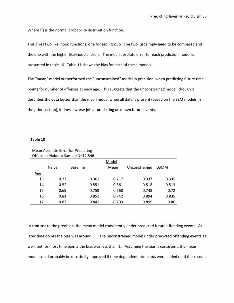
Where f() is the normal probability distribution function.
This gives two likelihood functions, one for each group. The two just simply need to be compared and
the one with the higher likelihood chosen. The mean absolute error for each prediction model is
presented in table 10. Table 11 shows the bias for each of these models.
The “mean” model outperformed the “unconstrained” model in precision, when predicting future time
points for number of offenses at each age. This suggests that the unconstrained model, though it
describes the data better than the mean model when all data is present (based on the SEM models in
the prior section), it does a worse job at predicting unknown future events.
In contrast to the precision, the mean model consistently under predicted future offending events. At
later time points the bias was around .5. The unconstrained model under predicted offending events as
well, but for most time points the bias was less than .1. Assuming the bias is consistent, the mean
model could probably be drastically improved if time dependent intercepts were added (and these could
Table 10
Mean Absolute Error for Predicting Offenses: Holdout Sample N=12,546
Model
Naïve Baseline Mean Unconstrained LGMM
Age 13 0.37 0.361 0.217 0.337 0.335
14 0.52 0.551 0.361 0.518 0.513
15 0.69 0.759 0.568 0.748 0.72
16 0.81 0.851 0.742 0.894 0.835
17 0.87 0.841 0.793 0.899 0.86

Predicting Juvenile Recidivism 34
be estimated by simply freeing up the intercepts on the SEM model, though one would still need to be
fixed for identification purposes).
Post-Hoc Analyses
Though not originally hypothesized, due to the poor model fit and poor predictive utility of the latent
growth model, an empirically determined residualized change model was examined. In this model, all
time points were predicted by each previous time point. The model for each time point was allowed to
have an intercept. This model was just identified in both the mean structure and the parameter
estimates.
Table 11
Bias for Predicting Offenses: Holdout Sample N=12,546
Model
Naïve Baseline Mean Unconstrained LGMM
Age 13 0.031 0.001 -0.165 -0.009 0.0001
14 0.001 -0.005 -0.268 -0.010 -0.009
15 -0.079 -0.003 -0.445 -0.012 -0.004
16 -0.091 -0.002 -0.564 -0.060 0.001
17 0.071 -0.01 -0.515 -0.130 -0.007

Predicting Juvenile Recidivism 35
Because it was just identified, there was no model fit for this structural equation model. But an
examination of the parameter estimates revealed that almost every time point was significantly
predicted by just the previous two time points and the intercept. This suggests for future studies, that
though much less elegant, a residualized change model where each time point is predicted by the
previous two time points and an intercept may adequately describe the data. It is more than likely that
the B parameters capitalize on chance to a large degree and may not be estimated consistently from
dataset to dataset. (Which would make them poor candidates for prediction models).
Cross Validation of Unconstrained Model
Predicting Juvenile Recidivism 36
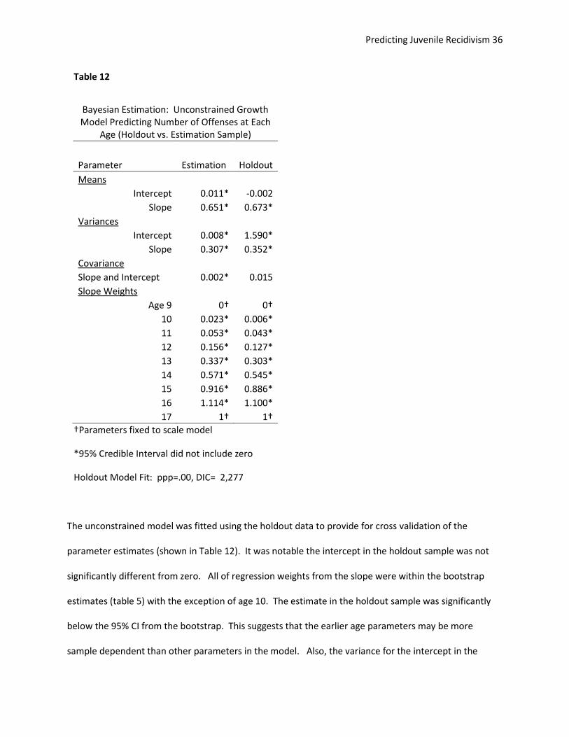
The unconstrained model was fitted using the holdout data to provide for cross validation of the
parameter estimates (shown in Table 12). It was notable the intercept in the holdout sample was not
significantly different from zero. All of regression weights from the slope were within the bootstrap
estimates (table 5) with the exception of age 10. The estimate in the holdout sample was significantly
below the 95% CI from the bootstrap. This suggests that the earlier age parameters may be more
sample dependent than other parameters in the model. Also, the variance for the intercept in the
Table 12
Bayesian Estimation: Unconstrained Growth Model Predicting Number of Offenses at Each
Age (Holdout vs. Estimation Sample)
Parameter Estimation Holdout
Means Intercept 0.011* -0.002
Slope 0.651* 0.673*
Variances Intercept 0.008* 1.590*
Slope 0.307* 0.352*
Covariance Slope and Intercept 0.002* 0.015
Slope Weights Age 9 0† 0†
10 0.023* 0.006*
11 0.053* 0.043*
12 0.156* 0.127*
13 0.337* 0.303*
14 0.571* 0.545*
15 0.916* 0.886*
16 1.114* 1.100*
17 1† 1†
†Parameters fixed to scale model
*95% Credible Interval did not include zero
Holdout Model Fit: ppp=.00, DIC= 2,277

Predicting Juvenile Recidivism 37
holdout sample was several times larger than the one estimated in the previous sample. The parameter
on age 16 was not only different from zero, but it was also different from 1, suggesting that the peak at
age 16 with a decrease to age 17 is not a sample dependent phenomenon.
The predictive utility of this unconstrained model was similar to the original estimation sample (see
table 13). The MAE values were greater than the ones predicted by the mean, but the bias was similarly
small. This also would not function as a good predictive model for offending.
Table 13
Predicting the Estimation Sample Using the Estimated Weights From the Holdout
Sample
MAE Bias
Age 13 0.36 0.007
14 0.54 0.017
15 0.76 -0.009
16 0.91 -0.053
17 0.92 -0.11

Predicting Juvenile Recidivism 38
Discussion
From these results, it would appear that a latent growth curve model is not necessarily the best way to
predict future offending behavior. But what we can learn from this model is that there is good support
for the idea that the age-crime curve is not just a group phenomenon, but an individual phenomenon.
In other words, Moffit originally thought that the age crime curve was something that occurred because
more individuals began offending during the middle of adolescence, but that during an individual’s
active offending period, that offending is relatively constant. What the “unconstrained” model tell us is
that for an individual offending generally increases and then decreases through adolescence. In other
words, there is something like an age-crime curve for each person.
The latent growth mixture modeling adds a more nuanced version of this individual age crime curve.
This model shows us that 66% of the general population has a roughly equal chance of offending during
the course of their adolescence. And they are probably only going to offend once and then never again.
These youth, apart from adolescent limited youth, are “one timers,” but they have roughly the same
probability of offending at any age. This is in contrast to the idea of adolescent limited youth, who
offend just during middle-late adolescence.
The second group, make up about a third of the general offender population. These are the individuals
who offend multiple times and increase up to age 16 and then decrease. These are the offending youth
who really influenced the general model to show an individual age crime curve. Based on the mixture
modeling, it appears that these frequent offending youth really make up a smaller proportion of the
overall population, but because they offend so much more than the “one timers” (they peak at almost
two offenses per year) they heavily influence the general model.

Predicting Juvenile Recidivism 39
Surprisingly, this study found that the “naïve” model, or the model that ignores the age of each offense,
is not drastically worse than models that take into account the age of each offense. This finding could
be due to the fact that this sample contains so many of the “one time” offenders identified by the
mixture model. Nonetheless, there is no evidence that using models that just control for age as a linear
covariate will result in findings that are drastically biased, but these models will not improve prediction
much beyond guessing the mean either.
It should be noted that structural equation model fit does not necessarily measure what model will best
predict future offending events. This is because model fit is measuring how well the model reproduces
all of the relationships in a given data set. For predicting offending events, certain relationships cannot
plausibly be used (for example, the causal path from age 17 to age 9).
Overall, models that just look at number of offenses at each age may be too simplistic to capture what is
really causing offending that persists, versus offending that desists. Models that take more variables
into account are likely needed to better predict future offending events. Future directions for research
might include looking at the stability across samples of residualized change scores. Also, more
sophisticated models that take into account types of offenses at each age may still leave a more
promising avenue for latent growth modeling of offending events.

Predicting Juvenile Recidivism 40
Works Cited
Duncan, T. & Duncan, S. (2004). An introduction to latent growth curve modeling. Behavior Therapy.
35, 333-363.
Farrington, D.P. (2005). Introduction to integrated developmental and life-course theories of offending.
D.P. Farrington (ed.) Integrated Developmental and Life-Course Theories of Offending (pp. 1-13). New
Brunswick, NJ: Transaction Publishers
Lee, S. (2007). Structural Equation Modeling: A Bayesian Approach. West Sussex, England: Wiley.
Loeber, R. & Farrington, D. (2000). Young children who commit crime: epidemiology, developmental
origins, risk factors, early interventions and policy implications. Developmental Psychopathology. 12,
737-762.
Loeber, R. & Snyder, H.N. (1990). Rate of offending in juvenile careers: findings of constancy and change
in lambda. Criminology. 28 (1), 97-109.
Mason, A.W. (2001). Self-Esteem and delinquency revisited (again): a test of Kaplan’s self-derogation
theory of delinquency using latent growth curve modeling. Journal of Youth and Adolescence. 30 (1),
84-102.
McArdle, J.J., & Nesselroade, J.R. (2003). Growth curve analysis in contemporary psychological research.
In J.A. Schinka,& W.F. Velicer (Ed.) Research Methods in Psychology (pp. 447-482). Hoboken, NJ: John
Wiley and Sons.
Moffit, T. (1993). Adolescent limited and life-course-persistent antisocial behavior: a developmental
taxonomy. Psychological Review. 100 (4), 674-701.

Predicting Juvenile Recidivism 41
Scheines, R., Hoijtink, H. & Boomsma, A. (1999). Basyesian estimation and testing of structural equation
models. Psychometrika. 64 (1), 37-52.
Stolzenberg, L. & D’Alessio, S.J. (2008). Co-offending and the age crime curve. Journal of Research in
Crime and Delinquency, 45, 65-86.
Stoolmiller, M. (1994) Antisocial behavior, delinquent peer association and unsupervised wandering for
boys: growth and change from childhood to early adolescence. Multivariate Behavioral Research, 29
(3), 263-288.
Wiesner, M. & Windle, M. (2004). Assessing covariates of adolescent delinquency trajectories. Journal
of Youth and Adolescence. 33 (5), 431-442.