IT 13 055

Examensarbete 15 hpAugusti 2013

Intelligent Online Marketing

Predicting Conversion Rate Of New Keywords

Tommy Engström

Institutionen för informationsteknologiDepartment of Information Technology

.

Teknisk- naturvetenskaplig fakultet UTH-enheten Besöksadress: Ångströmlaboratoriet Lägerhyddsvägen 1 Hus 4, Plan 0 Postadress: Box 536 751 21 Uppsala Telefon: 018 – 471 30 03 Telefax: 018 – 471 30 00 Hemsida: http://www.teknat.uu.se/student

Abstract

Intelligent Online Marketing

Tommy Engström

This thesis looks at the problem of predicting conversion rate ofkeywords in Google Adwords where little or no data for the keyword is available.Several methods are investigated and tested on data belonging to threedifferent real world clients. The methods try to predict the conversion rate only giventhe keyword text. All methods are compared, using two different evaluation methods,with results showing good potential. Finally further improvements are suggested thatcould have a big impact on the results.

Tryckt av: Reprocentralen ITCIT 13 055Examinator: Olle GällmoÄmnesgranskare: Michael AshcroftHandledare: Anders Arpteg

.

Contents

1 Introduction 41.1 Abbreviations And Definitions . . . . . . . . . . . . . . . . . . . 41.2 Background . . . . . . . . . . . . . . . . . . . . . . . . . . . . . . 41.3 Problem Description . . . . . . . . . . . . . . . . . . . . . . . . . 5

2 Methods 62.1 Introduction to the used tools . . . . . . . . . . . . . . . . . . . . 6

2.1.1 Python . . . . . . . . . . . . . . . . . . . . . . . . . . . . 62.1.2 NumPy . . . . . . . . . . . . . . . . . . . . . . . . . . . . 62.1.3 Pandas . . . . . . . . . . . . . . . . . . . . . . . . . . . . 62.1.4 Matplotlib . . . . . . . . . . . . . . . . . . . . . . . . . . . 72.1.5 Scikit-learn . . . . . . . . . . . . . . . . . . . . . . . . . . 72.1.6 Orange . . . . . . . . . . . . . . . . . . . . . . . . . . . . 7

2.2 Preprocessing . . . . . . . . . . . . . . . . . . . . . . . . . . . . . 72.2.1 Data Formats . . . . . . . . . . . . . . . . . . . . . . . . . 7

2.3 Inferring CR from other statistics . . . . . . . . . . . . . . . . . . 82.3.1 Motivation . . . . . . . . . . . . . . . . . . . . . . . . . . 82.3.2 Data Exploration . . . . . . . . . . . . . . . . . . . . . . . 82.3.3 Algorithm Used . . . . . . . . . . . . . . . . . . . . . . . . 9

2.4 Term Model . . . . . . . . . . . . . . . . . . . . . . . . . . . . . . 122.4.1 Motivation . . . . . . . . . . . . . . . . . . . . . . . . . . 122.4.2 Preprocessing . . . . . . . . . . . . . . . . . . . . . . . . . 122.4.3 Data Exploration . . . . . . . . . . . . . . . . . . . . . . . 132.4.4 Weighted Linear Combination Model . . . . . . . . . . . . 152.4.5 Binary Word Model . . . . . . . . . . . . . . . . . . . . . 152.4.6 K-Nearest Neighbor . . . . . . . . . . . . . . . . . . . . . 162.4.7 Distance Weighted K-Nearest Neighbor . . . . . . . . . . 182.4.8 Random Forest . . . . . . . . . . . . . . . . . . . . . . . . 18

3 Results 193.1 The Problem In Evaluating Results . . . . . . . . . . . . . . . . . 193.2 Evaluation Method 1 . . . . . . . . . . . . . . . . . . . . . . . . . 19

3.2.1 Result Presentation Method . . . . . . . . . . . . . . . . . 203.2.2 Mean Prediction Results . . . . . . . . . . . . . . . . . . . 20

1

3.2.3 CTR Regression Results . . . . . . . . . . . . . . . . . . . 203.2.4 Term Model Results . . . . . . . . . . . . . . . . . . . . . 21

3.3 Evaluation Method 2 . . . . . . . . . . . . . . . . . . . . . . . . . 303.3.1 Mean Prediction Results . . . . . . . . . . . . . . . . . . . 30

3.4 Result Analysis . . . . . . . . . . . . . . . . . . . . . . . . . . . . 38

4 Future Improvements 40

5 Critical Analysis 41

2

Chapter 1

Introduction

1.1 Abbreviations And Definitions

BR Bounce Rate, V isits−NonV isitsV isits

Broad match Matching any search query that Google consider similarClicks The number of times someone clicked on the adConversions The number of times the ad led to a purchase or

some other desirable actionCR Conversions Rate, Conversions

Clicks

CTR Click Through Rate, ClicksImpressions

Exact match Matching only the exact phraseImpressions The number of times an ad have been shownLong tail keyword Keyword with very low trafficNonVisit When a user visits a site but performed no further actionMatch type How keywords match with a search phrasePhrase match Matching search queries containing the phraseRMSE Root Mean Squared ErrorVisit When a user visits a siteVPC Value Per Click

1.2 Background

The work was done at Campanja in their office on Kungsgatan 27, Stockholm.Campanja provides a bidding platform for online advertising that strives todeliver high performance through intelligent real time analysis of data.

One of the most important tasks that Campanja’s software performs is tosubmit bids in online ad auctions. For search campaigns, search queries arematched to advertisers requests for advertising, in the form of bids for keywords.E.g. a user searches for white widgets (this is called the search query). There

3

are three advertisers willing to be shown for the word widgets (called a keyword,with an associated match type), and two willing to be shown for white widgets.They will all be ordered by their respective bids and shown on the search page.When a user clicks an ad, the advertiser is charged the price the advertiser withthe second highest bid was willing to pay. In reality this process is more complexand also uses quality score, which is how relevant Google think the ad is, andother factors. The true formula is subject to change and not public.

These auctions take place millions of time per day. Auctions are run on a persearch basis and affected by bid, relevancy and many more factors. However,from an advertisers point of view, an auction and the subsequent click is justthe beginning of a process, that, ideally, leads to the user purchasing somethingor making another desirable action on the advertisers website. Such a desirableaction is usually called a conversion, i.e. the user converts from being just avisitor to becoming a customer. The fraction of users that make a conversion iscalled the conversion rate, CR. The CR must be big enough for the advertiserto make a profit. It is thus essential to try to figure out the conversion rate inadvance, to be able to set a correct bid.

1.3 Problem Description

Ads on Google Adwords are paid for by click, if there is no click there is nocost. The key metric when determining how much one should be willing to payfor an ad is the Value Per Click, VPC, which is defined as V PC = ConversionRate× Conversion V alue.

The objective of this thesis is to predict the Conversion Rate, CR, for key-words with little or no data. This is very important since a single customer canhave several million active keywords. Many keywords have far to little data tocalculate any significant statistics, but combined they make up for a big chunkof the total conversions.

4

Chapter 2

Methods

All code was written in Python using appropriate libraries. It was a clear choicesince it is very suitable for the task and what is currently used for such tasks atCampanja.

2.1 Introduction to the used tools

2.1.1 Python

Python [1] is a dynamically typed, interpreted high level language aiming forhigh readability and productivity. There are several good machine learninglibraries and data analysis available for it.

2.1.2 NumPy

NumPy [2], short for Numerical Python, is a math library for Python. Thecentral part of NumPy is the array for which there are very well optimized Cand Fortran functions for linear algebra and manipulation. Many libraries arebuild upon NumPy.

2.1.3 Pandas

Pandas [3] is a library providing high performance data structures for Pythonbased on NumPy arrays. It provides R-style data frames and very powerfulmethods for data manipulation. Table 2.1 show a short example of how Pandasis used.

5

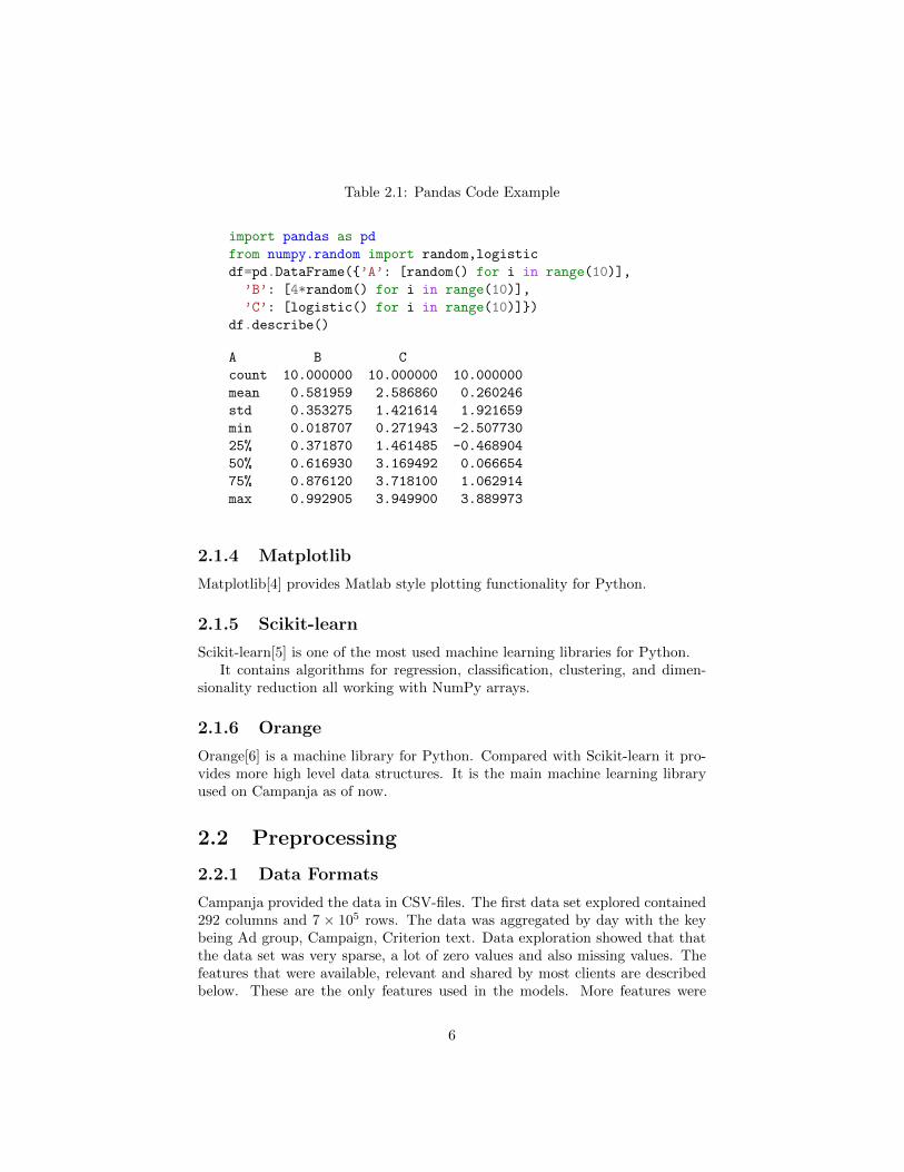
Table 2.1: Pandas Code Example

import pandas as pd

from numpy.random import random,logistic

df=pd.DataFrame({’A’: [random() for i in range(10)],

’B’: [4*random() for i in range(10)],

’C’: [logistic() for i in range(10)]})

df.describe()

A B C

count 10.000000 10.000000 10.000000

mean 0.581959 2.586860 0.260246

std 0.353275 1.421614 1.921659

min 0.018707 0.271943 -2.507730

25% 0.371870 1.461485 -0.468904

50% 0.616930 3.169492 0.066654

75% 0.876120 3.718100 1.062914

max 0.992905 3.949900 3.889973

2.1.4 Matplotlib

Matplotlib[4] provides Matlab style plotting functionality for Python.

2.1.5 Scikit-learn

Scikit-learn[5] is one of the most used machine learning libraries for Python.It contains algorithms for regression, classification, clustering, and dimen-

sionality reduction all working with NumPy arrays.

2.1.6 Orange

Orange[6] is a machine library for Python. Compared with Scikit-learn it pro-vides more high level data structures. It is the main machine learning libraryused on Campanja as of now.

2.2 Preprocessing

2.2.1 Data Formats

Campanja provided the data in CSV-files. The first data set explored contained292 columns and 7 × 105 rows. The data was aggregated by day with the keybeing Ad group, Campaign, Criterion text. Data exploration showed that thatthe data set was very sparse, a lot of zero values and also missing values. Thefeatures that were available, relevant and shared by most clients are describedbelow. These are the only features used in the models. More features were

6

available but was omitted because of unreliable values, which became obviousafter plotting the data.

• Clicks

• Conversions

• Impressions

• Ad group Name

• Campaign Name

• Criterion Text

2.3 Inferring CR from other statistics

2.3.1 Motivation

A problem with CR is that a fair amount of data is needed to get a goodestimation of the true CR. Conversions are much more scarce than clicks, oftenmore than 50 times so. The initial idea is to predict CR using statistics forwhich we gather data more rapidly. Two statistics that could be potentially beused is Click Through Rate, CTR, and Bounce Rate, BR.

2.3.2 Data Exploration

To see whether or not a model based on this would be likely to help in predictingCR I started off by examining to see how it’s distributed and to find correlations.

Conversion Rate Distributions

Figure 2.1 shows the distribution of CR for different keywords on different clientsfor keywords with at least 100 clicks. The figures indicate that different clientscan have very different properties and could potentially need to be treated dif-ferently.

CR-CTR Correlation

Figure 2.2 shows scatter plots of CR and CTR and Table 2.2 shows the PearsonCorrelation Coefficients, PCC. PCC is the co-variance divided by the product

of the standard deviations, defined as ρX,Y = cov(X,Y )σXσY

[7]. It results in a valuebetween −1 and 1 with 0 representing no correlation and the sign representingthe direction of the correlation, e.g a PCC value of 1 would imply that if theCTR were to double so would the CR. PCC assumes both CR and CTR arenormally distributed, which is not exactly true but a reasonable approximation.

All keywords with less than 100 clicks were filtered out. The plot for Client3 looks very suspect. It turned out that the data had been tempered with inorder to make up for the problems of having very sparse data.

7

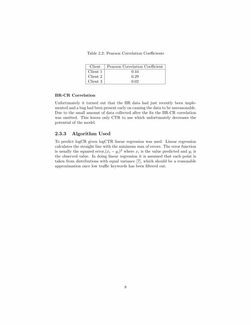
Table 2.2: Pearson Correlation Coefficients

Client Pearson Correlation CoefficientClient 1 0.44Client 2 0.29Client 3 0.02

BR-CR Correlation

Unfortunately it turned out that the BR data had just recently been imple-mented and a bug had been present early on causing the data to be unreasonable.Due to the small amount of data collected after the fix the BR-CR correlationwas omitted. This leaves only CTR to use which unfortunately decreases thepotential of the model.

2.3.3 Algorithm Used

To predict logCR given logCTR linear regression was used. Linear regressioncalculates the straight line with the minimum sum of errors. The error functionis usually the squared error,(xi − yi)2 where xi is the value predicted and yi isthe observed value. In doing linear regression it is assumed that each point istaken from distributions with equal variance [7], which should be a reasonableapproximation once low traffic keywords has been filtered out.

8

Figure 2.1: CR Distributions

9

Figure 2.2: CR-CTR Correlation

10

2.4 Term Model

2.4.1 Motivation

The goal of this model is to be able use the information about words present in akeyword in a more elaborate way. The idea is to construct a model that exploitsthe information of what particular words are present and uses it to predict theconversion rate. Another good thing about this is that the statistics for wordsreach significant levels quicker than statistics for keywords. This allows for away to estimate the value of a keyword when we have statistics for the words,or at least some of them, but none at all for the keyword.

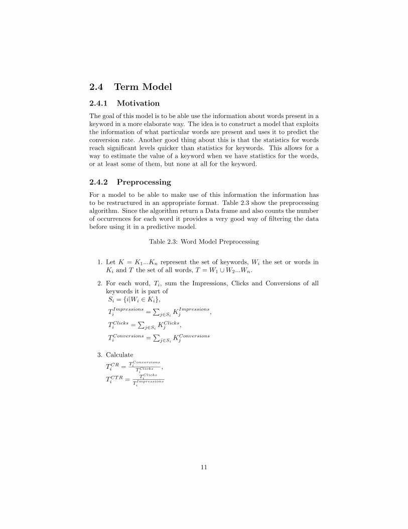
2.4.2 Preprocessing

For a model to be able to make use of this information the information hasto be restructured in an appropriate format. Table 2.3 show the preprocessingalgorithm. Since the algorithm return a Data frame and also counts the numberof occurrences for each word it provides a very good way of filtering the databefore using it in a predictive model.

Table 2.3: Word Model Preprocessing

1. Let K = K1...Kn represent the set of keywords, Wi the set or words inKi and T the set of all words, T = W1 ∪W2...Wn.

2. For each word, Ti, sum the Impressions, Clicks and Conversions of allkeywords it is part ofSi = {i|Wi ∈ Ki},

T Impressionsi =∑j∈Si

KImpressionsj ,

TClicksi =∑j∈Si

KClicksj ,

TConversionsi =∑j∈Si

KConversionsj

3. Calculate

TCRi =TConversionsi

TClicksi

,

TCTRi =TClicksi

T Impressionsi

11

Table 2.4: Keyword data to word data

Keyword Text Impressions Clicks Conversions CR CTRmovies online 1200 225 20 0.09 0.19free movies 1500 154 3 0.02 0.10action movies 210 107 17 0.16 0.51

Word Impressions Clicks Conversions CR CTRaction 210 107 17 0.16 0.51free 1500 154 3 0.02 0.10

movies 2910 486 40 0.08 0.17online 1200 225 20 0.09 0.19

2.4.3 Data Exploration

Figure 2.3 show the distribution of CR on word level for two customers the redline marks the average CR. The figures show that the CR per word is aboutas spread as the CR per keyword, making it seem very plausible that there isinformation to be extracted this representation.

12

Figure 2.3: Distributions of word CR

13

2.4.4 Weighted Linear Combination Model

Motivation

The idea behind this method is to use the CR of the individual words of thekeyword to predict the CR of the keyword. By calculating statistics for individ-ual words we get statistics with high confidence sooner which allows the modelto take advantage of data for the client even when there is no data availablefor the given keyword. Although it seems very likely this information could beused to make an estimate of the CR it is not obvious how to combine the wordestimates in a good way. The following sections describes the approaches tested.

Algorithms

To find a good way to combine the statistics of individual words into a predictionof the CR for a keyword several different formulas were tried. Table 2.5 showsthe formulas initially tested.

The formulas in Table 2.5 represent different ways to combine the words yetthey fail to take into account the importance of individual words. With that inmind a weighted average formula as shown in table 2.6 was proposed. It’s builtupon the idea that words with CR that deviate more from the average CR willbe more important. In the case where statistic was not available for a word theaverage CR was used, giving that word zero weight.

Table 2.5: CR Combining Formulas

Average CR K = 1n

∑Wn

i=W1Wi

Max CR K = Max(Wi)Min CR K = Min(Wi)

K=Keyword CR, W=Word CR, A=Average CR, n = Number of words in Keyword

Table 2.6: Weighted Average Formula

1. Calculate the weight constants, C ′Wi= Wi −Kmean, i = 0...n

2. Normalize, CWi=

C′Wi∑C′

W

3. Calculate the new CR as, K =∑ni=0 CWi

Wi

2.4.5 Binary Word Model

To be able to use common machine learning algorithms predicting the CR thedata had to be restructured in a suitable format. The format proposed is basedon binary features representing the occurrence of a word along with natural

14

number for features representing the number of words and the number of un-known words. Unknown words show up when words are filtered out or whencompletely new words show up in the test set. Table 2.7 shows the algorithmand 2.8 shows the format of the data for a made-up data set.

Table 2.7: Binary word model creation algorithm

1. Calculate word statistics as described in 2.3.

2. Mij =

{1 ,Wi ∈ Ki

0 ,Wi /∈ Ki, where K and W are the sets of keywords and

words.

3. Save Mij together with Ki and CRi

Table 2.8: Example of training data

Wcount Ucount buy food pizza sushi CR2 0 1 1 0 0 0.043 1 1 1 0 0 0.022 0 1 0 0 1 0.093 1 0 0 1 1 0.054 2 1 0 1 0 0.11

Wcount represent word count and Ucount represent the count of unknown words.

2.4.6 K-Nearest Neighbor

KNN is very suitable for this data format. The data is structured in such a waythat keywords that share words and length will be considered similar. It is alsoa good base approximation to compare other methods to [8]. The algorithmworks as described in Table 2.9.

Table 2.9: KNN Regression Algorithm

1. Define the distance as between a keyword, W , and the target, T , as∑Ni=1 |Wi − Ti|,where i is the column as shown in table 2.8 and N is the

number of word.

2. Let N be the set of CRs for the K keywords closest by distance to thetarget keyword.

3. Calculate estimated target CR as 1K

∑Ki=1Ni

15

Table 2.10: KNN Example

The CR prediction of “buy pizza or kebab” given the data in Table 2.9 andK = 2.

1. Convert to the format of Table 2.9 and call it P :

Wcount Ucount buy food pizza sushi3 1 1 0 1 0

The word “or” was not part of the set of words and are thus counted asan unknown word.

2. Calculate the distance to each sample in table 2.9 as Distancei =∑j∈features (Sij − Pj)2, where S are the samples from the training data.

Wcount Ucount buy food pizza sushi Distance(2− 3)2 (0− 1)2 (1− 1)2 (1− 0)2 (0− 1)2 (0− 0)2 4(3− 3)2 (1− 1)2 (1− 1)2 (1− 0)2 (0− 1)2 (0− 0)2 2(2− 3)2 (0− 1)2 (1− 1)2 (0− 0)2 (0− 1)2 (1− 0)2 4(3− 3)2 (0− 1)2 (0− 1)2 (0− 0)2 (1− 1)2 (1− 0)2 3(4− 3)2 (2− 1)2 (1− 1)2 (0− 0)2 (1− 1)2 (0− 0)2 2

3. Average the value of the 2 samples with the shortest distance to the target,(−2.56+(−4.12))

2 = −3.34

16

2.4.7 Distance Weighted K-Nearest Neighbor

This approach comes from the intuition with a CR that diverges a lot from theaverage will likely influence the keyword’s CR more. Research have shown thatusing distance weighting can allow the algorithm to use a higher K, which makesit more robust [9]. The algorithm used is the same but instead of using binaryfeatures for each word they are represented with a scalar, di = |Wi − A|, thatrepresent the words distances from the average CR.

Given that the average CR is 6% and the word “pizza” has a CR of 14% athe weight of the “pizza” feature would be |0.14− 0.06| = 0.08. If the keywordalso contains the word “salad” with a CR of 7% that word will influence thedistance to other keywords less.

2.4.8 Random Forest

Random forest is an ensemble method consisting of a number of decision trees.A regression decision tree is a binary tree with each node containing a splittingcriterion and each leaf containing a scalar. Figure 2.4 show a minimal randomforest with two trees. If used to calculate thee CR of “free action movie” itwould predict 0.01+0.02

2 = 0.015The downside with decision trees is that the tend to over fit the data unless

there ability to split is restricted. In a random forest the high variance problemis countered by using an ensemble of decision trees trained on different subsetsof the data. Since each tree is trained on a different sample they will all havedifferent sample errors. It can be shown that given a sufficient number of treesa random forest will always converge [10].

Random forests are also robust, the algorithm will never predict a valueoutside the range of values seen in the training data which make it less sensitiveto outliers is the test data. Another benefit is that very little tweaking ofparameters is needed since the over fitting problem is handled by the ensemblegiven that enough trees are used.

Figure 2.4: Random forest example

Includes “free”

0.01Includes

“Comedy”

0.020.04

yes no

yes no

Includes

“Movie”

0.02Includes “Free”

0.070.01

yes

no

yes no

17

Chapter 3

Results

3.1 The Problem In Evaluating Results

3.2 Evaluation Method 1

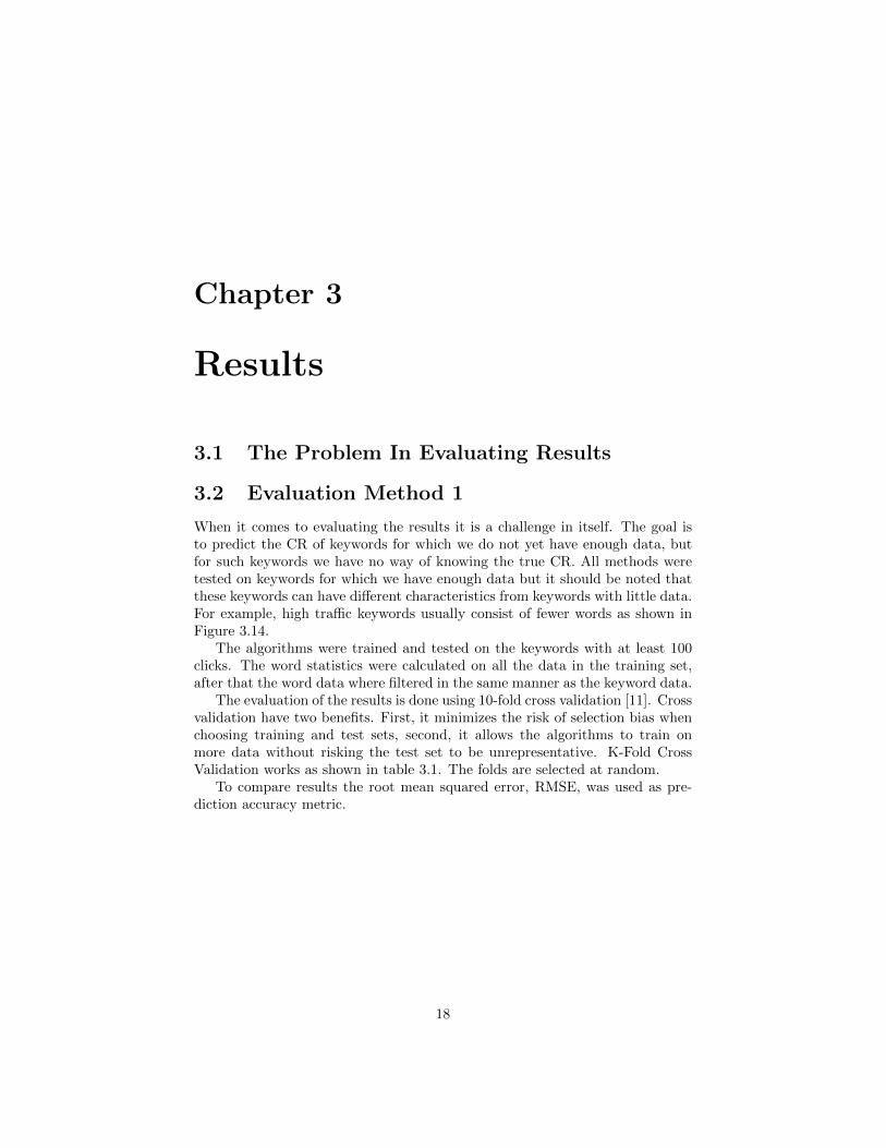
When it comes to evaluating the results it is a challenge in itself. The goal isto predict the CR of keywords for which we do not yet have enough data, butfor such keywords we have no way of knowing the true CR. All methods weretested on keywords for which we have enough data but it should be noted thatthese keywords can have different characteristics from keywords with little data.For example, high traffic keywords usually consist of fewer words as shown inFigure 3.14.

The algorithms were trained and tested on the keywords with at least 100clicks. The word statistics were calculated on all the data in the training set,after that the word data where filtered in the same manner as the keyword data.

The evaluation of the results is done using 10-fold cross validation [11]. Crossvalidation have two benefits. First, it minimizes the risk of selection bias whenchoosing training and test sets, second, it allows the algorithms to train onmore data without risking the test set to be unrepresentative. K-Fold CrossValidation works as shown in table 3.1. The folds are selected at random.

To compare results the root mean squared error, RMSE, was used as pre-diction accuracy metric.

18

Table 3.1: K-Fold Cross Validation

1. Split the data into K sets

2. Take away 1 set for testing

3. Train an algorithm on K − 1 of the sets

4. Test the algorithm on the test set

5. Iterate using every set as test set once

6. Use all test results as total result

3.2.1 Result Presentation Method

The result for each model is visualized using a scatter plot showing the pre-diction compared to the observed value. The plot also contain a line diagonalrepresenting perfect correlation. The RMSE is calculated for each plot and pre-sented in the title and a summary of all RMSE improvements versus mean ispresented in a table.

3.2.2 Mean Prediction Results

The plots in figure 3.1 show the prediction performance when assigning theaverage CR to every keyword. This is used as a benchmark for all other modelsand should also be a good estimate of what the current system would predicttoday.

Each plot contains 10 individual lines, one for each fold. For Client 2 and3 this is barely visible using this scale but for Client 1 there is a big gap. Itturns out that Client 1 has over 40% of it’s total ad-clicks coming from a singlekeyword. The keyword has a CR of 9.1% instead of the average 7.1%, whichactually brings the average CR of all other keywords to 5.6%.

3.2.3 CTR Regression Results

Figure 3.2 show the results of the CTR Regression model. The model signifi-cantly improves the predictions for client 1, which is to be expected since Client1 had the strongest correlation between CTR and CR.

The result for Client 3 is a great example of when linear regression goeswrong. The method has no good way of handling outliers.

19

3.2.4 Term Model Results

Weighted Average Formula Results

The weighted average formula turned out to be superior over other formulasproposed in 2.4.4. Figure 3.3 shows the results for the weighted average formula.

K-Nearest Neighbor

For all these plots K = 3 was used. This turned out to be a good fit for all datasets but it is dependent on the number of instances in the data set. The resultsare presented in figure 3.4.

Distance Weighted K-Nearest Neighbor

In the distance weighted KNN version a K = 5 was used. The distance weighingmade it so that the K-value could be increased without dropping performance.Figure 3.5 shows the results of the predictions.

Random Forest

The random forest uses 20 decision trees, increasing the number of trees hadlittle influence on the prediction results. The results are shown in Figure 3.6

Model Combinations

In addition to the models described in the previous chapter a number of combi-nations of models were tested. The best combination was using weighted average+ random forest. The model predicts the CR to be the unweighted average ofthe two models.

The result for the combination of models are shown in Figure 3.13.

Summary

Table 3.2 shows a shows the RMSE of every model divided by the RMSE ofthe mean-based model. This method was chosen to make it easy to compareperformance of the algorithms for different clients, since the RMSE varies a lotbetween them.

20

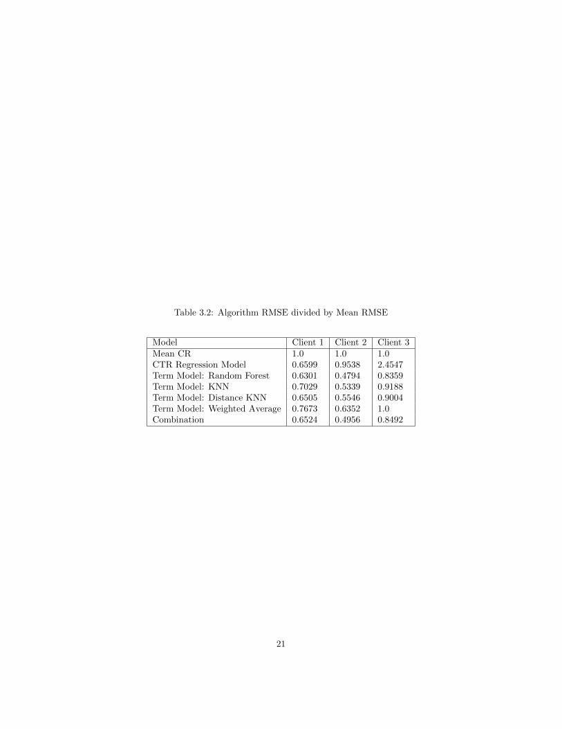
Table 3.2: Algorithm RMSE divided by Mean RMSE

Model Client 1 Client 2 Client 3Mean CR 1.0 1.0 1.0CTR Regression Model 0.6599 0.9538 2.4547Term Model: Random Forest 0.6301 0.4794 0.8359Term Model: KNN 0.7029 0.5339 0.9188Term Model: Distance KNN 0.6505 0.5546 0.9004Term Model: Weighted Average 0.7673 0.6352 1.0Combination 0.6524 0.4956 0.8492

21

Figure 3.1: Mean Prediction Results

22

Figure 3.2: CTR Regression Results

23

Figure 3.3: Formula Approach

24

Figure 3.4: KNN

25

Figure 3.5: Distance Weighted KNN

26

Figure 3.6: Random Forest

27

Figure 3.7: Combination: Weighted Average + Random Forest

28

3.3 Evaluation Method 2

To test the models on data from actual long tail keywords an aggregation methodwas constructed. The idea is to combine several keywords into one and use thepredictions for each individual keyword weighed together as the group result.The algorithm works as described below.

1. Predict the number of conversions for each keyword.

2. Group keywords together so that each group has at least 500 clicks com-bined.

3. Divide the combined number of conversions with the combined number ofclicks.

The algorithms were trained on all the keywords with at least 100 clicks.The word data was calculated from all keywords with 50 clicks or more and thetesting were done using keywords with less than 50 clicks.

3.3.1 Mean Prediction Results

The plots in figure 3.8 show the prediction performance when assigning theaverage CR to every keyword. This is used as the benchmark for the othermodels.

Weighted Average Results

Figure 3.9 show the result for the weighted average formula.

K-Nearest Neighbor

Figure 3.10 show the result of the KNN model on the long tail keywords. Justas when testing on keywords with more data K = 3 was used.

Distance Weighted K-Nearest Neighbor

Figure 3.11 show the results of the distance weighted KNN model using K = 5.

Random Forest

Figure 3.12 show the performance of the Random Forest predictor using 20trees.

Model Combinations

In addition to the models described in the previous chapter a number of combi-nations of models were tested. The best combination was using weighted average+ random forest. The model predicts the CR to be the unweighted average ofthe two models.

The result for the combination of models are shown in Figure 3.13.

29

Summary

Table 3.3 shows a shows the RMSE of every model divided by the RMSE of themean-based model.

Table 3.3: Algorithm RMSE divided by Mean RMSE

Model Client 1 Client 2 Client 3Mean CR 1.0 1.0 1.0Term Model: Random Forest 0.312 0.664 1.013Term Model: KNN 0.456 0.757 1.024Term Model: Distance KNN 0.344 0.884 1.011Term Model: Weighted Average 0.407 0.721 1.0Combination 0.336 0.629 0.956

30

Figure 3.8: Mean Prediction Results

31

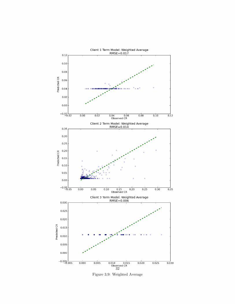
Figure 3.9: Weighted Average

32

Figure 3.10: KNN

33

Figure 3.11: Distance Weighted KNN

34

Figure 3.12: Random Forest

35

Figure 3.13: Combination: Weighted Average + Random Forest

36

3.4 Result Analysis

The results look very promising for Client 1 and 2, making very significantimprovements of the RMSE in both evaluation methods. The worse resultsof Client 3 is likely related to the smaller size of the data set and the datainjections. Client 3 also has a much more concentrated distribution of CRs,making the mean predictor perform much better than for other clients.

Unfortunately the term model suggested in this thesis relies on keywordswith more confident statistics to calculate the CR of keywords with no statistics.With no high traffic keywords in the data set it cannot perform well.

Considering how different the data looks for different clients it is not thatsurprising that certain models do better on some clients than others. The badlong tail results for Client 3 could very likely be due to that data set beingsignificantly smaller than other data sets.

Regarding the CTR model it should be noted that the test set containedonly keywords for which it is usable, but the keywords that are the primarytarget will not have as reliable statistics. For the term model however there isreason to believe it will add value to long tail keywords since it does not rely onanything other than the text in the keyword to make it’s predictions.

To give an idea of how the filtering skews the distribution of keywords Figure3.14 shows the number of keywords of different length before and after filtering.As shown in the figures the keywords that have enough conversions to be usedto test the model are not completely representative of the whole data set andsince they have statistics they would not be predicted using the models in thispaper. That being said there is still a fair amount of spread in the length of thekeywords.

37

Figure 3.14: Keyword length distributions

38

Chapter 4

Future Improvements

There is quite a lot of room for improvements of the results. The results in thispaper were calculated on criterion text, which is the text in the keyword. Thekeyword also has a match type which was not part of the data sets used here.There are three types of match types: Exact, Phrase and Broad. Exact matchonly matches searches equal to the criterion text, phrase match matches searchescontaining all the words and broad match searches that Google consider to besimilar. The exact search query can be attained and used to calculate the wordstatistics, in which case the model would make use of the extra informationgained by using broad match keywords. Calculating the statistics using searchqueries and including match type in the model would most likely improve theresult.

As of now the term models work only with words but it would require littlework to switch to a true term model, where combinations of words that appeartogether often will be treated as a one term. This would provide the algorithmswith a way to distinguish terms such as “free trial” from other uses of the word“free”, which could prove valuable.

Another thing that should be investigated is if the performance can be im-proved by treating branding keywords differently. The easiest way to accomplishthis would be not to include them when calculating the statistics for the termmodel, since branding traffic usually contains few long tail keywords anyway.

Also, if used in production this model should not be used on it’s own exceptwhen setting the first bid since it does not take the statistics for the keywordinto account.

39

Chapter 5

Critical Analysis

During the development of this prototype I made a few time consuming mistakes.The first being a bad choice of method to import the data, leaving me with aslow implementation which I ended up rewriting using the excellent Pandaslibrary.

The second implementation mistake was using CR′ ≈ 1+Conversions1+Clicks as an

approximation of CR to avoid division by zero. I did this before I came up withthe term model and stuck with it, only to realize later on that I didn’t need itanymore and the only effect it had was making the data less correct.

I also had no good benchmark on the performance. I would have liked tocompare it to Campanja’s current system but that could not be done. I endedup using the mean CR for each client as a benchmark and learned later thatthis is not a fair comparison of the current system’s performance.

The injected data into the data sets adds uncertainty to the results as well.I also made the mistake of using an approximation of CR, CR′ ≈ 1+Conversions

1+Clicks ,to avoid division by zero. The problem with this is that it skews the values whereConversions ≈ 0 making them useless anyway.

40

Bibliography

[1] python.org

[2] numpy.org

[3] pandas.pydata.org

[4] matplotlib.org

[5] scikit-learn.org

[6] orange.biolab.si

[7] Stokastik, Sven Erick Alm & Tom Britton, Liber, 2008

[8] Bayesian Reasoning and machine learning, David Barber, CambridgeUniversity Press, 2012

[9] A New Distance-weighted k-nearest Neighbor Classifier, Journal of In-formation & Computational Science 9:6 (2012)

[10] Random Forests, Leo Breiman, 2001,http://oz.berkeley.edu/ breiman/randomforest2001.pdf

[11] Data Mining - Practical Machine Learning Tools and Techniques, Thirdedition, Ian H. Witten, Eibe Frank, Mark A. Hall, Morgan Kaufmann,2011

41