precise study of the atmospheric neutrino …
TRANSCRIPT

BOSTON UNIVERSITY
GRADUATE SCHOOL OF ARTS AND SCIENCES
Dissertation
PRECISE STUDY OF THE ATMOSPHERIC NEUTRINO
OSCILLATION PATTERN USING SUPER-KAMIOKANDE I AND II
by
FANNY MAUDE DUFOUR
B.S., Universite libre de Bruxelles, 2003
Submitted in partial fulfillment of the
requirements for the degree of
Doctor of Philosophy
2009

Approved by
First ReaderEdward T. Kearns, Ph.D.Professor of Physics
Second ReaderTulika Bose, Ph.D.Assistant Professor of Physics

Acknowledgments
I would like to thank my parents and my brother for their support, and for not
complaining too much about the fact that I came to study particle physics in the US, on
a detector located in Japan, while I was born 30 km away from CERN. Then of course
I want to thank Vishal for his love and endless support.
The BU physics grad students made life in Boston real treat. The Friday nights
at The Other Side, the parties at Silvia, Jason, Claudio and countless others, and the
summer trips to Singing Beach; all these moments were vital to my mental health. I also
want to thank my friends in Switzerland, Anouk, Manu et les autres.. pour vos emails,
vos lettres, votre accueil pendant mes vacances, et le fait qu’apres onze ans d’absence
nous sommes toujours si proches.
My friends on the second floor of PRB deserve a special acknowledgment: Jason
for making my cubicle less dull once in a while, Jen for teaching me emacs keyboard
shortcuts and how to knit, Mike for teaching me the rules of baseball during the 2003
post-season so that I could enjoy 2004, Dan for hanging out at ERC in the morning, Wei
for giving me PC reduction, and Brian, for making PRB 268 less lonely after everybody
had moved to the lab or to Geneva. Thank you to Mirtha Cabello, superwoman to all
grad students in Physics at BU.
Naturally, not much of this thesis would have been achieved without the help of my
advisor, Ed Kearns. Thanks for teaching us how to present good talks and teaching all
of us to become better physicists. Many thanks to my committee members for their
time and comments: Tulika Bose, Lee Roberts, Sheldon Glashow and Anders Sandvik.
Finally, I wanted to thank our colleagues in the US and in Japan, Kate Scholberg, Roger
Wendell, Naho Tanimoto, Shigetaka Moriyama, Takaaki Kajita for their help inside and
outside Mozumi. And a special thanks to Piotr for taking over PC reduction!
iii

PRECISE STUDY OF THE ATMOSPHERIC NEUTRINO
OSCILLATION PATTERN USING SUPER-KAMIOKANDE I AND II
(Order No. )
FANNY DUFOUR
Boston University Graduate School of Arts and Sciences, 2009
Major Professor: Edward T. Kearns, Professor of Physics
ABSTRACT
Neutrino oscillation arises because the mass eigenstates of neutrinos are not identical
to the flavor eigenstates, and it is described by the PMNS (Pontecorvo, Maki, Naka-
gawa and Sakata) flavor mixing matrix. This matrix contains 6 parameters: 3 angles,
2 mass splittings and one CP violating phase. Using the atmospheric neutrino data
collected by the Super-Kamiokande water Cherenkov detector, we can measure two of
these parameters, ∆m223 and sin2 2θ23, which govern the oscillation of νµ → ντ .
The L/E analysis studies the ratio of flight length (L) to energy (E) and is the only
analysis which is able to resolve the expected oscillatory pattern of the survival proba-
bility: P (νµ → νµ) = 1− sin2(2θ)× sin2(1.27×∆m2 L(km)
E(GeV )
). To observe this oscillation
pattern, we divide the L/E distribution of muon neutrino data by a normalized un-
oscillated set of Monte Carlo. Events used in this analysis need good flight length and
energy resolution, therefore strict resolution cuts are applied. Hence, the data sample is
smaller than the sample used in the other Super-Kamiokande analysis [1]. Despite the
smaller sample, the L/E analysis gives a stronger constraint on ∆m223.
This thesis covers the L/E analysis of the Super-Kamiokande atmospheric data
collected during the Super-Kamiokande I (SK1: 1996-2001, 1489 days) and Super-
Kamiokande II (SK2: 2003-2005, 804 days) data-taking periods. The final values of the
oscillation parameters for the combined SK1+SK2 datasets, at 90% confidence level,
are sin2 2θ23 > 0.94 and 1.85× 10⁻³ eV 2 < ∆m223 < 2.65× 10⁻³ eV 2. The χ2 obtained
iv

with the oscillation hypothesis is lower than when we assume other models like neutrino
decay (3.7σ) or neutrino decoherence (4.7σ).
A significant part of this work was the improvement of the partially contained (PC)
event sample. This sample consists of neutrino events in which the outgoing charged
lepton exits the inner detector and deposits energy in the outer detector. These events
are very valuable to the L/E analysis because of their good flight length resolution. The
selection of PC events was improved from an 85% selection efficiency to a 97% efficiency
for the Super-Kamiokande III (SK3: 2006-2008, 526 days) dataset which will be used in
future analyses.
v

Preface
About sixty billion through one’s thumb every second.
The history of the solar neutrino problem is one of the most inspiring episodes of
particle physics. It is the story of a theorist, John Bahcall, an experimentalist Ray
Davis and the Homestake experiment which had been off by a factor of three for twenty-
four years. For twenty-four years, theorists and experimentalists worked to resolve this
discrepancy. The physics community considered that getting as close as a factor of
three was an achievement in itself, given the difficulty of the task. The factor of three
was probably just a little fluke somewhere. But both protagonists were convinced that
they were exactly right, not right up to a little fluke! The work continued until the
idea of neutrino oscillation presented by Pontecorvo, Maki, Nakagawa and Sakata [2, 3]
was being given a second chance. It allowed both the solar neutrino flux theoretical
calculation and the observation to be correct at the same time.
The Kamiokande experiment was first designed to look for proton decay. As you
well know, proton decay was never found. But the solar neutrino flux was measured
and was consistent with the Homestake experiment result. In addition, the atmospheric
neutrino flux was also measured, and as in the case of the solar neutrino flux, the theory
and the measurement were off by some factor. The neutrino oscillation model had just
been given another push.
In order to try to solve once and for all this discrepancy, Super-Kamiokande was
designed, and started operating in 1996. Two years later, neutrino oscillation was dis-

covered in both solar and atmospheric neutrino. The thirty years old disagreement
between a theorist and an experimentalist had produced two winners, and an inspiring
story about patience and hard work to the freshman physics student that I was then.
vii

Contents
Acknowledgments iii
Abstract iv
Foreword vi
Table of Contents viii
List of Tables xiii
List of Figures xv
List of Abbreviations xix
1 Introduction 1
2 Neutrino Theory 5
2.1 The mass of the neutrino . . . . . . . . . . . . . . . . . . . . . . . . . . . 5
2.2 Neutrino oscillation . . . . . . . . . . . . . . . . . . . . . . . . . . . . . . 8
2.3 Importance of precise θ23 and ∆m223 measurement . . . . . . . . . . . . . 11
2.4 Remaining open questions . . . . . . . . . . . . . . . . . . . . . . . . . . 12
3 Other neutrino oscillation experiments 14
3.1 Solar neutrinos θ12: Homestake, Kamiokande, IMB, SNO, Borexino . . . 15
viii

3.2 KamLAND (∆m212) and Chooz (θ13) . . . . . . . . . . . . . . . . . . . . 16
3.3 K2K and MINOS . . . . . . . . . . . . . . . . . . . . . . . . . . . . . . . 16
3.4 Current neutrino oscillation results . . . . . . . . . . . . . . . . . . . . . 17
4 The Super-Kamiokande Detector 21
4.1 Cherenkov effect . . . . . . . . . . . . . . . . . . . . . . . . . . . . . . . 21
4.2 Overview of the detector . . . . . . . . . . . . . . . . . . . . . . . . . . . 23
4.2.1 History of the Super-Kamiokande detector and differences in the
detector between each data-taking period . . . . . . . . . . . . . . 25
4.2.2 Description of the PMTs . . . . . . . . . . . . . . . . . . . . . . . 27
4.3 Overview of electronics and DAQ . . . . . . . . . . . . . . . . . . . . . . 30
4.3.1 ID electronics and DAQ . . . . . . . . . . . . . . . . . . . . . . . 30
4.3.2 OD electronics and DAQ . . . . . . . . . . . . . . . . . . . . . . . 32
4.3.3 Trigger . . . . . . . . . . . . . . . . . . . . . . . . . . . . . . . . . 33
4.4 Radon hut and water purification . . . . . . . . . . . . . . . . . . . . . . 34
4.5 Calibration . . . . . . . . . . . . . . . . . . . . . . . . . . . . . . . . . . 34
5 Simulation 38
5.1 Atmospheric neutrino flux . . . . . . . . . . . . . . . . . . . . . . . . . . 38
5.2 Neutrino interaction . . . . . . . . . . . . . . . . . . . . . . . . . . . . . 42
5.2.1 Elastic and quasi-elastic scattering . . . . . . . . . . . . . . . . . 43
5.2.2 Single meson production . . . . . . . . . . . . . . . . . . . . . . . 45
5.2.3 Deep inelastic scattering . . . . . . . . . . . . . . . . . . . . . . . 45
5.2.4 Coherent pion production . . . . . . . . . . . . . . . . . . . . . . 46
5.2.5 Nuclear effects . . . . . . . . . . . . . . . . . . . . . . . . . . . . . 47
5.3 Detector simulation . . . . . . . . . . . . . . . . . . . . . . . . . . . . . . 49
6 Data Reduction 50
ix

6.1 Fully-contained reduction . . . . . . . . . . . . . . . . . . . . . . . . . . 51
6.1.1 First reduction . . . . . . . . . . . . . . . . . . . . . . . . . . . . 51
6.1.2 Second reduction . . . . . . . . . . . . . . . . . . . . . . . . . . . 52
6.1.3 Third reduction . . . . . . . . . . . . . . . . . . . . . . . . . . . . 52
6.1.4 Fourth reduction . . . . . . . . . . . . . . . . . . . . . . . . . . . 55
6.1.5 Fifth reduction . . . . . . . . . . . . . . . . . . . . . . . . . . . . 55
6.1.6 Final FC cuts . . . . . . . . . . . . . . . . . . . . . . . . . . . . . 57
6.1.7 Status for SK1 and SK2 datasets . . . . . . . . . . . . . . . . . . 58
6.2 Partially-contained reduction . . . . . . . . . . . . . . . . . . . . . . . . 59
6.2.1 First reduction . . . . . . . . . . . . . . . . . . . . . . . . . . . . 59
6.2.2 Second reduction . . . . . . . . . . . . . . . . . . . . . . . . . . . 59
6.2.3 Third reduction . . . . . . . . . . . . . . . . . . . . . . . . . . . . 61
6.2.4 Fourth reduction . . . . . . . . . . . . . . . . . . . . . . . . . . . 61
6.2.5 Fifth reduction . . . . . . . . . . . . . . . . . . . . . . . . . . . . 62
6.2.6 Status for SK1 and SK2 datasets . . . . . . . . . . . . . . . . . 66
7 Data Reconstruction 67
7.1 Vertex fitting (tfafit) . . . . . . . . . . . . . . . . . . . . . . . . . . . . 67
7.1.1 Point fit (pfit) . . . . . . . . . . . . . . . . . . . . . . . . . . . . 67
7.1.2 Ring edge search . . . . . . . . . . . . . . . . . . . . . . . . . . . 68
7.1.3 TDC-fit (tftdcfit) . . . . . . . . . . . . . . . . . . . . . . . . . 69
7.2 Ring counting (rirngcnt) . . . . . . . . . . . . . . . . . . . . . . . . . . 70
7.2.1 Ring candidate search . . . . . . . . . . . . . . . . . . . . . . . . 70
7.2.2 Ring candidate test . . . . . . . . . . . . . . . . . . . . . . . . . . 72
7.3 Particle Identification (sppatid) . . . . . . . . . . . . . . . . . . . . . . . 73
7.3.1 Expected charge distributions . . . . . . . . . . . . . . . . . . . . 74
7.3.2 Estimation of particle type . . . . . . . . . . . . . . . . . . . . . . 75
x

7.4 Precise vertex fitting . . . . . . . . . . . . . . . . . . . . . . . . . . . . . 77
7.5 Momentum determination (spfinalsep) . . . . . . . . . . . . . . . . . . 78
7.6 Ring number correction (aprngcorr) . . . . . . . . . . . . . . . . . . . . 79
8 Dataset 83
8.1 Events samples . . . . . . . . . . . . . . . . . . . . . . . . . . . . . . . . 84
8.1.1 FC single-ring and multi-ring . . . . . . . . . . . . . . . . . . . . 84
8.1.2 PC stopping and through-going . . . . . . . . . . . . . . . . . . . 85
8.2 Reconstructing L and E . . . . . . . . . . . . . . . . . . . . . . . . . . . 87
8.2.1 Energy . . . . . . . . . . . . . . . . . . . . . . . . . . . . . . . . . 87
8.2.2 Flight Length . . . . . . . . . . . . . . . . . . . . . . . . . . . . . 90
8.3 Resolution cut . . . . . . . . . . . . . . . . . . . . . . . . . . . . . . . . . 95
8.4 Event summary . . . . . . . . . . . . . . . . . . . . . . . . . . . . . . . . 96
9 L/E analysis 101
9.1 Maximum likelihood analysis and χ2 fit . . . . . . . . . . . . . . . . . . . 102
9.1.1 Combining SK1 and SK2 dataset . . . . . . . . . . . . . . . . . . 104
9.2 Systematic uncertainties . . . . . . . . . . . . . . . . . . . . . . . . . . . 105
9.2.1 Simulation uncertainties - Neutrino flux . . . . . . . . . . . . . . 105
9.2.2 Simulation uncertainties - Neutrino Interactions . . . . . . . . . . 110
9.2.3 Reconstruction uncertainties . . . . . . . . . . . . . . . . . . . . . 110
9.2.4 Reduction uncertainties . . . . . . . . . . . . . . . . . . . . . . . 113
9.3 Results . . . . . . . . . . . . . . . . . . . . . . . . . . . . . . . . . . . . . 115
9.3.1 Dealing with non physical region . . . . . . . . . . . . . . . . . . 115
9.3.2 Oscillation results . . . . . . . . . . . . . . . . . . . . . . . . . . . 115
9.3.3 Neutrino decoherence and decay . . . . . . . . . . . . . . . . . . . 117
9.3.4 Neutrino Decay . . . . . . . . . . . . . . . . . . . . . . . . . . . . 119
9.3.5 Neutrino Decoherence . . . . . . . . . . . . . . . . . . . . . . . . 121
xi

10 Conclusion 122
A Partially contained data reduction 125
A.1 Purpose of the OD segmentation added for SK3 . . . . . . . . . . . . . . 125
A.2 Modifications to PC reduction for SK3 . . . . . . . . . . . . . . . . . . . 126
A.3 New PC reduction results . . . . . . . . . . . . . . . . . . . . . . . . . . 131
A.4 PC reduction systematics uncertainty . . . . . . . . . . . . . . . . . . . . 132
B Distributions of reconstructed variables 136
B.1 Vertex distributions . . . . . . . . . . . . . . . . . . . . . . . . . . . . . . 136
B.2 Number of ring distributions . . . . . . . . . . . . . . . . . . . . . . . . . 137
B.3 PID distributions . . . . . . . . . . . . . . . . . . . . . . . . . . . . . . . 138
C Proof that binned and unbinned likelihood are equivalent 145
D Use of a fully reconstructed charged current quasi-elastic (CCQE) sam-
ple 148
D.1 Selecting the CCQE sample . . . . . . . . . . . . . . . . . . . . . . . . . 149
D.2 Energy and flight length reconstruction for the CCQE sample . . . . . . 150
D.3 Statistics of the CCQE sample . . . . . . . . . . . . . . . . . . . . . . . . 151
D.4 Testing the sensitivity of the CCQE sample . . . . . . . . . . . . . . . . 154
List of Journal Abbreviation 157
Bibliography 158
Curriculum Vitae 164
xii

List of Tables
2.1 Dirac lepton states . . . . . . . . . . . . . . . . . . . . . . . . . . . . . . 7
3.1 Current status of oscillation parameter measurements (Ref.[4]). . . . . . 17
4.1 Summary of differences between the SK1, SK2 and SK3 data-taking periods 27
4.2 Hamamatsu R1408 and R5912 . . . . . . . . . . . . . . . . . . . . . . . . 29
5.1 List of processes considered in the GEANT simulation. . . . . . . . . . . 49
6.1 SK1 and SK2 FC reduction summary. . . . . . . . . . . . . . . . . . . . 58
6.2 SK1 and SK2 FC background contamination upper limits. . . . . . . . . 58
6.3 SK1 and SK2 PC reduction summary. . . . . . . . . . . . . . . . . . . . . 66
7.1 Vertex resolution and angular resolution for SK1 and SK2. . . . . . . . . 77
8.1 Summary of the event samples for SK1 and SK2 data. . . . . . . . . . . . 99
9.1 Schematic view of the fij matrix modified to account for two datasets . . 105
9.2 Systematic uncertainties - Neutrino flux . . . . . . . . . . . . . . . . . . 106
9.3 Systematic uncertainties - Neutrino interaction . . . . . . . . . . . . . . 107
9.4 Systematic uncertainties - Reconstruction and Reduction . . . . . . . . . 108
A.1 PC reduction efficiencies for old and new PC reduction . . . . . . . . . . 132
A.2 SK-III Dataset for 551 days of data . . . . . . . . . . . . . . . . . . . . . 132
xiii

D.1 CCQE sample statistics . . . . . . . . . . . . . . . . . . . . . . . . . . . 154
xiv

List of Figures
1.1 Pauli’s letter . . . . . . . . . . . . . . . . . . . . . . . . . . . . . . . . . . 2
1.2 Survival probability of νµ → νµ . . . . . . . . . . . . . . . . . . . . . . . 3
2.1 Dirac mass term for an electron. . . . . . . . . . . . . . . . . . . . . . . . 6
2.2 Dirac mass term for neutrino. . . . . . . . . . . . . . . . . . . . . . . . . 7
2.3 Majorana mass term for neutrino. . . . . . . . . . . . . . . . . . . . . . . 8
2.4 Schematic of the seesaw mechanism. . . . . . . . . . . . . . . . . . . . . . 9
3.1 Global fit for 1-2 sector . . . . . . . . . . . . . . . . . . . . . . . . . . . . 18
3.2 Global fit for 2-3 sector . . . . . . . . . . . . . . . . . . . . . . . . . . . . 19
3.3 Global fit for 1-3 sector . . . . . . . . . . . . . . . . . . . . . . . . . . . . 20
4.1 Example of Cherenkov muon ring . . . . . . . . . . . . . . . . . . . . . . 22
4.2 Schematic view of the Super-Kamiokande detector [5]. . . . . . . . . . . 23
4.3 Details of the stainless steel structure, and mounting of the PMT [5]. . . 24
4.4 Veto counters . . . . . . . . . . . . . . . . . . . . . . . . . . . . . . . . . 25
4.5 20 inch PMT in its acrylic shell. Shell was added after SK1. . . . . . . . 26
4.6 Old (red empty squares) and new (full black square) PMTs for the SK2
period. The SK1 period uses only old tubes, and the SK3 period is very
similar to SK2. . . . . . . . . . . . . . . . . . . . . . . . . . . . . . . . . 27
4.7 Schematic of a 20 inch ID PMT [5]. . . . . . . . . . . . . . . . . . . . . . 28
4.8 Schematic of an 8 inch R5912 OD PMT . . . . . . . . . . . . . . . . . . 29
xv

4.9 Quantum efficiency for R1408 and R5912 . . . . . . . . . . . . . . . . . . 30
4.10 A schematic view of the analog input block of the ATM . . . . . . . . . . 31
4.11 The ID data acquisition system [5]. . . . . . . . . . . . . . . . . . . . . . 32
4.12 Linac system . . . . . . . . . . . . . . . . . . . . . . . . . . . . . . . . . 35
4.13 Energy calibration . . . . . . . . . . . . . . . . . . . . . . . . . . . . . . 37
5.1 Atmospheric neutrino flux and the flavor ratio . . . . . . . . . . . . . . . 40
5.2 Example of 1D versus 3D flux calculation . . . . . . . . . . . . . . . . . . 41
5.3 Neutrino production height . . . . . . . . . . . . . . . . . . . . . . . . . 42
5.4 Quasi-elastic cross-sections . . . . . . . . . . . . . . . . . . . . . . . . . . 44
5.5 Single π charged current cross-sections (νµ) . . . . . . . . . . . . . . . . . 46
5.6 Single π charged current cross-sections (νµ) . . . . . . . . . . . . . . . . . 47
5.7 Deep inelastic cross-sections . . . . . . . . . . . . . . . . . . . . . . . . . 48
5.8 Coherent pions cross sections . . . . . . . . . . . . . . . . . . . . . . . . 48
6.1 Schematic view of different event samples. . . . . . . . . . . . . . . . . . 51
6.2 Number of hits in the OD endcaps versus in the OD wall . . . . . . . . . 60
7.1 Example of (PE(θ)) and its second derivative . . . . . . . . . . . . . . . 69
7.2 Schematic view of a Hough transform for a radius of 42 [6]. . . . . . . . 71
7.3 Map of Hough transform . . . . . . . . . . . . . . . . . . . . . . . . . . . 71
7.4 Ring counting likelihood for SK1 and SK2 . . . . . . . . . . . . . . . . . 72
7.5 Example 1 GeV muon and 1 GeV electron . . . . . . . . . . . . . . . . . 73
7.6 Vertex resolution for SK1 . . . . . . . . . . . . . . . . . . . . . . . . . . 78
7.7 Vertex resolution for SK2 . . . . . . . . . . . . . . . . . . . . . . . . . . 79
7.8 Angular resolution for SK1 . . . . . . . . . . . . . . . . . . . . . . . . . . 80
7.9 Angular resolution for SK2 . . . . . . . . . . . . . . . . . . . . . . . . . . 81
7.10 Momentum resolution . . . . . . . . . . . . . . . . . . . . . . . . . . . . 82
xvi

8.1 Separation criteria between PC OD stopping and PC OD through-going
events . . . . . . . . . . . . . . . . . . . . . . . . . . . . . . . . . . . . . 87
8.2 Pµ/Dinner distributions for PC single-ring events. . . . . . . . . . . . . . 89
8.3 (Etrueν − Erec
ν )/Etrueν distributions for SK1 . . . . . . . . . . . . . . . . . 91
8.4 (Etrueν − Erec
ν )/Etrueν distributions for SK2 . . . . . . . . . . . . . . . . . 92
8.5 Energy resolution for SK1 (left) and SK2 (right). . . . . . . . . . . . . . 92
8.6 Angle between true and reconstructed neutrino direction for SK1 . . . . 93
8.7 Angle between true and reconstructed neutrino direction for SK2 . . . . 94
8.8 Angular resolution for SK1 (left) and SK2 (right). . . . . . . . . . . . . . 94
8.9 True flight length versus true zenith angle . . . . . . . . . . . . . . . . . 95
8.10 Resolution maps . . . . . . . . . . . . . . . . . . . . . . . . . . . . . . . 97
8.11 Effect of resolution cuts . . . . . . . . . . . . . . . . . . . . . . . . . . . 98
8.12 Effect of the resolution cut . . . . . . . . . . . . . . . . . . . . . . . . . . 98
8.13 Stacked L/E distribution for each sub-sample . . . . . . . . . . . . . . . 100
9.1 Survival probability of νµ → ντ . . . . . . . . . . . . . . . . . . . . . . . 101
9.2 Energy calibration . . . . . . . . . . . . . . . . . . . . . . . . . . . . . . 112
9.3 Energy calibration (up-down) . . . . . . . . . . . . . . . . . . . . . . . . 113
9.4 PEanti/PEexp for SK1 barrel . . . . . . . . . . . . . . . . . . . . . . . . . 114
9.5 1996 PDG method to treat results close to physical boundary . . . . . . 116
9.6 L/E spectrum . . . . . . . . . . . . . . . . . . . . . . . . . . . . . . . . . 117
9.7 Theoretical survival probability and Experimental survival probability . . 118
9.8 Contour map of the oscillation analysis for the SK1 + SK2 dataset. . . . 119
9.9 Left: Slice in ∆m223. Right: in sin2 2θ23. . . . . . . . . . . . . . . . . . . . 119
9.10 Survival probability and best fit results . . . . . . . . . . . . . . . . . . . 120
10.1 Experimental survival probability . . . . . . . . . . . . . . . . . . . . . . 122
10.2 90% CL contours for SK L/E, SK zenith, and MINOS . . . . . . . . . . 124
xvii

A.1 Schematic view of the OD segmentation (red lines) added in SK3 . . . . 126
A.2 Number of hits in the OD wall versus in the OD end-caps . . . . . . . . . 127
A.3 Event rate for PC SK3 . . . . . . . . . . . . . . . . . . . . . . . . . . . . 133
A.4 Zenith angle for PC SK3 . . . . . . . . . . . . . . . . . . . . . . . . . . . 134
A.5 Distance to the wall (cm) for BG events accepted by PC reduction. The
green shaded area contains events which are added when we remove the
corner cut in PC5. . . . . . . . . . . . . . . . . . . . . . . . . . . . . . 135
B.1 Vertex distributions for SK1 (Z) . . . . . . . . . . . . . . . . . . . . . . 137
B.2 Vertex distributions for SK1 (R2) . . . . . . . . . . . . . . . . . . . . . . 138
B.3 Vertex distributions for SK2 (Z) . . . . . . . . . . . . . . . . . . . . . . 139
B.4 Vertex distributions for SK2 (R2) . . . . . . . . . . . . . . . . . . . . . . 140
B.5 Number of rings distributions for SK1. . . . . . . . . . . . . . . . . . . . 141
B.6 Number of rings distributions for SK2. . . . . . . . . . . . . . . . . . . . 142
B.7 PID likelihood distributions for SK1. . . . . . . . . . . . . . . . . . . . . 143
B.8 PID likelihood distributions for SK2. . . . . . . . . . . . . . . . . . . . . 144
D.1 Reconstructed versus true energy and flight length for events identified
as CCQE . . . . . . . . . . . . . . . . . . . . . . . . . . . . . . . . . . . 152
D.2 Reconstructed L/E bin versus true L/E bin for events identified as CCQE153
D.3 Example of fake dataset . . . . . . . . . . . . . . . . . . . . . . . . . . . 155
D.4 Results of adding CCQE sample . . . . . . . . . . . . . . . . . . . . . . . 156
xviii
List of Abbreviations
ADC . . . . . . . . . . . . . . . . . . . . . . . . . . . . . . . . . . . . . . . . . . . . . . . . . . . . Analog to Digital Converter
ATM . . . . . . . . . . . . . . . . . . . . . . . . . . . . . . . . . . . . . . . . . . . . . . . . . . . . . . . . . Analog Timing Module
BG . . . . . . . . . . . . . . . . . . . . . . . . . . . . . . . . . . . . . . . . . . . . . . . . . . . . . . . . . . . . . . . . . . . . . . Background
CC . . . . . . . . . . . . . . . . . . . . . . . . . . . . . . . . . . . . . . . . . . . . . . . . . . . . . . . . . . . . . . . . . Charged Current
CCD . . . . . . . . . . . . . . . . . . . . . . . . . . . . . . . . . . . . . . . . . . . . . . . . . . . . . . . . . Charge-Coupled Device
CCQE . . . . . . . . . . . . . . . . . . . . . . . . . . . . . . . . . . . . . . . . . . . . . . . . Charged Current Quasi-Elastic
CL . . . . . . . . . . . . . . . . . . . . . . . . . . . . . . . . . . . . . . . . . . . . . . . . . . . . . . . . . . . . . . . . . Confidence Level
DAQ . . . . . . . . . . . . . . . . . . . . . . . . . . . . . . . . . . . . . . . . . . . . . . . . . . . . . . . . . . . . . . . Data Acquisition
DIS . . . . . . . . . . . . . . . . . . . . . . . . . . . . . . . . . . . . . . . . . . . . . . . . . . . . . . . . .Deep Inelastic Scattering
EM . . . . . . . . . . . . . . . . . . . . . . . . . . . . . . . . . . . . . . . . . . . . . . . . . . . . . . . . . . . . . . . .Electromagnetism
FRP . . . . . . . . . . . . . . . . . . . . . . . . . . . . . . . . . . . . . . . . . . . . . . . . . . . . . . . . Fiber-Reinforced Plastic
GONG . . . . . . . . . . . . . . . . . . . . . . . . . . . . . . . . . . . . . . . . . . . . . . . . . . . . . . . . . . . . . . . . . . . . GO-NoGo
GUT . . . . . . . . . . . . . . . . . . . . . . . . . . . . . . . . . . . . . . . . . . . . . . . . . . . . . . . . . . Grand Unified Theory
ID . . . . . . . . . . . . . . . . . . . . . . . . . . . . . . . . . . . . . . . . . . . . . . . . . . . . . . . . . . . . . . . . . . . . Inner Detector
IMB . . . . . . . . . . . . . . . . . . . . . . . . . . . . . . . . . . . . . . . . . . . . . . . . . . . . .Irvine Michigan Brookhaven
KAMLAND . . . . . . . . . . . . . . . . . . . . . Kamioka Liquid Scintillator Anti-Neutrino Detector
LHC . . . . . . . . . . . . . . . . . . . . . . . . . . . . . . . . . . . . . . . . . . . . . . . . . . . . . . . . . . Large Hadron Collider
LINAC . . . . . . . . . . . . . . . . . . . . . . . . . . . . . . . . . . . . . . . . . . . . . . . . . . . . . . . . . . . .Linear Accelerator
MC . . . . . . . . . . . . . . . . . . . . . . . . . . . . . . . . . . . . . . . . . . . . . . . . . . . . . . . . . . . . . . . . . . . . . Monte Carlo
MS-fit . . . . . . . . . . . . . . . . . . . . . . . . . . . . . . . . . . . . . . . . . . . . . . . . . . . . . . . . . . . Muon-Shower Fitter
NC . . . . . . . . . . . . . . . . . . . . . . . . . . . . . . . . . . . . . . . . . . . . . . . . . . . . . . . . . . . . . . . . . . Neutral Current
OD . . . . . . . . . . . . . . . . . . . . . . . . . . . . . . . . . . . . . . . . . . . . . . . . . . . . . . . . . . . . . . . . . . .Outer Detector
PDF . . . . . . . . . . . . . . . . . . . . . . . . . . . . . . . . . . . . . . . . . . . . . . . . . . . .Probability Density Function
PE . . . . . . . . . . . . . . . . . . . . . . . . . . . . . . . . . . . . . . . . . . . . . . . . . . . . . . . . . . . . . . . . . . . Photoelectrons
PID . . . . . . . . . . . . . . . . . . . . . . . . . . . . . . . . . . . . . . . . . . . . . . . . . . . . . . . . . . . .Particle identification
xix

PMT . . . . . . . . . . . . . . . . . . . . . . . . . . . . . . . . . . . . . . . . . . . . . . . . . . . . . . . . . . . Photomultiplier tube
QAC . . . . . . . . . . . . . . . . . . . . . . . . . . . . . . . . . . . . . . . . . . . . . . . . . . . . Charge-to-Analog Converter
QE . . . . . . . . . . . . . . . . . . . . . . . . . . . . . . . . . . . . . . . . . . . . . . . . . . . . . . . . . . . . . . . . . . . . .Quasi-Elastic
QTC . . . . . . . . . . . . . . . . . . . . . . . . . . . . . . . . . . . . . . . . . . . . . . . . . . . . . . Charge-to-Time Converter
SK . . . . . . . . . . . . . . . . . . . . . . . . . . . . . . . . . . . . . . . . . . . . . . . . . . . . . . . . . . . . . . . Super-Kamiokande
SK1 . . . . . . . . . . . . . . . . . . . . . . . . . . . . . . . . . . . . . . . . . . . . . . . . . . . . . . . . . . . . .Super-Kamiokande I
SK2 . . . . . . . . . . . . . . . . . . . . . . . . . . . . . . . . . . . . . . . . . . . . . . . . . . . . . . . . . . . . Super-Kamiokande II
SK3 . . . . . . . . . . . . . . . . . . . . . . . . . . . . . . . . . . . . . . . . . . . . . . . . . . . . . . . . . . . Super-Kamiokande III
SM . . . . . . . . . . . . . . . . . . . . . . . . . . . . . . . . . . . . . . . . . . . . . . . . . . . . . . . . . . . . . . . . . . Standard Model
SNO . . . . . . . . . . . . . . . . . . . . . . . . . . . . . . . . . . . . . . . . . . . . . . . . . .Sudbury Neutrino Observatory
Super-K . . . . . . . . . . . . . . . . . . . . . . . . . . . . . . . . . . . . . . . . . . . . . . . . . . . . . . . . . . Super-Kamiokande
TAC . . . . . . . . . . . . . . . . . . . . . . . . . . . . . . . . . . . . . . . . . . . . . . . . . . . . . . Time-to-Analog Converter
TDC . . . . . . . . . . . . . . . . . . . . . . . . . . . . . . . . . . . . . . . . . . . . . . . . . . . . . . Time-to-Digital Converter
TKO . . . . . . . . . . . . . . . . . . . . . . . . . . . . . . . . . . . . . . . . . . . . . . . . . . . . . . . . . . . . Tristan KEK Online
VME . . . . . . . . . . . . . . . . . . . . . . . . . . . . . . . . . . . . . . . . . . . . . . . . . . . . . . . . . . Versa Module Europa
xx

Chapter 1
Introduction
The neutrino was first introduced by Wolfgang Pauli in 1930 [7] to explain the continuous
β decay (n→ p+ e− + ν) spectrum and to conserve energy and momentum. When the
energy of the outgoing electron is measured, the result is a continuous spectrum. This
result would not conserve energy and momentum if β decay were a two-body decay.
Pauli’s solution was to introduce a nearly massless neutral particle to make β decay a
three-body decay. Pauli announced his idea in a letter and a translation of his letter is
shown in Fig. 1.1.
Two decades after this first proposal, in 1956, Reines and Cowan [8] were able to
observe neutrinos for the first time through an inverse β decay process: νe+p→ n+e+.
Ten years later, in 1962, Lederman, Schwartz and Steinberger [9] discovered the muon
neutrino, through the decay of the pion (π → µ+ νµ). And finally in 2000 at Fermilab,
the expected τ neutrino was observed by the DONUT experiment [10], 25 years after
the discovery of the τ lepton.
In the 1970’s, the Homestake experiment [11] measured the solar neutrino flux and its
result disagreed with the solar neutrino flux calculation done by John Bahcall [12]. This
was called the “solar neutrino problem” and it was the first hint that neutrinos might
oscillate, as proposed earlier by Maki, Nakagawa and Sakata in 1962 [2] and Pontecorvo
in 1968 [3].
1

2
Figure 1.1: Translation of Pauli’s famous letter about his proposal of neutrinos (calledneutrons in the letter) [7]
In the 1980’s several experiments were built to study solar and atmospheric neutrinos.
Kamiokande [13] in Japan, and IMB [14] in the United States. In addition studying solar
and atmospheric neutrinos, both detectors were able to observe neutrinos coming from
the supernova SN1987A. These neutrinos are the only extra-galactic neutrinos observed
so far.
In 1998, when the Super-Kamiokande collaboration presented its atmospheric neu-
trino data analysis showing a deficit of upward going muon neutrinos, the physics com-

3
Figure 1.2: Survival probability of νµ → νµ, without any detector effect as a function ofL/E.
munity was convinced that neutrino oscillation was the solution to the “solar neutrino
problem,” and explained the atmospheric neutrino data.
However, at this point, nobody had seen the oscillatory pattern predicted by the
theory. Only a deficit of upward-going neutrinos was observed and other theories like
neutrino decay or neutrino decoherence could explain the atmospheric neutrino data.
In the two flavor approximation, the survival probability of the muon neutrino is
written as: P (νµ → νµ) = 1− sin2(2θ23)× sin2(1.27×∆m2
23 ×L(km)E(GeV )
)and is shown in
Fig. 1.2.
Atmospheric neutrinos have a wide range of energies (E), from a few MeV to several
GeV, and a wide range of flight lengths (L) from about 10 km for downward-going neu-
trinos to about 10000 km for upward-going neutrinos. Thanks to these wide ranges in L
and E, we have access to neutrinos with a wide range of L/E values. Using atmospheric
muon neutrinos collected by the Super-Kamiokande detector, we can therefore directly
observe the oscillatory pattern of survival probability as a function of L/E as shown in
Fig. 1.2.

4
Because the energy and flight length resolutions are not perfect, the resulting L/E
resolution only allows us to see the first minimum in the survival probability and the rise
after this minimum before the oscillation pattern is no longer distinguishable and only
the average value of the survival probability is observed. The position of the minimum
is a direct measurement of ∆m223, and the level at which the probability averages out is
a measurement of sin2(2θ23).

Chapter 2
Neutrino Theory
For many years, neutrinos were assumed to be massless, but the observation of atmo-
spheric muon neutrino disappearance by the Super-Kamiokande collaboration in 1998 [1]
changed the game. Physicists were now seeing both atmospheric and solar neutrinos be-
having differently from what was expected. Neutrino oscillations could explain both the
solar and the atmospheric data, but these oscillations required neutrinos to be massive,
and that the mass eigenstates be different from the flavor eigenstates.
2.1 The mass of the neutrino
After the discovery of muon neutrino disappearance by the Super-Kamiokande experi-
ment, the most widely accepted explanation was neutrino oscillation. Since oscillation
is possible only with massive neutrino, it is interesting to study how the neutrino mass
term is introduced in the Standard Model. Usually, in the Standard Model, spin-1/2
particles acquire their mass through interaction with the Higgs background field, as
shown in Fig. 2.1.
These mass terms are called Dirac mass terms and are presented in Eq. 2.1. One of their
characteristics is that they change the handedness of particles; a left-handed electron
becomes a right-handed electron through its interaction with the Higgs field [15]:
5

6
Figure 2.1: Dirac mass term for an electron.
Lfermions = −Ge
(νe, e)L
h+
h0
eR + eR(h−, h0)
νe
e
L
, (2.1)
where Ge is an arbitrary Yukawa coupling that can be chosen to be me = Gev√2
, (νe, e)L, is
the weak isospin doublet, h is the Higgs doublet and er an isospin singlet. For massless
neutrinos, the Higgs doublet is rewritten as:
h =
√1
2
0
v + h(x)
, (2.2)
where v is the non-zero vacuum expectation value of the Higgs field. In the Standard
Model, the electron mass comes from the Yukawa coupling of the electron to the Higgs
vacuum expectation.
Dirac mass terms conserve electric charge, and they conserve lepton number; a par-
ticle does not become an anti-particle when it interacts with the vacuum expectation of
the Higgs field < h0 >= v√2. Dirac particles have four states, for example: eL, eR, eR
and eL. Only the first two states interact weakly and each are part of a weak isospin
doublet with its neutrino counterpart. The last two states are weak isospin singlets.
The Dirac states of leptons are summarized in Table 2.1.
So far we have seen only the left-handed neutrino and the right-handed anti-neutrino.
If neutrinos behave like all other spin-1/2 particles and are Dirac particles then two
new states need to be introduced: the right-handed neutrino and the left-handed anti-

7
Particle Handedness Particle Weak ElectricNumber States Isospin Charge
Charge+1+1
LL
(eLνL
)−1/2+1/2
−10
−1−1
RR
(eRνR
)+1/2−1/2
+10
+1 R eR 0 -1-1 L eL 0 +1+1 R νR 0 0-1 L νL 0 0
Table 2.1: Dirac lepton states
Figure 2.2: Dirac mass term for neutrino.
neutrino. These two states are called sterile, as they do not even interact weakly. In
that case the neutrinos would get their mass through the usual Higgs mechanism as
shown in Fig. 2.2. We use the process which gives mass to the upper member of the
quark doublet. With Dirac masses, nothing explains why the masses of the neutrinos
are so much smaller than the masses of their associated leptons.
As mentioned earlier, we have so far only observed two states of neutrinos, not four.
If we do not want to introduce the two extra states, then neutrinos cannot have Dirac
mass terms as this would violate the conservation of lepton number assumed for such
terms. But if we allow lepton number violation, the 2-state neutrinos can acquire mass
through the interaction with the Higgs background field as shown in Fig. 2.3. These are
Majorana mass terms and they change both handedness and lepton number. Since the
lagrangian density has units of E4, the fermion fields of E3/2 and the Higgs field of E1,

8
Figure 2.3: Majorana mass term for neutrino.
we can see that an energy scale needs to be introduced. Therefore, this is an effective
theory.
The most widely accepted explanation for this difference in masses is the seesaw
mechanism [16–19]. In that case, neutrinos have both Dirac and Majorana mass terms,
and they acquire their mass through their interaction with the Higgs field as shown
in Fig. 2.4. The coefficient of the Majorana mass term M can be very large, and the
coefficient of the Dirac mass term m can be of the order of the other lepton mass.
The neutrino would not have states of definite mass, but would split into two neutrinos
having a mass of m2/M and two neutrinos of mass M . This is explained in more details
in Ref. [20]. The very light neutrino would be mostly the left-handed neutrino and the
very heavy would be the sterile right-handed neutrino. Similarly, the very light anti-
neutrino would the right-handed one, the very heavy, the left-handed one. The feature
of a very light mass and a very heavy mass balancing each other is what gave its name
to the seesaw mechanism. (Reading “the oscillating neutrino” [21] was very helpful to
write this section.)
2.2 Neutrino oscillation
The idea that neutrinos oscillate was first proposed separately by Pontecorvo and by
Maki, Nakagawa and Sakata [2, 3]. In the 1960’s and was later a good explanation for the
disappearance of both solar and atmospheric neutrino observed by several experiments.

9
Figure 2.4: Schematic of the seesaw mechanism.
Neutrino oscillation relies on the fact that the mass eigenstates are not identical to the
flavor eigenstates. This is similar to what happens in the quark sector because of the
CKM matrix [22, 23], but in this case it involves the weak interaction instead of the
strong interaction. Mass and flavor eigenstates are related as in the following equation
by the PMNS matrix U, where Sij(Cij) stands for sin θij (cos θij), and δ is the CP
violating phase:
νe
νµ
ντ
=
Ue1 Ue2 Ue3
Uµ1 Uµ2 Uµ3
Uτ1 Uτ2 Uτ3
ν1
ν2
ν3
(2.3)
U =
1 0 0
0 C23 S23
0 −S23 C23
C13 0 S13e−iδ
0 1 0
−S13eiδ 0 C13
C12 S12 0
−S12 C12 0
0 0 1
(2.4)
As for all fermions and taking into account the PMNS matrix, the wave function of a
neutrino in the flavor eigenstate α can be written as:
Ψα(x, t) =∑i
Uαi exp−ipix νi =∑i
Uαi exp−iEit+ipνx νi. (2.5)
Since the masses of the neutrinos are very small, we know that Ei ≈ pν +m2i
2pνand

10
therefore:
Ψα(x, t) = expipν(x−t)(∑i
Uαi exp−im2i t
2pν )νi. (2.6)
Assuming that a neutrino of flavor α is traveling at the speed of light c for a distance
L, we can write its probability to be in a flavor eigenstate β at time t as:
P (να → νβ) = |∑i
UαiU∗iβ exp−
im2i t
2pν |2
=∑i
|UαiU∗iβ|2 +Re∑i
∑i 6=j
UαiU∗iβUαjU
∗jβ exp
i|m2i−m
2j |L
2pν . (2.7)
We can also reformulate this expression to write the oscillation probability of a
neutrino of a given flavor eigenstate oscillating into another flavor eigenstate in a way
where the oscillatory pattern is more explicit:
P (να → νβ) = δαβ − 4∑i>j
Re(U∗βiUαiUβjU∗αj) sin2 Φij
± 2∑i>j
Im(U∗βiUαiUβjU∗αj) sin 2Φij, (2.8)
where Φij =∆m2
ijL
4E=
1.27∆m2ij(eV
2)L(km)
E(GeV )and ∆m2
ij = m2j − m2
i . When studying atmo-
spheric neutrinos, it is common to simplify Eq. (2.8) to its two-flavor equivalent (i.e.).
This is allowed since the two mass splittings and therefore the two oscillation frequencies
are very different. In the two-flavor approximation, the PMNS matrix simply becomes
a 2× 2 rotation matrix) for oscillation of νµ to ντ as follows:
11
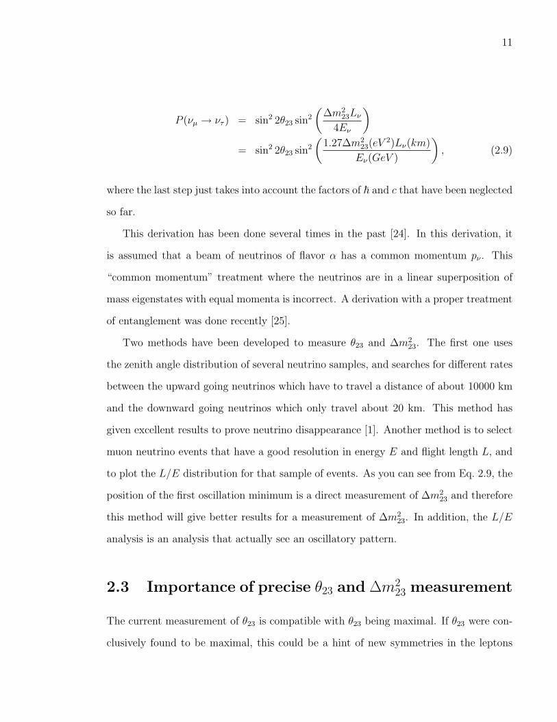
P (νµ → ντ ) = sin2 2θ23 sin2
(∆m2
23Lν4Eν
)= sin2 2θ23 sin2
(1.27∆m2
23(eV 2)Lν(km)
Eν(GeV )
), (2.9)
where the last step just takes into account the factors of ~ and c that have been neglected
so far.
This derivation has been done several times in the past [24]. In this derivation, it
is assumed that a beam of neutrinos of flavor α has a common momentum pν . This
“common momentum” treatment where the neutrinos are in a linear superposition of
mass eigenstates with equal momenta is incorrect. A derivation with a proper treatment
of entanglement was done recently [25].
Two methods have been developed to measure θ23 and ∆m223. The first one uses
the zenith angle distribution of several neutrino samples, and searches for different rates
between the upward going neutrinos which have to travel a distance of about 10000 km
and the downward going neutrinos which only travel about 20 km. This method has
given excellent results to prove neutrino disappearance [1]. Another method is to select
muon neutrino events that have a good resolution in energy E and flight length L, and
to plot the L/E distribution for that sample of events. As you can see from Eq. 2.9, the
position of the first oscillation minimum is a direct measurement of ∆m223 and therefore
this method will give better results for a measurement of ∆m223. In addition, the L/E
analysis is an analysis that actually see an oscillatory pattern.
2.3 Importance of precise θ23 and ∆m223 measurement
The current measurement of θ23 is compatible with θ23 being maximal. If θ23 were con-
clusively found to be maximal, this could be a hint of new symmetries in the leptons

12
sector such as the µ− τ interchange symmetry [26]. One prediction of the µ− τ inter-
change symmetry is that θ13 ≈ 0 and that the deviation of θ23 from maximum and of
θ13 from zero is related to the ratio of the solar mass mixing to the atmospheric mass
mixing (ε ∼√
∆m212/∆m
223).
Measuring ∆m223 to an extreme precision is not as compelling as the precision mea-
surement of θ23. Our current measurement is already good to about 10 percent, and
improving this measurement is only interesting for comparison with measurements made
by other experiments like MINOS [27]. However, as in the CKM case, over-constraining
the parameter space can be an efficient way to find hints of new physics. Finally if
the precision of the ∆m223 measurement was smaller than the value of ∆m2
12, the mass
hierarchy of neutrino could be resolved.
2.4 Remaining open questions
After the measurement of θ23 through atmospheric neutrinos and θ12 through solar and
reactor neutrinos, the remaining open questions are about θ13, the CP phase δ, and the
mass hierarchy of neutrinos. We already know that θ13 is small but it is not known yet
whether it is zero or not. The current best limit on θ13 is θ13 < 0.04 at 2σ and it is given
by the Chooz experiment [28]. The oscillation of νµ to νe is a good probe of θ13. The
next generation of neutrino experiments will use this oscillation to try to measure θ13.
The T2K experiment (Tokai to Kamioka) [29] is an electron neutrino appearance
experiment; it uses a beam of muon neutrinos starting at J-PARC (Japan Proton Accel-
erator Research Complex) in Tokai, directed at Kamioka. The Double Chooz experiment
[30] is an upgrade of the current Chooz experiment and makes use of reactor neutrinos.
If θ13 is found to be non-zero, then the search for the CP phase δ will start. One
way to measure δ is through long-baseline neutrino appearance experiments. These
kinds of experiments will be well-suited to solving the mass hierarchy. Several proposals

13
for such experiments already exist in Japan with the T2KK proposal [31], in the US
with the Fermilab to DUSEL proposal [32], and in Europe with the CERN-MEMPHYS
proposal [33].
Chapter 3
Other neutrino oscillation
experiments
In this Chapter I will very briefly review the other neutrino experiments that measure
parameters from the PMNS matrix and that have presented results as of spring 2009.
Different experiments are able to probe different sectors of the PMNS matrix. Atmo-
spheric neutrinos probe mainly the 2-3 sector (which involves ∆m223 and sin2 2θ23), solar
neutrinos mainly the 1-2 sector. The flight length of reactor neutrinos can be adjusted
to probe either the 1-2 or the 1-3 sector. And finally, the flight length and the energy of
neutrino beam can be adjusted to probe the 2-3 or the 1-3 sector. There are experiments
designed to make use of each of these configurations.
For results from LSND [34] and from MiniBooNE [35] please see their respective
references.
14

15
3.1 Solar neutrinos θ12: Homestake, Kamiokande,
IMB, SNO, Borexino
The Homestake experiment [11] is radiochemical experiment using chlorine that was
built in 1965-67 and operated until 1984. It was the first to attempt to measure the
solar neutrino flux. Their result is famous as it is the first one to notice an discrepancy
between the solar neutrino flux calculation and the solar neutrino flux measurement.
This discrepancy is often referred to as the “solar neutrino problem. Their results was
then confirmed by water Cherenkov detectors like Kamiokande [13] in Japan, IMB [14]
in the United States and finally the Super-Kamiokande solar analysis [36].
The Sudbury Neutrino Observatory (SNO) experiment confirmed Super-Kamiokande
results about solar neutrino [37]. The SNO results were a very nice confirmation of the
neutrino oscillation theory. SNO was able to study both neutral current interactions and
charged current interactions. In the case of charged current interactions, the outgoing
lepton is studied, and it is therefore possible to tell the flavor of the neutrino at the time
of the interaction. Disappearance of electron neutrinos was studied through charged
current interactions. In the case of neutral current interactions on the other hand, the
flavor of the neutrino cannot be determined as the recoiling nucleon is observed instead
of the outgoing neutrino. Therefore, when studying neutral currents, one studies the
total number of neutrinos regardless of the flavor. SNO found that the total number of
neutrinos is consistent with the expected solar flux, and thus the disappearing electron
neutrino must be oscillating into neutrinos of another flavor [37].
Finally Borexino [38] is one of the “next generation” solar neutrino experiment. It
uses liquid scintillators to study neutrino oscillation through the measurement the Be-7
line neutrino flux (E = 0.861 MeV ).

16
3.2 KamLAND (∆m212) and Chooz (θ13)
KamLAND, Chooz are two experiments which uses neutrinos from nearby nuclear re-
actors. The experiments are located at different distances from the nuclear plants, and
therefore probe different oscillation parameters. KamLAND probes the 1 − 2 sector
while Chooz probes the 1− 3 sector. These two experiments use electron anti-neutrinos
detected via inverse beta decay to do their measurement.
KamLAND is located in the Kamioka mine and uses neutrinos coming from 55 nu-
clear reactors distributed all around Japan. The latest KamLAND results are presented
in Ref. [39] and the best fit values are ∆m212 = 7.58+0.14
−0.13(stat)+0.15−0.15(sys)× 10−5 eV 2 and
tan2(θ12) = 0.56+0.10−0.07 (stat)+0.10
−0.06 (sys). Combining their results with the solar neutrino
data from SNO and Super-Kamiokande the best fit results are ∆m212 = 7.59+0.21
−0.21 ×
10−5 eV 2 and tan2(θ12) = 0.47+0.06−0.05.
Chooz is located in the north of France, and uses neutrinos coming from a reactor
located 1km away from the detector and is sensitive to the value of θ13. So far Chooz
results are consistent with θ13 = 0 [28]. An upgrade of the experiment, double-Chooz
[30] is planned. The upgrade involves a second detector located at 300 m from the
nuclear cores, and an improved detector at the site of the Chooz experiment (at 1 km
from the cores). The experiment is scheduled to start running with one detector in 2009
and with the second detector in 2010.
3.3 K2K and MINOS
All the past and current beam experiments are muon neutrino beam experiments looking
at muon neutrino disappearance. K2K is located in Japan while MINOS is an American
project. K2K finished running in 2004, while MINOS is currently taking data. There
are two future experiments (T2K and NOνA) which will be looking for electron neutrino

17
Parameter best fit 2σ 3σ∆m2
12 [10−5 eV 2] 7.65+0.23−0.20 7.25-8.11 7.05-8.34
|∆m223| [10−3 eV 2] 2.40+0.12
−0.11 2.18-2.64 2.07-2.75sin2 θ12 0.304+0.022
−0.016 0.27-0.35 0.25-0.37sin2 θ23 0.50+0.07
−0.06 0.39-0.63 0.36-0.67sin2 θ13 0.01+0.016
−0.011 ≤ 0.040 ≤ 0.056
Table 3.1: Current status of oscillation parameter measurements (Ref.[4]).
appearance in a muon neutrino beam in order to measure θ13.
K2K (KEK to Kamioka) was the first muon neutrino beam experiment and the first
to provide a measurement of θ23 which did not involve atmospheric neutrinos [40]. It
used a muon neutrino beam of about 1.3 GeV produced at KEK detected in the Super-
Kamiokande detector located 250 km away from KEK. Their best fit point for sin2 2θ23
is 1 and their best fit point for ∆m223 is 2.8× 10⁻³ eV 2 [40].
MINOS uses the Fermilab NuMI beam and detects neutrinos using two detectors: a
close detector located at 1.04 km from the NuMI target and a far detector located at
735 km. The νµ energy is around 5-10 GeV. The latest best fit results from MINOS are
|∆m223| = 2.43± 0.13× 10⁻³ eV 2 at 68% confidence level and sin2(2θ23) > 0.90 at 90%
confidence level. More details about the MINOS results can be found in [27].
3.4 Current neutrino oscillation results
The current status of the measurements of neutrino oscillation parameters is described
by T.Schwetz et al. [4]. They perform global fits to all the data currently available to
give the best measurements of the parameters in the 1-2 sector and the 2-3 sector. They
also set a limit on θ13. Their results are summarized in Table 3.1 and figures of the
global fits are presented in Fig. 3.1-3.3.

18
Figure 3.1: Determination of the leading “solar” oscillation from the interplay of datafrom artificial and natural neutrino sources. The χ2-profiles and allowed regions at 90%and 99.73% confidence level are shown for solar and KamLAND, as well as the 99.73%C.L. region for the combined analysis. The dot, star and diamond indicate the bestfit points of solar data, KamLAND and global data respectively. The fit was alwaysminimized with respect to ∆m2
31, θ23 and θ13, including always atmospheric, MINOS,K2K and Chooz data.(Ref.[4])

19
Figure 3.2: Determination of the leading “atmospheric” oscillation from the interplayof data from artificial and natural neutrino sources. The χ2-profiles and allowed regionsat 90% and 99.73% confidence level are shown for atmospheric and MINOS, as well asthe 99.73% C.L. region for the combined analysis (including also K2K). The dot, starand diamond indicate the best fit points of atmospheric data, MINOS and global datarespectively. The fit was always minimized with respect to ∆m2
21, θ13 and θ13, includingalways solar, KamLAND and Chooz data.(Ref.[4])

20
Figure 3.3: Constraints on sin2 θ13 from global data.(Ref.[4])

Chapter 4
The Super-Kamiokande Detector
The Super-Kamiokande detector is a 50 kilo-tonne water Cherenkov detector located
in a zinc mine, close to the town of Kamioka in the prefecture of Gifu, Japan. It is
part of the Kamioka neutrino observatory which is operated by the Institute for Cosmic
Ray Research (ICRR) of the University of Tokyo. It is about 1 km underground, which
corresponds to about 2700 m of water overburden. The Super-Kamiokande detector uses
Cherenkov light to detect solar and atmospheric neutrinos, and to search for nucleon
decay. There are three distinct data-taking periods (SK1, SK2 and SK3), and the
detector changed between each of them. First, I will describe the Cherenkov effect in
Section 4.1 and then I will describe the detector and the changes made to the detector
between each data-taking period in Section 4.2.
4.1 Cherenkov effect
When an electro-magnetically charged particle travels faster than the speed of light in a
given medium, a cone of Cherenkov light is emitted. The aperture of the cone θ depends
on the refractive index of the medium and the velocity of the particle: cos θ ≡ 1nβ
where
n is the refractive index of the medium and β ≡ v/c. In the case of water, where
n = 1.34 in the visible range, the Cherenkov angle is 42 for a particle traveling at
21
22
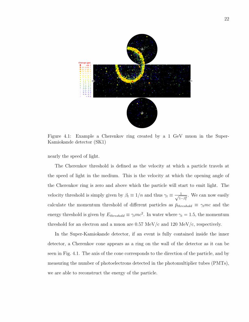
Figure 4.1: Example a Cherenkov ring created by a 1 GeV muon in the Super-Kamiokande detector (SK1)
nearly the speed of light.
The Cherenkov threshold is defined as the velocity at which a particle travels at
the speed of light in the medium. This is the velocity at which the opening angle of
the Cherenkov ring is zero and above which the particle will start to emit light. The
velocity threshold is simply given by βt ≡ 1/n and thus γt ≡ 1√1−β2
t
. We can now easily
calculate the momentum threshold of different particles as pthreshold ≡ γtmc and the
energy threshold is given by Ethreshold ≡ γtmc2. In water where γt = 1.5, the momentum
threshold for an electron and a muon are 0.57 MeV/c and 120 MeV/c, respectively.
In the Super-Kamiokande detector, if an event is fully contained inside the inner
detector, a Cherenkov cone appears as a ring on the wall of the detector as it can be
seen in Fig. 4.1. The axis of the cone corresponds to the direction of the particle, and by
measuring the number of photoelectrons detected in the photomultiplier tubes (PMTs),
we are able to reconstruct the energy of the particle.

23
Figure 4.2: Schematic view of the Super-Kamiokande detector [5].
4.2 Overview of the detector
The water tank is 42 meters high, 39 meters in diameter and made of stainless steel. The
detector is separated into an inner detector (ID) and an outer detector (OD). The inner
detector is where most of the interesting physics happens, where we can reconstruct
energy and direction with good accuracy. The outer detector is a shell of about 2.5
meters and is mainly a veto region for cosmic ray muons, but it can also be used to
reconstruct the direction of particles that have enough energy to exit the inner detector.
A general view of the detector is shown in Fig. 4.2.
The inner detector is covered with 11146 (5182) 20 inches photomultiplier tubes
(Hamamatsu R3600) for SK1 (SK2) while the OD uses 1885 8 inches photomultiplier
tubes (Hamamatsu R1408 for SK1 and R5912 for tubes added for SK2 and SK3).
Wavelength shifter plates are attached to the OD PMTs as it was done in the IMB

24
Figure 4.3: Details of the stainless steel structure, and mounting of the PMT [5].
experiment [41]. This increases their collection efficiency by about a factor of 1.5 but the
wavelength shifter plates also broaden the timing resolution of the OD PMT by about 2
ns. This is a reasonable price to pay for the gain in collection efficiency since the main
purpose of the OD is to act as a veto counter.
All the PMTs are mounted on the same stainless steel structure. The inner PMTs
are facing inwards and the outer PMTs outwards. The inner and outer detectors are
separated by two layers of polyethylene terephthalate sheets, referred to as “black sheets”
mounted on each side of the structure that holds the PMTs. The walls of the outer
detector are covered with white Tyvek sheets in order to reflect photons towards the
OD PMTs. Tyvek is a paper-like material that is very solid and reflects light in the UV
with a good efficiency. Details of the stainless steel structure, and the mounting of the
PMT is shown in Fig. 4.3.
The cables that connect the PMTs to the electronic huts located on the top of the
detector pass through 12 cable holes. Four of these twelve holes are above the ID and
would prevent Cherenkov light from being seen in the OD. In order to detect cosmic
ray muons that enter the detector through one of these cable hole, veto counters were
added in April 1997 and are presented in Fig. 4.4.

25
Figure 4.4: Veto counters placed above the cable bundles to reject cosmic ray muons.
4.2.1 History of the Super-Kamiokande detector and differ-
ences in the detector between each data-taking period
There are differences in the SK detector between the three data-taking periods completed
as of September 2008. SK1 is the original design with a 40% photo-coverage of the ID
and it is extensively described in the SK NIM paper published in 2003 [5]. After five
years of data-taking with the SK1 detector, it was decided to replace the failed OD
PMTs with newer tubes. To do so, the detector had to be switched off and emptied.
This happend in 2001 andthis is the end of the SK1 data-taking period. In November
2001, during the refilling operation that followed the upgrade, there was an accident
where half of the PMTs were destroyed by a chain reaction initiated by the implosion
of one of the bottom ID PMTs. In order to restart operation quickly after the accident,
the remaining PMTs were redistributed in the whole ID, and therefore the SK2 data-
taking period has a 20% photo-coverage. The OD could be restored to its full coverage
immediatly since less PMTs were necessary. At that time, it was also decided to add

26
Figure 4.5: 20 inch PMT in its acrylic shell. Shell was added after SK1.
an acrylic shell around each ID PMT in order to avoid another accident of the same
kind. The acrylic shells are a source of radioactive background for analyses that use
solar neutrinos. A 20 inch ID PMT with the acrylic shell is shown in Fig. 4.5.
While during the SK1 period all the OD PMTs came from the IMB experiment [42],
after the accident only 650 OD PMTs were IMB PMTs, the rest of the OD coverage was
done using a new model of Hamamatsu 8 inches PMT. Since new OD PMTs have a better
timing resolution than the IMB PMTs, there are differences in the SK software that
concerns the OD. (See Chapter 6 about Reduction and Chapter 7 about Reconstruction.)
After two and a half years of data-taking with half the ID photo-coverage, enough new
ID PMTs had been produced to recover the full photo-coverage of the inner detector,
and therefore in October 2005, SK2 ended and in July 2006, SK3 started. For SK3 it was
also decided to segment the outer detector in order to better reject cosmic ray muons
which clip the corner of the detector (“corner clipper muon” events). More details about
the OD segmentation for SK3 can be found in Appendix A. Because of the acrylic shells
the number of ID PMTs in the SK3 period is not exactly the same as in the SK1 period.
In Fig. 4.6, I present the map of old versus new OD tubes for the SK2 data-taking period
and in Table 4.1 I summarize the differences between each data-taking period.

27
Characteristics SK1 (1996-2001) SK2 (2002-2005) SK3 (2006-2008)Livetime 1489 days 803 days 550 daysPhoto-coverage 40% 20% 40%Acrylic shells no yes yesNumber of ID PMTs 11146 5182 11129Number of OD PMTs 1885 1885 1885
# of R1408 OD PMTs 1885 650 611# of R5912 OD PMTs 0 1235 1274
OD segmentation no no yes
Table 4.1: Summary of differences between the SK1, SK2 and SK3 data-taking periods
Figure 4.6: Old (red empty squares) and new (full black square) PMTs for the SK2period. The SK1 period uses only old tubes, and the SK3 period is very similar to SK2.
4.2.2 Description of the PMTs
A photomultiplier tube works by accelerating single photoelectrons created on the ca-
thodic surface of the tube towards the center of the tube. Then, this signal is amplified
through an array of dynodes such that a big enough electrical signal can be read out of
the PMT. A photomultiplier tube is characterized by its single photoelectron efficiency,
(ie, how good it is at detecting single photon), its peak quantum efficiency, its collection

28
Figure 4.7: Schematic of a 20 inch ID PMT [5].
efficiency and its gain, (ie, for a given photoelectron, how much is the signal amplified).
The characteristics of both kinds of PMTs used in the Super-Kamiokande detector can
be found in the next two subsections. More details about the PMTs can be found in
the SK NIM paper [5].
Inner PMTs
The PMTs used in the inner detector are 20 inches in diameter (Hamamatsu R3600).
The dynamic range of the ID PMTs goes from a single photoelectron (pe) to about
300 pe. The peak quantum efficiency is about 21% at 360-400nm and the collection
efficiency is 70% at the first dynode. The gain is of the order of 107 when the PMTs
are operated with a high voltage supply ranging from 1700 V to 2000 V. Finally, the
timing resolution of an ID PMT is 2.2 ns. A schematic view of the 20 inch ID PMT is
presented in Fig. 4.7.
Outer PMTs
We have two kinds of OD PMTs. When the Super-Kamiokande detector was first built,
the old IMB [42] tubes were used in the outer detector, but after the accident, most

29
Hamamatsu 8-inch PMT R1408 (IMB) R5912 (new)Peak wavelength 420 nm 420 nmSpectral response 300 nm - 650 nm 300 nm - 650 nmPeak quantum efficiency at 390 nm 25% 25%Power needed 1500V 1500 VTransit time spread (FWHM) 7.5 ns 2.4 nsGain 108 107
Number of stages 13 10Dynode structure venetian blind box and line
Table 4.2: Specifications of Hamamatsu R1408 8-inch PMT and R5912 8-inch PMT.
Figure 4.8: Schematic of a 8 inch R5912 OD PMT. (Picture taken from the Hamamatsuwebsite [43])
of the tubes had to be replaced. The IMB tubes are Hamamatsu R1408, and the new
tubes are Hamamatsu R5912. Specifications for both kinds of tubes are presented in
Table 4.2, and a schematic view of the R5912 PMT is shown in Fig. 4.8.
It was often quoted [5, 42] that the timing resolution (transit time spread) of the
R1408 PMT is 13 ns without the wavelength shifter plates. This is the timing resolution
for a single pe illumination. The value given in Table 4.2 is the value given on the
specification sheet of Hamamatsu. The quantum efficiency for both kind of tubes is

30
Figure 4.9: Quantum efficiency for R1408 8-inch tubes (left) (figure taken from [42])and R5912 8-inch tubes (right) from Hamamatsu specifications sheet [43]).
shown in Fig. 4.9. (Better plot available on spec sheet of R1408, but need to be scanned)
4.3 Overview of electronics and DAQ
In this Section, I will describe the electronics and the data acquisition (DAQ) system.
This section is highly inspired from the Super-Kamiokande NIM paper [5]. All the DAQ
electronics for the Super-Kamiokande detector are located on top of the detector in four
“electronic huts.” Each huts corresponds to one quadrant of the detector. Each PMT is
connected to its hut by a coaxial cable. The cables run on the outer side of the stainless
steel structure. The data acquisition system for the ID PMTs and for the OD PMTs
are separated.
4.3.1 ID electronics and DAQ
A schematic view of the ID data acquisition system can be found in Fig. 4.11. The PMT
cables are connected to a TKO (Tristan KEK online) module called ATM (Analog Tim-

31
Figure 4.10: A schematic view of the analog input block of the ATM. Only one channelis shown in the figure. Dashed arrows show the PMT signal, its split signals, andaccumulated TAC/QAC signals. Solid arrows show the logic signals which control theprocessing of the analog signals [5].
ing Module) and shown in Fig. 4.10. The purpose of the ATM is to convert the analog
signal of each PMT into a digitized signal containing the charge and time information.
There is one ATM for every 12 PMTs. The signal for each PMT is split into four so
that it can be used by several sub-systems. Part of the signal is used to build a variable
called HITSUM which will be used for the trigger. The trigger is described in more
details later in this chapter. If the charge deposited in one PMT is greater than 1/4 pe
then the PMT was “hit”. If a PMT was hit then the ATM generates a 15 mV pulse
with a 200 ns width, these pulses are gathered at the front of the ATM and added to
the global HITSUM. Another part of the signal is integrated in charge by a Charge-to-
Analog converter (QAC) and in time by a Time-to-Analog converter (TAC) so that if a
trigger is received the signal can be digitized and stored. There are two QAC and TAC
for each channel so that if two events occur very close to each other, they can both be
stored. The last fourth of the signal is used to build up the PMTSUM (total number of
PMT that were hit).
The high voltage supply for the ID is provided by 48 CAEN SY527 main frames.
Each of the frames supports 10 high voltage cards which can distribute power to 24

32
Figure 4.11: The ID data acquisition system [5].
channels. The high voltage supplies are monitored and can be operated remotely by a
slow control monitor.
There are 946 ATM modules distributed in the four quadrant huts. If a trigger
occurs, the trigger module generates an event number and pass this information to the
ATM module.
4.3.2 OD electronics and DAQ
The OD data acquisition system is similar to the ID system. The signal from each PMT
is digitized, then combined into a HITSUM and if the HITSUM is larger than a given
threshold or if there was on ID trigger, the information is read out. Each OD PMT is
supplied with high voltage through a coaxial cable and the same cable carries the analog
signal back to the corresponding quadrant hut. There is one high voltage mainframe in
each quadrant hut and each mainframe controls 48 channels. Each channel is connected
to a “paddle card” which distributes the power to 12 PMTs. The paddle cards were
built at BU (check). At the end of the SK1 period, the paddle cards were upgraded
such that it was easier to disable dead or noisy channels. Zener diode jumpers were also
added so that the high voltage could be fine tuned for a single PMT. Instead of ATMs,

33
the OD uses charge-to-time conversion modules called QTC in order to measure the hit
and charge of each PMT and to convert this information into a format which can be
read and stored by the Time-to-Digital converters (TDC). A more complete description
of the OD DAQ can be found in the SK NIM paper [5].
4.3.3 Trigger
There are two kinds of trigger, a hardware trigger, and a software trigger. The software
trigger called the Intelligent trigger is designed to select low energy events from solar
neutrinos. It is not used in the atmospheric neutrino analysis and therefore I will not
describe it here in detail. More information about the Intelligent trigger can be found
in the SK NIM paper [5].
There are two possible hardware triggers. One uses the ID information with three
different energy thresholds, while the other one uses the OD information. The ID
triggers use the HITSUM signal generated by the ATM module. The HITSUM signal
is equivalent to counting the number of hits in the detector. For example when the
HITSUM signal crosses -320 mV this is equivalent to having 29 hits in ID PMTs. We can
also convert the number of hit PMTs into the amount of Cherenkov photons produced
by an electron, assuming a 50% collection efficiency. For example, 29 hits in the ID
PMTs correspond to a 5.7 MeV electron.
All triggers look for coincidence of hit PMTs in a 200 ns time window. The Super Low
Energy (SLE) trigger requires a hit threshold corresponding to a 4.6 MeV electron, the
Low Energy (LE) trigger requires 29 hits in the 200 ns time window, which is equivalent
to a 5.7 MeV electron being detected. The High Energy (HE) trigger requires that the
HITSUM threshold crosses -340 mV which is equivalent to 31 hit ID PMTs. Finally,
the OD trigger requires 19 hits in the OD in the 200 ns time window. Each trigger,
including the OD trigger, will trigger the readout of the entire detector. For SK2, the
trigger threshold for LE was set to 8 MeV equivalent and the HE trigger to 10 MeV.

34
The SLE threshold was suppressed. For SK3, the threshold of the triggers were set back
to their original SK1 values.
4.4 Radon hut and water purification
For the study of solar neutrinos, it is crucial to have energy thresholds as low as possible.
The main challenges for attaining these low energy thresholds come from radioactive
sources that emit photons in the detector and poor water transparency that prevents
low energy Cherenkov photons from reaching the wall PMTs.
One of the major sources of radioactivity in the Super-Kamiokande detector is the
radon that is present in the air of the mine. In order to remove this radon, fresh air
is brought from the outside of the mine, through a pipe that runs along the Atotsu
tunnel. The radon system is located in the radon “hut”, outside the Atotsu entrance.
To improve the water transparency, the water is purified by a multi-step purification
system.
More information about the radon hut and the water purification system can be
found in the Super-Kamiokande NIM paper [5].
4.5 Calibration
There are several parameters that need to be measured or calibrated in the Super-
Kamiokande experiment: the water transparency, the light scattering, the relative gain
and timing of the PMTs, and the absolute energy scale. There are several methods for
calibrating these parameters. I will give a brief overview of these methods, but more
details can be found in the Super-Kamiokande NIM paper [5].
The water transparency is characterized by the attenuation length of light in water.
Two methods are used to measure this attenuation length. A direct measurement is

35
Figure 4.12: Linac system [5].
done using a laser ball, and an indirect measurement using cosmic rays.
The light scattering and absorption parameters are measured using a combination
of dye and N2 lasers that are fired in the detector though optical fibers during normal
data taking.
The high voltage values recommended for PMTs were adjusted at the factory such
that each PMT has equal gain. Before starting the SK1 data-taking period, those
values were recalculated using a Xenon lamp setup. Since it is not possible to retake
this measurement during data taking, the measurement was redone before the SK2 and
SK3 data-taking period, and the high voltage of each PMT was adjusted accordingly.
Measuring the relative timing of PMTs is crucial for good timing resolution and thus
for good event time reconstruction. A N2 laser is used for the timing calibration.
There are several ways of measuring the absolute energy scale. The electron LINAC
system (see Fig. 4.12) is good for a low energy direct measurement. This measurement
is cross-checked with the study of the decay of 16N . Low energy calibration is important
for solar neutrinos which have energies in the 5-20 MeV range. Electrons produced in the

36
decay of cosmic ray stopping muons are a good tool to measure the absolute energy scale
in the 20-60 MeV range. Comparing decay electrons of data and Monte Carlo simulation
(MC) allows an energy resolution of a few tens of MeV. Stopping muons are a good tool
for a wide range of energies. From 60 to 400 MeV the momentum of the muon is low
enough such that the Cherenkov angle has not yet reached its limit of 42. Therefore, we
can use the fact that the Cherenkov angle is given by cos θ ≡√p2 +m2/np where p is
the momentum, m the mass, and n the refractive index of water to measure precisely the
momentum of the muon. Comparing data and MC for stopping muons in that energy
range gives an energy resolution of about 1.5%. At higher energy, we can use the fact
that the track length of the muon is proportional to its momentum. Finally, events that
are identified as π0 are used to probe the 150-600 MeV range, by reconstructing the π0
mass peak.
In summary, the energy calibration is done through LINAC data at low energy and
the resulting resolution is better than 1%, while the energy calibration at higher energy
is done through data/Monte Carlo agreement and the resulting resolution is of the order
of 2.6%. A summary of the energy resolution for the energy range where we use data/MC
comparison to do the calibration is presented in Fig. 4.13.
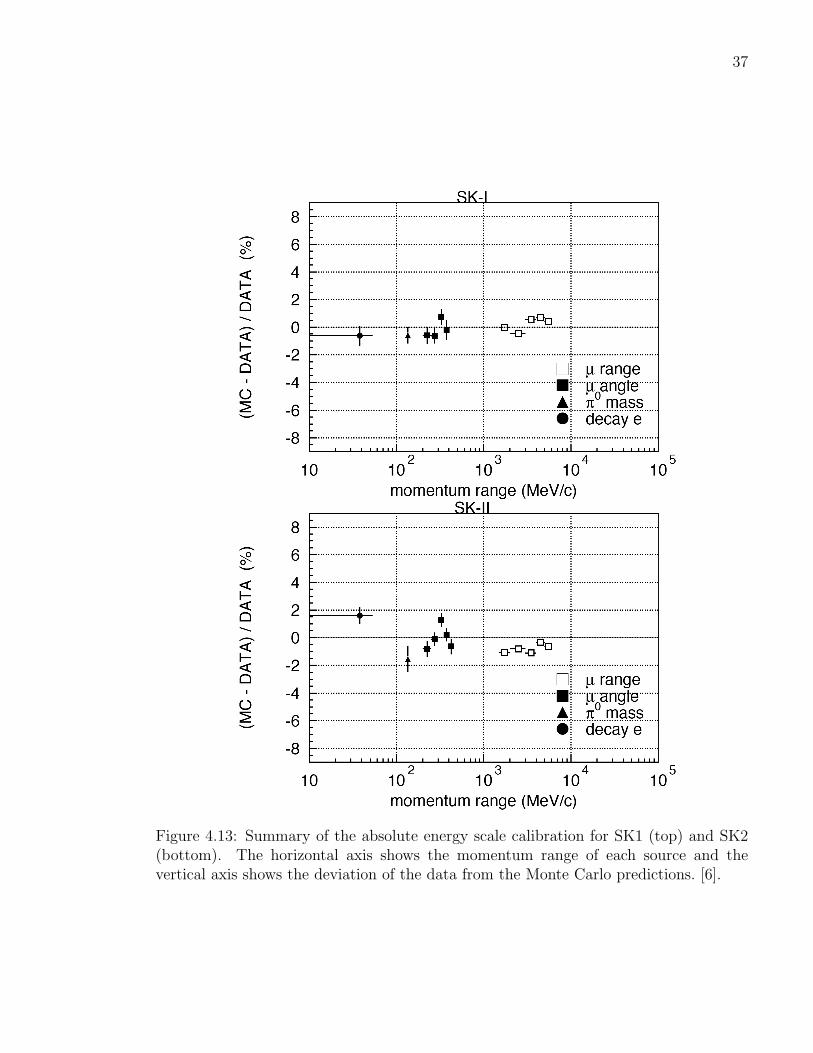
37
Figure 4.13: Summary of the absolute energy scale calibration for SK1 (top) and SK2(bottom). The horizontal axis shows the momentum range of each source and thevertical axis shows the deviation of the data from the Monte Carlo predictions. [6].

Chapter 5
Simulation
In order to tell whether the atmospheric neutrino data collected by the detector agrees
with a given model, and in order to measure the parameters of this model, we need to
compare the data against a set of Monte Carlo (MC) data. To create this set of MC
data, we first simulate the generation of atmospheric neutrinos by using the current
knowledge about the cosmic ray flux. Then we simulate the different interaction modes
that neutrinos can have with water at energies ranging from a few tens of MeV to
several GeV. After the simulation of the neutrinos themselves is completed, we still
need to simulate the detector response. Finally, the Monte Carlo sample is treated
exactly like the data, we apply reduction tools (Chapter 6) and reconstruction tools
(Chapter 7) to create the final Monte Carlo set.
5.1 Atmospheric neutrino flux
Atmospheric neutrinos are created when cosmic rays (mainly consisting of protons) hit
the atmosphere and create charged pions and kaons. Pions mainly decay to a muon
neutrino and a muon, while kaons have two main decay modes.
38

39
π+ → νµµ+ (100%)
K+ → νµµ+ (63%)
→ π+π0 (21%)
→ π+π+π− (6%)
(5.1)
The muons then decay to neutrinos:
µ+ → e+νµνe. (5.2)
The energy spectrum of atmospheric neutrinos is very wide and ranges from a few MeV
to several GeV. This is due to the large range of cosmic ray proton energies. Depending
on the energy of the cosmic ray proton, different ratios of pions to kaons are produced
and therefore different ratio of muon neutrino to electron neutrino. At low energies
where cosmic ray protons mainly produce pions, the ratio of νµ to νe is about two. It
increases at higher energies, when kaons start to be produced.
The simulation of atmospheric neutrinos for the Super-Kamiokande experiment uses
the neutrino flux calculation done by Honda et al. [44]. There are other atmospheric neu-
trino flux calculations done by G. Battistoni et al. [45] (Fluka flux) and G. Barr et al. [46]
(Bartol flux). The difference between these models is used to estimate the systematic
uncertainties on the neutrino flux. The calculated energy spectrum of atmospheric neu-
trinos at the Super-Kamiokande site for the Honda flux, Fluka flux and Bartol flux is
shown in the left panel of Fig. 5.1. The right panel shows the flavor ratio of νe + νe to
νµ + νµ.
The primary cosmic ray flux depends on the solar activity. If the solar activity is

40
Figure 5.1: Predictions of the direction averaged atmospheric neutrino flux (left) andthe flavor ratio (right) [6].
high (solar maximum), the solar winds are strong and the flux of cosmic rays that reach
the atmosphere is decreased. Similarly if the solar activity is low (solar minimum), the
cosmic ray flux is increased. For 1 GeV cosmic rays, the flux at solar minimum differs by
a factor of two from the flux at solar maximum. For 10 GeV cosmic rays the difference
is about 10% while 100 GeV cosmic rays are not affected. Another effect taken into
consideration is the geomagnetic field, which acts as a shield for low momentum cosmic
rays.
After the primary cosmic rays hit the atmosphere, secondary particles (mainly pi-
ons, kaons and muons) are created as described in Eq. 5.1. The decay of secondary
mesons creates mainly muons and neutrinos. In the calculation of the neutrino flux, the
interactions and the propagation of particles is done in a 3-dimensional manner. This
is especially important for the L/E analysis because the two main effects of applying a
3-D treatment versus a 1-D treatment are:
1. An enhancement of the neutrino flux for near-horizontal directions.
2. Lower production heights of neutrinos in the atmosphere. This also affects mainly
near-horizontal neutrinos.

41
Figure 5.2: Example of 1D versus 3D flux calculation. The solid arrows denote theprimary cosmic ray, while the dotted arrows denote the neutrinos.
The first effect is due to a difference in effective area for primary cosmic rays that
generate horizontally incoming neutrinos as it can been seen in Fig. 5.2. This effect is
especially important for low energy neutrinos (1 < GeV). In that case, the incoming
cosmic ray and the outgoing neutrinos are less likely to be colinear, either because of
the kinematics of hadronic interactions, or because the outgoing muon can more easily
be bent by the geomagnetic field if it has low momentum.
The second effect is explained by the fact that horizontal cosmic rays have to travel
a larger distance to reach the same altitude as vertical cosmic rays. Therefore horizontal
cosmic rays produce neutrinos higher in the atmosphere than vertical cosmic rays. In
the 1D treatment only horizontal cosmic rays can produce horizontal neutrinos in the
detector, but in the 3D treatment this is not the case. As a result, the production
height of horizontal neutrinos is lowered. The 50% accumulation probability is the
height above which 50% of the neutrinos of a given energy have been produced. We
can see in Fig. 5.3 that applying a 3-D treatment does decrease the production height
of horizontally incoming neutrinos, especially at at energies below 1 GeV.

42
Figure 5.3: 50% accumulation probability lines of neutrino production height for (a)near-vertical (cos θ > 0.95) and (b) near-horizontal (| cos θ| < 0.05) directions. Thickand thin solid lines are for νµ and νe calculated with the 3D treatment, while thick andthin dashed lines are for νµ and νe calculated with the 1D treatment [47].
5.2 Neutrino interaction
The simulation model is based on the NEUT library [48–50]. The NEUT library
was first developed to simulate the background caused by neutrino interactions in the
Kamiokande nucleon decay measurement, and it was later expanded for the study of
all atmospheric neutrinos. It is designed to simulate neutrino interactions with water
(proton and oxygen) for energies ranging from a few MeV to 1 TeV. In the NEUT code,
the following interactions are considered:

43
CC/NC (quasi)-elastic scattering : ν +N → l +N ′
CC/NC single meson production : ν +N → l +N ′ +meson
CC/NC deep inelastic interaction : ν +N → l +N ′ + hadrons
CC/NC coherent pion production : ν +16 O → l +16 O + π
(5.3)
where N and N ′ are protons or neutrons and l is a lepton. The cross-section of
neutrino-electron interaction being a factor of a thousand smaller than the neutrino-
nucleon interaction at ≈ 1 GeV it is not simulated here. Each mode is described briefly
in the following subsections. These descriptions can be found in more details in G.
Mitsuka’s thesis [6].
5.2.1 Elastic and quasi-elastic scattering
The scattering of neutrinos off a free proton has been described by Llewellyn-Smith in
Ref. [51]. For the scattering off bound nucleus of 16O, nuclear effects like the Fermi
motion, or the Pauli exclusion principle are dealt with following the work of Smith and
Moniz [52].
In general, neutrino scattering off nucleon involves form factors [53]. Form factors
are a way to describe the effect of the nucleon not being a pointlike particle. Form
factors are usually labelled F (q2), where q2 is the square of momentum transfer. The
differential cross-section is therefore modified as follows:
dσ
dΩ=dσ
dΩpointlike× F (q2) . (5.4)
Empirically, it is found that the form factors can be fitted by the dipole formula:

44
Figure 5.4: Quasi-elastic cross-sections for (a) νµ and (b) νµ computed with the NEUTlibrary and with experimental data. The solid and dashed curves indicate the scatteringof free and bound nucleon respectively [6].
F (q2) ≈ 1
(1 + q2/M2)2, (5.5)
where M is just a parameter determined by fitting to experimental data. In the case
of neutrinos scattering, there are two form factors, one for vector couplings, specified
by the vector mass MV and one for axial vector couplings, specified by the axial vector
mass MA.
For reference, I give here the values of some parameters used in the simulation. The
vector mass MV is set to 0.84 GeV, and the axial vector mass MA is set to 1.21 GeV
according to experimental results [35, 54, 55]. The value of MA is consistent with the
value used by other experiments like K2K and MiniBooNE. The uncertainty on MA is
estimated to be 10%. The axial vector coupling constant gA is measured in polarized
nucleon beta-decay [56] and is set to 1.232. The Fermi surface momentum is set at
225 MeV/c. The cross-sections of quasi-elastic scattering for experimental data and
calculation with the NEUT library are shown in Fig. 5.4. The solid and dashed curves
indicate the scattering of free and bound nucleons respectively.

45
5.2.2 Single meson production
Meson production occurs through baryon resonances as shown in Eq. 5.6. We use the
Rein and Sehgal model [57] to treat meson production. The model was first developed
for single pion production but it was then modified to account for single η and kaon
production. The value of MA used for meson production is also set to 1.21 GeV. Single
pions charged current cross-sections for muon neutrino a muon anti-neutrino are shown
in Fig. 5.5 and Fig. 5.6.
ν +N → l +N∗
N∗ → N ′ +meson
(5.6)
5.2.3 Deep inelastic scattering
When deep inelastic scattering occurs, several hadrons can be created, and we call these
outgoing hadrons the hadronic system. We treat the case of single pion production
separately as seen in the previous section. For reference, here are several parameters
used to compute deep inelastic cross-sections. The GRV98 [58] parton distribution
function is used, and the corrections from A. Bodek and U.K. Yang are applied [59].
The kinematics of the hadronic system is calculated with a different method depending
on the invariant mass. For 1.3 GeV/c2 < W < 2.0 GeV/c2, only outgoing pions are
considered and for W > 2.0 GeV/c2 we use the PYTHIA/JETSET [60] package to
simulate all sorts of outgoing mesons (not only π but also K, η, ρ, etc).

46
Figure 5.5: Single π charged current cross-sections (νµ). Solid curves are the NEUTcalculations, experimental data are overlaid and described in panel (d) [6].
5.2.4 Coherent pion production
Coherent pion production is a neutrino interaction with an oxygen nucleus, where the
nucleus remains the same and a pion with the same charge as the incoming weak current
is produced. Here again we use the formalism developed by Rein and Sehgal [61].
The measurements by the K2K-SciBar detector set an upper limit on the cross-
section of charged current coherent pion production [62]. Since this upper limit is sig-
nificantly lower than the predicted cross section, some modifications to the calculation
were made by Rein and Seghal [63] and implemented in the simulation. The modifica-
tions account for the non-vanishing lepton mass in charged current interactions. This
suppresses the cross section by about 25% at 1.3 GeV due to interference of the axial

47
Figure 5.6: Single π charged current cross-sections (νµ). Solid curves are the NEUTcalculations, experimental data are overlaid and described in panel (d) [6].
vector and the pseudo-scalar (pion-exchange) amplitudes. The cross sections for charged
current and neutral current are shown in Fig. 5.8.
5.2.5 Nuclear effects
Secondary interactions of mesons which are produced in neutrino interactions with nu-
cleons inside the 16O nuclei also need to be simulated. In particular the interactions of
pions are very important since the pion-nucleon cross-section is quite large for neutrino
energies above 1 GeV. The pion interactions in the 16O nuclei that have been considered
are: inelastic scattering, charge exchange and absorption.

48
Figure 5.7: Deep inelastic cross-sections for charged current νµ and νµ interactions. Up-per (lower) curves are for νµ (νµ). NEUT calculations are shown for two different partondistribution calculation and with or without Bodek-Yang corrections. Experimental dataare overlaid [6].
Figure 5.8: The cross sections for coherent pion production off the carbon nucleusfor charged current interaction (left) and neutral current (right) by two models withexperimental data. The solid, dashed and dotted curves stand for Rein and Sehgal withlepton mass effects, Rein and Sehgal without lepton mass effects, and Kartavtsev et al.respectively. On the left figure, the arrow indicates the experimental upper limit byK2K [62] and on the right experimental data are from CHARM, MiniBooNE, Aachen-Padova and Garmaelle [6].

49
5.3 Detector simulation
All the particles that are produced in the NEUT simulation are then processed with the
detector simulation code. The detector simulation tracks the particle through water,
generates Cherenkov light, propagates the light through the water, and finally simulates
the PMT and the electronics response. The detector simulation is written with the
GEANT3 package [64]. To simulate the hadronic interactions in water we use the
CALOR package [65]. The complete list of processes which are simulated is given in
Table 5.1. In order to estimate the systematic uncertainty on the hadron simulation,
we compare the results of our detector simulation with the CALOR package, and the
Fluka model. For the light propagation in water we consider Rayleigh scattering, Mie
scattering, and absorption.
γ (e+,e−) pair productionCompton scatteringPhotoelectric effect
e± Multiple scatteringIonization and δ-rays productionBrehmsstrahlungAnnihilation of positronGeneration of Cherenkov radiation
µ± Decay in flightMultiple scatteringIonization and δ-rays productionDirect (e+,e−) pair productionNuclear interactionGeneration of Cherenkov radiation
Hadrons Decay in flightMultiple scatteringIonization and δ-rays productionHadronic interactionsGeneration of Cherenkov radiation
Table 5.1: List of processes considered in the GEANT simulation.

Chapter 6
Data Reduction
The goal of data reduction is to select neutrino events out of the dataset selected by the
trigger. The raw data is processed in real time by the first stage of reduction. The rest
of the data reduction happens later. Before reduction, about 106 events are collected
every day. Most of these are cosmic ray muons. Data reduction can be split into three
categories. FC (fully-contained) reduction selects neutrino events for which none of the
visible outgoing particles exit the inner detector and therefore have only a few hits in the
outer detector for. PC (partially-contained) reduction selects neutrino events in which
the outgoing lepton exits the inner detector and deposits a lot of energy in the outer
detector. Finally UPMU (upward-going muon) reduction selects muon events going
upwards. Upward-going muons are the result of neutrino interactions in the rock below
the detector. A schematic view of each event sample can be found in Fig. 6.1. The FC
and PC samples have the same livetime, while the UPMU sample, which is less sensitive
to detector effects has a larger livetime. Since the UPMU sample is not used in the L/E
analysis, it will not be described further.
The separation between FC and PC events is based on the number of hits recorded
in the outer detector. The systematic error on this separation is 0.6% for SK1 and 0.5%
for SK2.
I personally worked on improving PC reduction for the SK3 data-taking period, so in
50

51
Figure 6.1: Schematic view of different event samples.
addition to presenting a brief overview of FC and PC reduction for SK1 and SK2 here,
I will present the details of the PC reduction improvements for SK3 in Appendix A.
6.1 Fully-contained reduction
First I present an overview of the FC reduction results and then I describe the five levels
of FC reduction in the following subsections.
6.1.1 First reduction
The goal of the first reduction is to remove low energy background due to radioactive
decay and to remove cosmic ray muons. The cuts applied in the first reduction must
be very stable and quite loose since the first reduction is run online. The goal is to
not go back to the raw data but rather go back to the output of the first reduction if a
reduction algorithm is improved.
• PE300: The number of photoelectrons in the ID within a 300 ns sliding time window
needs to be greater than 200 for SK1 and 100 for SK2. PE300 ≥ 200(100).
• NHITA800: This is the number of hits in the outer detector in a fixed time window

52
that runs from 400 ns before the ID trigger to 400 ns after. NHITA800 ≤ 50 or the
OD trigger must be off.
• TDIFF: This is the time interval between that last event and this one. We require
that TDIFF ≥ 100µs so that we can reject electrons created by the decay of stopping
muons.
After these cuts the event rate is about 3000 events per day for SK1 and 2200 events
per day for SK2.
6.1.2 Second reduction
Second reduction has the same purpose as first reduction and is based on the same cuts
but with tighter values, but it is run offline as are all reduction stages following FC2.
• PEmax/PE300 < 0.5: With PEmax being the maximum number of photoelectrons
seen in one PMT and PE300 being the same as in the first reduction. The goal of
this cut is to remove flasher events (flasher events are described in Section 6.1.3.)
• NHITA800: NHITA800 ≤ 25 if PEtot < 100000 (50000) p.e. for SK1 (SK2), or the
OD trigger must be off.
After the second reduction step, the event rate is about 200 events per day for SK1
and 280 events per day for SK2.
6.1.3 Third reduction
Third reduction is still aimed at rejecting the remaining cosmic ray events and noise
events, but now more elaborate (and time-consuming) tools are applied.

53
Through-going muon cut
Since through-going muon are cosmic ray muons deposit a lot of charge in the inner
detector and leave an entrance and an exit charge cluster in the outer detector. We
apply the following set of cuts, which uses a special muon fitter.
• PEmax > 250 p.e.: If one of the ID PMT receive more than 250 p.e.s then the
following cuts are applied. In the SK2 case, we also ask that the total number of
hit in the ID be greater then 1000.
• mugood > 0.75: The goodness of the muon fit must be better than 0.75
• NHITAin ≥ 10 or NHITAout ≥ 10: The number of hit PMTs in the OD within 8
meters of the entrance (in) or exit (out) point must be greater than 10 in a 800 ns
time window.
Stopping muon cut
To remove stopping muons, we also use the muon fitter used for the though-going muon
cut.
• mugood > 0.5 and NHITAin ≥ 5 OR NHITAin ≥ 10: where the definitions of mugood
and NHITAin are the same as for the through-going muon cut.
Cable hole muon cut
We need to remove cosmic ray muons that enter through the cable holes described in
the detector section 4.2. We remove events that have the following characteristics:
• One hit in the veto counter.
• lveto < 4m : The vertex must be within 4 meters of the cable hole.

54
Flasher events
Flasher events are due to mis-behaving PMTs. The timing distribution of such events
is usually wider than the timing distribution of neutrino events. Events satisfying the
following criteria are considered flasher events and removed from the neutrino sample.
• For SK1: NMIN100 ≥ 14 or NMIN100 ≥ 10 if the number of hit ID PMT is less than
800. NMIN100 is the minimum number of ID hits in a 100 ns time window.
• For SK2: NMIN100 ≥ 20
Accidental muon cut
Sometimes, a cosmic ray event happens just after a low energy event. If the two events
are in the same trigger gate, the event is hard to reject because there will be no OD
activity during the trigger gate, but enough photoelectrons (coming from the muon) in
the ID to keep the event. To reject such events, we apply the following two cuts:
• NHITAOFF > 20: The number of hit OD PMTs in the fixed 500 ns time window
from 400 ns to 900 ns after the trigger is greater than 20.
• PEoff > 5000 (2500) p.e.: The number of photoelectrons in the ID in the 500 ns
time window is greater than 5000 (2500) for SK1 (SK2).
Low energy muon cut
Low energy events from electronic noise and radioactive decay are removed at this stage
by applying the following cut:
• NHIT50 < 50 (25): The number of ID hits within a 50 ns sliding time window is
less than 50 for SK1, 25 for SK2. To decide whether a hit PMT is in the 50 ns
time window, we take into account the time of flight of the photons assuming they
55
all come from the same vertex. In this case the vertex is defined as the position at
which the residual time distribution peaks. NHIT50 = 50 corresponds to a 9 MeV
event.
After the third reduction step, the event rate is about 45 events per day for SK1 and
21 events per day for SK2.
6.1.4 Fourth reduction
The goal of the fourth reduction step is to remove the remaining flasher events. Flasher
events occurs when light is emitted from the discharge of the PMT dynodes. It usually
takes time before such bad PMTs are identified and turned off, so we have to remove
flasher events in the reduction process. The characteristic of flashers is that the light
pattern emitted by these events repeats over a long period of time. By looking for such
repetition we are able to remove these events. More details about how this search is
performed was described previously [66].
The event rate after the fourth reduction is about 18 events per day for both SK1
and SK2.
6.1.5 Fifth reduction
The fifth (and last) reduction is a set of very specific cuts designed to remove the
remaining non neutrino events.
Stopping muon cut
This cut is similar to the cut applied in the third reduction, but the entrance point is
now computed by extrapolating backward the fitted track of the event instead of using
the earliest hit PMT. The cut is now:
• NHITAIN ≥ 5 where NHITAIN is defined as before.

56
Invisible muon cut
When a cosmic ray muon is below the Cherenkov threshold it is not seen in the detector
but its decay electron can be seen. Such events are called invisible muons and are
removed with the following set of cuts:
• PEtot < 1000 (500): The total number of photoelectrons in the ID is less than 1000
for SK1 and 500 for SK2.
• NHITAmaxearly > 4: The maximum number of hit OD PMTs in a 200 ns time window
going from 8900 ns to 100 ns before the trigger is greater than 4.
• NHITAmaxearly+NHITA500 > 9 if lcluster < 500cm or NHITAearly > 9 otherwise. NHITA500
is the number of hit OD PMTs in a 500 ns time window from -100 ns to 400 ns.
lcluster is the distance between two OD clusters used during the calculation of
NHITAearly and NHITA500.
Coincidence muon cut
The remaining accidental events are removed using the following two cuts:
• PE500 < 300 (150)p.e.s: The total number of photoelectrons within a 500 ns time
window going from -100 ns to 400 ns is less than 300 for SK1 and 150 for SK2.
• NHITAmaxlate > 20: The number of hit OD PMTs in a 200 ns sliding window going
from 400 ns to 1600 ns after the trigger is greater than 20.
Long tail flasher cut
This a tighter version of the cut applied in the third reduction. Events are removed if
they satisfy the following condition:

57
• For SK1: NMIN100 > 5 if the goodness of point fit is < 0.4: The minimum number
of hit ID PMTs in a 100 ns sliding time window from 300 ns to 800 ns after the
trigger is greater than 5.
• For SK2, the SK1 cut is applied and in addition we ask that the goodness of point
fit be < 0.3 and that NHITMIN100 < 6.
The event rates at the end of the fifth reduction step are about 16 events per day for
both SK1 and SK2.
6.1.6 Final FC cuts
The last cuts to be applied to select the fully-contained sample are the following:
• FV cut: the fiducial volume cut where we require an event to have a reconstructed
vertex located at more than 2 meters from the wall of the inner detector. For the
L/E analysis, we relax the fiducial volume cut a little bit. In that case, the vertex
must be 1.5 meters away from the endcaps (top and bottom) and 1 meter away
from the wall.
• NHITAC: We require that the number of hits in the outer detector be less than 10
for SK1 and 16 for SK2. This is the separation between FC and PC events.
• Evis: The visible energy must be greater than 30 MeV. The visible energy is
defined as the energy of an electro-magnetic shower that produced a given amount
of Cherenkov light.
These final cuts are not applied for every analysis, in the case of the L/E analysis
for example, the fiducial volume is extended as seen in the next Chapter. At the end
of the reduction process the event rate of the FC sample is 8.18± 0.07 and 8.26± 0.10
events per day for SK1 and SK2 respectively.
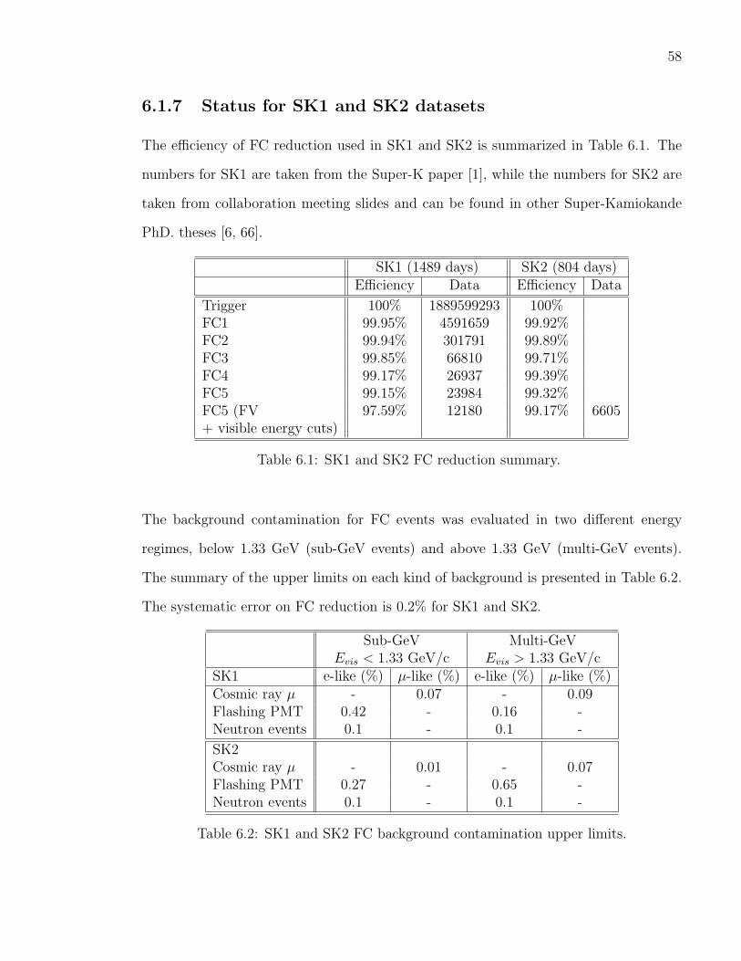
58
6.1.7 Status for SK1 and SK2 datasets
The efficiency of FC reduction used in SK1 and SK2 is summarized in Table 6.1. The
numbers for SK1 are taken from the Super-K paper [1], while the numbers for SK2 are
taken from collaboration meeting slides and can be found in other Super-Kamiokande
PhD. theses [6, 66].
SK1 (1489 days) SK2 (804 days)Efficiency Data Efficiency Data
Trigger 100% 1889599293 100%FC1 99.95% 4591659 99.92%FC2 99.94% 301791 99.89%FC3 99.85% 66810 99.71%FC4 99.17% 26937 99.39%FC5 99.15% 23984 99.32%FC5 (FV 97.59% 12180 99.17% 6605+ visible energy cuts)
Table 6.1: SK1 and SK2 FC reduction summary.
The background contamination for FC events was evaluated in two different energy
regimes, below 1.33 GeV (sub-GeV events) and above 1.33 GeV (multi-GeV events).
The summary of the upper limits on each kind of background is presented in Table 6.2.
The systematic error on FC reduction is 0.2% for SK1 and SK2.
Sub-GeV Multi-GeVEvis < 1.33 GeV/c Evis > 1.33 GeV/c
SK1 e-like (%) µ-like (%) e-like (%) µ-like (%)Cosmic ray µ - 0.07 - 0.09Flashing PMT 0.42 - 0.16 -Neutron events 0.1 - 0.1 -
SK2Cosmic ray µ - 0.01 - 0.07Flashing PMT 0.27 - 0.65 -Neutron events 0.1 - 0.1 -
Table 6.2: SK1 and SK2 FC background contamination upper limits.

59
6.2 Partially-contained reduction
The goal of most of the PC reduction process is to remove cosmic ray muons. There are
two kinds of cosmic ray muons: through-going muon events which enter and exit the
inner detector and deposit two charge clusters in the OD, and stopping muon events
which deposit an entrance charge cluster in the OD and stop in the ID. There are five
levels of PC reduction and the first reduction is run online.
6.2.1 First reduction
The cuts used in PC1 must be very simple and very stable since the first reduction is
run online.
• PEtot: The total number of photoelectrons observed in the ID must be greater
than 1000 (500 for SK2).
• TWIDA: The width of the timing distributions of OD PMTs must be smaller than
260 ns for SK1 (170 ns for SK2).
• NCLSTA: The number of hit clusters in the OD must be equal or greater than 1.
(Cut applied only for SK1)
6.2.2 Second reduction
PC2 uses very simple cuts, looking at variables like the number of hits in the OD or the
charge to remove cosmic ray muons. This reduces the number of events for which we
have to run time-consuming fitters.
• Numendcap vs numwall: (SK2) We look at the number of hits in the endcaps of
the detector and compare it to the number of hits in the wall. If the number
of hits in the endcap is smaller than the maxendcap(numwall) then the event is

60
Figure 6.2: Number of hits in the OD endcaps versus number of hits in the OD wall.Events that are above the red line (maxendcap) are corner clippers events and are rejectedduring PC reduction.
kept. This cut is designed to remove cosmic ray muons that clip the corner of the
detector (corner clipper events).
• Nouter2: Number of hits in the second highest charge OD cluster. An event
passes this cut if nouter2 ≤ 10. This cut is used to remove through-going cosmic
ray muons.
• Nouter: Number of hits in the highest charge OD cluster. An event passes this
cut if nouter ≤ 6. This is to remove both kind of cosmic ray muons. If events
have more than 6 hits then they are part of a conditional cut with PE200 (next
cut).
• PE200: Number of photoelectrons within 200 cm of the highest charged PMT in
the ID hit cluster closest to the OD hit cluster. This cut is combined with the

61
nouter cut such that an event passes the cut if (nouter < (12+ pe200 /2.0 ∗
(80.− 12.)/800.)). This cut is used to remove stopping events.
In order to pass PC2 an event has to satisfy the following criteria:
((numendcap vs numwall).and.(nouter2).and.(nouter.or.pe200)
6.2.3 Third reduction
• Flashtest: Results of the function flasher test. This cut is used to removed
flasher events due to electronic noise.
• Ehit8m: This is the number of hit OD PMTs located within 8m of the entrance
point in a fixed 500 ns time window. The entrance point is extrapolated using the
pfit direction. We require ehit8m ≤ 10 to pass the cut. This cut removes both
stopping and through-going muon events.
We ask an event to pass both cuts in order to be kept.
6.2.4 Fourth reduction
PC4 mainly uses the muon fitter mfmufit and the point fitter pfit.
• Qismsk: Total charge in the inner detector. This is to remove events with too
little energy in the ID. The cut is set at 1000 in PC4 and then at 3000 in PC5.
• Mu distance: This is the track length given by mfmufit. Long track lengths
are associated with cosmic ray muons. An event passes the cut if Mu distance
< 3000.
• Mu good: This is the goodness of the mfmufit. The goodness of fit is good only
for true muons, therefore we keep events with a bad goodness of fit. An event
passes the cut if Mu good < 0.85.
62
• Dcorn: This is the distance between the vertex found by pfit and the corner of
the tank. An event passes the cut if dcorn > 150. This removes events that are
outside the fiducial volume anyway, but it is convenient to remove these events at
this stage, as they would slow down PC5.
• Dot product: This is the dot product between the pfit direction (~dpfit) and the
vector linking the pfit vertex and the earliest saturated ID PMT (~dpmt ). An
event passes the cut if dot product = ~dpfit · ~dpmt > −0.85. This cut eliminates
cosmic ray muons that are likely to have ~dpfit and ~dpmt in the opposite direction.
An event is kept if:
(qismsk).and.(dcorn).and.(dot product).and.((mu good) .or.(mu distance))
6.2.5 Fifth reduction
PC5 is split into two distinct parts. Fast cuts that do not use any precise fitter, and
slow cuts that use several fitters like apfit, MS-fit (msfit) and others. These fitters
are described in more detail in the next chapter.
Fast cuts
First there are two very basic cuts to select partially-contained events.
• Nhitac: This is the number of hits in the OD. We use this cut to decide whether
an event is fully-contained (nhitac< 16) or partially-contained (nhitac≥ 16).
• Qismsk: This is the total charge in the ID. We keep events which have qismsk>
3000.
Then there are a set of very simple cuts, using only OD information, and designed to
remove through-going muon events.

63
• Nodcluster3: This is the number of hits in the third highest charged OD cluster.
If nodcluster3< 2 then an event passes this cut.
• Distod12: This is the distance between the first and second highest charge OD
clusters. If distod12≤ 2000 then an event passes this cut. A very large distance
would be an indication of a through-going muon.
• Odclustq2: This is the amount of charge in the second highest charge OD cluster.
If odclustq2< 10 then an event passes this cut.
If an event passes at least one of these three cuts, it is kept.
Finally we use two cuts to remove events coming from calibration runs (calsel cut), or
from runs where there was a problem with some of the electronics huts (deadsel cut).
Only events that pass the fast cuts are passed on to the slow cuts.
Slow cuts
There are several kinds of slow cuts. Cuts designed to remove junk events, stopping
muons, through-going muons, corner clippers and low energy events.
Junk cut:
• ‘‘Bye Bye’’ cut: This cut is designed to remove events that were spread across
two triggers.
• NO ID: This cut removes events where the ID data is missing.
• Ano OD: This cut removes events where the OD malfunctioned.
Muon cuts: There is one cable hole muon cut, four stopping muon cuts and three
through-going muon cuts.
Cable hole muon:

64
There are veto scintillation counters placed over the four cable holes on top of the
detector (see Chapter 4). The cut criteria to remove a cable hole muon are the following:
• Veto: One veto counter hit.
• ~dring · ~dveto−vertex > −0.8, where ~dring is the reconstructed ring direction, and
~dveto−vertex is the direction from the hit veto counter to the reconstructed vertex.
Stopping muons:
The stopping muons cuts rely on finding a cluster of OD hits close to an entry cluster
in the ID.
• Stop mu: Number of entry hits based on the msfit fitter results. If more than 10
entry hits are found, then the event fails this cut.
• Cone: This cut uses the charge information in the opposite direction of the stmfit
direction. First, we check that the stmfit goodness is greater than zero. Then
we define a cone of 8 m radius, in the backward direction found by the pfdofit
fitter. We also check that 60% of the ID charge is in the cone. If there are more
than 6 hits in this cone, then the event is rejected.
• Hits: This cut is the same as the ehit8m cut in PC3, but instead of using pfit,
we now use the precise fitter apfit. If more than 10 hits are found close to the
entry point, the event fails the cut.
• Angle: This cut uses the angle between a fitted direction and a vector linking a
fitted vertex and the center of the highest charge OD cluster. Two fitters are used,
the standard precise fitter apfit and msfit. If any of the angles are above 90
then the event is rejected.
Through-going muons:

65
The through-going muon cuts rely on finding two clusters in the OD, an entry cluster
and an exit cluster.
• Geji: This cut is used to remove “Geji” events. Those are cosmic ray muons that
are traveling vertically downwards in the volume between the ID and the OD.
They leave a “millipede-type” track in the ID which explains their name. (i.e.
millipede = geji in Japanese)
• Cluster: Using an algorithm called grad cluster, we look at the number of hits
in the first and in the second OD cluster. We ask the number of hits in the first
cluster to be less than 10 and the number of hits in the second OD cluster to be
less than 10.
• Through mu: This cut uses the number of entry and exit hits based on msfit
results. If there are more than 4 entry hits and more than 4 exit hits and if the
variable thtoflen is between 0.75 and 1.5 then the event is rejected. The variable
thtoflen is the time difference between average hit time in the top and bottom
OD clusters divided by the distance between the entry and exit points.
Corner Clipper:
• New evis: This cut is used to reject mis-reconstructed corner clipper muons using
the relation between the visible energy given by apfit and the track length from
the apfit vertex to the OD exit position.
Low Evis:
• Evis: This cut is used to remove events that have a visible energy less than
350 MeV and are inside the fiducial volume.
An event has to pass all the PC5 cuts to be accepted in the final PC sample.

66
6.2.6 Status for SK1 and SK2 datasets
The efficiency of PC reduction used in SK1 and SK2 is summarized in Table 6.3. The
numbers for SK1 are taken from the Super-K combined paper [1]. The SK2 numbers
are from collaboration meeting slides.
SK1 (1489 days) SK2 (804 days)Efficiency Data Efficiency Data
PC1 99.0% 1889599293 98.7%PC2 94.2% 34536269 94.3%PC3 93.1% 5257443 93.1%PC4 87.9% 380053 85.8%PC5 84.4% 1483 84.3% 678PC5(FV) 79.7% 911 79.4% 427
Table 6.3: SK1 and SK2 PC reduction summary.
The background contamination in the PC sample comes mainly from cosmic ray muons.
The background estimation is simply done by scanning the final data sample and count-
ing how many non-neutrino events are found inside the fiducial volume. For SK1 the
background contamination was 0.2% and for SK2 it was 0.7%.
The PC systematic uncertainties for PC1 to PC4 were estimated using two methods.
For ID cuts, the uncertainty of each cut was estimated by comparing data and MC. For
OD cuts, the uncertainty was estimated by creating several sets of Monte Carlo with
slightly different OD tuning parameters and studying how these changes affected the
PC efficiency. The uncertainty of the last step of PC reduction was again estimated by
comparing distributions of cut variables between data and Monte Carlo. All the uncer-
tainties were then added in quadrature. A more detailed description of the uncertainty
calculation is done in Ref. [67]. The final PC uncertainty for SK1 is 2.4% and for SK2 is
4.8%. The final event rate at the end of PC reduction is 0.61± 0.02 (0.53± 0.03) events
per day for SK1 (SK2).

Chapter 7
Data Reconstruction
Events that pass all the reduction steps are then reconstructed in order to be used in
analyses. The energy, the number of rings, the type of rings (electron or muon), and the
vertex of the interaction are some of the variables that are computed during the recon-
struction. In this Section, I will describe how the main variables that characterize an
event are computed. For comparison of data versus Monte Carlo of standard variables,
see Appendix B. The name of the algorithms are written for reference, and the master
routine that runs the entire reconstruction is called apfit.
7.1 Vertex fitting (tfafit)
The vertex is the first variable to be reconstructed. To do so, we apply a “3 steps”
fit. This is the first attempt at fitting the vertex and it will be improved later in the
reconstruction process.
7.1.1 Point fit (pfit)
First we look for a rough vertex position, assuming that all the light comes from a single
point source using the timing information of all PMT’s. We defined the goodness of the
point-fit vertex GP as in the following equation:
67

68
GP =1
N
∑i
exp
(− (ti − t0)2
2(1.5 · σ)2
), (7.1)
where N is the number of hit PMT’s, ti is the residual time of the ith (ie. the difference
between the hit time of the PMT t0i and the time of light of the photon between the
PMT and the vertex candidate), t0 is a free parameter representing the time of the
interaction, σ is the timing resolution (2.5 ns) and the 1.5 factor is there to improve the
performance of the fit.
Depending on the position of the vertex, the time of flight of each photon is different,
and the algorithm looks for the position which maximizes GP .
Once the point-fit fitter finds a vertex, a rough direction is also calculated using:
~d0 =∑i
qi ×~Pi − ~O0
|~Pi − ~O0|, (7.2)
where ~O0 is the vertex position found by point-fit, ~Pi is the position of the ith PMT and
qi is the detected charge in the ith PMT.
7.1.2 Ring edge search
Then we look for the edge of the main ring, and we compute a more precise direction.
The ring edge is found by looking at the distribution of observed photo-electrons as a
function of the angle of each PMT and the direction given by point-fit. The direction
is then varied around the point-fit direction in order to maximize the estimator defined
as:
Q(θedge) =
∫ θedge0
PE(θ)dθ
sin θedge×
(dPE(θ)
dθ
∣∣∣∣θ=θedge
)2
× exp
(−(θedge − θexp)2
2σ2θ
), (7.3)
where θexp is the expected Cherenkov opening angle from the charge within the cone,

69
Figure 7.1: Example of (PE(θ)) and its second derivative. The value of θedge in thisexample is shown by the red dotted line.
σθ is the resolution of θexp, (PE(θ)) is the angular distribution of the observed charge
as a function of the particle direction. The observed charge is corrected to take into
account the water transparency. We choose θedge such that it is the first angle after the
peak in (PE(θ)) (θedge > θpeak) for which the second derivative of (PE(θ)) is equal to
zero. This means that we look for the first inflection point after the peak in the (PE(θ))
distribution. We also vary the particle direction around the direction found by point-fit
such that it maximizes the Q(θedge) estimator.
7.1.3 TDC-fit (tftdcfit)
Finally, we consider the fact that photons are emitted all long the path of the particle
and not from a point source and the fact that photons can scatter in order to improve
the vertex position found by point-fit.

70
The residual time is now computed differently whether a given PMT is located inside
or outside of the Cherenkov cone, and the estimator is split into three parts. GI for
PMTs located inside the cone, GO1 for PMTs located outside the cone and with ti < t0
and GO2 for PMTs located outside the cone and with ti > t0.
7.2 Ring counting (rirngcnt)
In some cases, more than one Cherenkov ring is produced in the detector. Therefore,
after finding the vertex and the first Cherenkov ring, the next step is to look for other
rings. The purpose of the ring counting algorithm is not only to find the other rings,
but also to determine their direction. The algorithm is made of two parts. First we
look for any additional ring, and then we check if the candidates are true or not using
a likelihood method.
7.2.1 Ring candidate search
In order to find ring candidates, we use the Hough transform method [68]. Consider a
circle of a given radius, and draw circles of the same radius centered on each point of the
first circle. All of these new circles will intersect at the center of the first circle. This is
shown in Fig. 7.2. The shaded ring is the Chrenkov ring seen in the Super-Kamiokande
detector. We draw a virtual ring (dashed lines) with a 42 angle around each hit PMT.
The center of the Cherenkov ring is the point where all the virtual rings interesect.
In practice, we also have to take into account the detector geometry and the charge
information. To do so we use the expected charge distribution function (f(θ)) weighted
by the observed charge instead of virtual rings. We then map f(θ) on a (Θ,Φ) plane for
each hit PMT. As a result, in the (Θ,Φ) plane the center of ring candidates are visible
as peaks (see Fig. 7.3). This method was described extensively in S.T. Clark’s PhD
thesis [69].

71
Figure 7.2: Schematic view of a Hough transform for a radius of 42 [6].
Figure 7.3: A charge map from Hough transformation alogrithm for a typical two ringevents. The peak are the centers of the Cherenkov rings [6].
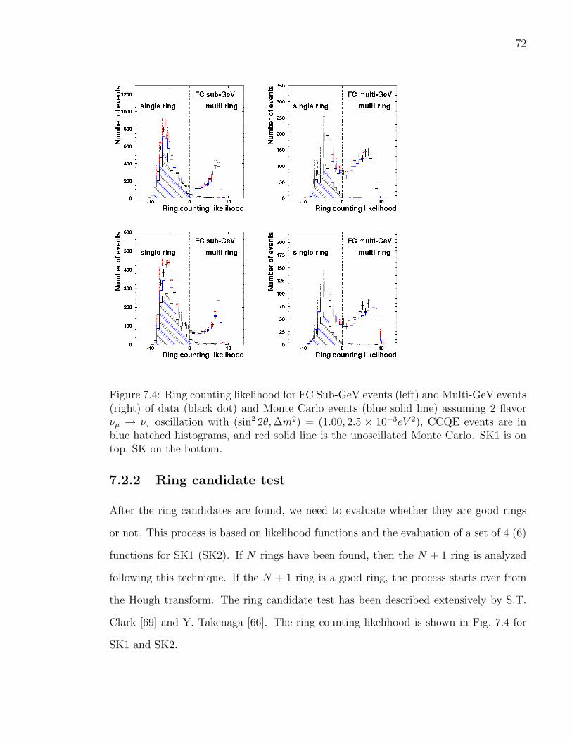
72
Figure 7.4: Ring counting likelihood for FC Sub-GeV events (left) and Multi-GeV events(right) of data (black dot) and Monte Carlo events (blue solid line) assuming 2 flavorνµ → ντ oscillation with (sin2 2θ,∆m2) = (1.00, 2.5 × 10⁻³eV 2), CCQE events are inblue hatched histograms, and red solid line is the unoscillated Monte Carlo. SK1 is ontop, SK on the bottom.
7.2.2 Ring candidate test
After the ring candidates are found, we need to evaluate whether they are good rings
or not. This process is based on likelihood functions and the evaluation of a set of 4 (6)
functions for SK1 (SK2). If N rings have been found, then the N + 1 ring is analyzed
following this technique. If the N + 1 ring is a good ring, the process starts over from
the Hough transform. The ring candidate test has been described extensively by S.T.
Clark [69] and Y. Takenaga [66]. The ring counting likelihood is shown in Fig. 7.4 for
SK1 and SK2.

73
Figure 7.5: Example 1 GeV muon (left) and 1 GeV electron (right), in the SK1 detector.
7.3 Particle Identification (sppatid)
The goal of the particle identification is to determine the type of a particle. Knowing the
flavor of the lepton emitted during the neutrino interaction is useful to determine the
flavor eigenstate of the neutrino at the time of the interaction. Electron events create
electro-magnetic showers and therefore the Cherenkov rings produced by electrons tend
to by “fuzzy”. Muon events, on the other hand, do not create showers, and their rings
tend to have a very clear edge. The particle identification algorithm is based on these
ring properties and classifies events into 2 categories: e-like and µ-like. Electrons and
photons produce e-like events while muons and other heavy particles such as pions or
kaons produce µ-like events. In addition, while electrons and photons produce Cherenkov
rings with an opening angle of 42, muons and other heavy particles can produce rings
with a slightly smaller opening angle if they are not highly relativistic. This feature
will also be used for the identification of protons presented in Appendix D, which also
describes the selection of a CCQE sample. An example of e-like and µ-like events are
presented in Fig. 7.5. The rate of mis-identification is computed using cosmic ray muons
that decay in the detector, therefore provided a good sample of both muon and electron
events.
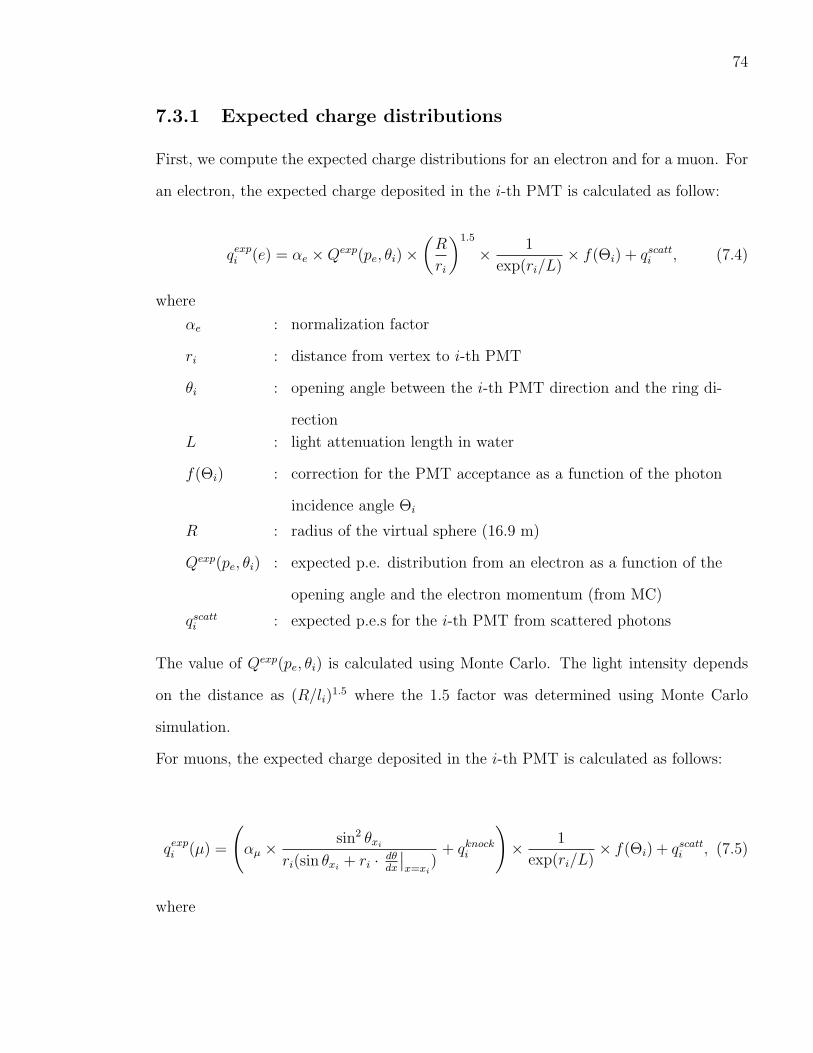
74
7.3.1 Expected charge distributions
First, we compute the expected charge distributions for an electron and for a muon. For
an electron, the expected charge deposited in the i-th PMT is calculated as follow:
qexpi (e) = αe ×Qexp(pe, θi)×(R
ri
)1.5
× 1
exp(ri/L)× f(Θi) + qscatti , (7.4)
where
αe : normalization factor
ri : distance from vertex to i-th PMT
θi : opening angle between the i-th PMT direction and the ring di-
rection
L : light attenuation length in water
f(Θi) : correction for the PMT acceptance as a function of the photon
incidence angle Θi
R : radius of the virtual sphere (16.9 m)
Qexp(pe, θi) : expected p.e. distribution from an electron as a function of the
opening angle and the electron momentum (from MC)
qscatti : expected p.e.s for the i-th PMT from scattered photons
The value of Qexp(pe, θi) is calculated using Monte Carlo. The light intensity depends
on the distance as (R/li)1.5 where the 1.5 factor was determined using Monte Carlo
simulation.
For muons, the expected charge deposited in the i-th PMT is calculated as follows:
qexpi (µ) =
(αµ ×
sin2 θxiri(sin θxi + ri · dθdx
∣∣x=xi
)+ qknocki
)× 1
exp(ri/L)× f(Θi) + qscatti , (7.5)
where

75
αµ : normalization factor
x : track length of the muon
xi : track length of the muon at which Chrenkov photons are emitted
toward the i-th PMT
θ : Cherenkov opening angle of the muon traveling at x
θi : Cherenkov opening angle of the muon traveling at xi
qknocki : expected p.e.s for the i-th PMT from knock-on electrons
The sin2 θ factor comes from the fact that the Cherenkov light intensity depends on
the Cherenkov angle. The contribution of knock-on electrons is estimated using Monte
Carlo simulation.
7.3.2 Estimation of particle type
There are two types of particle type estimators. One estimator relies on the expected
charge pattern described in the previous sub-section, while the other relies on the Che-
renkov angle. For the pattern estimator, we first construct a likelihood for each ring, as
described in the following equation:
Ln(e or µ) =∏
θi<(1.5×θc)
prob
(qobsi , qexpi (e or µ) +
∑n′ 6=n
qexpi,n′
), (7.6)
where the product is made over the PMTs inside the n-th ring. qobsi is the observed
number of photo-electrons in the i-th PMT, qexpi,n (e or µ) is the expected number of
photo-electrons in the i-th PMT from the n-th ring assuming an electron or a muon as
in Eq. 7.4 or Eq. 7.5, and qexpi,n is the expected number of photo-electrons from the n′-th
ring without any assumption of particle types. The function prob is the probability to
detect qobsi in the i-th PMT when qexpi is expected.
To combine this pattern estimator with the angle estimator, we convert it into a χ2
parameter:

76
χ2n(e or µ) = −2 logLn(e or µ) + constant. (7.7)
Once we have the χ2 parameter, we compute a probability as done in the following
equation:
P patternn (e or µ) = exp
(−(χ2(e or µ)−min [χ2
n(e), χ2n(µ)])2
2σ2χ2n
), (7.8)
where σ2χ2n
is the resolution of the χ2 distribution and is equal to σ2χ2n
=√
2N and N is
the number of PMTs used in the calculation.
To use the Cherenkov angle estimator we compute the following probability:
P anglen (e or µ) = exp
(−(θobsn − θexpn (e or µ)
)2
2(δθn)2
), (7.9)
where θobsn is the reconstructed opening angle of the n-th ring, δθn its error and θexpn is
the expected opening angle of the n-th ring assuming the particle is either a electron or
a muon.
Once both probabilities are computed we can build the final PID probability. For
single ring events we use both the pattern and the angle probability while for multi-
ring events we use only the pattern probability. Therefore for single-ring events we
have P1((e or µ) = P pattern1 (e or µ) × P angle
1 (e or µ) and for multi-ring events we have
Pn((e or µ) = P patternn (e or µ).
Finally we construct the PID estimator using the following equation:
P =√− logPn(µ)−
√− logPn(e). (7.10)
The PID estimator is shown in Fig. B.7 for SK1 and Fig. B.8 for SK2. The systematic
uncertainties on the PID estimator are 1% for the single-ring events and 10% for the
multi-ring events, for both SK1 and SK2.

77
7.4 Precise vertex fitting
For single-ring events, the vertex calculated by TDC-fit in Section 7.1 is not as good
in the direction in which the particle is traveling as it is in the perpendicular plan to
that direction. This is because if the vertex is slightly moved along the longitudinal
direction the time of flight calculated for each hit PMT will be moved by the same
amount, and therefore the goodness of fit does not change by much. In order to solve
this problem, we apply a different fitter called MS-fit (msfit) (muon shower fit). MS-
fit is based on a likelihood comparing the observed charge distribution and a expected
charge distribution, similar to what is done in the PID algorithm. Using the same
likelihood function as in Eq. 7.6 we modify slightly the vertex and the ring direction,
maximize the goodness of TDC-fit, and iterate until the vertex moves by less than 5cm
and the ring direction by less than 0.5.
The vertex resolution and angular resolution for different sub-samples and for SK1
and SK2 are shown in Table 7.1 and in Fig. 7.6, Fig. 7.7, Fig. 7.8, and Fig. 7.9. The
resolution is defined as the width at which 68% of events are included.
SK1 SK2e-like µ-like e-like µ-like
Vertex resolutionSub-GeV single ring 27 cm 26 cm 32 cm 31 cmMulti-GeV single ring 49 cm 24 cm 47 cm 27 cmMulti rings - 57 cm - 77 cmPC events 56 cm 63 cm
Angular resolutionSub-GeV 3.1 2.0 3.3 2.2
Multi-GeV 1.5 0.9 1.5 1.0
Table 7.1: Vertex resolution and angular resolution for SK1 and SK2.

78
Figure 7.6: Distance between the true and reconstructed vertex for SK1. Top row: FCSub-GeV 1ring e-like, FC Sub-GeV 1ring µ-like, FC multi-ring µ-like. Bottom row: FCMulti-GeV 1-ring e-like, FC Multi-GeV 1ring µ-like, PC
7.5 Momentum determination (spfinalsep)
The momentum calculation of each ring is based on the observed number of photoelec-
trons inside a cone of 70 opening angle around the ring (variable RTOT ). When two
rings intersect, we have to properly assign the number of p.e’s that belong to each ring.
To do so, we use the expected charge contribution from each ring (sum on index n′) in
the i-th PMT and we compute the fractional charge observed from the n-th ring in the
i-th PMT:
qobsi,n = qobsi ×qexpi,n∑n′ q
expi,n′. (7.11)
We compute the variable RTOT for each ring based on the number of observed p.e’s
in the cone of 70 opening angle and in a time window that goes from -50 ns to 250 ns

79
Figure 7.7: Distance between the true and reconstructed vertex for SK2. Top row: FCSub-GeV 1ring e-like, FC Sub-GeV 1ring µ-like, FC multi-ring µ-like. Bottom row: FCMulti-GeV 1-ring e-like, FC Multi-GeV 1ring µ-like, PC
around the peak of the “TOF-subtracted” hit timing distribution. We also correct for
the water attenuation length and the acceptance of the PMT. In order to convert RTOT
into the momentum of each ring, we need to know the absolute energy scale. To do so,
we use several calibration methods as described in Section 4.5. The resolution of the
momentum is presented in Fig. 7.10.
7.6 Ring number correction (aprngcorr)
After the momentum reconstruction is done, we apply a correction to the number of
rings found by the ring counting algorithm. This is applied at this stage because mis-
fitted rings often have a low momentum and overlap with other more energetic rings.
Two sets of cuts are applied at this stage. If one of the two sets of cuts is satisfied, then

80
Figure 7.8: Angle between true and reconstructed direction of the outgoing lepton forCC quasi-elastic events for SK1. Top: FC Sub-GeV 1ring e-like, FC Sub-GeV 1ringµ-like. Bottom: Multi-GeV 1-ring e-like, FC Multi-GeV 1ring µ-like.
the ring i is removed. We require either the following set of three cuts,
1. Ei < Ej The visible energy of ring i is smaller than the visible energy of ring j
2. θij < 30 The angle between the direction of ring i and ring j is less than 30
degrees.
3. Ei × cos θij < 60 MeV
or we require the following two cuts.
1. EiPn En
< 0.05
2. Ei < 40 MeV

81
Figure 7.9: Angle between true and reconstructed direction of the outgoing lepton forCC quasi-elastic events for SK2. Top: FC Sub-GeV 1ring e-like, FC Sub-GeV 1ringµ-like. Bottom: Multi-GeV 1-ring e-like, FC Multi-GeV 1ring µ-like.

82
Figure 7.10: Momentum resolution for electron (top) and muon (bottom) for SK1 (filledcircles) and SK2 (open circles).

Chapter 8
Dataset
In this chapter I will describe in details the dataset used for the L/E analysis presented in
Chapter 9. The samples of neutrino events used in the L/E analysis are the following:
the fully-contained events sample and the partially-contained events sample for both
SK1 (1489 days of data) and SK2 (804 days). We classify events further into FC events
with single-ring or multi-ring and PC events which are stopping or through-going. In
all samples, we select only µ-like events.
The main challenge of the L/E analysis is to select a sample of neutrino events with
a good enough resolution in flight length L and energy E so that the oscillation pattern
of νµ → ντ as a function of L/E is not washed out. In order to do so, we reconstruct L
and E in a different way than in the “zenith angle” analysis, and we apply a cut on the
L/E resolution.
For quasi-elastic charged current interaction ν + n → p + e−, our accuracy on the
reconstruction of the energy and the flight length of the neutrino is limited by the fact
that in most cases we do not see the recoiling proton coming from a neutrino interaction.
If we were able to see the recoiling proton, our reconstruction of the energy and flight
length would be more accurate. In some cases, the recoil proton is above Cherenkov
threshold and if it is properly identified, we can collect a sample of events for which all
the kinematics variables are known. In that case, the energy and the flight length of
83

84
the incoming neutrino can be fully reconstructed. This idea was explored and is fully
described in Appendix D. Adding this sample did not improve the sensitivity of the L/E
analysis, and it was therefore not added.
8.1 Events samples
After data reduction, a few more cuts are applied to select FC and PC events which are
suitable for the L/E analysis.
8.1.1 FC single-ring and multi-ring
For both fully-contained sample we apply the following three cuts:
• Inside the fiducial volume. Distance between the reconstructed vertex and the
endcap of the detector is greater than 1.5 m and the distance between the vertex
and the barrel is greater than 1.0 m.
• No more than 10 (16) hits in the outer detector for SK1 (SK2).
• Visible energy greater than 30 MeV.
The fiducial volume used for the fully-contained samples in the L/E analysis is larger
than for other analyses and larger than for the PC samples. This is done to increase the
statistics. The vertex distributions for data and Monte Carlo are shown in Fig. B.1 and
Fig. B.3.
To select FC single-ring events we apply two additional cuts.
• Number of rings equals 1.
• The ring should identified as µ-like and its momentum should be greater then 200
MeV/c (pµ > 200 MeV/c).

85
To select FC multi-ring events, we apply the same three common FC cuts, and then
apply two more cuts:
• Number of rings must be greater than 1.
• The most energetic ring must be µ-like and its momentum must be greater than
600 MeV/c. The visible energy Evis should also be greater than 600 MeV.
8.1.2 PC stopping and through-going
PC stopping events contain muons that stop in the outer detector. The energy of
such muons can be accurately reconstructed since we know the length of the muon,
and therefore we know its energy from calculation of the energy loss via dE/dx. PC
through-going events on the other hand contain muons which exited the outer detector
before stopping, and therefore the energy reconstructed for such events is only a lower
limit on the energy of the incoming muon.
To separate PC stopping from PC through-going events we look at the maximum
number of OD photoelectrons in a 500 ns time window between -400 ns and +500 ns
(PEanti) and for stopping events we require that PEanti be less than 1.5 times the ex-
pected number of photoelectrons from the track length information (PEexp). Figure 8.1
shows the separation criteria between PC OD stopping and PC OD through-going for
SK1 and SK2. We estimate the systematic uncertainty on the separation between PC
OD stopping and PC OD through-going by comparing the data and the Monte Carlo;
we do this separately for the top, barrel and bottom of the detector. The agreement
between data and MC for SK2 is not as good as for SK1 and this is taken into account
in the systematic uncertainties. The systematic uncertainties are therefore different for
SK1 and SK2, the SK1 value is 15%, 11.3%, 7.5% for top, bottom and barrel respec-
tively, while the SK2 value is 19%, 18%, 14%, for top bottom and barrel. We decided to
use different systematic uncertainties for top, barrel and bottom because the response of

86
the outer detector is different for these three regions, because of the different geometry
between the barrel and the endcaps and because of the different PMT types between
the top and the bottom.
In summary, we apply three common cuts to select the PC samples:
• Inside the fiducial volume. The distance from the vertex to the wall must be
greater than 2 m.
• More than 10 (16) hits in the outer detector for SK1 (SK2).
• Visible energy greater than 350 MeV.
Then to select the stopping sample, we apply two additional cuts:
• Have a total number of photoelectrons in the ID greater than 3000 (1500) for SK1
(SK2).
• The most energetic or the second most energetic ring must be µ-like.
• PEanti < PEexp/1.5.
To select the PC through-going sample, we apply the same three general cuts and also
two additional cuts. We do not need to apply a µ-like cut to the PC through-going
sample since already 99% of CC interactions which produce PC through-going events
are νµ + νµ CC interactions. The two additional cuts are:
• Total number of photoelectrons in the ID greater than 3000 (1500) for SK1 (SK2).
• PEanti ≥ PEexp/1.5.

87
Figure 8.1: Separation criteria between PC OD stopping and PC OD through-goingevents for SK1 (left) and SK2 (right). The black dots are the data, the black solid lineis the unoscillated Monte Carlo, the blue solid line is the oscillated Monte Carlo, andthe red hatched histograms are the true stopping events.
8.2 Reconstructing L and E
Reconstructing the energy E and the flight length L as accurately as possible is crucial
for the L/E analysis in order to be able to see the oscillatory pattern. If the resolution
is not good enough, the oscillation averages out.
8.2.1 Energy
To reconstruct the neutrino energy we compute the effective energy (EVIS2) of all the
outgoing charged particle by looking at the energy of their Cherenkov rings in the inner
detector. For PC events, we have to apply a special treatement to estimate the energy
of the muon that was deposited after it exited the inner detector.
Fully-contained single-ring
For single-ring fully contained events, the energy of the charged particles is simply the
reconstructed energy of the outgoing muon EVIS2= Eµ.

88
Fully-contained multi-ring
For fully-contained multi-ring events, we assume that the most energetic ring comes
from a muon emitted through a CC interaction while the other rings are either assumed
to be electro-magnetic showers if they are e-like or pions if they are µ-like. Therefore,
the reconstructed energy of the charged particles is EVIS2= Eµ +∑n
i=2(Eie or Ei
π).
The reconstruction of µ-like rings assumes that the particle is a muon and therefore
the mass of the muon is involved in the energy reconstruction through the Cherenkov
energy threshold. If we believe that the particle which emitted the µ-like ring was
not a muon but some other massive particle we have to correct for this fact. We can
rewrite the energy of a muon as Eµ = (Eµ − Ethµ ) + Eth
µ and the energy of a pion as
Eπ = (Eπ − Ethπ ) + Eth
π , where Ethµ = 160 MeV and Eth
π = 212 MeV are the Cherenkov
energy threshold for a muon and a pion. If we assume that dE/dx in water is independent
from the energy and the particle type, then the number of emitted Cherenkov photons
is just proportional to the track length. So the energy deposited from a muon and
a pion which have been estimated from the same ring satisfy the following relation:
Eµ − Ethµ = Eπ − Eth
π . And therefore: Eπ = Eµ − Ethµ + Eth
π = Eµ + (Ethπ − Eth
µ ). So in
the case of pions we have to correct the observed energy as follows: Eπ = Eµ + 52 MeV.
Partially-contained
For the PC sample, we have to take into account the energy deposited in the dead
layer that separates the inner and outer detectors, and the energy deposited in the
outer detector itself. The energy of the outgoing charged particles is therefore EVIS2=
Einner + Edead + Eouter.
Einner is reconstructed in the same way as for fully-contained single or multi-ring
events, but we have to apply a correction on the number of rings. Because PC events
are quite energetic (≈ 10 GeV), most of the produced rings will be collinear and are likely

89
Figure 8.2: Pµ/Dinner for quasi-elastic (QE) interactions (hatched) and non-QE inter-actions in the atmospheric neutrino MC PC single-ring sample. Events at the right ofthe arrow are divided into two rings: a muon ring and an electron ring.
to overlap. We can recognize mis-reconstructed rings by comparing the momentum of
the ring (Pµ) and its track length in the inner detector (Dinner) for the PC single-ring
sample as in Fig. 8.2. Quasi-elastic events are by definition single-ring events if the
proton is below Cherenkov threshold, while non quasi-elastic are likely to be multi-ring.
The large tail of non quasi-elastic events in Fig. 8.2, is due to overlapping pions and/or
other particles. We therefore apply a correction to the number of rings by using the
following method. If the most energetic muon ring satisfies Pµ/Dinner > 3.0 MeV/cm,
the ring is separated into a muon ring with momentum estimated from the track length
in the ID as Dinner × dE/dx, where dE/dx = 2.4 MeV/cm and an electron ring. The
expected charge from the muon is subtracted from the ring and the remaining charge is
used the reconstruct the momentum of the electron.
Edead is the energy deposited in the dead region that separate the inner detector from
the outer detector. We estimate the energy deposited in this region by measuring the
distance the muon traveled in the dead region and assuming a dE/dX of 2.4 MeV/cm.
Eouter is the energy deposited in the outer detector. The estimation of Eouter is done
in the same way as Edead and the flight length in the OD is computed using the energy

90
of the muon and our Monte Carlo.
Reconstruction of the neutrino energy
Finally, once we have reconstructed EVIS2, we can infer the neutrino energy by doing a
polynomial extrapolation. The parameters a, b, c, d of the polynomial fit are computed
using our Monte Carlo.
Erecν = Evis2 × (a+ bx+ cx2 + dx3) (8.1)
with x = log10(Evis2)
The distributions of (Etrueν −Erec
ν )/Etrueν for each sample is presented in Fig. 8.3 for
SK1 and Fig. 8.4 for SK2. It is also summarized as a function of energy in Fig. 8.5.
8.2.2 Flight Length
The reconstruction of the flight length uses the reconstructed neutrino energy described
in the previous section, the reconstructed zenith angle and it takes into account the fact
that we do not know precisely where in the atmosphere the neutrino is created.
Fully-contained single-ring
For single-ring events, the direction of the neutrino is assumed to be the same as the
direction of the outgoing muon.
Fully-contained multi-ring
For multi-ring events, we assume that the most energetic ring is a muon and that the
other rings are either pions or electro-magnetic showers (from photons or electrons) as
described in the energy reconstruction section. The zenith angle of the incoming neutrino

91
Figure 8.3: (Etrueν − Erec
ν )/Etrueν distributions for µ-like SK1 events. Top left: FC Sub-
GeV 1 ring. Bottom left: FC Sub-GeV multi-ring. Top middle: FC Multi-GeV 1 ring.Bottom middle FC Multi-GeV multi-ring. Top right: PC stopping. Bottom right PCtrough-going. The region histograms represents 68% of the events. Note: the resolutioncut has not yet been applied.
is simply equal to the weighted sum of all the reconstructed rings: cos θν = cos θsum,
with ~dsum = pµ · ~d1 +∑n
i=2(pie or piπ) · ~di.
Partially-contained sample
The zenith angle of PC events is computed in a very similar way as for FC events. For
single-ring events, we have cos θν = cos θµ. And for multi-ring events we use cos θν =
cos θsum, with ~dsum = α ·pµ · ~d1 +∑n
i=2(pie or piπ) · ~di. The numerical factor α is set to 2.0
for stopping events and 4.0 for through-going events. This factor has been introduced
for better performance.
The angular resolution for each sample is presented in Fig. 8.6 for SK1 and Fig. 8.7

92
Figure 8.4: (Etrueν −Erec
ν )/Etrueν distributions for µ-like SK2 events. Top left: FC Sub-
GeV 1 ring. Bottom left: FC Sub-GeV multi-ring. Top middle: FC Multi-GeV 1 ring.Bottom middle FC Multi-GeV multi-ring. Top right: PC stopping. Bottom right PCtrough-going. The region histograms represents 68% of the events. Note: the resolutioncut has not yet been applied.
Figure 8.5: Energy resolution for SK1 (left) and SK2 (right).

93
Figure 8.6: Angle between true and reconstructed neutrino direction for µ-like SK1events. Top left: FC Sub-GeV 1 ring. Bottom left: FC Sub-GeV multi-ring. Topmiddle: FC Multi-GeV 1 ring. Bottom middle FC Multi-GeV multi-ring. Top right:PC stopping. Bottom right PC trough-going. The hatched region represents 68% of theevents. Note: The resolution cut has not yet been applied.
for SK2. It is presented as a function of energy in Fig. 8.8.
Reconstruction of the neutrino flight length
Finally after the reconstruction of the neutrino zenith angle has been completed, we
estimate its flight length. The relation between zenith angle and flight length can be
seen in Fig. 8.9. For horizontal events (cos θ = 0) a small variation in the zenith angle
represents a large variation in the flight length, therefore it is very hard to obtain a
good resolution on the flight length for horizontal events. For upward going events, the
uncertainty in the production height is of the order of a percent at most since the overall
flight length is large (≈ 10000 km) while the atmosphere is only about 15 km thick, but

94
Figure 8.7: Angle between true and reconstructed neutrino direction for µ-like SK2events. Top left: FC Sub-GeV 1 ring. Bottom left: FC Sub-GeV multi-ring. Topmiddle: FC Multi-GeV 1 ring. Bottom middle FC Multi-GeV multi-ring. Top right:PC stopping. Bottom right PC trough-going. The region histograms represents 68% ofthe events. Note: the resolution cut has not yet been applied.
Figure 8.8: Angular resolution for SK1 (left) and SK2 (right).

95
Figure 8.9: True flight length versus true zenith angle for fully-contained single-ringevents with an Evis between 0.9 and 1.1 GeV (SK1 Monte Carlo).
for downward and horizontal going events the uncertainty is much larger, and this is
taken into account in the systematic erros.. We estimate the neutrino flight length by
using the reconstructed zenith angle, the neutrino energy, and assuming νµ interactions.
8.3 Resolution cut
In order to perform the L/E analysis, we have to select a set of events that have a good
resolution in L/E. To do so, we use Monte Carlo to predict the L/E resolution of each
sample (FC-1R, FC-MR, PC-stop and PC-through) at each point of a (cos θrecν , Erecν )
grid. Later, we keep only events that are expected to have a good resolution.
In order to to estimate the resolution as accurately as possible, we take into account
the fact that the Lν/Lrecν and Eν/E
recν have asymmetric distributions and that the
peak of the (Lν/Eν)/(Lrecν /Erec
ν ) distribution is not equal to one. Since this smears

96
the resolution, by correcting for this known fact, we can improve the resolution of each
sample. To do so we shift the L/E value as follow: (Lrecν /Erecν )′ = δ(L/E)× (Lrecν /Erec
ν )
where δ(L/E) is computed for each sample using Monte Carlo and for each point on
the (cos θrecν , Erecν ) grid. Once this is done, we can draw a resolution map and this is
shown in Fig. 8.10. We decided to use the 70% cut as this was found to maximize the
log likelihood [47].
The effect of the resolution is to remove events coming from the horizontal direction
as for these events a small variation in θ corresponds to a large variation in flight length.
Very high energy events (Evis2 > 10 GeV for FC single-ring and Evis2 > 50 GeV for
FC multi-ring and PC events) are also removed as we do not have enough statistics to
estimate their resolution. The log10((Lν/Eν)/((Lrecν /Erec
ν )) distributions are shown in
Fig. 8.11. The effect of the resolution cut can be seen in Fig. 8.12.
8.4 Event summary
The dataset obtained after the resolution cut is applied, is presented in Table 8.1. The
energy of the events range from 30 MeV to about 20 GeV, the flight length ranges
from a few kilometers to about 10000 km. Close to the horizontal, the flight length
changes fast as a function of the zenith angle, therefore L/E bins which consists mainly
of events coming from an horizontal direction have much less statistics that others.
Furthermore, the flight length resolution is usually worse for horizontal events, and this
decreases even further the statistics of these bins. As a consequence, the distribution
of the number of events as a function of L/E has the “two-bumps” structure that can
be seen in Fig. 8.13. Using ∆m223 = 2.2 × 10⁻³ eV 2, the first oscillation minimum is
located where L/E = π2/(1.27 × ∆m2) = 562 km/GeV . At this value of L/E, most
of the events come from the PC through-going sample. Therefore, the work done on
improving PC reduction and consequently increasing the PC sample statistics, will be
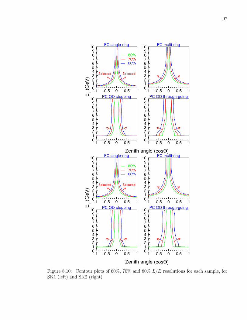
97
Figure 8.10: Contour plots of 60%, 70% and 80% L/E resolutions for each sample, forSK1 (left) and SK2 (right)

98
Figure 8.11: log10((Lν/Eν)/((Lrecν /Erec
ν )) distributions for FC single-ring, FC multi-ring,PC OD stopping and PC OD through-going without the resolution cut (dashed lines)and with the resolution cut (solid lines).
Figure 8.12: Effect of the resolution cut: L/E distribution for normalized oscillatedSK1+SK2 Monte Carlo with (red) and without (black) the resolution cut.

99
especially relevant to the L/E analysis when the SK3 sample will be introduced.
SK1 (1489 days) Data MC νµCCApply resolution cut yes no yes noFCSingle-ring 1562 [4491] 2093.6 [6018.1] (98.2%)Multi-ring 445 [667] 625.6 [972.9] (93.5%)
PCStopping 100 [134] 148.5 [193.1] (94.9%)Through-going 445 [710] 670.6 [952.7] (99.2%)
SK2 [804 days] Data MC νµCCApply resolution cut yes no yes noFCSingle-ring 855 [2390] 1170.4 [3306.5] (98.2%)Multi-ring 246 [412] 333.4 [516.6] (93.3%)
PCStopping 73 [98] 68.5 [91.1] (94.2%)Through-going 191 [308] 321.7 [484.5] (99.3%)
Table 8.1: Summary of the event samples for SK1 and SK2 data.

100
Figure 8.13: Stacked L/E distribution for each sub-sample after the resolution cut isapplied and for an unnormalized oscillated set of Monte Carlo.

Chapter 9
L/E analysis
The goal of the L/E analysis is to be able to see the oscillation pattern expected from
the standard 2-flavor oscillation equation (Eq. 2.9). A similar analysis was conducted
by the Soudan-2 experiment [70]. In an ideal case, this oscillation pattern looks like
Fig. 9.1. Because of finite energy and flight length resolution, the oscillatory signature
of the survival probability of muon neutrinos is a challenge to see.
Figure 9.1: Survival probability of νµ → ντ , without any detector effect as a function ofL/E.
101

102
After selecting events as explained in the previous chapter, we apply a maximum
likelihood analysis to determine the best fit oscillation parameters sin2 2θ23 and ∆m223.
Other theories, like neutrino decay [71, 72] or neutrino decoherence [73] predict a deficit
of upward-going neutrinos, but the sinusoidal pattern of neutrino oscillation is unique.
Therefore comparing the L/E spectrum of the data and the L/E spectrum of these
different theories is a good way to determine which model describes the neutrino data
the best.
9.1 Maximum likelihood analysis and χ2 fit
The L/E analysis is performed with a binned maximum likelihood analysis. We use
43 L/E bins ranging from log10(L/E) = 0.0 to 4.3. The systematics used for the
L/E analysis are described fully later in this chapter and are taken into account in the
likelihood using the “pull method” [74]. Because of the small number of events per
L/E bins, Poisson statistics is used. With pull term added for systematic errors, the
likelihood is defined as follows:
L(Nexp, Nobs) =∏i
exp(−N expi )(N exp
i )Nobsi
N obsi !
×∏j
exp
(εj
σsysj
). (9.1)
We can rewrite the likelihood function as a χ2:
χ2 ≡ −2 ln
(L(N obs, N exp)
L(N obs, N obs)
)=
nbin∑i=1
[2(N exp
i (1 +
nsys∑j=1
f ij · εj)−N obsi )− 2N obs
i ln( N obs
i
N expi (1 +
∑nsysj=1 f
ij · εj)
)]+
nsys∑j
(εj
σsysj
)2, (9.2)

103
where N obsi is the number of observed events in the i-th L/E bin, N exp
i is the expected
number of events in the i-th L/E bin from the Monte Carlo simulation and for a given
set of oscillation parameters. N expi can be corrected to account for systematic uncer-
tainties: σsysj is the j-th systematic error and εj is the pull value on the j-th systematic
uncertainty. The f ij parameter is the fractional change expected in the i-th bin from the
j-th systematic due to a variation of the parameter εj.
Searching numerically for the best fit parameters in εk, ∆m2 and sin2 2θ would be
very slow. Instead, we minimize Eq. (9.2) as a function of εk and then, since εk is small,
we can do a linear expansion and obtain a set of linear equations which are much faster
to solve:
nbin∑i=1
[(1 + (f ij · εj)2 + ...)N obs
i −Nexpi
]· f ik =
nsys∑j=1
( δjk(σsysj )2
+nbin∑i=1
N obsi f ijf
ik
)εk. (9.3)
where the number of L/E bins is nbin ≡ 43 and the number of systematic errors is
nsys ≡ 29. We then scan the ∆m2 and sin2 2θ parameter space in order to find the
set of parameters that finally minimize the reduced χ2. It is worth noticing that this
approach is completely equivalent to doing a unbinned maximum likelihood analysis if
we use the Monte Carlo to generate the p.d.f. P needed in the following equation. The
proof can be found in Appendix C.
lnL =
Nobs∑i
ln(N exp · P (xi|α))
−N exp
(9.4)

104
9.1.1 Combining SK1 and SK2 dataset
When combining datasets corresponding to different versions of the detector (like the
SK1 and the SK2 datasets), we have to make sure that the systematic errors are taken
into account correctly. Some systematic errors are common to both datasets, like the
uncertainties on the neutrino flux, while others are different for each datasets, like the
uncertainties directly related to the detector, or the algorithms used in the data analysis.
So in order to treat these systematic errors properly, we modify the reduced χ2 defined
earlier as follows:
nbin∗nset∑i=1
(N obsi −N
expi
)f ik =
nsystot∑j=1
(δjkσ2j
+nbin∗nset∑
i=1
N obsi f ijf
ik
)εk, (9.5)
with nset ≡ 2 since we have two datasets (SK1 and SK2), and the total number of sys-
tematic uncertainty being nsystot = nsyssk1+nsyssk2+nsyscommon, where nsyscommon =
13 and nsyssk1 = nsyssk2 = 16 so nsystot = 45. By doing this, we allow pull terms re-
lated to uncertainties that are different between SK1 and SK2 to vary separately while
pull terms related to uncertainties that are common between SK1 and SK2 can take
only a single value.
To apply this method, we modify the fij matrix such that the terms corresponding
to an SK1-only systematic and an SK2 bin (and vice versa) are set to zero, while terms
that are common to SK1 and SK2 are forced to be identical. A schematic view of the
changes made to the fij matrix is presented in Table 9.1. This method can be extended
to more datasets such as SK1+SK2+SK3.

105
fij Sys for SK1 only Sys for SK2 only Sys common to SK1 and SK2x x x 0 0 0 a b c d
SK1 x x x 0 0 0 e f g hbins x x x 0 0 0 i j k l
x x x 0 0 0 m n o p0 0 0 x x x a b c d
SK2 0 0 0 x x x e f g hbins 0 0 0 x x x i j k l
0 0 0 x x x m n o p
Table 9.1: Schematic view of the fij matrix modified to account for two datasets
9.2 Systematic uncertainties
There are several categories of systematic errors taken into account. Uncertainty in
the neutrino simulation model, uncertainty in the neutrino interaction simulation, un-
certainty in the event reduction, and uncertainty in the event reconstruction. The
systematic uncertainties used in the L/E analysis are a subset of the ones used in the
zenith angle analysis. The description of each systematic, its value for SK1 and SK2,
its best fit values and its pull values are summarized in Tables 9.2, 9.3 and 9.4.
9.2.1 Simulation uncertainties - Neutrino flux
Normalization (1)
The overall normalization is left free because the overall normalization is irrelevant to
the L/E analysis. What is important in the analysis is the shape of the L/E spectrum.
The uncertainty on the overall normalization is linked to the atmospheric neutrinos flux
and it comes from the uncertainty on the cosmic ray flux and the hadronic interaction
used in the model. The normalization is common for SK1 and SK2.

106
Systematic Description common to SK1 and SK2σ % best fit% pull
1 Normalization free 0.14 0.000Neutrino flux
3 Flux νµ/νµ ratio 6.0 0.49 0.00664 Flux up/down 0.06 0.0032
Single-ring < 400 MeV 0.3Single-ring > 400 MeV 0.5Single-ring multi-GeV 0.2Multi-ring Sub-GeV 0.2Multi-ring Multi-GeV 0.2PC 0.2
5 Flux horizontal/vertical 0.27 0.0726Single-ring < 400 MeV 0.1Single-ring > 400 MeV 1.9Single-ring multi-GeV 2.3Multi-ring Sub-GeV 1.3Multi-ring Multi-GeV 1.5PC 1.7
6 Neutrino flight length 10.0 -0.23 0.00057 Energy spectrum 5.0 -1.47 0.8598 Sample-by-sample multi-GeV (SK1) 5.0 -1.68 0.11328 Sample-by-sample multi-GeV (SK2) 5.0 0.48 0.00922 FC multi-GeV µ / PC (SK1) 6.0 0.01 0.00022 FC multi-GeV µ / PC (SK2) 5.0 -0.01 0.000326 Solar activity (SK1) 20.0 -1.89 0.08926 Solar activity (SK2) 50.0 -7.25 0.0210
Table 9.2: Definition of systematic uncertainties related to the neutrino flux. Theirvalues, best fit values, pull values.
Flux of νµ/νµ ratio (3)
The systematic on the anti-neutrino to neutrino ratio comes from the π+/π− ratio in
hadronic interaction in the flux calculation. This systematic is common to both SK1
and SK2, and is set to 6%.

107
Systematic Description common to SK1 and SK2σ % best fit% pull
Neutrino interaction9 QE cross section 10.0 8.02 0.642510 Single-π 10.0 -1.38 0.019011 DIS cross section 5.0 -1.67 0.111612 Coherent π 100.0 -4.49 0.02013 NC/(CC) 20.0 1.94 0.009421 Nuclear effect 30.0 14.1 0.002224 MA in QE and single-π 20.0 -4.48 0.50125 DIS (Bodek correction) 20.0 24.45 1.494627 Single-meson π0/π+ + π− 40.0 -2.30 0.033
Table 9.3: Definition of systematic uncertainties related to the neutrinos interactiontheir values, best fit values, pull values.
Flux of upward going neutrinos versus downward going neutrinos (4)
The uncertainty in the up/down ratio is due to the fact that the ratio is asymmetric
below a few GeV due the geomagnetic field of the earth, while above a few GeV the
ratio is symmetric. This systematic is common to both SK1 and SK2, and it is energy
dependent. It is set to 0.3% and 0.5% for single-ring sub-GeV events with Evis < 400
MeV and Evis > 400 MeV respectively; to 0.2% for all other types or events.
Flux of horizontal versus vertical neutrinos (5)
The uncertainty in the horizontal/vertical ratio is estimated from the difference in the 3-
D calculation methods described in the simulation chapter. This systematic is common
to both SK1 and SK2, and it depends on the event type. It is set to 0.1% and 1.9% for
single-ring sub-GeV events with Evis < 400 MeV and Evis > 400 MeV respectively; to
2.3% for FC single-ring multi-GeV events; to 1.3% and 1.5% for FC multi-ring sub-GeV
and multi-GeV respectively, and to 1.7% for PC events.

108
Systematic Description SK1 SK2σ best fit pull σ best fit pull
Reconstruction16 Ring counting 0.14 0.0002 -0.86 0.0073
Single-ring < 400 MeV 0.7 2.3Single-ring > 400 MeV 0.7 0.7Single-ring multi-GeV 1.7 1.7Multi-ring Sub-GeV 4.5 8.2Multi-ring Multi-GeV 4.1 0.8
17 Particle ID 1ring -0.01 0.0001 -0.02 0.0002Single-ring sub-GeV -0.1 -0.4Single-ring multi-GeV -0.2 -0.1
18 Particle ID multi ring 0.26 0.0007 1.27 0.0160Multi-ring Sub-GeV -3.9 -2.2Multi-ring Multi-GeV -2.2 -3.4
19 Energy calibration 1.1 -0.14 0.0167 1.70 0.11 0.004320 Up-down asym of E calib 0.6 0.21 0.1177 0.60 0.07 0.14723 PC stop/through top 15.0 0.71 0.0023 19.00 -0.20 0.000128 PC stop/through bottom 11.3 -0.94 0.0069 18.00 -2.08 0.013329 PC stop/through barrel 7.5 0.56 0.0057 14.00 0.33 0.0006
Reduction14 FC reduction 0.2 0.00 0.0000 0.20 0.00 0.000215 PC reduction 2.4 -0.06 0.0007 4.80 -1.42 0.086922 Non-ν BG (µ-like) 0.00 0.0000 0.02 0.0005
Cosmic ray FC sub-GeV 0.1 0.1Cosmic ray FC multi-GeV 0.1 0.1Cosmic ray PC 0.2 0.7
Table 9.4: Definition of systematic uncertainties related to the reconstruction andreduction. Their values, best fit values, pull values.
Neutrino flight length (6)
The production height of a neutrino in the atmosphere is impossible to reconstruct
on an event-by-event basis using the zenith angle, but it can be simulated statistically
using the Monte Carlo. The uncertainty on the production height depends on the zenith
angle. For upward going neutrinos, the systematic error on the neutrino flight length
is only of the order of 1% because the uncertainty in the production height is small
compared to the overall flight length. But for a downward-going or horizontal neutrino

109
the production height of the neutrino matters significantly. The uncertainty is related to
the structure of the atmosphere. To estimate the uncertainty the simulation calculation
is done by changing the density structure of the atmosphere by 10% and observing how
the production height changes as a function of the zenith angle. It is common to both
SK1 and SK2, and is evaluated to be 10%.
Energy spectrum (7)
The spectrum of primary cosmic rays can be well fit with an Eγ form up to where the
spectral index γ is set to -2.74. The systematic in the spectral index is common to both
SK1 and SK2, and is set to 5%.
Sample-by-sample FC multi-GeV normalization (8)
Different flux calculations predict different energy dependence that cannot be explained
by a simple spectral index uncertainty. We therefore compare the number of events
predicted by the Honda [44] flux model to the number of events predicted by other
models (Fluka [45], Bartol [46]) and we assign a 5% systematic error for samples which
include multi-GeV events since all three flux predictions agrees very well below 1 GeV
as shown by G.Mituska [6]. This systematic is calculated separately for SK1 and SK2.
FC multi-GeV µ-like events versus PC normalization (2)
The PC sample also contains multi-GeV events and therefore an uncertainty on its
normalization should be applied as for the FC multi-GeV sample. But the uncertainty
on the PC sample normalization is highly correlated to the uncertainty on the FC multi-
GeV sample normalization. To account for this correlation we use a systematic error on
the ratio of FC multi-GeV µ-like events to PC events. This systematic error is different
for SK1 and SK2 because the software used treat SK1 and SK2 was different. The SK1
value is 6% while the SK2 value is 5%

110
Solar activity (26)
The primary flux of cosmic rays and therefore the atmospheric neutrino flux is affected
by the solar activity as described in Section 5.1. We assign the change in neutrino flux
for ±1 year as the uncertainty related to solar activity. This systematic error is different
for SK1 and SK2 since the ±1 change leads to different uncertainties depending on the
stage of the solar cycle. The SK1 value is 20% while the SK2 value is 50%.
9.2.2 Simulation uncertainties - Neutrino Interactions
The cross-sections involved in neutrino interactions are measured by several experiments
and theoretically predicted. We use these measurements/predictions to estimate this set
of systematic errors. All systematic errors related to neutrino interactions are common
for the SK1 and SK2 dataset. A detailed description of the systematic errors linked to
neutrino interactions can be found in G.Mitsuka’s thesis [6].
9.2.3 Reconstruction uncertainties
Number of rings (16)
The number of rings in one event is reconstructed using a ring counting likelihood as
explained in Section 7.2. The single-ring/multi-ring separation uncertainty is estimated
by comparing the ring counting likelihood between data and Monte Carlo. This system-
atic is considered separately for SK1 and SK2 and is sample and energy dependent, as
it can be seen in Table 9.4.
Particle identification for the FC 1-ring sample (17) and multi-ring sample
(18)
The type of an event (e-like or µ-like) is determined using a PID likelihood as explained
in Section 7.3. The systematic errors related to the particle identification algorithm are

111
estimated by comparing the PID likelihood between data and Monte Carlo. Both errors
are separate for SK1 and SK2, and are different for each sample. The values can be
found in Table 9.4. The minus signs are important when the e-like sample is used to
account for correlation properly. In the L/E analysis, we use only the µ-like sample,
but I decided to keep the minus signs for coherence with the zenith angle analysis.
Energy calibration (19)
The energy calibration is computed by different means depending on the energy region,
as described in Section 4.5. The summary of the energy calibration results is presented
in Fig. 9.2 This systematic is separate for SK1 and SK2, the SK1 value is 1.1% while
the SK2 value is 1.7%.
Up-down asymmetry of energy calibration (20)
The difference in energy scale for upward-going events compared to downward-going
events is calculated using decay electrons from stopping cosmic ray muons. These events
are good for calibration because their vertices are distributed all over the fiducial volume
of the inner detector and the momentum distribution is almost uniform in all directions.
The up/down asymmetry is separate for SK1 and SK2, but both values are set to 0.6%.
PC stopping to through-going (23, 28 29)
The separation between stopping PC events and through-going PC events is estimated by
comparing data and Monte Carlo. We look at the distribution of the observed numbers
of photoelectrons in the OD (PEanti) divided by the expected number of photoelectrons
(PEexp). We fit the distributions of PEanti/PEexp for both data and Monte Carlo to find
the means of each distribution. We then shift the MC sample by meandata/meanmc, and
count how many events classified as stopping before the shift would become through-
going. The number of changing events divided by the total number of stopping events is

112
Figure 9.2: Summary of the absolute energy scale calibration for SK1 (top) and SK2(bottom). The horizontal axis shows the momentum range of each source and thevertical axis shows the deviation of the data from the Monte Carlo predictions. [6].

113
Figure 9.3: The uniformity of the detector gain as a function of zenith angle for SK1(left) and SK2 (right). The vertical axis in the two figures are the averaged momentumof decay electron events [6].
the systematic uncertainty. Because there are two types of OD PMTs and because most
of the old IMB tubes are on the top of the detector while most of the new ones are in
the bottom, we estimate this systematic error separately for the top, barrel and bottom
of the detector. An example of the PEanti/PEexp distribution for the SK1 barrel is
shown in Fig. 9.4, in that case 260 events were moved from PC stopping to PC through-
going when the shift was applied, so the systematic uncertainty for the SK1 barrel is
260/3463=0.075. This systematic is separate for SK1 and SK2, the SK1 value is 15%
, 11.3 % , 7.5 % for top, bottom and barrel respectively, while the SK2 value is 19%,
18%, 14%, for top, bottom and barrel.
9.2.4 Reduction uncertainties
FC reduction (14)
The systematic uncertainty on the fully-contained reduction is estimated by studying
the effect of changing the cuts values. This systematic is separate for SK1 and SK2, the
SK1 value is 0.2% while the SK2 value is 0.2%.

114
Figure 9.4: PEanti/PEexp for SK1 barrel. The black dots are the data, the black solidhistogram is the MC before the shift and the red solid histogram is the MC after theshift.
PC reduction (15)
The estimation of PC systematic uncertainty has been described in detail in W.Wang’s
thesis [67], it is largely dominated by the systematic uncertainty on the number of hits in
the outer detector (NHITAC), because NHITAC is the variable used to separate FC events
from PC events. The PC reduction systematic is separate for SK1 and SK2, the SK1
value is 2.4% while the SK2 value is 4.8%.
Non-neutrino background (22)
The non-neutrino background is estimated during the reduction processes as was pre-
sented in Table 6.2 for the background in the fully-contained sample and in Section 6.2.6
for the background in the partially-contained sample. In the L/E analysis, only back-
ground events in the µ-like sample are relevant, and they mainly come from cosmic ray
muons. The systematic error on the background contamination is separate for SK1 and
SK2 and is energy dependent. For SK1 and for SK2, the FC sub-GeV sample and the
FC multi-GeV samples both have a systematic error on the background contamination

115
of 0.1%. The PC sample the systematic is set to 0.2% in SK1 and 0.7% in SK2.
9.3 Results
9.3.1 Dealing with non physical region
The best fit result in sin2 2θ23 that we obtained is larger than one, which is not a physical
result, therefore when drawing the confidence interval we have to correct for that fact.
To do so, we followed the 1996 PDG method [75] to treat results close to a physical
boundary. In this section, I will describe this method for a 1-parameter fit, it can then
be extended for the 2-parameter fit used in the L/E analysis. Assume that the result
of a fit falls in an unphysical region (negative mass, sin θ greater than one, etc...) and
the minimum χ2 value of the fit is χ2min = 0.853. If the fit is forced to give a result in
the physical region, then χ2phys = 1.353. The difference between the two χ2 is ∆χ2 = 0.5
which corresponds to σ = 0.25, and which means that 60% of the gaussian falls in the
unphysical region as shown in Fig. 9.5. In order to compute a confidence level, I have
to consider only the events that falls in the physical region instead of the entire range.
So if I want to compute the 90% confidence level boundary of my hypothetical case, I
have to draw the boundary at 90% of the 40% of events that are in the physical region,
that is to say at 96% of the entire range. Using confidence level tables, I find that 96%
of events corresponds to σ = 1.76 and therefore χ290,corr = 3.10. So the 90% confidence
level boundary is drawn at χ290,phys = χ2
min + χ290,corr = 0.853 + 3.10 = 3.953.
9.3.2 Oscillation results
The results of the L/E analysis for the SK1 (1489 days) and SK2 (803 days) data for
the νµ to ντ hypothesis are presented in this section. For this analysis 500 years of fully-
contained and 500 years of partially-contained Monte Carlo events were used. The SK1

116
Figure 9.5: 1996 PDG method to treat results close to physical boundary.
+ SK2 data are presented in Fig. 9.6 with unoscillated Monte Carlo and the oscillated
(best fit) Monte Carlo overlaid in red on top of the data.
To see the oscillation pattern, we divide the data and the best fit Monte Carlo by
the unoscillated Monte Carlo. The result of this division is shown in Fig. 9.7, with the
theoretical survival probability for comparison.
Finally, the result of the reduced χ2 is shown in Fig. 9.8 and the slices in ∆m223 and
sin2 2θ23 are shown in Fig. 9.9. If we allow the fit to go in the unphysical region, the χ2 is
equal to 77.1 for 83 degrees of freedom, and the best fit parameters are sin2 2θ23 = 1.04
and ∆m223 = 2.2×10⁻³ eV2. If we constrain the fit to lie in the physical region, the χ2 is
equal to 78.2.0 for 83 degrees of freedom, and the best fit parameters are sin2 2θ23 = 1.00
and ∆m223 = 2.2 × 10⁻³ eV2. At 90% confidence level, we have sin2 2θ23 > 0.94 and
1.85× 10⁻³ eV2 < ∆m223 < 2.65× 10⁻³ eV2

117
Figure 9.6: L/E spectrum. Black circles are the SK1+SK2 data, black histogram is theunoscillated Monte Carlo, red is the best fit oscillated Monte Carlo.
9.3.3 Neutrino decoherence and decay
There are other theories that predict the behavior of atmospheric neutrinos, these
non-standard effects have been studied in detail with the Super-Kamiokande data by
W.Wang [67] and G.Mituska [6] in their Ph.D. theses. Neutrino decay and neutrino
decoherence are two such theories. As it can be seen in Fig. 9.10, one form of neutrino
decay and one form of neutrino decoherence predict a deficit of upward-going muon
neutrino but they do not predict an oscillatory pattern. Therefore studying the L/E
spectrum of the atmospheric neutrino data, and comparing it to predictions from these
theories is the best way to constrain these models. Comparing to these theories also
yields a benchmark for determining a significance of our observation of the oscillation
pattern. Comparing against no oscillation gives a very large χ2 difference, but does not
tell us if we resolve the first oscillation minimum. In this section, I present the SK1
+ SK2 results for neutrino decay and neutrino decoherence and compare them to the
neutrino oscillation results.

118
Figure 9.7: Top: Theoretical survival probability. Bottom: Experimental survivalprobability. (black circles are the SK1+SK2 data, red is the best fit oscillated MonteCarlo).

119
Figure 9.8: Contour map of the oscillation analysis for the SK1 + SK2 dataset.
Figure 9.9: Left: Slice in ∆m223. Right: in sin2 2θ23.
9.3.4 Neutrino Decay
Neutrino decay could also explain the deficit of upward going muon neutrinos [71]. In the
Standard Model, neutrinos cannot decay because they are massless, but several models
predict the decay of massive neutrinos. Lower limits on the lifetime of the neutrinos
come from radiative decay channels as τ/m > 15.4 sec/eV, where τ is the lifetime and
m the mass of the neutrino [72]. The effect of neutrino decay on the survival probability

120
Figure 9.10: Top: Theoritical survival probability of muon neutrinos for neutrino oscil-lation, neutrino decay and neutrino decoherence. Bottom: Survival probability for SK1+ SK2 data (black circles) and compared with the best fit results for neutrino oscillation(red), decoherence model (green) and decay model (blue).
of νµ is the following:
P (νµ → νµ) =
[sin2 θ + cos2 θ exp
(−m2
2τ2
LνEν
)]2
(9.6)
If we fit the atmospheric neutrino data with a neutrino decay assumption instead of
a neutrino oscillation assumption, the final χ2 for the SK1 + SK2 dataset is 92.1 for
83 degrees of freedom so the ∆χ2 comparing neutrino decay and neutrino oscillation is

121
13.9, which is 3.7 σ away from the oscillation result.
9.3.5 Neutrino Decoherence
The deficit of upward-going neutrino can also be explained by neutrino decoherence
induced by new physics like quantum gravity [73]. The decoherence of neutrino can
be parametrized by γ = γ0(Eν/GeV )n and in the case where n = −1, the effect on
the survival probability is a deficit of upward-going neutrino but without an oscillation
pattern.
P (νµ → νµ) = 1− 1
2sin2 2θ
[1− exp(−γ0
LνEν
)
](9.7)
If we fit the atmospheric neutrino data with a neutrino decoherence assumption
instead of a neutrino oscillation assumption, the final χ2 for the SK1 + SK2 dataset is
100.4 for 83 degrees of freedom so the ∆χ2 comparing neutrino decoherence and neutrino
oscillation is 22.2, which is 4.7 σ away from the oscillation result.

Chapter 10
Conclusion
In this thesis, I presented the result of the L/E analysis of the atmospheric neutrino data
collected between 1996 and 2005 by the Super-Kamiokande water Cherenkov detector.
There were two data-taking periods during that time, SK1 lasted from 1996 to 2001
and SK2 from 2002 to 2005. We used the fully-contained and partially-contained event
samples with specific resolution cuts to ensure that the oscillatory pattern of the survival
probability of muon neutrinos is not washed out. This analysis demonstrates that the
survival probability of muon neutrinos follows a sinusoidal function as presented in
Fig. 10.1.
Figure 10.1: Experimental survival probability of muon neutrinos. (black circles are theSK1+SK2 data, red is the best fit oscillated Monte Carlo).
122

123
We created a set of Monte Carlo data and by fitting this Monte Carlo to the Super-
Kamiokande detector data assuming 2 flavor oscillation of νµ → ντ , we found that the
allowed regions for the two parameters, sin2 2θ23 and ∆m223, at 90% confidence level are:
0.94 < sin2 2θ23 (10.1)
1.85× 10⁻³ eV2 < ∆m223 < 2.65× 10⁻³ eV2 (10.2)
The minimum χ2 value for the 2 flavor fit is 78.2/83 d.o.f. if we constrain the fit in
the physical region of sin2 2θ23.
The L/E analysis gives a better measurement of ∆m223 than the traditional zenith
angle analysis, as it can be seen in Fig. 10.2. Our central value for ∆m223 is consistent
with the recent MINOS [27] result but MINOS constrains ∆m223 better (see Fig. 10.2).
Atmospheric neutrinos are still currently the best tool to measure the angle sin2 2θ23,
but accelerator neutrinos and experiments like MINOS (and soon T2K), are now more
powerful at measuring the mass splitting ∆m223.
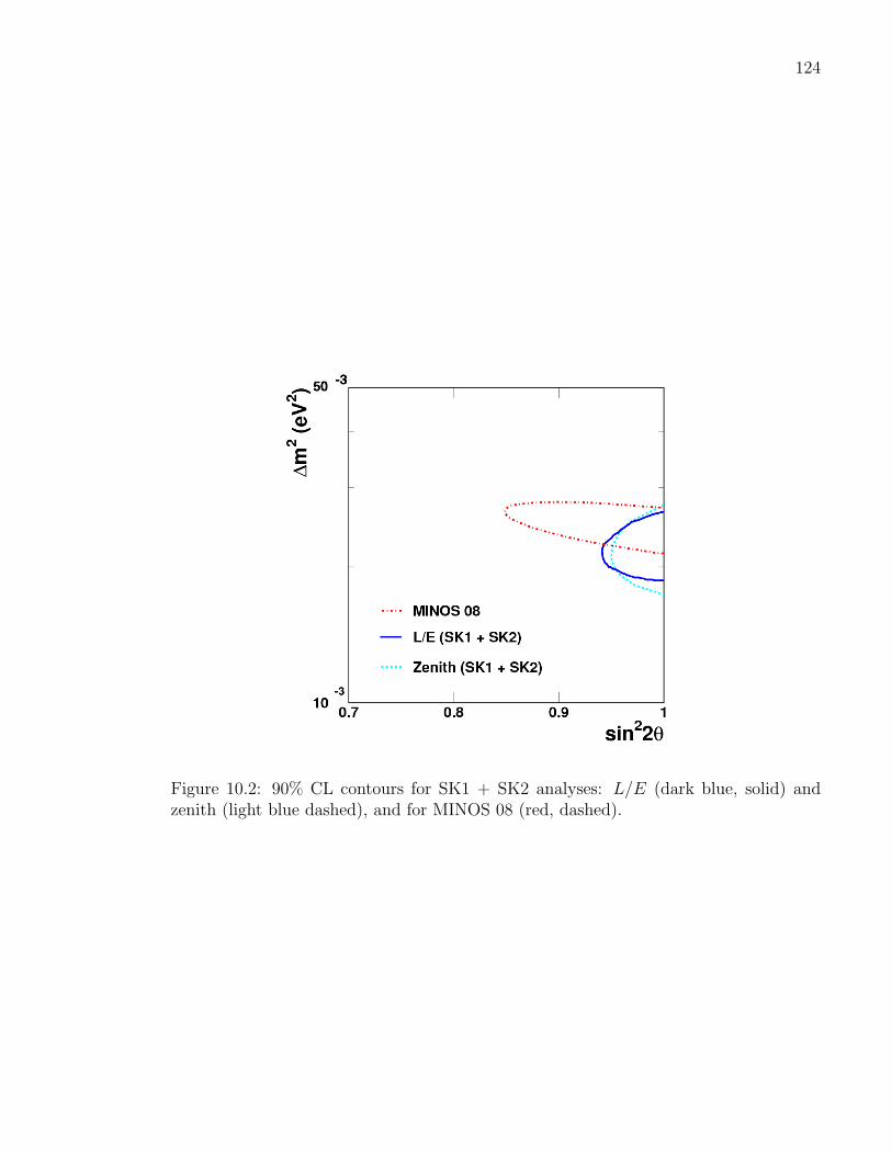
124
Figure 10.2: 90% CL contours for SK1 + SK2 analyses: L/E (dark blue, solid) andzenith (light blue dashed), and for MINOS 08 (red, dashed).

Appendix A
Partially contained data reduction
In this Appendix, I describe the changes made to PC reduction for SK3. During the
reconstruction of the winter 2005-2006, when the full photo-coverage of SK was rebuilt,
we also added a segmentation of the outer detector. This segmentation gives us a new
tool to select partially contained neutrino events. Six months later, we also updated the
computer facilities of SK, and with more processing power, significant improvements to
PC reduction were made possible. The goal of my work was to improve the efficiency of
the PC reduction from 85% to above 97% while keeping the background contamination
as low as possible. The description of PC reduction for the SK1 and SK2 dataset is
done in Chapter 6.
A.1 Purpose of the OD segmentation added for SK3
One of the main modifications of the detector in the SK3 period is the addition of the
OD segmentation. A schematic view of the segmentation is presented in Fig. A.1.
The purpose of the segmentation is to be able to better identify cosmic ray muons
which are clipping the corner of the detector. Figure A.2 shows the distribution of hits
in the wall versus the number of hits in the end-caps (top and bottom of the detector).
125

126
Figure A.1: Schematic view of the OD segmentation (red lines) added in SK3
The top figure is for SK2 and the bottom figure is for SK3. In both cases we keep
events which do not have a high number of hits in both the wall and the end-caps, since
such events are very likely to be corner clipper events. It is clear that adding the OD
segmentation cleaned the region around the cut shown in Fig. A.2 and denoted by the
red line. As a result, the cut is more efficient. Since this cut is applied very early in the
PC reduction process, adding the OD segmentation allowed us to loosen some of the
cuts applied later in the PC reduction process and to gain efficiency in PC reduction
A.2 Modifications to PC reduction for SK3
The purpose of the following modifications was to improve the efficiency of PC reduction.
Since the computer facilities for the Super-K detector were upgraded in 2006, we are
now able to rely much more on CPU-consuming fitters like tfafit used in PC4 and
PC5. Some cuts were removed from PC2 and PC3; PC4 was completely redone and is
now based mainly on the muon fitter muboy. PC5 mainly remains the same as before,
but some cuts were added. The definitions of all the old cuts are not repeated here and
can be found in Section 6.2.
PC1: No modifications except OD segmentation

127
Figure A.2: Number of hits in the OD wall versus number of hits in the OD end-capsbefore segmentation (SK2, top) and after segmentation (SK3, bottom). Events that areabove the red line are corner clippers events and are rejected during PC reduction.
PC2: In PC2, the only modifications were to remove the two cuts that were the biggest
causes of inefficiency.
• numendcap vs numwall (SK-II): Remains the same.
• nouter2: Remains the same.
• nouter: This cut was removed.
• pe200: This cut was removed.
PC3: The flasher cut is the same as before. The ehit8m cut was moved to PC5, see
PC5 section for more information.
PC4:

128
PC4 is now completely based on the muon fitter muboy. Since this is a muon fitter, it will
not give good results for real PC events, but it is very powerful at identifying cosmic ray
muons. One of the features of muboy is that it characterizes each event as either, stopping
muon, through-going muons, multiple muons or corner clipper muons. 96% of PC Monte
Carlo events inside the fiducial volume are classfied as multiple muons, whereas 97% of
background events are classified as either stopping or through-going muons. We will take
advantage of this fact by asking an event to fulfill different conditions depending on what
its muboy classification was. We defined 6 variables which use the muboy information as
defined below.
• muboy angle: This is the angle between the muboy fitted direction and the vector
between the pfit vertex and the center of the highest charge OD cluster. If muboy
angle is less that 90 then the event passes the cut. This cut is designed to remove
cosmic ray muon which stop in the tank.
• muboy dotprod: This cut is similar to muboy angle but instead of using the
center of the highest charged OD cluster, we use the earliest saturated ID pmt.
This is designed to remove both stopping and through-going cosmic ray muons. If
muboy dotprod> −0.8 then an event passes the cut.
• muboy track length: This is the length of the muon track given by muboy. Very
long track length hints toward cosmic ray muons, so events with muboy track
length< 1750 pass this cut.
• muboy goodness: This is the goodness of fit given by muboy. A good fit points
toward a cosmic ray muon, so events with muboy goodness< 0.52 pass this cut.
• muboy corner: This is the distance between the muboy entry point and the corners
of the tank. We ask an event to have muboy corner≥ 300 to pass this cut.

129
• muboy ehit8m: This is similar to the PC3 ehit8m cut, but we use the muboy entry
point instead of the entrance point extrapolated using pfit. An event passes this
cut if muboy ehit8m≤ 10.
If an event is classified as through-going by muboy then it has to pass four out
of the following 5 cuts: Muboy angle, Muboy dotprod, Muboy tracklength, muboy
goodness and muboy corner. If an event is classified as stopping by muboy then it
also has to pass four out of the same set of 5 cuts, but in addition it has to pass the
muboy dotprod cut, and it has to pass either the muboy ehit8m cut or have a muboy
goodness< 0.5. If the event is classified as something else than stopping or through-
going then it only needs to pass two of the set of 5 cuts defined earlier.
Finally we kept the cut on the total ID charge in PC4 but we changed the value of the
cut.
• qismsk: Total charge in the inner detector. This is to remove events with too
little energy in the ID. The cut is now set at 2900.
PC5:
The fast cuts in PC5 remained the same. Most of the slow PC5 cuts remained the same,
but we now classify them between hard cuts and soft cuts. Hard cuts, are cuts that
an event is required to pass in order to be kept. Soft cuts are part of an “all-but-one”
setup. An event may fail zero or one soft cut in order to be kept. This was implemented
in order to improve efficiency, but new cuts had to be introduced in order to remove
background events.
Hard cuts:
• Bye Bye cut
• No ID
• Ano OD

130
• Veto cut
• Angle The value of this cut was change from 90 to 75. The same cut is applied
for the results of both fitter, apfit and msfit.
• Geji cut
• dcorn: (New) This is a new cut which removes an event if the precise fitter
(apfit) vertex is at more than 150 cm from the corner of the tank.
• nncluster cut: (New) This cut uses the nncluster algorithm to count the num-
ber of clusters found in the OD. This cut is used only for very energetic events
(apevis > 20000). In that case, if nncluster finds 2 clusters, the event is rejected.
Soft cuts:
• Cluster cut: (Modified) We modified the cut values to nhit1st< 10 and nhit2nd<
17 .
• Through mu
• New evis
• Stop mu
• St cone
• Evis
• Hits: (Modified) We look at the number of OD hits within 8m of the reconstructed
entry point and in a 500ns time window. The PC5 cut uses apfit to reconstruct
the entry point and the PC3 cut uses pfit. We compared the entry point given by
both fitters and if they are within 1500 cm of each other, we only apply the PC5
version of the cut. If the fitters disagree by more than 1500 cm, then an event has
to pass both the PC3 and the PC5 cuts.

131
• Muboy angle: (New) Since the PC4 criterion is very loose for events which are
not classified as stopping or through-going muons, we use muboy angle again in
PC5.
• Mue decay: (New) For events of very high energy (evis > 25000) we look at the
number of decay electrons found. If no decay electron is found, we reject the event.
A.3 New PC reduction results
The SK3 dataset goes from run 30857 to run 35165, which covers 549.7 days of data.
We also used 60 years of PC Monte Carlo generated with the version of the NEUT
library tagged as 02b. The flux model was used to generate the MC as the 2001 version
of the Honda flux (honda01) but we reweighted the Monte Carlo so that it matched
the predictions of the 2003 version of the Honda flux (honda03). We ran PC reduction
using the version of Super-Kamiokande libraries tagged as 07d. Finally the parameters
related to the outer detector needed by the detector simulated skdetsim were tuned in
May 2007. These parameters were retuned in winter 2009.. A better tuning of the OD
parameters in skdetsim, can decrease systematic uncertainty.
Efficiencies:
After all the modifications described above, Table A.1 shows the old and new PC
reduction efficiencies, using the SK-III dataset and Monte Carlo, and Table A.2 shows
the detail of the final dataset.
PC data:
For the SK3 PC dataset, the final event rate is 0.66±0.03 events per day. The event
rate after each reduction step is shown in Fig. A.3. It is flat which shows that data
taking was running smoothly. The up/down ratio is 0.51 ± 0.07 and the zenith angle
plot is shown in Fig. A.4.

132
SK-III (550 days)Old Eff. (June 07) New Eff (April 08) Data (New reduction)
PC1 99.7% 99.7% 12178704PC2 94.2% 99.2% 4699463PC3 92.8% 99.2% 4692857PC4 85.4 % 98.5% 80417PC5 84.0% 97.1% 663PC5(FV) 78.8% 90.1% 366
Table A.1: PC reduction efficiencies for old and new PC reduction
550 days of data PC BGInside FV 360 6Outside FV 232 65
Table A.2: SK-III Dataset for 551 days of data
BG contamination:
By eye-scanning the final dataset, we found 6 BG events and 366 PC events inside
the fiducial volume in 550 days of data. This corresponds to a BG contamination of
1.6± 0.67%
In order to estimate the BG contamination inside the FV, we fit an exponential to
the dwall (distance from vertex to the wall) distribution of BG events in the whole
SK volume (not only the fiducial volume). The sample of BG events was obtained by
eye-scanning the final data sample, with the corner cut removed in PC5. We had to
remove that cut in order to have a correct estimate of the number of event very close to
the wall. Fig. A.5 shows this fit. Using this method we estimate a BG contamination of
1.9 BG event inside the fiducial volume and therefore a BG contamination of 0.5±0.4%.
A.4 PC reduction systematics uncertainty
In order to compute the systematic uncertainty on the efficiency of PC reduction, we
searched for systematic shifts between data and Monte Carlo in the cut variables.

133
Figure A.3: Event rate for PC SK3 data
In PC2, the only variables that presented a shift was the number of hits in the wall
(numwall). After shifting the cut value to account for the difference between data and
Monte Carlo, and running PC reduction with this new cut value, we obtain a systematic
uncertainty of 0.04%. There was no uncertainty in PC3 since the only active cut in PC3
is the flasher cut.
In PC4, all of the variables presented small shifts between data and Monte Carlo.
Out of 5 variables, 4 had a shift that would decrease the PC efficiency, and one had a shift
that would increase it. We modified the cut variables slightly separately for those two
sets and ran PC reduction again with these modifications to estimate the systematic
uncertainties due to each set. The set of cuts that decreased the efficiency gave a
systematic uncertainty of 0.14%, the set that increased it, gave negligible uncertainty.
For PC5, we treated hard and soft cut differently. For hard cuts, we looked at each
cuts individually and found that only the angle cut had a difference between data

134
Figure A.4: Zenith angle for PC SK3 data (black), oscillated MC (blue), unoscillatedMC (red).
and Monte Carlo, and the systematic associated with this cut was 0.21%. For soft
cuts, we checked the systematic uncertainty associated with all the cuts that increase
efficiency and obtained 0.01%. The systematic uncertainty associated with all the cuts
that decrease efficiency was found to be 0.09%.
In addition to the reduction efficiency, we also computed the uncertainty on the
nhitac (number of hits in the OD) variable, since it is this variable that we use to
decide if an event is fully-contained (nhitac< 16) or partially-contained (nhitac≥ 16).
We found a systematic uncertainty of 0.99% in nhitac. This is the dominant systematic
uncertainty in PC reduction.
Finally adding these systematic uncertainties in quadrature gives a final PC system-
atic uncertainty of√
0.042 + 0.142 + 0.092 + 0.212 + 0.992 = 1.03%.

135
Figure A.5: Distance to the wall (cm) for BG events accepted by PC reduction. Thegreen shaded area contains events which are added when we remove the corner cut inPC5.

Appendix B
Distributions of reconstructed
variables
In this Appendix, I will present several sets of distributions concerning each of the
reconstructed variables. This is important to make sure that we understand the detector
and the Monte Carlo simulation correctly. Since we already know that neutrino oscillate,
it is reasonable to compare our data with a set of what we call “oscillated” Monte
Carlo. The “oscillated” Monte Carlo, is a Monte Carlo which includes our current
understanding of neutrino oscillation. The oscillation parameters used in this Monte
Carlo are (sin2 2θ,∆m2) = (1.00, 2.5× 10⁻³eV 2) .
B.1 Vertex distributions
When we reconstruct a neutrino event, we are interested in where the interaction took
place in the detector. The description of how the vertex is found is in Section 7.4.
We expect neutrino interaction to happen uniformly across the detector and therefore
any unexpected cluster of events would indicate that our understanding of either the
detector or software tools (reduction and reconstruction) is faulty. In particular, an
136
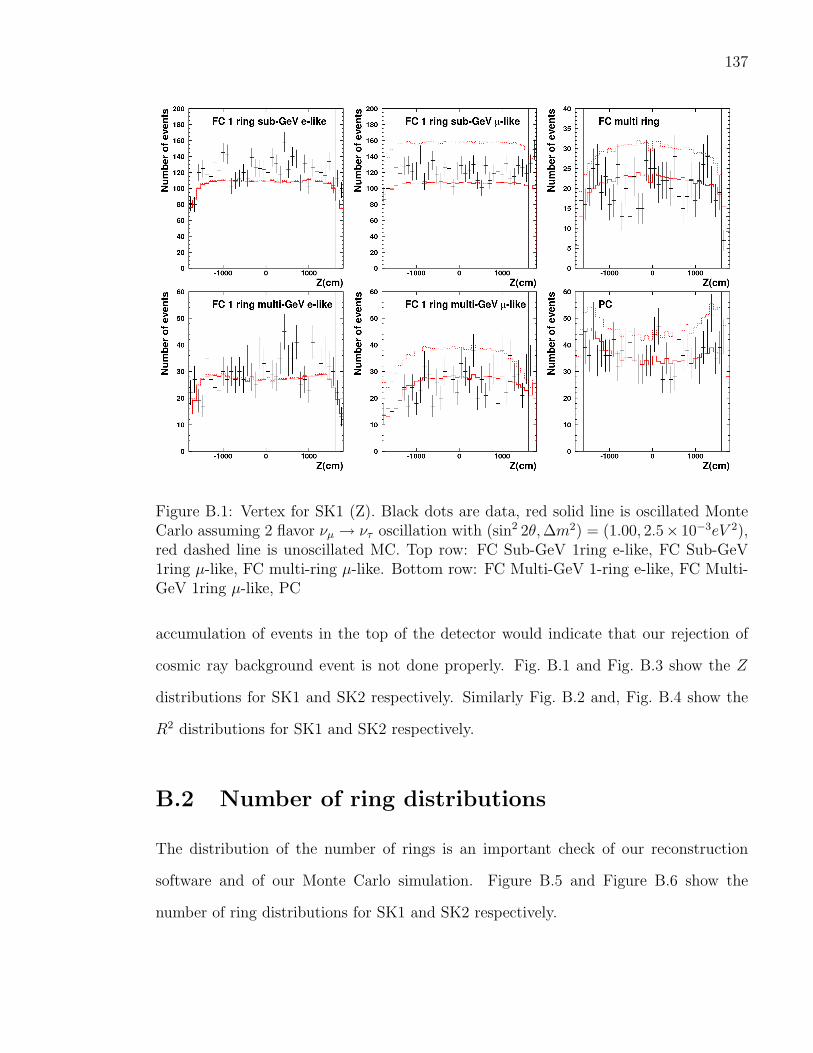
137
Figure B.1: Vertex for SK1 (Z). Black dots are data, red solid line is oscillated MonteCarlo assuming 2 flavor νµ → ντ oscillation with (sin2 2θ,∆m2) = (1.00, 2.5× 10⁻³eV 2),red dashed line is unoscillated MC. Top row: FC Sub-GeV 1ring e-like, FC Sub-GeV1ring µ-like, FC multi-ring µ-like. Bottom row: FC Multi-GeV 1-ring e-like, FC Multi-GeV 1ring µ-like, PC
accumulation of events in the top of the detector would indicate that our rejection of
cosmic ray background event is not done properly. Fig. B.1 and Fig. B.3 show the Z
distributions for SK1 and SK2 respectively. Similarly Fig. B.2 and, Fig. B.4 show the
R2 distributions for SK1 and SK2 respectively.
B.2 Number of ring distributions
The distribution of the number of rings is an important check of our reconstruction
software and of our Monte Carlo simulation. Figure B.5 and Figure B.6 show the
number of ring distributions for SK1 and SK2 respectively.

138
Figure B.2: Vertex for SK1 (R2). Black dots are data, red solid line is oscillated MonteCarlo assuming 2 flavor νµ → ντ oscillation with (sin2 2θ,∆m2) = (1.00, 2.5× 10⁻³eV 2),red dashed line is unoscillated MC. Top row: FC Sub-GeV 1ring e-like, FC Sub-GeV1ring µ-like, FC multi-ring µ-like. Bottom row: FC Multi-GeV 1-ring e-like, FC Multi-GeV 1ring µ-like, PC
B.3 PID distributions
Since the L/E analysis studies the oscillation of νµ into ντ , it is crucial to understand
our ability to distinguish muon-like events from electron-like events. Comparing the
distribution of the PID parameter for each sample is a check of our reconstruction
software and our Monte Carlo simulation. As you can see in Fig. B.7 and Fig. B.8,
the separation between e-like and µ-like events is very good for single-ring events. For
multi-ring events, it is more challenging. Most of PC events are CCνµ events so we do
not use the PID for PC events.

139
Figure B.3: Vertex for SK2 (Z). Black dots are data, red solid line is oscillated MonteCarlo assuming 2 flavor νµ → ντ oscillation with (sin2 2θ,∆m2) = (1.00, 2.5× 10⁻³eV 2),red dashed line is unoscillated MC. Top row: FC Sub-GeV 1ring e-like, FC Sub-GeV1ring µ-like, FC multi-ring µ-like. Bottom row: FC Multi-GeV 1-ring e-like, FC Multi-GeV 1ring µ-like, PC

140
Figure B.4: Vertex for SK2 (R2). Black dots are data, red solid line is oscillated MonteCarlo assuming 2 flavor νµ → ντ oscillation with (sin2 2θ,∆m2) = (1.00, 2.5× 10⁻³eV 2),red dashed line is unoscillated MC. Top row: FC Sub-GeV 1ring e-like, FC Sub-GeV1ring µ-like, FC multi-ring µ-like. Bottom row: FC Multi-GeV 1-ring e-like, FC Multi-GeV 1ring µ-like, PC

141
Figure B.5: Number of rings for SK1 . Black dots are data, red solid line is oscillatedMonte Carlo assuming 2 flavor νµ → ντ oscillation with (sin2 2θ,∆m2) = (1.00, 2.5 ×10⁻³eV 2), red dashed line is unoscillated MC. Top row: FC Sub-GeV 1ring e-like, FCSub-GeV 1ring µ-like, FC multi-ring µ-like. Bottom row: FC Multi-GeV 1-ring e-like,FC Multi-GeV 1ring µ-like, PC

142
Figure B.6: Number of rings for SK2 . Black dots are data, red solid line is oscillatedMonte Carlo assuming 2 flavor νµ → ντ oscillation with (sin2 2θ,∆m2) = (1.00, 2.5 ×10⁻³eV 2), red dashed line is unoscillated MC. Top row: FC Sub-GeV 1ring e-like, FCSub-GeV 1ring µ-like, FC multi-ring µ-like. Bottom row: FC Multi-GeV 1-ring e-like,FC Multi-GeV 1ring µ-like, PC

143
Figure B.7: PID likelihood for SK1 . Black dots are data, blue solid line is oscillatedMonte Carlo assuming 2 flavor νµ → ντ oscillation with (sin2 2θ,∆m2) = (1.00, 2.5 ×10⁻³eV 2), blue hatched are true CCνµ from oscillated MC, red dashed line is unoscillatedMC. Top left: FC single rine sub-GeV. Top right: FC single ring multi-GeV. Bottomleft: FC multi-ring, Bottom right: PC.

144
Figure B.8: PID likelihood for SK2 . Black dots are data, blue solid line is oscillatedMonte Carlo assuming 2 flavor νµ → ντ oscillation with (sin2 2θ,∆m2) = (1.00, 2.5 ×10⁻³eV 2), blue hatched are true CCνµ from oscillated MC, red dashed line is unoscillatedMC. Top left: FC single rine sub-GeV. Top right: FC single ring multi-GeV. Bottomleft: FC multi-ring, Bottom right: PC.

Appendix C
Proof that binned and unbinned
likelihood are equivalent
The goal of this Appendix is to show that using a binned or unbinned likelihood is
identical if the same binned MC is used.
In our L/E analysis we use a binned likelihood which can be written as a reduced χ2
(as in Eq. 9.2, Section 9.1):
χ2 =nbin∑i=1
[2(N exp
i (1+
nsys∑j=1
f ij ·εj)−N obsi )−2N obs
i ln( N obs
i
N expi (1 +
∑nsysj=1 f
ij · εj)
)]+
nsys∑j
(εj
σsysj
)2.
(C.1)
By assuming that the parameter εj are small, we can do a linear expansion of the χ2
as a function of εj and this leads to the following set of linear equations (as in Eq. 9.3,
where we kept only the linear terms):
nbin∑i=1
(N obsi −N
expi )f ik =
nsys∑j=1
(δjkσ2
+nbin∑i=1
N obsi f ijf
ik)εk. (C.2)
If instead of using a binned likelihood we wanted to use an unbinned likelihood, the
145

146
definition of lnL is the following:
lnL =
Nobs∑i
ln(N exp · P (xi|α))
−N exp
=
Nobs∑i
ln(Q(xi|α))
−N exp,
(C.3)
where Q is the non-normalized version of P . If our p.d.f P (and Q) are estimated using
Monte Carlo, they will be binned. And if the binning of the Monte Carlo is the same
as the binning that was applied to the data in the previous case then the following is
true. We first apply the pull terms method to the unbinned likelihood and we get that:
Qi = (1 +
nsys∑i=k
f ik · εk)Q0i . Then using the fact that the p.d.f Q is binned we can rewrite
N exp as follows:
N exp =nbin∑i=ibin
Qibin
=nbin∑i=ibin
(1 +
nsys∑i=k
f ibink · εk)Q0ibin.
(C.4)
So if we plug that back into Eq. C.3 and add the pull term −12
∑nsysk=1
ε2kσ2 , we get
lnL =[Nobs∑i=1
ln(1 +
nsys∑k=1
fki εk) + lnQ0i
]−
nbin∑bin=1
(1 +
nsys∑j=1
f binj εj)Q0bin (C.5)
− 1
2
nsys∑k=1
ε2kσ2, (C.6)

147
which leads to the following set of linear equations if we apply the same linear expansion
as before:
nobs∑i=1
f ik −nbin∑bin=1
fkbinQ0bin =
nsys∑j=1
(δjkσ2
+nobs∑i=1
f ijfik)εk. (C.7)
Now since Q0i = N exp
i and since you can write
nobs∑i=1
=nbin∑bin=1
nobs∑i=1
δi,bin =nbin∑bin=1
N obsbin , (C.8)
then the set of linear equation for the log likelihood becomes:
nbin∑bin=1
N obsbin f
bink −
nbin∑bin=1
f bink N expbin =
nsys∑k=1
(δjkσ2
+nbin∑bin=1
N obsbin f
binj f bink )εk, (C.9)
which is the same as the set of linear equations obtained with the binned data and
presented in Eq. C.2.

Appendix D
Use of a fully reconstructed charged
current quasi-elastic (CCQE)
sample
For quasi-elastic charged current interaction ν + n → p + e−, our accuracy on the
reconstruction of the energy and the flight length of the neutrino is limited by the fact
that in most cases we do not see the recoiling proton coming from a neutrino interaction.
If we were able to see the recoiling proton, our reconstruction of the energy and flight
length would be more accurate. In some cases, the recoil proton is above Cherenkov
threshold and if it is properly identified, we can collect a sample of events for which all
the kinematics variables are known. In that case, the energy and the flight length of the
incoming neutrino can be fully reconstructed. We call this sample the CCQE sample.
Events with one or two rings are used in the CCQE event search. The tools used to
identify the recoiling proton are based on Maxim Fechner’s work [76].
148

149
D.1 Selecting the CCQE sample
For two rings events, in 97% of cases, it was found that the first ring found is the lepton
and the second is the proton. We apply the following set of cuts to select the two-ring
CCQE sample:
• First, we select events inside the L/E fiducial volume, with 2 fully-contained rings
and with 100 < Evis < 4000 MeV.
• Then we use a cut designed to remove background from charged pions. By applying
a linear cut on the proton-like momentum (momentum computed assuming that
the particle is a proton) and track lengths: A < P < B×L(m)+C with A = C =
1.1 GeV and B = 7/6 GeV/c/m, we can remove charged pions which typically
have true momenta between 200 and 300 MeV/c and a proton-like momenta of
1.6 GeV/c, because their fitted path lengths are short (≈ 20 cm) due to pion
interactions.
• We then require that the opening angle of the second ring be less than 34 to select
particle with low β.
• Then, we use a specific pattern likelihood. We ask that
log(Llepton+proton)− log(Llepton+muon) be greater than zero.
• At this stage, there are still non-CCQE events coming from mis-identified pions.
To remove these, we apply a kinematic cut. We ask that the quantity V 2 (where
V = Pp + Pl − Pn) be around zero, since for a true CCQE event V is the 4-
momentum of the neutrino and V 2 is the invariant mass of the neutrino. Pp, Pl,
Pn are the 4-momenta of the proton, lepton and neutron respectively. We therefore
select events which peak at V 2 = 0 by asking −0.75 < V 2 < 1.5 GeV/c2.

150
Monte Carlo studies show that, for some events, the proton is missed by the standard
fitter even if it is above Cherenkov threshold. These events only have one ring corre-
sponding to the lepton track. We found that in these cases, the proton ring is weak
but visible by eye-scan, and a dedicated ring finding algorithm was developed to find
such events. Using this new ring algorithm and the pattern likelihood, we can build
the estimator ∆L to decide whether an event is a true single-ring event, or if a proton
above Cherenkov threshold was missed (∆L = log[log(Llepton+proton)− log(Llepton alone)]).
A high value of the estimator corresponds to a proton track. To select the single-ring
CCQE sample, we apply the following cuts:
• First, we select events inside the L/E fiducial volume, with 1 fully-contained ring
and with 100 < Evis < 4000 MeV.
• Using the output of the proton pattern fitter on the new ring candidate, we apply
A < P < B ×L(m) +C with A = C = 1.1 GeV and B = 7/6 GeV/c/m. We also
require that the track length L be greater than 2 m.
• The estimator Qdens is based on the light distribution along the edge of a ring. It
is used to decide if a ring was well fitter or not. We ask logQdens > 0 to select
good ring candidates.
• We ask that the ∆L pattern ID estimator be larger than 3.
• Finally, we ask that the V 2 quantity defined above be larger than 0.75 GeV/c2.
D.2 Energy and flight length reconstruction for the
CCQE sample
Once the selection of the CCQE sample is completed, we can fully reconstruct the
energy and flight length using the kinematics of the interaction. We can then test if

151
this fully reconstructed energy and flight length are more accurate than the standard
reconstruction. In Fig. D.1 we present the reconstruction of the energy and the flight
length and in Fig. D.2 we present the resulting L/E reconstruction. We can see that
the energy of the single-ring events is usually reconstructed too low with the standard
tools, as expected from missing the proton, and that this is very much improved when
using the full CCQE reconstruction. The flight length reconstruction is also significantly
improved by using the full kinematic reconstruction.
D.3 Statistics of the CCQE sample
We tested the use of the CCQE sample only on 100 years of SK1 MC. In Table D.1
we present the events that are identified as CCQE events and can be used in the L/E
analysis. Out of the events that are found to be CCQE and inside the fiducial volumed
defined for the L/E analysis and after we applied an energy cut on the 2-rings sample,
if we select µ-like events, we expect 41 events in the 1-ring sample and 12 events in the
2-rings sample. For the 1-ring sample, out of the 41 events, 20 were passing the L/E
resolution cut and were already included in the L/E analysis but with a worse energy
and flight length reconstruction. The 21 other events are events that were not used
before as they were failing the resolution cut. They can now be added since the energy
and flight length resolution of the CCQE sample is much better. The same is true for
the 2-rings sample, and 7 events are expected to be added. At this point it is important
to notice that the identified CCQE sample account for only 2% of all L/E events, and
therefore the effect of using this sample is expected to be very small, if even visible.

152
1-ring 2-rings
Energy (GeV)
Flight Length (km)
Figure D.1: Reconstructed versus true energy (top) and flight length (bottom) forevents identified as CCQE and passing the L/E resolution cut. Black circles are eventsreconstructed with the CCQE full kinematics, while red triangles are the same eventsreconstructed with the standard L/E tools. The first column is for the 1-ring sample,while the second column is for the 2-rings sample.

153
1-ring 2-rings
L/E bins
Resolution
Figure D.2: The top row is the reconstructed L/E bin versus the true L/E bin forevents identified as CCQE and passing the L/E resolution cut. Black circles are eventsreconstructed with the CCQE full kinematics, while red triangles are the same eventsreconstructed with the standard L/E tools. The first column is for the 1-ring sample,while the second column is for the 2-rings sample. The bottom row is the true L/E binminus the reconstructed L/E bin for the CCQE reconstruction (black) and the standardreconstruction (red).

154
1-ring sample (MC) 2-rings sample (MC)CCQE (FV for L/E) 58.99 52.67evis > 600 21.92µ-like 41.10 12.44resolution cut < 0.7 19.68 6.61total L/E events 2084.55 634.17
Table D.1: CCQE sample statistics, MC is normalized to 1489 days of livetime, and isnot oscillated.
D.4 Testing the sensitivity of the CCQE sample
In order to test if adding the CCQE sample to the L/E analysis is useful, we compute
a sensitivity curve for the regular L/E analysis and the L/E analysis with the CCQE
sample. To compute the sensitivity curve, we create a set of fake data which agrees
perfectly with an oscillated Monte Carlo and with the SK1 livetime. Such a set can be
seen in Fig. D.3.
Then we apply the χ2 fit to this set of fake data. Of course the value of the best
fit χ2 will be very low, but the contours represent the sensitivity achievable by the
analysis. We applied this method to both the standard L/E analysis and the CCQE
L/E analysis, where the events identified as CCQE have been reconstructed using the
full kinematics of the interaction and for which the resolution cut was not applied. As
you can see in Fig. D.4, the sensitivity of the CCQE L/E analysis is not distinguishable
from the contours obtained with the standard L/E analysis. It was therefore decided
not to add the CCQE sample to the L/E analysis.

155
Figure D.3: Example of fake dataset (black dots) which agree perfectly with the os-cillated Monte Carlo (red solid line). The unoscillated MC is also shown (black solidline).
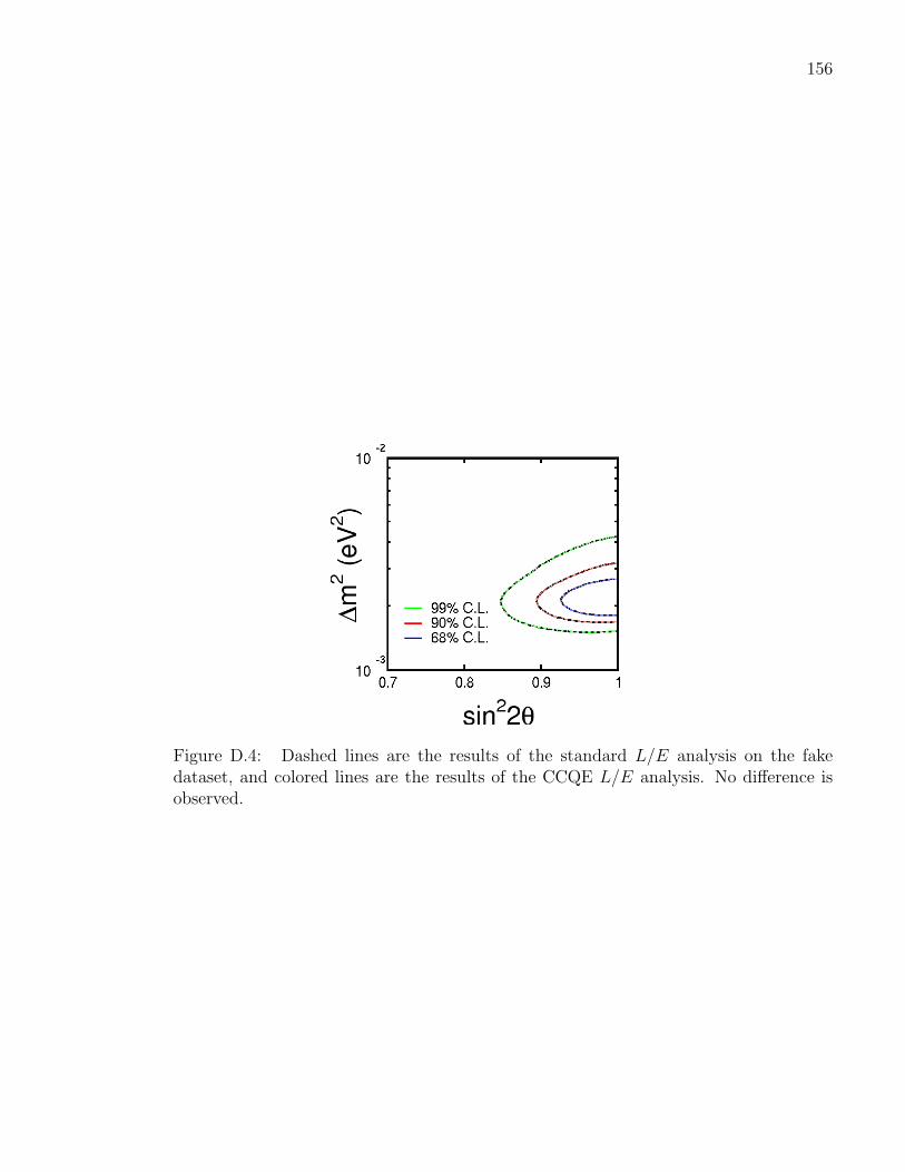
156
Figure D.4: Dashed lines are the results of the standard L/E analysis on the fakedataset, and colored lines are the results of the CCQE L/E analysis. No difference isobserved.

157
List of Journal Abbreviation
Ann. Phys. . . . . . . . . . . . . . . . . . . . . . . . . . . . . . . . . . . . . . . . . . . . . . . . . . . . . . . . . Annals of Physics
AIP Conf. Proc . . . . . . . . . . . . . . . .American Institute of Physics Conference Proceedings
Astropart. Phys . . . . . . . . . . . . . . . . . . . . . . . . . . . . . . . . . . . . . . . . . . . . . . . . Astroparticle Physics
Astrophys. J. . . . . . . . . . . . . . . . . . . . . . . . . . . . . . . . . . . . . . . . . . . . . . . . . . . Astrophysical Journal
CERN . . . . . . . . . . . . . . . . . . . . . . . . . . . . . . . . . . Conseil Europeen pour la recherche nucleaire
Eur. Phys. J. . . . . . . . . . . . . . . . . . . . . . . . . . . . . . . . . . . . . . . . . . . . . . European Physical Journal
JHEP . . . . . . . . . . . . . . . . . . . . . . . . . . . . . . . . . . . . . . . . . . . . . . . . Journal of High Energy Physics
Los Alamos Sci. . . . . . . . . . . . . . . . . . . . . . . . . . . . . . . . . . . . . . . . . . . . . . . . . Los Alamos Scientific
New J. Phys. . . . . . . . . . . . . . . . . . . . . . . . . . . . . . . . . . . . . . . . . . . . . . . . . .New Journal of Physics
Nucl. Instrum. Meth. . . . . . . . . . . . . . . . . . . . . . . . . . . . . . Nuclear Instruments and Methods
Nucl. Phys. . . . . . . . . . . . . . . . . . . . . . . . . . . . . . . . . . . . . . . . . . . . . . . . . . . . . . . . . . Nuclear Physics
Nucl. Phys. Proc. Suppl . . . . . . . . . . . . . . . . . . Nuceal Physics - Proceedings Supplements
Phys. Rept . . . . . . . . . . . . . . . . . . . . . . . . . . . . . . . . . . . . . . . . . . . . . . . . . . . . . . . . . . Physics Reports
Phys. Rev. . . . . . . . . . . . . . . . . . . . . . . . . . . . . . . . . . . . . . . . . . . . . . . . . . . . . . . . . . . Physical Review
Phys. Rev. Lett. . . . . . . . . . . . . . . . . . . . . . . . . . . . . . . . . . . . . . . . . . . . . Physical Review Letters
Prog. Theor. Phys . . . . . . . . . . . . . . . . . . . . . . . . . . . . . . . . . . . Progress of Theoretical Physics
Rev. Mod. Phys . . . . . . . . . . . . . . . . . . . . . . . . . . . . . . . . . . . . . . . . . . Review of Modern Physics
Sov. Phys. JETP . . . Soviet Physics, Journal of Experimental and Theoretical Physics
World Sci. Lect. Notes Phys. . . . . . . . . . . . . . . World Scientific Lectures Notes in Physics

Bibliography
[1] Super-Kamiokande, Y. Ashie et al., hep-ex/0501064.
[2] Z. Maki, M. Nakagawa, and S. Sakata, Prog. Theor. Phys. 28, 870 (1962).
[3] B. Pontecorvo, Sov. Phys. JETP 26, 984 (1968).
[4] T. Schwetz, M. Tortola, and J. W. F. Valle, New J. Phys. 10, 113011 (2008),
0808.2016.
[5] Y. Fukuda et al., Nucl. Instrum. Meth. A501, 418 (2003).
[6] G. Mituska, Study of non-standard neutrinos interactions with atmospheric neu-
trino data in Super-Kamiokande, PhD thesis, University of Tokyo, 2009.
[7] W. Pauli, Letter to the physical society of tubingen (1930), reproduced in physics
today, 31,(9):23, 1978.
[8] F. Reines and C. L. Cowan, Phys. Rev. 90, 492 (1953).
[9] G. Danby et al., Phys. Rev. Lett. 9, 36 (1962).
[10] DONUT, K. Kodama et al., Phys. Lett. B 204, 218 (2001), hep-ex/0012035.
[11] B. T. Cleveland et al., Astrophys. J. 496, 505 (1998).
[12] J. N. Bahcall and R. K. Ulrich, Rev. Mod. Phys. 60, 297 (1988).
158

159
[13] Kamiokande-II, K. S. Hirata et al., Phys. Lett. B 280, 146 (1992).
[14] R. Becker-Szendy et al., Nucl. Phys. Proc. Suppl. 38, 331 (1995).
[15] F. Halzen and A. D. Martin, Quarks and leptons: an introductory course in modern
particle physics .
[16] S. L. Glashow, in Quarks and Leptons, Cargese 1979, p. 707, 1980.
[17] M. Gell-Mann, P. Ramond, and R. Slansky, Supergravity (, 1979).
[18] R. N. Mohapatra and G. Senjanovic, Phys. Rev. Lett. 44, 912 (1980).
[19] T. Yanagida, Horizontal symmetry and masses of neutrinos, in Proceedings of the
Workshop on Unified Theory and the Baryon Number of the Universe, p. 95, KEK,
Japan, 1979.
[20] B. Kayser, F. Gibrat-Debu, and F. Perrier, World Sci. Lect. Notes Phys. 25, 1
(1989).
[21] R. Slansky, S. Raby, J. T. Goldman, and G. Garvey, Los Alamos Sci. 25, 28 (1997).
[22] N. Cabibbo, Phys. Rev. Lett. 10, 531 (1963).
[23] M. Kobayashi and T. Maskawa, Progress of Theoretical Physics 49, 652 (1973).
[24] F. Boehm and P. Vogel, Physics of Massive Neutrinos (Cambridge University Press,
1992).
[25] A. G. Cohen, S. L. Glashow, and Z. Ligeti, (2008), arXiv 0810.4602.
[26] R. N. Mohapatra and W. Rodejohann, Phys. Rev. D72, 053001 (2005), hep-
ph/0507312.
[27] MINOS, P. Adamson et al., Phys. Rev. Lett. 101, 131802 (2008), 0806.2237.

160
[28] CHOOZ, M. Apollonio et al., Phys. Lett. B466, 415 (1999), hep-ex/9907037.
[29] T2K, Y. Itow et al., (2001), hep-ex/0106019.
[30] Double Chooz, F. Ardellier et al., (2006), hep-ex/0606025.
[31] M. Ishitsuka, T. Kajita, H. Minakata, and H. Nunokawa, Phys. Rev. D72, 033003
(2005), hep-ph/0504026.
[32] V. Barger et al., Phys. Rev. D74, 073004 (2006), hep-ph/0607177.
[33] J. E. Campagne, M. Maltoni, M. Mezzetto, and T. Schwetz, JHEP 04, 003 (2007),
hep-ph/0603172.
[34] LSND, A. Aguilar et al., Phys. Rev. D64, 112007 (2001), hep-ex/0104049.
[35] MiniBooNE, A. A. Aguilar-Arevalo et al., Phys. Rev. Lett. 100, 032301 (2008),
0706.0926.
[36] Super-Kamiokande, S. Fukuda et al., Phys. Rev. Lett. 86, 5656 (2001), hep-
ex/0103033.
[37] SNO, Q. R. Ahmad et al., Phys. Rev. Lett. 89, 011301 (2002), nucl-ex/0204008.
[38] Borexino, C. Arpesella et al., Phys. Lett. B658, 101 (2008), 0708.2251.
[39] KamLAND, S. Abe et al., Phys. Rev. Lett. 100, 221803 (2008), 0801.4589.
[40] K2K, E. Aliu et al., Phys. Rev. Lett. 94, 081802 (2005), hep-ex/0411038.
[41] R. Claus et al., Nucl. Instrum. Meth. A261, 540 (1987).
[42] R. Becker-Szendy et al., Nucl. Instrum. Meth. A324, 363 (1993).
[43] Hamamatsu website http://www.hamamatsu.com/.

161
[44] M. Honda, T. Kajita, K. Kasahara, S. Midorikawa, and T. Sanuki, Phys. Rev.
D75, 043006 (2007), astro-ph/0611418.
[45] G. Battistoni, A. Ferrari, T. Montaruli, and P. R. Sala, Astropart. Phys. 19, 269
(2003), hep-ph/0207035.
[46] G. D. Barr, T. K. Gaisser, P. Lipari, S. Robbins, and T. Stanev, Phys. Rev. D70,
023006 (2004), astro-ph/0403630.
[47] M. Ishitsuka, L/E analysis of the atmospheric neutrino data from Super-
Kamiokande, PhD thesis, University of Tokyo, 2004.
[48] Y. Hayato, Nucl. Phys. Proc. Suppl. 112, 171 (2002).
[49] G. Mitsuka, AIP Conf. Proc. 981, 262 (2008).
[50] G. Mitsuka, AIP Conf. Proc. 967, 208 (2007).
[51] C. H. Llewellyn Smith, Phys. Rept. 3, 261 (1972).
[52] R. A. Smith and E. J. Moniz, Nucl. Phys. B43, 605 (1972).
[53] D. H. Perkins, Introduction to high energy physics , Reading 1972, 353p.
[54] K2K, R. Gran et al., Phys. Rev. D74, 052002 (2006), hep-ex/0603034.
[55] X. Espinal and F. Sanchez, AIP Conf. Proc. 967, 117 (2007).
[56] J. Reich et al., Nucl. Instrum. Meth. A440, 535 (2000).
[57] D. Rein and L. M. Sehgal, Ann. Phys. 133, 79 (1981).
[58] M. Gluck, E. Reya, and A. Vogt, Eur. Phys. J. C5, 461 (1998), hep-ph/9806404.
[59] A. Bodek and U. K. Yang, (2003), hep-ex/0308007.
[60] T. Sjostrand, CERN-TH-7112-93.

162
[61] D. Rein and L. M. Sehgal, Nucl. Phys. B223, 29 (1983).
[62] K2K, M. Hasegawa et al., Phys. Rev. Lett. 95, 252301 (2005), hep-ex/0506008.
[63] D. Rein and L. M. Sehgal, Phys. Lett. B657, 207 (2007), hep-ph/0606185.
[64] Geant detector description and simulation tool, 1993, CERN Program Library
Long Writeup W5013.
[65] C. Zeitnitz and T. A. Gabriel, Nucl. Instrum. Meth. A349, 106 (1994).
[66] Y. Takenaga, Atmospheric neutrino oscillation analysis with solar terms in Super-
Kamiokande, PhD thesis, University of Tokyo, 2008.
[67] W. Wang, Study of non-standard effects in neutrino oscillations at Super-
Kamiokande, PhD thesis, Boston University, 2007.
[68] E. R. Davies, Machine Vision: Theory, Algorithms, Practicalities (Morgan Kauf-
mann Publishers Inc., San Francisco, CA, USA, 2004).
[69] S. T. Clark, Searches for proton decay with the Super-Kamiokande detector, PhD
thesis, Boston University, 2007.
[70] Soudan 2, M. C. Sanchez et al., Phys. Rev. D68, 113004 (2003), hep-ex/0307069.
[71] V. D. Barger, J. G. Learned, S. Pakvasa, and T. J. Weiler, Phys. Rev. Lett. 82,
2640 (1999), astro-ph/9810121.
[72] D. A. Krakauer et al., Phys. Rev. D44, 6 (1991).
[73] E. Lisi, A. Marrone, and D. Montanino, Phys. Rev. Lett. 85, 1166 (2000), hep-
ph/0002053.
[74] G. L. Fogli, E. Lisi, A. Marrone, D. Montanino, and A. Palazzo, Phys. Rev. D66,
053010 (2002), hep-ph/0206162.

163
[75] Particle Data Group, R. M. Barnett et al., Phys. Rev. D54, 1 (1996).
[76] Super-Kamiokande, M. Fechner et al., (2009), arXiv 0901.1645.

Curriculum Vitae
Fanny Dufour
590 Commonwealth Avenue Mobile: + 1-617-888-0075
Department of Physics, Boston University Office: + 1-617-353-6040
Boston, MA 02215, U.S.A. E-mail: [email protected]
EDUCATION
• Boston University, Boston, U.S.A.
– Ph.D. in Physics, expected in May 2009
• Universite Libre de Bruxelles, Brussels, Belgium
– Bachelor of Science in Physics, June 2003, La plus grande Distinction
RESEARCH EXPERIENCE
• Super-Kamiokande
– Detector hardware work: Installation of outer detector reflector
– Monte Carlo work: tuning of the outer detector simulation; generation of 60
years of Nuance MC
– Data processing: reduction of partially contained neutrino events and studies
of associated systematic uncertainties
– Physics analysis: L/E oscillation analysis
• T2KK and Long baseline neutrino experiments
164

165
– Physics analysis: Likelihood study to remove neutral pion background events
from electron neutrino appearance signal; Study of off-axis sensitivity of the
Korean detector in the T2KK framework
– Physics analysis: Comparison of the T2KK setup and the FNAL wide-band
beam proposal, using the same analysis framework.
PRESENTATIONS
• Sensitivity of the JPARC-Kamioka-Korea setup with 2 Water Cerenkov
detectors
CHIPP 2008
Zurich, Switzerland, Nov 17 - 18, 2008
• T2KK
NOW 2008
Lecce, Italy, Sept 6 - 13, 2008
• CP Violation Physics at a J-PARC Beam - Water Cherenkov Detector
Case
NP08
Mito, Japan, March 5 - 7, 2008
• Wide-band beam studies for T2KK
3rd International Workshop on a Far Detector in Korea for the J-PARC Neutrino
Beam
Tokyo University, Tokyo, Japan, Sept 30 - Oct 1, 2007
• T2KK and Examination of Water Detector Capability
FNAL/BNL joint study group for long baseline neutrino experiments,
Fermilab, U.S.A., September 16 - 17, 2006

166
• T2KK sensitivity as a function of off-axis angle
2nd International Workshop on a Far Detector in Korea for the J-PARC Neutrino
Beam
Seoul National University, Seoul, Korea, July 13 - 14, 2006
• Signal and background separation with 20 and 40% photo coverage of
a large Cherenkov detector
2nd International Workshop on a Far Detector in Korea for the J-PARC Neutrino
Beam
Seoul National University, Seoul, Korea, July 13 - 14, 2006
SELECTED PUBLICATIONS
• Study of the T2KK setup with several off-axis angles of the Korean
detector and new systematic errors
F. Dufour, T. Kajita, E. Kearns and K. Okumura
In preparation
• Report of the US long baseline neutrino experiment study
V. Barger et al.
arXiv:0705.4396 [hep-ph].
OTHER PUBLICATIONS
as a member of the Super-Kamiokande collaboration
• Solar neutrino measurements in Super-Kamiokande-II
J. P. Cravens et al.
Phys. Rev. D 78, 032002 (2008)
arXiv:0803.4312 [hep-ex]
• Search for Matter-Dependent Atmospheric Neutrino Oscillations in Super-
Kamiokande

167
K. Abe et al.
Phys. Rev. D 77, 052001 (2008)
arXiv:0801.0776 [hep-ex]
• Study of TeV Neutrinos with Upward Showering Muons in Super-
Kamiokande
S. Desai et al.
Astropart. Phys. 29, 42 (2008)
arXiv:0711.0053 [hep-ex]
• Search for Supernova Neutrino Bursts at Super-Kamiokande
M. Ikeda et al.
Astrophys. J. 669, 519 (2007)
arXiv:0706.2283 [astro-ph]
• Search for neutral Q-balls in Super-Kamiokande II
Y. Takenaga et al.
Phys. Lett. B 647, 18 (2007)
arXiv:hep-ex/0608057
• A measurement of atmospheric neutrino flux consistent with tau neu-
trino appearance
K. Abe et al.
Phys. Rev. Lett. 97, 171801 (2006)
arXiv:hep-ex/0607059
• Search for diffuse astrophysical neutrino flux using ultra-high energy
upward-going muons in Super-Kamiokande I
M. E. C. Swanson et al.

168
Astrophys. J. 652, 206 (2006)
arXiv:astro-ph/0606126
TEACHING EXPERIENCE
• Boston University, Boston, U.S.A.
– Discussion session tutor of college physics, September 2003 – June 2004
• Universite Libre de Bruxelles, Brussels, Belgium
– Office hours teaching assistant physics, September 2002 – December 2002
HONORS AND AWARDS
• Gertrude and Maurice Goldhaber Prize, Boston University, Boston, U.S.A.,
2005
• BAEF fellowship for Belgian Graduate Students in the U.S.A., Brussels, Bel-
gium, 2003
ORGANIZATIONS
• Member of the Physics Graduate Students Committee of Boston University, 2005-
2009
• Founding member of the Women in Physics association at Boston University, 2006-
2009
REFERENCES
• Professor Edward Kearns
Department of Physics, Boston University
E-mail: [email protected]; Office Phone: + 1-617-353-3425

169
• Professor Kate Scholberg
Department of Physics, Duke University
E-mail: [email protected] ; Office Phone: + 1-919-660-2962
• Professor Takaaki Kajita
Institute for Cosmic Ray Research, University of Tokyo
E-mail: [email protected] ; Office Phone: + 81-4-7136-3100