This is a repository copy of Probing quantum decoherence in atmospheric neutrino oscillations with a neutrino telescope.

White Rose Research Online URL for this paper:http://eprints.whiterose.ac.uk/102563/

Version: Accepted Version

Article:

Morgan, D., Winstanley, E. orcid.org/0000-0001-8964-8142, Brunner, J. et al. (1 more author) (2006) Probing quantum decoherence in atmospheric neutrino oscillations with a neutrino telescope. Astroparticle Physics, 25 (5). pp. 311-327. ISSN 0927-6505

https://doi.org/10.1016/j.astropartphys.2006.03.001

Article available under the terms of the CC-BY-NC-ND licence (https://creativecommons.org/licenses/by-nc-nd/4.0/)

eprints@whiterose.ac.ukhttps://eprints.whiterose.ac.uk/

Reuse

This article is distributed under the terms of the Creative Commons Attribution-NonCommercial-NoDerivs (CC BY-NC-ND) licence. This licence only allows you to download this work and share it with others as long as you credit the authors, but you can’t change the article in any way or use it commercially. More information and the full terms of the licence here: https://creativecommons.org/licenses/

Takedown

If you consider content in White Rose Research Online to be in breach of UK law, please notify us by emailing eprints@whiterose.ac.uk including the URL of the record and the reason for the withdrawal request.

arX

iv:a

stro

-ph/

0412

618v

2 2

8 M

ay 2

006

Probing Quantum Decoherence in

Atmospheric Neutrino Oscillations with a

Neutrino Telescope

Dean Morgan a Elizabeth Winstanley a,∗ Jurgen Brunner b

Lee F. Thompson c

aDepartment of Applied Mathematics, The University of Sheffield, Hicks Building,

Hounsfield Road, Sheffield, S3 7RH, U.K.

bCentre de Physique des Particules de Marseille, 163 Avenue de Luminy -

Case 907, 13288 Marseille Cedex 09, France.

cDepartment of Physics and Astronomy, The University of Sheffield,

Hicks Building, Hounsfield Road, Sheffield, S3 7RH, U.K.

Abstract

Quantum decoherence, the evolution of pure states into mixed states, may be afeature of quantum gravity. In this paper, we show how these effects can be modelledfor atmospheric neutrinos and illustrate how the standard oscillation picture ismodified. We examine how neutrino telescopes, such as ANTARES, are able toplace upper bounds on these quantum decoherence effects.

Key words: quantum decoherence, neutrino telescopesPACS: 03.65.Yz, 04.60.-m, 14.60.Pq, 14.60.St, 95.55.Vj, 96.40.Tv

1 Introduction

Quantum field theory and general relativity are supremely successful theo-ries, both having been experimentally verified to great accuracy. However,these two theories are fundamentally incompatible: general relativity is non-renormalizable as a quantum field theory. Many candidate theories of quantumgravity exist in the literature, but there is as yet no consensus as to whichwill provide the final fundamental theory. For a recent review of the current

∗ Corresponding authorEmail address: E.Winstanley@sheffield.ac.uk (Elizabeth Winstanley).

Preprint submitted to Astroparticle Physics 2 February 2008

state of play, see [1]. Quantum gravity becomes particularly important in tworealms of physics: the very early universe (prior to the Planck time, 10−43 s);and in black holes, when gravitational fields are strong but quantum effectscannot be ignored.

There are two different approaches to uncovering the theory of quantum grav-ity: firstly, there is the ‘top down’ method, which involves writing a theorydown and then attempting to see if the theory can make any physical predic-tions which are testable. The second, which is the method embraced here, isthe ‘bottom up’ method, in which we analyze experimental data and attemptto fit the data to various phenomenological models (for a recent review, see,for example, [2]). This way, we may narrow down the number of models until,eventually, a single theory emerges, which is consistent with experiment. Thereare various ways in which quantum gravity may alter fundamental physics; thefinal theory will no doubt include highly unexpected effects on basic physicalprinciples. Here we are concerned only with one such mechanism: the influenceof quantum gravity on standard quantum mechanical time-evolution.

Naively, one might expect that quantum gravity is beyond the reach of ex-perimental physics, since its relevant energy scale is the Planck energy, ap-proximately 1019 GeV. However, recent theoretical models coming from stringtheory suggest that the energy scale of quantum gravity may be as low as afew TeV [3]. Moreover, even with more conservative estimates of the quan-tum gravity energy scale, comparatively low energy physics may be sensitiveto quantum gravity effects, for example, through quantum-gravity inducedmodifications of quantum mechanics resulting in quantum decoherence [4].

In this article we are concerned with one such low-energy system: atmosphericneutrinos. This is a comparatively simple quantum system, which lends it-self to an analysis of quantum decoherence effects. There is already a bodyof work on the theoretical modelling of quantum decoherence effects on neu-trino oscillations [5,6,7,8,9]. However, the only analysis of decoherence effectsin experimental data relating to νµ → ντ oscillations available in the literatureto date is for Super-Kamiokande and K2K data [10,11,12]. An initial analy-sis [10] was able to put bounds on quantum decoherence effects in a simplemodel. Subsequently, a detailed analysis of the same simple model [11] foundthat quantum decoherence effects were slightly disfavoured compared with thestandard oscillation scenario, but that they could not be completely ruled out.Further experimental work is therefore needed, and here we shall study thesensitivity of the ANTARES neutrino telescope [13] to these quantum decoher-ence effects in atmospheric neutrino oscillations. Although neutrino telescopessuch as ANTARES are primarily designed for the detection and study of neu-trinos of astrophysical and cosmological origin, atmospheric neutrinos formthe most important background to such sources and are likely to provide thefirst physics results.

2

As well as the simple model considered in Refs. [10,11], in this paper we shallstudy models which are more exotic than those considered previously, as theyinclude effects such as non-conservation of energy (within the neutrino sys-tem). Furthermore, while these models have been studied theoretically in theliterature [5,6,7,8,9], they have not been experimentally tested. It should beemphasized that such quantum decoherence is not the only possible effectof quantum gravity on neutrinos [14]. For example, quantum gravity is ex-pected to change the energy dependence of the oscillation length [15], andalso alter the dispersion relation [16], leading to observable effects [17]. Weshall also briefly discuss other, non-quantum gravity, possible corrections toatmospheric neutrino oscillations and how they relate to our models here, aswell as comparing our results on quantum decoherence parameters with thosecoming from other experimental (i.e. non-neutrino) systems (see, for example,[18,19]). Finally, although our simulations are specific to ANTARES, we an-ticipate that other high energy neutrino experiments such as AMANDA [20],IceCube [21] and NESTOR [22], may well be able to probe these effects.

Given the high energy and long path-length of atmospheric neutrinos stud-ied by ANTARES, this study is complementary to “long-baseline” neutrinooscillation experiments. As well as the analysis of K2K data [11], a relatedanalysis of KAMLAND data has also been performed in [23]. In both casesdecoherence is disfavoured over the standard oscillation picture. The potentialfor bounding quantum decoherence and other damping signatures in future re-actor experiments, such as MINOS [24] and OPERA [25], is discussed in [26].

The outline of this paper is as follows. In section 2, we discuss how quantumgravity may be expected to modify quantum mechanics, before applying theformalism developed to atmospheric neutrino oscillations in section 3. Westudy in detail some specific models of quantum decoherence in section 4, anddescribe the results of ANTARES sensitivity simulations for these models insection 5. The projected ANTARES sensitivities are compared with resultsfrom other experiments (both neutrino and non-neutrino) in section 6, and webriefly discuss other possible corrections to atmospheric neutrino oscillations insection 7. Finally, our conclusions are presented in section 8. Unless otherwisestated, we use units in which c = ~ = 1.

2 Quantum gravity induced modifications of quantum mechanics

In quantum gravity, space-time is expected to adopt a ‘foamy’ structure [27]:tiny black holes form out of the vacuum (in the same way that quantumparticles can be formed out of the vacuum). These will be very short-lived,evaporating quickly by Hawking radiation [28]. Each microscopic black holemay induce variations in the standard time-evolution of quantum mechanics,

3

as an initially pure quantum state (describing the space-time before the for-mation of the black hole) can evolve to a mixed quantum state (describing theHawking radiation left after the black hole has evaporated). In particular, inquantum gravity it is no longer necessarily the case that pure states cannotevolve to mixed states.

In order to describe this process, Hawking suggested a quantum gravitationalmodification of quantum mechanics [29], which is based on the density matrixformalism. An initial quantum state is described by a density matrix ρin, andthis state then evolves to a final state described by a density matrix ρout. Thetwo density matrices are related by

ρout = $ρin,

where $ is an operator known as the super-scattering operator. In ordinaryquantum mechanics, the super-scattering operator can be factorized as

$ = SS†, (1)

where S is the usual S-matrix. In this case, a pure initial state always leadsto a pure final state. However, in quantum gravity it is no longer necessarilythe case that the super-scattering matrix can be factorized as in equation(1), and, if it cannot, then the evolution from pure state to mixed state isallowed. The disadvantage of this approach is that it requires the constructionof asymptotic “in” and “out” states.

Therefore, here we will take an alternative approach, which is more useful forour application to atmospheric neutrino oscillations, allowing the evolutionof pure to mixed states by modifying the differential equation describing thetime-evolution of the density matrix ρ [4]. In standard quantum mechanicsthis differential equation takes the form

ρ = −i[H, ρ],

and could be modified by quantum gravity to the equation [4]

ρ = −i[H, ρ] + δ/Hρ. (2)

In the above equations, H is the Hamiltonian of the system, δ/H is the mostgeneral linear extension which maps hermitian matrices to hermitian matricesand the dot denotes differentiation with respect to time. Various conditionsneed to be imposed on δ/H to ensure that probability is still conserved and thatTrρ2 is never greater than unity [4]. These conditions will be implemented inthe next section when we apply this approach to atmospheric neutrinos. How-ever, the precise form of δ/H would need to come from a complete, final, theoryof quantum gravity. In this paper we take a phenomenological approach, mod-elling δ/H in a manner independent of its origin in quantum gravity. Ultimately

4

one may hope that experimental observations may be able to constrain theform of δ/H and hence its theoretical origin.

One form of δ/H which is frequently employed in the literature is the Lindbladform [30]

δ/Hρ =∑

n

[Dn, [Dn, ρ]] , (3)

where the Dn are self-adjoint operators which commute with the Hamiltonianof the theory. Such modifications of standard quantum-mechanical time evolu-tion have been widely studied, both as a solution to the quantum measurementproblem [31] and for decoherence due to the interaction with an environment[32]. In recent work in discrete quantum gravity, it has been shown that δ/Hhas the Lindblad form with a single operator D which is proportional to theHamiltonian H [33]. However, it should be emphasized that this is not theonly possible approach to quantum gravity, and that other formulations indi-cate that in general δ/H does not have the Lindblad form. This is the reasonfor our more general set-up in this paper.

Modifications of quantum mechanics (whether from quantum gravity or otherorigins) of the form (2) are often known as quantum decoherence effects as theyemerge from dissipative interactions with an environment (of which space-time foam is just one example), and allow transitions from pure to mixedquantum states (i.e. a loss of coherence). Such effects have been studied inquantum systems other than atmospheric neutrinos, for example, the neutralkaon system, for which there exists an extensive literature (see, for example,[18,19]).

It should be stressed that although our primary motivation for studying quan-tum decoherence is from quantum gravity, in fact our modelling in the sub-sequent sections is independent of the source of the quantum decoherence.Furthermore, Ohlsson [34] has discussed how Gaussian uncertainties in theneutrino energy and path length, when averaged over, can lead to modifica-tions of the standard neutrino oscillation probability which are similar in formto those coming from quantum decoherence, and which are therefore includedin our analysis. See also [35] for further discussion of these effects.

3 Quantum decoherence modifications of atmospheric neutrino os-

cillations

We now consider how quantum gravity induced modifications of quantum me-chanics, as outlined in the previous section, may affect atmospheric neutrinooscillations. The quantum system of interest is then simply made up of muonand tau neutrinos. The mathematical modelling of quantum decoherence ef-

5

fects in this system is not dissimilar to that for the neutral kaon system [4,18].In this paper we will assume that quantum decoherece affects neutrinos andanti-neutrinos in the same way, and do not consider the possibility that quan-tum decoherence may appear only in the anti-neutrino sector [36].

In order to implement equation (2) for the system of atmospheric muon andtau neutrinos, we need to represent the matrices H and ρ in terms of a specificbasis which comprises the standard Pauli matrices σi. We may, therefore, writethe density matrix, Hamiltonian and additional term δ/H in terms of the Paulimatrices as

ρ =1

2ρµσµ; H =

1

2hνσν ; δ/H =

1

2h′

κσκ;

where the Greek indices run from 0 to 3, and a summation over repeatedindices is understood. Similarly decomposing the time derivative of the densitymatrix,

ρ =1

2ρµσµ,

where, using equation (2):

ρµ = (hµν + h′µν)ρν . (4)

Here, h represents the standard atmospheric neutrino oscillations and h′ thequantum decoherence effects. In order to preserve unitarity, the first row andcolumn of the matrix h′ must vanish; the fact that Trρ2 can never exceed unitymeans that h′ must be negative semi-definite [4]. The most general form of h′

is therefore given by

h′ = −2

0 0 0 0

0 a b d

0 b α β

0 d β δ

; (5)

where a, b, d, α, β and δ are real constants parameterizing the quantumdecoherence effects.

Particularly with regard to quantum decoherence induced by space-time foam(see section 2), it is not clear exactly what assumptions about the time-evolution matrix h′ are reasonable, for example, it may no longer be the casethat energy is conserved within the neutrino system, as energy may be lostto the environment of space-time foam. The first observation is that h′ hasnon-zero entries in the final row and column (d, β and δ), which correspond toterms which violate energy conservation [4]. The matrix h′ can be further sim-plified by making additional assumptions. For example, since the eigenvaluesof the density matrix ρ correspond to probabilities, we require that these arepositive (this is known as simple positivity). However, we can make a much

6

stronger assumption known as complete positivity, discussed in [5]. It arisesin the quantum mechanics of open systems, and ensures the positivity of thedensity matrix describing a much larger system, in which the neutrinos arecoupled to an external system. Complete positivity is a strong assumption,favoured by mathematicians because it is a powerful tool in proving theo-rems related to quantum decoherence. For the matrix h′, assuming completepositivity leads to a number of inequalities on the quantum decoherence pa-rameters [5], and assuming both complete positivity and energy conservationwithin the neutrino system means that a = α and all other quantum decoher-ence parameters must vanish [5] (which gives the Lindblad form (3)). It is thissimplified model which has been most studied in the literature to date [10,11].However, in this paper we wish to consider not only this simplified model butother more general models of quantum decoherence which do not necessarilysatisfy complete positivity or energy conservation.

Substituting (5) into (4), and incorporating the standard atmospheric neutrinooscillations in the matrix h (4), we obtain the following differential equationsfor the time-evolution of the components of the density matrix:

ρ0 = 0;

ρ1 =−2aρ1 − 2

(

b − ∆m2

4E

)

ρ2 − 2dρ3;

ρ2 =−2

(

b +∆m2

4E

)

ρ1 − 2αρ2 − 2βρ3;

ρ3 =−2dρ1 − 2βρ2 − 2δρ3; (6)

where ∆m2 is the usual difference in squared masses of the neutrino masseigenstates, and E is the neutrino energy.

By integrating the differential equations (6) with suitable initial conditions,the probability for a muon neutrino to oscillate into a tau neutrino can becalculated. In general, this probability has the form [5]:

P [νµ → ντ ] =1

2

1 − cos2(2θ)M33(E, L) − sin2(2θ)M11(E, L)

−1

2sin 4θ [M13(E, L) + M31(E, L)]

, (7)

where the functions M11(E, L), M33(E, L), M13(E, L) and M31(E, L) are ele-ments of the matrix M(E, L) which is defined as

M(E, L) = exp [−2H(E)L] ,

7

where

H(E) =

a b − ∆m2

4Ed

b + ∆m2

4Eα β

d β δ

.

In general there is no simple closed form expression for the elements of thematrix M(E, L). Here we shall study various special cases in which there willbe closed form functions of the new parameters appearing in the probability(7). For each model, we consider three possible ways in which the quantumdecoherence parameters can depend on the energy E of the neutrinos (we shallassume that where there are two or more quantum decoherence parameters,they have the same energy dependence):

(1) Firstly, the simplest model is to suppose that the quantum decoherenceparameters are constants, and have no energy dependence. In this casewe write

α =1

2γα,

with similar expressions for the other quantum decoherence parameters.(2) Secondly, we consider the situation in which the quantum decoherence

parameters are inversely proportional to the energy E, which leads toprobabilities which are Lorentz invariant. We define the constants of pro-portionality µα etc. according to the equation:

α =µ2

α

4E.

This energy dependence has received the most attention to date in theliterature [10,11]. We should comment that Lorentz invariance is not nec-essarily expected to hold exactly in quantum gravity [16].

(3) Finally, we study a model suggested in reference [4], and which arisesin some semi-classical calculations of decoherence phenomena in blackhole and recoiling D-brane geometries [37], namely that the quantumdecoherence parameters are proportional to the energy squared, so thatthe quantum decoherence parameters are given by expressions of the form

α =1

2καE2,

where κα is a constant. This energy dependence also arises from discretequantum gravity [33], where the operator D in the Lindblad form (3) isproportional to the Hamiltonian. On dimensional grounds, the constantof proportionality κ contains a factor of 1/MP , where MP is the Planckmass, 1028 eV. This suppression of quantum gravity effects by a singlepower of the Planck mass is naively unexpected (as it corresponds to adimension-5, non-renormalizable operator in the theory, see, for example

8

[38]). One would instead expect quantum gravity effects to be suppressedby the Planck mass squared.

We should also point out that an alternative energy dependence, namely thatquantum decoherence parameters are proportional to

(∆m2)2

E2

has been suggested from D-brane interactions in non-critical string theory[14,39]. However, we have not been able to derive any meaningful results forthis energy dependence, in accordance with the observation in [14] that it isunlikely that current, or even planned, experiments will be able to probe thisenergy dependence.

To see how quantum decoherence affects atmospheric neutrino oscillations,we now compare the oscillation probabilities. Although the oscillation prob-abilities are unobservable directly, they nonetheless provide insight into theunderlying physics behind observable neutrino behaviour. Firstly, the standardatmospheric neutrino oscillation probability is given by

P [νµ → ντ ] =1

2

[

1 − cos(

6.604 × 10−3L

E

)]

; (8)

where we have restored the constants c and ~ and the neutrino energy E ismeasured in GeV with the path length L being measured in km. In equation(8), we have taken ∆m2 and sin2(2θ) to have their best-fit values [11]

∆m2 = 2.6 × 10−3eV2; sin2(2θ) = 1. (9)

The oscillation probability (8) is plotted in figure 1 as a function of pathlength L, for fixed neutrino energy E equal to 1 GeV and 200 GeV, and infigure 2 as a function of neutrino energy E for fixed path length L equal to10000 km. Although atmospheric neutrino experiments to date have tendedto focus on neutrino energies of the order of a few GeV [10,11], ANTARES issensitive to high energy neutrinos (above the order of tens of GeV). Hence weare particularly interested in the plots for energies of 200 GeV although wehave included 1 GeV for comparison purposes. For further discussion of theatmospheric neutrino flux at high energies, see, for example, references [40].Since ANTARES detects neutrinos which have passed through the Earth, wehave chosen our reference path length to be a similar order of magnitude tothe radius of the Earth.

We now plot the corresponding probabilities including quantum decoherenceeffects, the general oscillation probability being given by equation (7). Forillustration purposes, we take values of the quantum decoherence parametersequal to the upper bounds of the sensitivity regions found in table 1 in section

9

Fig. 1. Standard atmospheric neutrino oscillation probability (8) as a function ofpath length L (measured in km), for fixed neutrino energy E equal to 1 GeV (top)and 200 GeV (bottom).

Fig. 2. Standard atmospheric neutrino oscillation probability (8) as a function ofneutrino energy E (measured in GeV), for fixed path length equal to 10000 km.

10

Fig. 3. Atmospheric neutrino oscillation probability (10), including quantum de-coherence parameters which are independent of the neutrino energy, plotted as afunction of path length L (measured in km), for fixed neutrino energy E equal to 1GeV (top) and 200 GeV (bottom).

6, except that we take d = β = δ = 0 as these parameters have a negligibleeffect on the probability.

Consider firstly the case in which the quantum decoherence parameters donot depend on the neutrino energy, and with the values of the decoherenceparameters taken from table 1, the oscillation probability is:

P [νµ → ντ ] =

1

2

1 − e−4.75×10−4L cos

2L

(

1.09 × 10−5

E2− 2.723 × 10−12

) 1

2

. (10)

This probability (10) is plotted in figure 3 as a function of path length L for twofixed values of neutrino energy E (the same as those in figure 1), and in figure4 as a function of energy E for a fixed value of path length L (again, the sameas in figure 2). The graphs in figures 3 and 4 should be compared with those

11

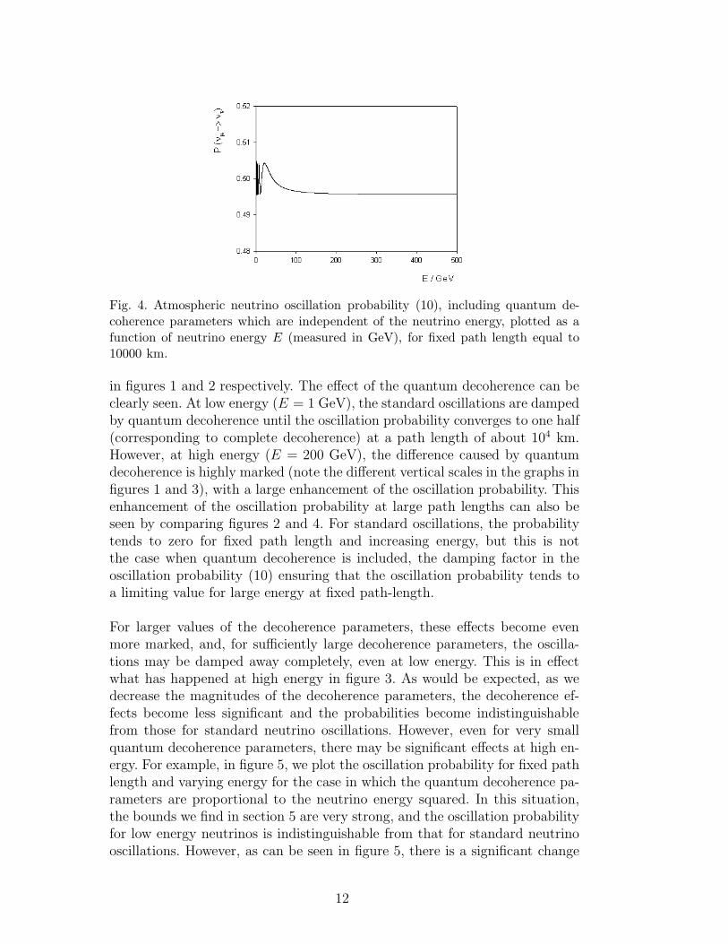
Fig. 4. Atmospheric neutrino oscillation probability (10), including quantum de-coherence parameters which are independent of the neutrino energy, plotted as afunction of neutrino energy E (measured in GeV), for fixed path length equal to10000 km.

in figures 1 and 2 respectively. The effect of the quantum decoherence can beclearly seen. At low energy (E = 1 GeV), the standard oscillations are dampedby quantum decoherence until the oscillation probability converges to one half(corresponding to complete decoherence) at a path length of about 104 km.However, at high energy (E = 200 GeV), the difference caused by quantumdecoherence is highly marked (note the different vertical scales in the graphs infigures 1 and 3), with a large enhancement of the oscillation probability. Thisenhancement of the oscillation probability at large path lengths can also beseen by comparing figures 2 and 4. For standard oscillations, the probabilitytends to zero for fixed path length and increasing energy, but this is notthe case when quantum decoherence is included, the damping factor in theoscillation probability (10) ensuring that the oscillation probability tends toa limiting value for large energy at fixed path-length.

For larger values of the decoherence parameters, these effects become evenmore marked, and, for sufficiently large decoherence parameters, the oscilla-tions may be damped away completely, even at low energy. This is in effectwhat has happened at high energy in figure 3. As would be expected, as wedecrease the magnitudes of the decoherence parameters, the decoherence ef-fects become less significant and the probabilities become indistinguishablefrom those for standard neutrino oscillations. However, even for very smallquantum decoherence parameters, there may be significant effects at high en-ergy. For example, in figure 5, we plot the oscillation probability for fixed pathlength and varying energy for the case in which the quantum decoherence pa-rameters are proportional to the neutrino energy squared. In this situation,the bounds we find in section 5 are very strong, and the oscillation probabilityfor low energy neutrinos is indistinguishable from that for standard neutrinooscillations. However, as can be seen in figure 5, there is a significant change

12

Fig. 5. Atmospheric neutrino oscillation probability including quantum decoherenceparameters which are proportional to the neutrino energy squared, plotted as afunction of neutrino energy E (measured in GeV), for fixed path length equal to10000 km.

in the neutrino oscillation probability at high energy.

The values of the quantum decoherence parameters used in producing figure 5are sufficiently small that they have not been ruled out by current atmosphericneutrino oscillation data [10]. It is clear from figure 5 that high energy neu-trinos are necessary in order to probe such quantum decoherence effects, andit is the main result of this paper that neutrino telescopes such as ANTARESare indeed able to perform this, in contrast to comparatively low-energy ex-periments. We would expect the bounds we discuss in section 5, attainablewith atmospheric neutrino data, to be further tightened with neutrinos ofastrophysical rather than atmospheric origin [41].

4 Specific Models of Quantum Decoherence

In this section we now discuss in detail specific models of quantum decoher-ence. The most general time evolution equation including quantum decoher-ence effects (5) involves six parameters additional to those for the standardneutrino oscillations. It is not possible to derive analytically in a simple closedform a general oscillation probability involving all six extra parameters, andeither a numerical approach or an approximation scheme would be necessary[5,6]. Furthermore, it is unlikely that, at least to begin with, experimental datawill be able to produce meaningful bounds/fits for all six additional parame-ters. In view of the above, we shall consider models in which only two or fewerof the quantum decoherence parameters α, β, δ, a, b, or d are non-zero, butwe study different combinations of these parameters in order to incorporatedifferent possible effects.

13

Various models have been considered in the literature to date (see, for example,[5,6,7,8,9]), although the only work of which we are aware involving analysis ofexperimental data is [10,11]. The models which have received most attentionto date are those with a, α and b non-zero but d, β and δ zero [5,7,8] andthose where α, β and δ are non-zero but a, b and d vanish [5,6,8,9]. Benattiand Floreanini [5] consider a quite general model (all parameters non-zero)initially, but later concentrate on the case when d = β = 0 and also δ = 0,although they impose the condition of complete positivity. They also considerall parameters non-zero using a second order approximation. Our models beloware all special cases of the models considered by Benatti and Floreanini. Liuand collaborators [6] set a = b = d = 0, although in this case the oscillationprobability can only be computed numerically. Here we either set both a and αto be zero, or both are non-zero, so our probabilities do not tally with theirs.Chang et al [8] consider the same model as [6], but set β = 0 in order toobtain an analytic probability. Again, our models do not fit into their picture.They also consider the leading order corrections to the standard oscillationprobability for a, b, and α non-zero and d, β, and δ vanishing. Ma and Hu [7]work with the second of Chang et al’s models, this time with exact analyticresults for the oscillation probability. Models 1 - 4 below consider variouscombinations of parameters within this model. Finally, Klapdor-Kleingrothausand collaborators [9] consider a model in which only α and δ are non-zero.

We first consider a class of models in which we set d and β equal to zero,so that both the terms M13(E, L) and M31(E, L) in equation (7) vanish. Theforms of the quantities M11(E, L) and M33(E, L) in equation (7) are derivedby solving the differential equations (6) describing the time evolution of thecomponents of the density matrix, using suitable initial conditions. The answer(with c = ~ = 1) is:

M11 =

e−Γsum cos Γ1 if a = α;

e−Γsum

(

cos Γ2 + Γdiff

Γ2sin Γ2

)

if b = 0;

M33 = e−2δL; (11)

with

Γsum =(α + a) L;

Γdiff =(α − a)L;

Γ1 =2

(

∆m2L

4E

)2

− b2L2

1

2

;

Γ2 =2

(

∆m2L

4E

)2

− 1

4(α − a)2 L2

1

2

. (12)

14

Setting the quantum decoherence parameters in equations (11-12) equal tozero, we recover the standard oscillation probability. The other limit of inter-est is if we set the standard oscillation parameter ∆m2 = 0 (but keeping theusual mixing angle θ non-zero). In this case atmospheric neutrino oscillationswould be due to quantum decoherence effects only. Given the widespread ac-ceptance of the standard oscillation picture, such a scenario may seem highlyunlikely, but the only existing analysis of experimental data [10,11] found that,while oscillations due to quantum decoherence only are unfavoured by the ex-perimental data, the evidence is not overwhelming. However, in this paper weshall mostly be concerned with quantum decoherence effects as modificationsof the standard picture. If we do set ∆m2 = 0 in equation (12), it is clearthat we can obtain a sensible oscillation probability only if Γ1 and Γ2 are real,which means that a = α and b = 0. If, however, Γ1 and Γ2 are imaginary when∆m2 = 0, it is possible to write the oscillation probability in terms of expo-nential (damping) terms only, without any oscillations. Given the success ofthe phenomenology of neutrino oscillations, we do not consider this possibilityfurther.

The parameter δ corresponds to energy non-conserving effects in the atmos-pheric neutrino system. However, since the terms in the probability (7) whichcontain δ are multiplied by cos2(2θ), and the current experimental best-fitvalue for cos2(2θ) is zero [11], this energy non-conserving parameter has anegligible effect on the oscillation probability, and so we will not consider itfurther in this section. However, see section 6 for bounds on this parameterfrom other experiments. The models of this first type we shall consider aretherefore:

(1) The simplest possible model is when b = δ = 0 and a = α 6= 0. It isthis model which has been studied for Super-Kamiokande and K2K data[10,11], and the time evolution of the density matrix satisfies the condi-tions of complete positivity and energy conservation within the atmos-pheric neutrino system. Furthermore, only in this model does the time-evolution of the density matrix (2) have the Lindblad form (3).

(2) We set b = δ = 0, with a and α non-zero but not equal. This is thesimplest possible generalization of the previous model; and energy is con-served in this case (as it is in the next two models as well). This modelis probably the most likely generalization to be of experimental signifi-cance, since the consensus in the literature is that b will be significantlysmaller than either a or α. However, this model violates the condition ofcomplete positivity [5]. In this and the following two models, oscillationscannot be accounted for solely by quantum decoherence, and we mustinclude a non-zero ∆m2 in the probability.

(3) In our third model we consider only a non-zero b in (12), setting all otherquantum decoherence parameters (including a and α) to vanish. Theform of the probability (7) is such that the sign of b cannot be measured,

15

so we assume from henceforth that b is positive (equivalently, we areconsidering only |b|). In the literature, the assumption is frequently madethat b will be much smaller than either a or α, which would rule thismodel out. However, we include it here so that we can look specificallyat the effect of b on the system. Like the previous model, this one alsoviolates complete positivity [5].

(4) Our next model is, in effect, a combination of the previous two. We seta = α and b to be non-zero, but have δ and all other quantum decoher-ence parameters vanishing. Even this more general model does not satisfycomplete positivity [5] as we have set δ = 0. In studying this model in thenext section, we find no additional information on the parameter spaceof α, a and b than we did by studying models 2 and 3, which implies thatit is sufficient to consider varying the quantum decoherence parametersseparately, at least as far as finding upper bounds on sensitivity regionsis concerned.

Our second class of models violate energy conservation within the atmosphericneutrino system. We set a = b = α = δ = 0 and consider instead non-zero dand β. The oscillation probability will have the general form (7). Although,because the mixing angle θ for atmospheric neutrino oscillations is such thatcos2(2θ) is very close to zero, we are unable to measure M33, M31 or M13

directly, there are, in the two models below, also modifications of M11 whichwe can probe, and so measure these other quantities indirectly. This is incontrast to the situation in which the parameter δ is non-zero, as this showsup only in M33 if d = β = 0. The models we consider are therefore:

(5) Firstly, we set all parameters equal to zero except β. The oscillationprobability (7) in this case is

P [νµ → ντ ] =1

2

cos2 2θ

[

1 − ω2

Ω2β

+β2

Ω2β

cos(2ΩβL)

]

+ sin2 2θ

[

1 +β2

Ω2β

− ω2

Ω2β

cos(2ΩβL)

]

(13)

where Ωβ =√

ω2 − β2 and ω = ∆m2

4E. In both this model and the next,

it is not possible for oscillations to be due to decoherence only, as theargument of the cos term becomes imaginary if we set ∆m2 = 0. Theprobability (13) contains only β2 terms and so we consider only β > 0(or, equivalently, |β|).

(6) In this model, we set all the quantum decoherence parameters to zeroexcept d. The probability of oscillation (7) in this case has the form:

16

P [νµ → ντ ] =1

2

cos2 2θ

[

1 − ω2

Ω2d

+d2

Ω2d

cos(2ΩdL)

]

+ sin2 2θ

[

1 +d2

Ω2d

cos(2ΩdL) − ω2

Ω2d

cos(2ΩdL)

]

+ sin 4θ

[

d

Ωd

sin(2ΩdL)

]

(14)

where Ωd =√

ω2 − d2. This is the only model in which the quantitiesM13(E, L) and M31(E, L) are non-zero. Although both d and d2 appearin the probability (14), in fact only d2 can be measured with atmosphericneutrinos because sin 4θ ∼ 0. Therefore we consider only d > 0 (or |d|).

We are now in a position to examine ANTARES sensitivity to these quantumdecoherence effects.

5 ANTARES sensitivity to quantum decoherence in atmospheric

neutrino oscillations

ANTARES is sensitive to high energy atmospheric neutrinos, with energyabove 10 GeV [13]. Although in some sense these are a background to theneutrinos of astrophysical origin which are the main study of a neutrino tele-scope, nevertheless the detection of very high energy atmospheric neutrinoswhich have very long path lengths (of the order of the radius of the Earth) iscomplementary to other long baseline neutrino experiments such as MINOS[24], OPERA [25], K2K [42], KamLAND [43] and CHOOZ [44]. Our analysisof the sensitivity of ANTARES to quantum decoherence effects in atmosphericneutrinos is based on a modification of the analysis of standard atmosphericneutrino oscillations with ANTARES [13,45]. We would anticipate that otherhigh energy neutrino telescopes such as AMANDA [20] and ICECUBE [21]would also be able to probe these effects.

5.1 Simulations and analysis

Our simulations are based on previous ANTARES simulations of the sensi-tivity to standard neutrino oscillations [45]. Further details of the ANTARESdetector, detector simulation and event signals can be found in [45]. Here wesummarize the main features of the simulations which are pertinent to ourdiscussion. Atmospheric neutrinos events were generated using Monte-Carloproduction. A spectrum proportional to E−2 for the neutrinos was assumed,for energies in the range 10 GeV < E < 100 TeV. The zenith angle distri-

17

bution is assumed to be isotropic. Twenty-five years of data were simulated,so that errors from the MC statistics could safely be ignored. Event weightswere used to adapt the MC flux to a real atmospheric neutrino flux. We usedthe Bartol theoretical flux [46], although the results will not be significantlychanged by using different theoretical fluxes. There may be a more significantchange in our results if the spectral index is modified.

Our simulations are based on three years’ data taking with ANTARES. Thiscorresponds to roughly 10000 atmospheric neutrino events. All errors arepurely statistical, with simple Gaussian errors assumed. By varying the formof the oscillation probability to include quantum decoherence effects, spectrain either E, E/L or L are produced. Some examples of these are discussed inthe next subsection. Since ANTARES is particularly sensitive to the zenithangle ϑ and thereby the path length L, the spectra in E/ cos ϑ are used in thesensitivity analysis.

To produce sensitivity regions, we used a χ2 technique, comparing the χ2

for oscillations with decoherence (or decoherence alone) with that for the no-oscillation hypothesis. The total normalization is left as a free parameter inthe sensitivity analysis, so that our results in section 5.3 are not affected bythe normalization of the atmospheric neutrino flux. The sensitivity regions atboth 90 and 99% confidence level are produced.

Even though our analysis is independent of the normalization of the atmos-pheric neutrino flux, in order to produce spectra based on numbers of events,as in the following subsection, some normalization of the total flux is neces-sary. For standard oscillations without quantum decoherence, bins with highE/ cos ϑ can be used to normalize the flux as standard oscillations are negli-gible at sufficiently high E/L (as can be seen in figure 1). This method canalso be applied for quantum decoherence models in which the decoherenceparameters are inversely proportional to the neutrino energy, so that decoher-ence also becomes negligible at high energy. However, when the decoherenceparameters are proportional to the neutrino energy squared, decoherence issignificant at high energies but negligible at low E/L. Therefore, in this lattercase, we may use the low E/ cos ϑ bins to normalize the flux.

We have studied six different models of quantum decoherence, as outlined inthe previous section, and for each model there are three different ways in whichthe quantum decoherence parameters may depend on the neutrino energy. Weshall not discuss the details of all eighteen of our simulations, but insteadsummarize our results and discuss a few models in more detail to illustratethe essential features. In our simulations, for practical reasons, we had at mostthree varying parameters, one of which was always the mixing angle θ whichfacilitated comparisons with previous work [10,11,45]. In models with only onenon-zero decoherence parameter (namely models 1, 3, 5 and 6 above) we also

18

varied ∆m2, to check that our sensitivity regions included the current best-fitvalues [10,11]. In models with two non-zero decoherence parameters (models2 and 4), we fixed ∆m2 = 2.6 × 10−3 eV2. The simulations then give us athree-dimensional region of sensitivity at 90 and 99 percent confidence level,and we plotted the boundaries of the projections of the surface bounding thisvolume onto the co-ordinate planes, where necessary also plotting the surfaceitself.

5.2 Spectra

As well as data based on total numbers of events, the spectra of these eventsin (typically) E/L is also important in neutrino oscillation physics. For atmos-pheric neutrinos, Super-Kamiokande [12] has reported an oscillatory signaturein the E/L spectrum of events, and similar spectral analyses have been per-formed for KAMLAND [23] and K2K [47]. As well as being used in our analysisof sensitivity regions, the spectra themselves are important for searching forpossible decoherence effects and also for bounding the size of such effects. Theoverall normalization of the flux, required to produce these spectra, can befound using either the high or low E/ cosϑ bins, depending on the situation,as described in the previous subsection.

Figures 6, 7 show typical spectra of events as a function of E/ cosϑ (cor-responding to E/L), where E is the reconstructed energy and ϑ the zenithangle, not to be confused with the mixing angle θ. In each case, the solid lineis the MC simulation with standard oscillations and no decoherence, using thevalues of the oscillation parameters in (9), while the dotted and dashed linesare the MC simulation with standard oscillations and decoherence together.The spectra in figure 6 are for the model in which the quantum decoherenceparameters are inversely proportional to the neutrino energy, while in figure7 we consider quantum decoherence parameters which are proportional to theneutrino energy squared. In both figures 6, 7, we have also plotted the ratioof the number of events compared with no oscillations. It can be seen that inboth cases quantum decoherence results in a significant reduction in the num-ber of events. However, there is also a difference in the shape of the spectra. Inboth models, when the decoherence parameters are comparatively large, thespectrum in the ratio of the number of events (lower plots) is much flatter inthe region below about 150 GeV, compared with standard oscillations (whenthere is a ‘dip’ in the ratio of the number of events). For the case in whichthe decoherence parameters are inversely proportional to the neutrino energy,the ratio of the number of events rises to one at very high energies, but moreslowly than the case of oscillations only. However, it should be stressed thatthe values of the parameter µ2 for which this is most noticeable in figure 6 arelarger than the current best upper bound from SK and K2K data [11]. When

19

Fig. 6. Spectrum of events as a function of E/ cos ϑ (top) and ratio of the numberof events compared to no oscillations (bottom). In each graph, the solid line repre-sents MC simulation of standard oscillations without decoherence, and the dottedlines represent MC simulation of standard oscillations plus decoherence. The datapoints correspond to a three-year measurement, assuming standard oscillations onlywithout decoherence. The decoherence parameters are inversely proportional to theneutrino energy.

the decoherence parameters are proportional to the neutrino energy squared(figure 7), the spectrum of the ratio of the number of events is extremely flat.

We can also consider the situation in which there are no standard oscilla-tions, in other words, the squared mass difference ∆m2 is zero. In this case,neutrino oscillations would be described entirely by decoherence. In this casethe ratios of the numbers of events compared with the no-oscillation hypoth-esis are shown in figure 8, for decoherence parameters inversely proportional

20

Fig. 7. Spectra of events as in figure 6 but for the case when the decoherenceparameters are proportional to the neutrino energy squared.

to the neutrino energy (upper plot) and proportional to the neutrino energysquared (lower plot). We have plotted in figure 8 the ratio for the standardoscillations only case for comparison (the solid line), but the other curvesare for pure decoherence without standard oscillations. The difference in thespectra at E/ cos ϑ below about 150 GeV is clear for the case when the de-coherence parameters are proportional to the neutrino energy squared, withthe decoherence-only model generally producing a peak in the spectrum wherestandard oscillations without decoherence has a dip. When the decoherenceparameters are inversely proportional to the neutrino energy, the spectra lookmore like those for standard oscillations plus decoherence (figure 6), except forsmall values of µ2, when the spectrum is flatter than for standard oscillationsonly.

21

Fig. 8. Ratios of the number of events compared to no oscillations, as functions ofE/ cos ϑ. The solid line is for standard oscillations only without decoherence, forcomparison. The remaining curves are for no standard oscillations, and quantumdecoherence only. The upper plot is for quantum decoherence parameters inverselyproportional to the neutrino energy, and the lower plot for the case when the quan-tum decoherence parameters are proportional to the neutrino energy squared.

It should be emphasised that the values of the quantum decoherence parameterκ used to generate the spectra in figures 7 and 8 are many orders of magnitudesmaller than the current experimental upper bound of 10−19 eV−1 [10]. As thedecoherence parameter κ increases, the number of events decreases and so itis clear from figures 7 and 8 that ANTARES will be able to rule out even verysmall values of κ. This can be understood from the oscillation probabilitiesas shown in the figures in section 3. For high energy neutrinos, the standardoscillation probability is negligible and so the number of events depends only

22

on the atmospheric neutrino flux. However, with quantum decoherence, theoscillation probability becomes close to one-half for atmospheric neutrinos andso a large fraction of the incoming muon neutrinos will oscillate, resulting in asignificant decrease in the number of events seen. For low energy neutrinos, asobserved by current atmospheric neutrino experiments, in the model we haveconcentrated on in this subsection, the effects of quantum decoherence arenegligible with these values of the quantum decoherence parameters becausethe effects are proportional to the neutrino energy squared.

This is the main result of our paper: ANTARES measures high-energy neu-trinos and so will be able to put stringent bounds on quantum decoherenceeffects which are proportional to the neutrino energy squared.

5.3 Sensitivity regions

We now turn to a discussion of the ANTARES sensitivity regions from oursimulations. We discuss the simplest model in some detail as it reveals mostof the salient features. The remaining models are summarized briefly. We areparticularly interested in the upper bounds on the sensitivity regions. We focusmainly on the case where the quantum decoherence parameters are propor-tional to the neutrino energy squared, as here we will have the most significantimprovement on current experimental bounds.

5.3.1 Model 1

This is the model in which α = a and has been studied for Super-Kamiokandeand K2K data [10,11]. They found the best fit to the data when the quantumdecoherence parameter is inversely proportional to the neutrino energy [10].A detailed analysis [11] of this case then found that the favoured situationwas standard oscillations without decoherence, but that the data could notentirely rule out oscillations due to quantum decoherence only. We show ourresults for this model with the parameters α = a inversely proportional tothe neutrino energy in detail for comparison purposes, but our main resultsare concerned with the case in which the parameters are proportional to theneutrino energy squared, as it is in this latter case that we can significantlyimprove current bounds.

Firstly, consider the case in which ∆m2 = 0, so that there are no standardoscillations and only quantum decoherence. Figure 9 shows the sensitivitycurves in this case, for α = a inversely proportional to the neutrino energy, andfigure 10 for α = a proportional to the neutrino energy squared. It is somewhatsurprising that current experimental data [11] only slightly disfavours thismodel, in comparison to the standard oscillation picture. The best fit value

23

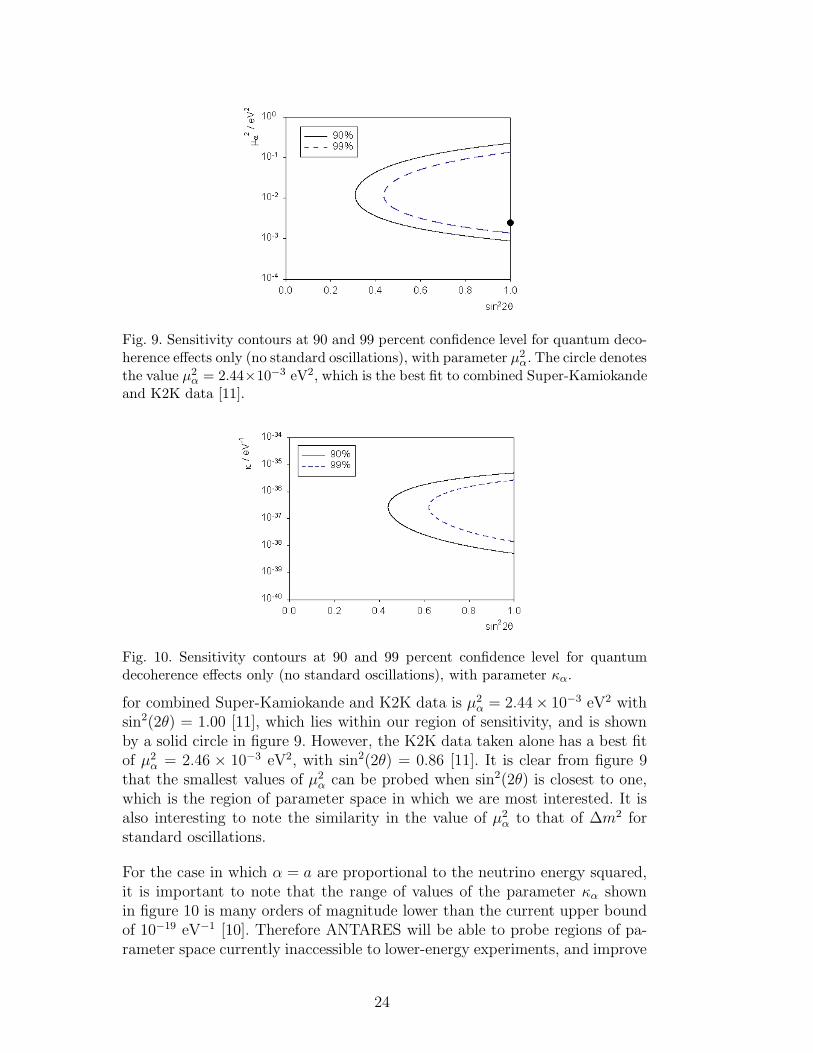
Fig. 9. Sensitivity contours at 90 and 99 percent confidence level for quantum deco-herence effects only (no standard oscillations), with parameter µ2

α. The circle denotesthe value µ2

α = 2.44×10−3 eV2, which is the best fit to combined Super-Kamiokandeand K2K data [11].

Fig. 10. Sensitivity contours at 90 and 99 percent confidence level for quantumdecoherence effects only (no standard oscillations), with parameter κα.

for combined Super-Kamiokande and K2K data is µ2α = 2.44× 10−3 eV2 with

sin2(2θ) = 1.00 [11], which lies within our region of sensitivity, and is shownby a solid circle in figure 9. However, the K2K data taken alone has a best fitof µ2

α = 2.46 × 10−3 eV2, with sin2(2θ) = 0.86 [11]. It is clear from figure 9that the smallest values of µ2

α can be probed when sin2(2θ) is closest to one,which is the region of parameter space in which we are most interested. It isalso interesting to note the similarity in the value of µ2

α to that of ∆m2 forstandard oscillations.

For the case in which α = a are proportional to the neutrino energy squared,it is important to note that the range of values of the parameter κα shownin figure 10 is many orders of magnitude lower than the current upper boundof 10−19 eV−1 [10]. Therefore ANTARES will be able to probe regions of pa-rameter space currently inaccessible to lower-energy experiments, and improve

24

significantly on existing experimental bounds.

We also studied pure decoherence for the case in which α = a do not dependon the neutrino energy. The sensitivity curves in this case have a very similarshape to those in figures 9 and 10, with sensitivity to values of the parameterγα in the region 10−13 – 10−14 eV, which is a similar range to the current upperbound from SK data of 10−14 eV [10].

We also found sensitivity curves for the more general case when both ∆m2

and µ2α, κα or γα (as applicable) are non-zero. The results we obtained are

shown in figures 11 and 12 for the µ2α and κα cases, respectively. We do not

show the graphs for the γα case because they are qualitatively very similarto the µ2

α case. In figures 11 and 12, we have plotted projections of a three-dimensional volume onto each of the co-ordinate planes, and the contoursrepresent the boundaries of the projected regions. The sensitivity contoursshould be compared with the combined Super-Kamiokande and K2K results[11]. In each figure, the best fit values of ∆m2 = 2.6×10−3 eV2 and sin2(2θ) = 1[11] are denoted by a triangle, while the upper bound µ2

α < 3 × 10−3 eV2 [11]is marked by a dotted line in figure 11. Our regions have a very similar shapeto those constructed from data in [11].

For the situation in which the quantum decoherence parameters are inverselyproportional to the neutrino energy (figure 11), it should be noted that theupper bound on the sensitivity region at sin2(2θ) = 1 is considerably higherthan the upper bound from data [11]. This is to be expected since ANTARESmeasures only high energy atmospheric neutrinos (energy greater than 10 GeVcompared with a few GeV for Super-Kamiokande [48] and K2K [42]) and so islikely to be comparatively insensitive to effects inversely proportional to theneutrino energy. However, when the decoherence parameters are proportionalto the neutrino energy squared (figure 12), the upper bound on the sensitivityregion, κα < 10−35 eV −1, is many orders of magnitude smaller than thecorresponding bound from Super-Kamiokande data of 10−19 eV−1 [10]. In thefinal case, when the quantum decoherence parameters are independent of theneutrino energy, we find an upper bound on the sensitivity region of γα <10−14 eV, which is of a similar order of magnitude to the bound from Super-Kamiokande data of 10−14 eV [10].

5.4 Models 2, 3 and 4

These models involve combinations of the quantum decoherence parametersa, α and b. The upper bounds of the sensitivity regions that we find for aparticular parameter are essentially independent of the particular combinationof other parameters chosen to be non-zero, and whether or not we fix ∆m2.

25

Fig. 11. Sensitivity contours at 90 and 99 percent confidence level, when both os-cillation and quantum decoherence parameters (µ2

α) are non-zero. The dotted linedenotes the bound µ2

α < 3× 10−3 eV2 from Super-Kamiokande and K2K data [11],and the triangle the best fit value ∆m2 = 2.6 × 10−3 eV2, sin2(2θ) = 1 [11].

The parameters a and α have the same sensitivity regions when they are notnecessarily equal, and whenever the parameter b is included, it has a upperbound corresponding to the value at which the factors Γ1 and Γ2 (12) (asapplicable) become imaginary.

26

Fig. 12. Sensitivity contours at 90 and 99 percent confidence level, when both oscil-lation and quantum decoherence parameters (κα) are non-zero. The triangle denotesthe best fit value ∆m2 = 2.6 × 10−3 eV2, sin2(2θ) = 1 [11].

As an illustration of our results in these models, we plot in figure 13 thesensitivity curves for the model in which a = α 6= 0, b 6= 0, ∆m2 is fixedat its best fit value (9) [11], and with the quantum decoherence parametersproportional to the neutrino energy squared, as it is in this case that we havethe most stringent bounds on quantum decoherence effects. We find upper

27

Fig. 13. Sensitivity contours at 90 and 99 percent confidence levels, with twonon-zero decoherence parameters which are proportional to the neutrino energysquared and given in terms of the constants κs = κα = κa and κb.

bounds on the sensitivity regions of κs = κa = κα < 10−38 eV−1 and κb < 10−45

eV−1. As with model 1, these bounds are very strong, and it is interesting tonote that our bound on κa = κα is a couple of orders of magnitude smaller inthis model than it was in model 1.

28

If the quantum decoherence parameters are independent of the neutrino en-ergy, we find upper bounds to our sensitivity regions of γa = γα < 10−13 eVand γb < 10−16 eV, this latter value again being due to the cut-off in b. Forthe third possibility, when the quantum decoherence parameters are inverselyproportional to the neutrino energy, our upper bounds are somewhat weaker,at µ2

α = µ2a < 100 eV2, and µ2

b < 10−2 eV2.

5.4.1 Model 5

To illustrate the typical sorts of plots we get for the sensitivity curves, we showin figure 14 the sensitivity contours for this model in the case in which thequantum decoherence parameter proportional to the neutrino energy squaredand given by κβ. There is again a cut-off in the parameter κβ due to theprobability (13) becoming imaginary, and this can be clearly seen in the plots.Our upper bound on κβ is 10−43 eV−1 in this case. The plots shown in figure14 are typical of those found in many of our models for the different quantumdecoherence parameters, when we also vary ∆m2.

When the quantum decoherence parameters are independent of the neutrinoenergy, the sensitivity regions are qualitatively the same as those in figure 14,and we find an upper bound γβ < 10−15 eV. However, when the quantumdecoherence parameters are inversely proportional to the neutrino energy, thesituation is rather more complicated, and we need to examine the surface inthree-dimensional parameter space which bounds the sensitivity region. Thisis shown in figure 15 for 90% confidence level. The region of interest lies abovethe surface in figure 15, including the value sin2(2θ) = 1. For small values ofµ2

β, it is clear that this region is similar in shape to the previous figure 14.However, for larger values of µ2

β, the surface opens out and all values of ∆m2

and sin2(2θ) are included. Because of this, we are unable to place an upperbound on µ2

β in this case. This is not entirely unexpected because ANTARESmeasures high energy neutrinos, so that its ability to place bounds on effectsinversely proportional to neutrino energy is limited.

5.4.2 Model 6

This model is somewhat different to any considered before as the parameterd is non-zero and so the oscillation probability (14) has contributions fromthe sin 4θ term. However, the sensitivity regions are broadly similar to thosein the previous model. We find the following upper bounds on the sensitivityregions:

γd < 10−15 eV; µ2

d < 10−1 eV2; κd < 10−43 eV−1.

29

Fig. 14. Sensitivity contours at 90 and 99 percent confidence levels, for model 5 withboth standard oscillations and non-zero decoherence parameter κβ . The triangleshows the experimental point of best fit for ∆m2 [11].

6 Comparing experimental bounds on decoherence parameters

In this section we compare our upper bounds on quantum decoherence pa-rameters, from simulations, with existing experimental data. Firstly, for ease

30

Fig. 15. The boundary of the volume in parameter space at 90% confidence level,for model 5 with both standard oscillations and a non-zero decoherence parameterµ2

β. The sensitivity region lies above this surface.

model a |b| |d| α |β|

γ(GeV) 9 × 10−23 7 × 10−25 7 × 10−25 9 × 10−23 7 × 10−25

µ2(GeV2) 2 × 10−19 6 × 10−19 6 × 10−19 2 × 10−19 -

κ(GeV−1) 4 × 10−26 7 × 10−35 7 × 10−35 4 × 10−26 7 × 10−35

Table 1Table showing the upper bounds of the constants of proportionality in the quantumdecoherence parameters from simulations for different dependences on the neutrinoenergy.

of comparison, we restate, in table 1, the upper bounds of the constants ofproportionality γ, µ2 and κ for each of the quantum decoherence parame-ters, changing the units to GeV for ease of comparison with other references.Upper bounds have been placed on the decoherence parameters [10,11] byexamining data from the Super-Kamiokande and K2K experiments. We notethan the bounds for the γ model (γα < 3.5 × 10−23 GeV) are entirely con-sistent with those found in our simulations, the bounds for the µ2 model(µ2

α < 2.44 × 10−21 GeV2) are slightly better than the ANTARES boundswhereas the bounds found for the κ model (κα < 9× 10−10 GeV−1) are muchworse than our bounds. The ANTARES bounds are found with high energyneutrinos whereas Super-Kamiokande detects lower energy neutrinos and sowe see that experiments which are more sensitive to lower energy neutrinos arebetter probes of the µ2 model whilst those with sensitivity to higher energyneutrinos are much better at placing bounds on the quantum gravity param-eters using the κ model. For each quantum decoherence parameter, our upperbounds on the constant κ are particularly strong, and, given that κ containsone inverse power of the Planck mass (1019 GeV), are close to ruling out sucheffects.

The neutrino system is not the only quantum system which may be affected

31

by interactions with space-time foam. Experiments such as CPLEAR [49] haveexamined this problem with neutral kaons, and found the upper bounds onthe quantum decoherence parameters to be [50]

a < 4 × 10−17 GeV, |b| < 2.3 × 10−19 GeV, α < 3.7 × 10−21 GeV.

A second analysis of this experiment took place in reference [19] with sixquantum decoherence parameters. The authors of reference [19] were able toput bounds all the parameters and they found upper bounds on the quantumdecoherence parameters to be of order 10−17 − 10−18 GeV. It is difficult todirectly compare our results with these bounds due to the dependence on theneutrino energy in some of our models. However, when the quantum decoher-ence parameters are constants, our upper bounds on γ from table 1 lead toupper bounds on the decoherence parameters themselves of

a = α < 5 × 10−23 GeV, |b| = |d| = |β| < 3 × 10−25 GeV,

and so, it seems that the ANTARES experiment will be able to improve theupper bounds of these parameters with respect to the CPLEAR experiment.

Quantum decoherence has also been explored using neutron interferometryexperiments, as suggested in [4]. In reference [51], upper bounds on the pa-rameters a and α were found using data from such an experiment:

a ≤ 1 × 10−22 GeV, α ≤ 7.4 × 10−22 GeV.

Once again, our upper bounds are tighter than these values. It is interesting tonote that in both the kaon and neutron experiments, the quantum decoherenceparameter a 6= α whereas in the neutrino system, we find a = α. This variationarises from the different mixing in these systems. The other difference betweenthe meson and neutrino experiments is the possibility of different decoherenceeffects in the anti-neutrino sector as compared with the neutrino sector [35,36],although we have not considered this possibility further in this paper.

7 Other effects on atmospheric neutrino oscillations

Quantum decoherence is not the only process which may modify the standardoscillation probability (8) for atmospheric neutrinos. In this section we brieflydiscuss some of the other possible phenomena, indicating how they change theoscillation probability. We will then compare these effects with those comingfrom quantum decoherence.

The derivations of the oscillation probabilities have all been done within theframework of standard quantum mechanics. It has been suggested, however,

32

that approaching this problem from a quantum field theory (QFT) standpointcould alter the phenomenology [52,53]. This approach yields statistical aver-ages, but if we interpret these as probabilities, then there will be a modificationof the standard oscillation probability. However, the magnitude of the correc-tion is several orders of magnitude smaller than the size of the corrections dueto quantum decoherence that we are probing here.

There are other new physics effects which may alter the standard atmosphericneutrino oscillation probability, not just quantum decoherence. For example, ithas been suggested that our universe may have more than the 3+1 dimensionswe observe and that some of these extra dimensions may be large (see [54] foran introduction), which implies that we live on a four dimensional hyper-surface, a brane, embedded in a higher dimensional bulk. Adding large extradimensions gives rise to the possibility that some particles may propagateoff our brane through the bulk and it has been suggested that one of theseparticles may be a sterile neutrino into which the three familiar neutrinos couldoscillate. If we consider the mixing between the three standard neutrinos andthe sterile neutrino to simply be an extension of the three neutrino systemto a four neutrino system, and assuming that E1,2 << E3 << E4, then theprobability a muon neutrino oscillates into a tau neutrino is

P [νµ → ντ ] = 4Uµ3Uτ3(Uµ3Uτ3 + Uµ4Uτ4) sin2

[

∆m232

4EL

]

+4U2

µ4U2

τ4sin2

[

∆m243

4EL

]

.

Here, the probability has an extra term as we now have two large mass differ-ences. However, the quantities Uxi are constants, independent of E and L andhence, this simple model gives rise to different types of terms than those foundin equation (7). Similar corrections to the two-neutrino oscillation probabilityalso arise if we consider normal three-neutrino oscillations, but in this case thecorrections are very small.

It has, however, also been suggested that the sterile neutrino may not mix inthe standard way and that the the oscillation probability is instead [55]:

P [νa → νb] = 4U2

a3U2

b3e−

π2ξ23

2 sin2

[

∆m232

4EL

]

+23∑

l=1

Ua3Ub3UalUbl

∞∑

n=1

U2

0n cos

[

(λ2n − ξ2

ll)L

2ER2

]

+U2

a3U2

b3

∣

∣

∣

∣

∣

∞∑

n=1

U2

0ne−iλ2

n

2ER2 L

∣

∣

∣

∣

∣

2

(15)

33

where R is the size of the extra dimensions, ξi = miR are assumed to be small,ll = 2 if l = 1, 2 or ll = 3 if l = 3 and the U ’s are constants. This oscillationprobability has a different form to that in equation (7) as the exponential term

multiplies the sin2[

∆m2

4EL]

as opposed to the cos term. Also, if we assume that

R does not change with time, then the exponential term in equation (15) is aconstant whereas the exponential term in equation (7) is a function of E andL.

Another way in which quantum gravity is expected to modify neutrino physicsis through violations of Lorentz invariance [14,16]. As with non-standard sterileneutrinos, this leads to modifications of the oscillation probability which havea different form from those due to quantum decoherence. We will examine in aseparate publication the precise nature of these effects on atmospheric neutrinooscillations and whether these can be probed by ANTARES. Other types ofLorentz-invariance and CPT-violating effects (also known as “Standard ModelExtensions” (SMEs)) have been studied by Kostelecky and Mewes [56], andagain we shall return to these for ANTARES in the future. One side-effect ofSMEs is that, even for atmospheric neutrinos, matter interactions can becomesignificant. However, it has been shown that these can safely be ignored forneutrino energies above the scale of tens of GeV [57], which is the energy rangeof interest to us here.

Finally, more conventional physics may have an effect on atmospheric neutrinooscillations as measured by a neutrino telescope. For example, uncertainties inthe energy and path length of the neutrinos may lead to modifications of theoscillation probability which are similar in form to those arising from quan-tum decoherence [34,35] and interactions in the Earth may also be a factor.However, both these effects decrease as the neutrino energy increases, whereasour strongest results are for quantum decoherence effects which increase withneutrino energy.

8 Conclusions

In the absence of a complete theory of quantum gravity, phenomenological sig-natures of new physics are useful for experimental searches. In this article wehave examined one expected effect of quantum gravity: quantum decoherence.We have considered a general model of decoherence applied to atmosphericneutrinos, and simulated the sensitivity of the ANTARES neutrino telescopeto the decoherence parameters in our model. We find that high-energy atmos-pheric neutrinos are able to place very strict constraints on quantum deco-herence when the decoherence parameters are proportional to the neutrinoenergy squared, even though such effects are suppressed by at least one powerof the Planck mass. It should be stressed that although our results here are

34

for the ANTARES experiment, we expect that other high-energy neutrino ex-periments (such as ICECUBE and AMANDA) should also be able to probethese models.

Acknowledgements

This work was supported by PPARC, and DM is supported by a PhD stu-dentship from the University of Sheffield. We would like to thank Keith Hanna-buss and Nick Mavromatos for helpful discussions.

References

[1] L. Smolin, How far are we from the quantum theory of gravity?, Preprinthep-th/0303185.

[2] G. Amelino-Camelia, Introduction to quantum gravity phenomenology, Preprintgr-qc/0412136.

[3] N. Arkani-Hamed, S. Dimopoulos and G.R. Dvali, Phys. Lett. B429 263 (1998);L. Randall and R. Sundrum, Phys. Rev. Lett. 83 3370 (1999);L. Randall and R. Sundrum, Phys. Rev. Lett. 83 4690 (1999).

[4] J.R. Ellis, J.S. Hagelin, D.V. Nanopoulos and M. Srednicki, Nucl. Phys. B241

381 (1984).

[5] F. Benatti and R. Floreanini, J. High. Energy Phys. 02 032 (2000).

[6] Y. Liu, L-Z. Hu and M-L. Ge, Phys. Rev. D56 6648 (1997).

[7] F-C. Ma and H-M. Hu, Testing quantum mechanics in neutrino oscillation,Preprint hep-ph/9805391 (1998).

[8] C-H. Chang, W-S. Dai, X-Q. Li, Y. Liu, F-C. Ma and Z-J. Tao, Phys. Rev. D60

033006 (1999).

[9] H.V. Klapdor-Kleingrothaus, H. Pas and U. Sarkar, Eur. Phys. J. A8 577(2000).

[10] E. Lisi, A. Marrone and D. Montanino, Phys. Rev. Lett. 85 1166 (2000).

[11] G.L. Fogli, E. Lisi, A. Marrone and D. Montanino, Phys. Rev. D67 093006(2003).

[12] Y. Ashie et. al. (Super-Kamiokande Collaboration) Phys. Rev. Lett. 93 101801(2004).

35

[13] E.V. Korolkova (for the ANTARES collaboration), Nucl. Phys. Proc. Suppl.

136 69 (2004).

[14] N.E. Mavromatos, On CPT symmetry: Cosmological,

quantum-gravitational and other possible violations and their phenomenology,Preprint hep-ph/0309221.N.E. Mavromatos, Neutrinos and the phenomenology of CPT violation, Preprinthep-ph/0402005.N.E. Mavromatos, CPT violation and decoherence in quantum gravity, Preprintgr-qc/0407005.

[15] R. Brustein, D. Eichler and S. Foffa, Phys. Rev. D65 105006 (2002).

[16] J. Alfaro, H.A. Morales-Tecotl and L.F. Urrutia, Phys. Rev. Lett. 84 2318(2000).

[17] S. Choubey and S.F. King, Phys. Rev. D67 073005 (2003).

[18] J.R. Ellis, J.L. Lopez, N.E. Mavromatos and D.V. Nanopoulos, Phys. Rev. D53

3846 (1996).

[19] F. Benatti and R. Floreanini, Phys. Lett. B401 337 (1997).

[20] E. Andres et. al. Nature 410 441 (2001).

[21] J. Ahrens et. al., Astropart. Phys. 20 507 (2004).

[22] S.E. Tzamarias, Nucl. Instrum. Meth. A502 150 (2003).

[23] T. Araki et. al. (KAMLAND collaboration) Phys. Rev. Lett. 94 081801 (2005).

[24] P.J. Litchfield, Nucl. Instrum. Meth. A451 187 (2000).

[25] M. Komatsu, Nucl. Instrum. Meth. A503 124 (2003).

[26] M. Blennow, T. Ohlsson and W. Winter, J. High Energy Physics 0506 049(2005).

[27] J.A. Wheeler, Superspace and the nature of quantum geometrodynamics, inBattelle Rencontres: 1967 Lectures in Mathemetical Physics edited by C.DeWitt and J.A. Wheeler (W. A. Benjamin, New York, 1968).

[28] S.W. Hawking, Commun. Math. Phys. 43 199 (1975).

[29] S.W. Hawking, Commun. Math. Phys. 87 395 (1982).

[30] G. Lindblad, Commun. Math. Phys. 48 119 (1976).

[31] G.C. Ghirardi, A. Rimini and T. Weber, Phys. Rev. D34 470 (1986).

[32] E. Joos, H.D. Zeh, C. Kiefer, D. Giulini, J. Kupsch and I.-O. Stamatescu,Decoherence and the appearance of a classical world in quantum theory, Springer(1996).

[33] R. Gambini, R.A. Porto and J. Pullin, Class. Quantum Gravity 21 L51 (2004).

36

[34] T. Ohlsson, Phys. Lett. B502 159 (2001).

[35] G. Barenboim and N.E. Mavromatos, Phys. Rev. D70 093015 (2004).

[36] G. Barenboim and N.E. Mavromatos, J. High Energy Physics 0501 034 (2005).

[37] J.R. Ellis, N.E. Mavromatos, D.V. Nanopoulos and E. Winstanley, Mod. Phys.

Lett. A12 243 (1997).J.R. Ellis, N.E. Mavromatos and D.V. Nanopoulos, Mod. Phys. Lett. A12 1759(1997).J.R. Ellis, P. Kanti, N.E. Mavromatos, D.V. Nanopoulos and E. Winstanley,Mod. Phys. Lett. A13 303 (1998).

[38] R.C. Myers and M. Pospelov, Phys. Rev. Lett. 90 211601 (2003).

[39] S.L. Adler, Phys. Rev. D62 117901 (2000).

[40] G. Battistoni, A. Ferrari, T. Montaruli and P.R. Sala, Astropart. Phys. 19 269(2003); ibid 19 291 (2003).C.G.S. Costa, Astropart. Phys. 16 193 (2001).

[41] D. Hooper, D. Morgan and E. Winstanley, Phys. Lett. B609 206 (2005).D. Hooper, D. Morgan and E. Winstanley, Phys. Rev. D72 065009 (2005).

[42] M.H. Ahn et. al. (K2K Collaboration), Phys. Rev. Lett. 90 041801 (2003).

[43] K. Eguchi et. al. (KamLAND Collaboration), Phys. Rev. Lett. 90 021802 (2003).

[44] M. Apollonio et. al., Phys. Lett. B420 397 (1998).

[45] F. Blondeau and L. Moscoso (ANTARES collaboration), Detection of

atmospheric neutrino oscillations with a 0.1 km2 detector : the case for

ANTARES NOW 98 conference, Amsterdam, Netherlands (1998).J. Brunner (ANTARES collaboration), Measurement of neutrino oscillations

with neutrino telescopes, 15th International Conference On Particle And Nuclei(PANIC 99), Uppsala, Sweden (1999).C. Carloganu (ANTARES collaboration), Nucl. Phys. Proc. Suppl. 100 145(2001).

[46] T.K. Gaisser, M. Honda, P. Lipari, T. Stanev, Primary spectrum to 1 TeV

and beyond, International Conference on Cosmic Rays (ICRC 2001), Hamburg,Germany (2001).

[47] E. Aliu et. al. (K2K Collaboration), Phys. Rev. Lett. 94 081802 (2005).

[48] Y. Fukuda et. al. (SuperKamiokande Collaboration), Phys. Lett. B433 9 (1998).

[49] CPLEAR Collaboration, Phys. Rep. 374 165 (2003).

[50] J. Ellis and CPLEAR Collaboration, Phys. Lett. B364 239 (1995).

[51] F. Benatti and R. Floreanini, Phys. Lett. B451 422 (1999).

37

[52] M. Blasone, P.A. Henning and G. Vitiello, Phys. Lett. B451 140 (1999).M. Blasone and G. Vitiello, Quantum field theory of particle mixing and

oscillations, Preprint hep-ph/0309202.

[53] K.C. Hannabuss and D.C. Latimer, J. Phys. A33 1369 (2000).K.C. Hannabuss and D.C. Latimer, J. Phys. A36 L69 (2003).

[54] G. Gabadadze, ICTP Lectures on Large Extra Dimensions, Preprinthep-ph/0308112.

[55] R. Barbieri, P. Creminelli and A. Strumia, Nucl. Phys. B585 28 (2000).

[56] V.A. Kostelecky and M. Mewes, Phys. Rev. D69 016005 (2004).V.A. Kostelecky and M. Mewes, Phys. Rev. D70 031902 (2004).

[57] M. Jacobson and T. Ohlsson, Phys. Rev. D69 013003 (2004).

38