practise: robust prediction of data center time series

PRACTISE: Robust Prediction of Data Center Time Series

Ji Xue∗, Feng Yan∗, Robert Birke†, Lydia Y. Chen†, Thomas Scherer†, and Evgenia Smirni∗

∗College of William and Mary

Williamsburg, VA, USA

{xuejimic,fyan,esmirni}@cs.wm.edu†IBM Research Zurich Lab

Zurich, Switzerland

{bir,yic,tsc}@zurich.ibm.com

Abstract—We analyze workload traces from production datacenters and focus on their VM usage patterns of CPU, memory,disk, and network bandwidth. Burstiness is a clear characteristicof many of these time series: there exist peak loads within clearperiodic patterns but also within patterns that do not have clearperiodicity. We present PRACTISE, a neural network basedframework that can efficiently and accurately predict futureloads, peak loads, and their timing. Extensive experimentationusing traces from IBM data centers illustrates PRACTISE’ssuperiority when compared to ARIMA and baseline neural net-work models, with average prediction errors that are significantlysmaller. Its robustness is also illustrated with respect to theprediction window that can be short-term (i.e., hours) or long-term (i.e., a week).

I. INTRODUCTION

Effective workload characterization and prediction hold theanswers to the conundrum of efficient resource allocation indistributed and scaled out systems. Being able to accuratelypredict the upcoming workload within the next time frame(i.e., in the next 10 minutes, half hour, hour, or even week)allows the system to make proactive decisions, rather thanreactive ones. Proactive decisions can be used with superiorperformance in storage systems by timely warming up thecache with the working set [1], [2], especially in systemswhere traditional internal work (e.g., garbage collection, snap-shots, upgrades) is interleaved with the user workload duringopportune times. Proactive scheduling of data analytics workcan result in personalized advertising, sentiment analysis, ortimely product recommendation, i.e., before the user leavesthe site [3], [4], [5]. Virtual machine (VM) consolidation andmigration is another example where accurate prediction of thephysical machine utilizations can guide effective system usage[6], [7], [8]. In all of the above cases, prediction of the intensityof peak loads and of their timings becomes key to the effectivelaunching of proactive management.

To maintain performance at tails, e.g., at high percentilesof response times, resource management policies [3], [6], [8],need to address the demands of peak loads instead of averageloads only. Depending on the capability of predicting peakload magnitudes and timings, resources can be multiplexed atvarious degrees across users and across time. Such predictionscan guide VM consolidation in data centers.

In this paper, we focus on data center workloads within theprivate cloud operated by IBM and used by major corporationsfor their IT needs. Prior work on workload characterizationat IBM data centers [9] focused on statistical analysis ofthe usage of specific components of the virtual and physical

machines, e.g., CPU and IO [9], [10]. This statistical analysisfocused on averages, percentiles, and trends, aiming to abetter understanding of how the workload evolves across atwo-year period, but largely ignored the time series of thevarious performance metrics. In this paper, we focus on thesetime series and develop methodologies for accurate predictionof various workload metrics and especially peaks and theirtimings.

Classic time series models such as ARIMA [11] can beused for online prediction. Such models first need to betrained using past observations and can predict the upcomingworkload. Alternatively, neural networks can be used in thesame manner and provide a black box approach to predict thefuture, especially to predict events that have been observed inthe past. Superior to the classic time series models that use alinear basis function, neural networks model input using non-linear functions, which improves their ability to handle morecomplex observations. Features gathered from observations arenot all equally informative; some are relevant, while othersare noise. Key to effective neural network prediction is thediscovery of the appropriate features. Neural network trainingis then conducted based on these.

In this paper, we develop a robust framework for predictionof data center time series (PRACTISE) and illustrate theflexibility of such a black box approach by showing remarkableaccuracy in usage prediction of data center workloads in thewild. We focus on four components: CPU, memory, disk,and network. We focus on an actual production workload andparticularly on 56 physical machines that host 775 virtual ma-chines during a time period of 61 days. Based on observationsof the workload pattern and its periodicity, we extract thefeatures that identify the time periods in which the repetitivepatterns occur. We also develop a bagging module [12] andan online updating module to improve the stability, accuracy,and speed of PRACTISE. We provide detailed comparisonswith ARIMA and show that the proposed black box approachoffers a significant improvement in predicting resource usage,by reducing average errors by three times. PRACTISE slashesthe false negative prediction rates of peak loads to less than12% and achieves two fold to nine fold improvements in theaccuracy of timing predictions. PRACTISE is lightweight andachieves training and prediction by an order of magnitudefaster than other methods, which allows it to be used online.

This paper is organized as follows. Section II presents anoverview of the workload. Section III presents the machinelearning model. Section IV presents extensive experimental

978-3-901882-77-7 c© 2015 IFIP

0 3 6 9 12 15 18 21 24 27 30 33 36 39 42 45 48 51 54 57 600

20

40

60VM =18673

Time (Day)

CP

U U

SE

D P

CT

0 3 6 9 12 15 18 21 24 27 30 33 36 39 42 45 48 51 54 57 600

20

40VM =34732

Time (Day)

CP

U U

SE

D P

CT

Fig. 1: CPU utilization over time for two different VMs.

evaluation. Section V discusses potential use scenarios. Sec-tion VI discusses related work. We conclude in Section VII.

II. VM WORKLOADS IN A PRIVATE CLOUD

The target systems of this study are IBM private datacenters, which are geographically distributed across all conti-nents. These systems are used by various industries, includingbanking, pharmaceutical, IT, consulting, and retail, and arebased on various UNIX-like operating systems, i.e., AIX, HP-UX, Linux, and Solaris. Those systems are highly virtualized,meaning that multiple virtual machines (VMs) are consolidatedon a single physical box. Both VMs and boxes are veryheterogenous in terms of resource configuration. The averagevirtualization level per box is ten [9]. We have collected re-source utilization statistics from several thousands of VMs andboxes since February 2013. The finest observation granularityis 15 minutes1. The analysis here is based on two-month datafrom March 1, 2013 to April 30, 2013.

We focus on usage of four types of resources: CPU, mem-ory, disk, and network. Using the base observation window of15 minutes, we collect the following statistics:

• CPU utilization: the percentage of time the CPU isactive over the observation window.

• Memory utilization: the percentage of memory ca-pacity used.

• Disk space usage: the percentage of allocated diskspace used.

• Network bandwidth usage: the total network trafficrate measured in mega bits per second (Mbps).

The collected trace data is retrieved via vmstat, iostat,and supervisor specific monitoring tools.

The VM workloads within the IBM private cloud exhibitclear periodic patterns over time [9], see Figure 1. Thefigure focuses on two different VMs and illustrates the CPUutilization within successive time windows of 15-minute acrossall 61 days. The upper plot shows a regular periodic patternwith a period of 7 days, while the bottom one shows a more

1Collection of data is done by another IBM branch, therefore, we do nothave any control on obtaining data at lower granularity.

0 3 6 9 12 15 18 21 24 27 30 33 36 39 42 45−0.25

0

0.25

0.5

0.75

1VM =18673

Time (Day)

AC

F

0 3 6 9 12 15 18 21 24 27 30 33 36 39 42 45−0.25

0

0.25

0.5

0.75

1VM =34732

Time (Day)

AC

F

Fig. 2: Autocorrelation of CPU utilization for the two VMs ofFigure 1.

complex pattern with clear trend changes. We also observethat similar periodic patterns exist in different resources, i.e.,memory, disk, and network. To the interest of space, we donot present these results here. Pattern periodicity suggests thatthere exist opportunities for workload prediction.

To capture and quantify such periodic patterns, we performstatistical analysis of the workloads by computing the autocor-relation of the time series of CPU utilization. Autocorrelationis a mathematical representation of the degree of similarityin a time series and a lagged version of itself. As such, itis ideal for discovering repeating patterns by quantifying therelationship between different points of a time series as a func-tion of the time lag [13]. The autocorrelation metric is in therange of [−1,1]. Higher positive values indicate that the twopoints between the computed lag distance are "similar", i.e.,have stronger correlation. Zero values suggest no periodicity.Negative values show that the two points lag elements apartare diametrically different. We show the autocorrelation ofCPU resource usage for the two selected VMs in Figure 2.It is clear that the autocorrelation becomes high at certain lagvalues and that the lag values2 can be different for differentVMs. In the following section, we demonstrate how to utilizeautocorrelation to select the appropriate features in order totrain a neural network that can model the workloads accurately.

III. METHODOLOGY

A time series prediction model uses past observations toforecast future values. There are different ways to build thetime series prediction model. Traditional time series e.g., theARMA/ARIMA [11] and Holt-Winters exponential smooth-ing [14] are based on a linear basis function, and as a resultthey are not effective in predicting complex behaviors. In addi-tion, these models are backward looking only methods, whichmakes it difficult to capture any new patterns that have notappeared before. Furthermore, the underlying approximationfunction usually lacks intuitive explanations. For all of theabove reasons, it is difficult to improve the prediction accuracyof such types of models. On the other hand, neural networksare capable of modeling input as non-linear functions, whichoffers great potential in handling complex time series [15].We start from the standard universal neural network toolboxprovided by MATLAB [16] and then introduce PRACTISE byselecting more appropriate features, using bagging and online

2Note that a lag of 1 corresponds to two intervals 15 minutes apart.

Fig. 3: Overview of PRACTISE.

updating to improve its accuracy and stability. An overview ofPRACTISE is shown in Figure 3. The workload is fed to theautocorrelation-based feature selection module. The selectedfeatures then become inputs to the neural network trainingcomponent. The bagging module processes the aggregatedresults. Finally, the online updating model monitors the predic-tion error and triggers a retraining if large errors are detected.In the following, we introduce each component in detail.

A. Universal Neural Network

Artificial neural networks are inspired by biological neuralnetworks [17] and are composed of many interconnectedneurons. The weights associated with the neurons are used toapproximate non-linear functions of the inputs and are tunedduring a training process. Discovering appropriate features isthe key to building an accurate neural network model. Theuniversal neural network toolbox provided by MATLAB usesa generalized algorithm for feature selection. To train a neuralnetwork, the input data set is usually divided into three subsets[18]: training, validation, and test. The neural network uses thetraining set to tune its weights and utilizes the validation set todetermine the convergence point and prevent overfitting. Thetest set is used for evaluation of the training accuracy.

To understand the prediction accuracy of the standardneural network toolbox provided by MATLAB, we conductedextensive experiments. Figure 4 illustrates the default MAT-LAB prediction (tagged BaselineNN) of the utilization of thetwo VMs shown in Figure 1. We have trained and validatedthe neural network using the first 14 days, and we show herethe results for days 15 to 24. The figure clearly shows theneural network’s pitfalls as prediction accuracy is often poor.Using the standard MATLAB toolbox, the underlying featureselection algorithm is not tuned to optimize the informationprovided by the repeating patterns. Therefore, we are motivatedto explore a better feature selection algorithm for selecting theappropriate features for the data center workloads that we havein hand.

B. Autocorrelation-based Features

Intuitively, appropriate features should reliably captureperiodic behavior, changing trends, and repeating patterns. Toidentify the appropriate features, we resort to the correlogramin Figure 2 because autocorrelation can provide quantitativeand qualitative information on the above factors. Figure 2shows that there can be several lags with high positive au-tocorrelation values. This indicates that there exist severalgood candidate features that represent short-term to long-termcorrelation patterns. To automate the process, we use a localmaximum detection function to identify the peak points inautocorrelations and use the respective lag values as featuresfor neural network training. In this way, different correlation

14 15 16 17 18 19 20 21 22 23 240

20

40

60

Time (Day)

CP

U U

SE

D P

CT

VM =18673

Actual

BaselineNN

14 15 16 17 18 19 20 21 22 23 240

20

40

Time (Day)

CP

U U

SE

D P

CT

VM =34732

Actual

BaselineNN

Fig. 4: CPU workload prediction by the neural network toolboxprovided by MATLAB for two different VMs. The two gapsin the first plot are due to the VM being switched off.

TABLE I: Training time using 14 days’ data and predictionlength of 1 day.

VM ID Training Time (sec) Prediction Time (sec)

BaselineNN PRACTISE BaselineNN PRACTISE

18673 300 30 257 10

34732 480 50 360 15

ranges from short-term to long-term can all be captured,which improves the effectiveness of the neural network. Theremaining steps are the same as with the universal neuralnetwork toolbox provided by MATLAB. We stress that thefeature selection process is fully automatic.

C. Bagging

The training features are not the sole factor in the predictionaccuracy of a neural network model; the quality of the trainedmodel also depends on other factors. The training data sets areanother crucial factor [12]. As discussed earlier, the trainingset is split into training, validation, and test subsets. Differentways of splitting may result in different samples being used atdifferent stages and therefore result in different trained models.In order to minimize the artificial effects caused by a certainsplitting rule, we split the data set randomly several times (e.g.,20 times), and each split trains a different model. In otherwords, we train a group of neutral network models by usingthe same data set but with different splits. Each model hasits own prediction result. The prediction results from differentmodels together become a distribution of prediction results.To compute the final prediction results from the distributionof prediction results, we first use the 3-sigma rule [19] (e.g.,99% confidence interval) and z-score [20] (e.g., within [-0.85,0.85]) to filter out outliers and then compute the averageof the remaining data as the final prediction. Bagging may notalways guarantee that optimal prediction is achieved, but itconsistently improves prediction accuracy compared to usingonly a single trained model.

D. Online Updating Module

In a real cloud environment, there can be sudden orpermanent workload changes caused by unexpected events. Asneural network models rely on past information to forecastthe future, workload characterization changes may not be

VM CPU VM MEM VM DISK VM NET

FN

R o

f P

ea

k S

tate

Pre

dic

ton

0

0.1

0.2

0.3

0.4

0.5

0.6

0.7

0.8

0.9

1PRACTISEARIMABaselineNN


Pre

cis

ion

of

Pe

ak S

tate

Pre

dic

ton

0

0.1

0.2

0.3

0.4

0.5

0.6

0.7

0.8

0.9



Re

ca

ll o

f P

ea

k S

tate

Pre

dic

ton

0

0.1

0.2

0.3

0.4

0.5

0.6

0.7

0.8

0.9


Fig. 5: Prediction accuracy for peak states. The left plot is the false negative rate (FNR) of peak state prediction, the middleplot is the precision of peak state prediction, and the right plot is the recall of the peak state prediction.

timely reflected in the prediction results. To ensure an agileresponse to workload characterization changes, we add anonline updating module. The update is triggered based onmonitoring the prediction errors periodically. If errors suddenlysurge, a workload change is suspected and the neural networkmodel is retrained. We emphasize that the computational costof the neural network training and prediction is not significantthanks to the simple yet efficient feature selection process.Thus, it allows us to retrain the model online quickly at lowcost. We demonstrate two examples in Table I to show howlong PRACTISE takes for training and prediction compared toBaselineNN on a machine with 2.8 GHz Intel Core i7 CPU,16 GB memory and 750 GB SSD. From the table, it is clearthat both the training time and prediction time of PRACTISEare very low and that PRACTISE is one order of magnitudefaster than BaselineNN. This difference may appear modest,but if prediction has to be done simultaneously for thousandsof VMs and multiple resources, it becomes significant. Thetraining and prediction times change linearly with the amountof training data and prediction length.

IV. EXPERIMENTAL EVALUATION

We describe the methods used for the evaluation below:

• ARIMA: the standard ARIMA algorithm, used asbaseline comparison.

• BaselineNN: the default setting of the neural network-ing toolbox provided by MATLAB, used as a secondbaseline comparison.

• PRACTISE: the workload prediction framework pro-posed in this paper.

Evaluation strategies. We use the first 14 days as trainingdata and use the following 46 days as the data for evaluationof the prediction accuracy. With the online updating module,PRACTISE automatically triggers a retraining if the monitorederror is outside the confidence interval determined by the 3sigma rule [19]. We present the results for prediction length of1 day ahead. We also present two more cases, one predicting 2hours ahead (short window) and one predicting 1 week ahead(long window). We evaluate PRACTISE by comparing it toARIMA and BaselineNN in two prediction scenarios: statepredictions and timing, and quantified predictions.

State predictions and timing. Several scheduling andmanagement frameworks [1], [21] do not require quantifiedprediction. Instead, workloads are classified into states, e.g.,peak states with relatively high resource usage and non-peak

VM CPU VM MEM VM DISK VM NETMe

an

De

lay o

f P

ea

k S

tate

Pre

dic

tio

n (

min

)

0

50

100

150


Fig. 6: Mean delay between prediction and actual occurrenceof peak states.

states with relatively low resource usage3, and only qualitativepredictions are needed. In such a scenario, the quality of theprediction is measured by whether the future state can bepredicted correctly. In addition, it is critical to be able to notonly predict a peak state, but also the time when this stateoccurs. We quantify the timing of the predictions across allVMs in a cumulative way, i.e., we count for how many 15-minute intervals the timing of the prediction of the peak stateis delayed.

With the given granularity of 15 minutes, every entry inthe traces represents a peak or non-peak state. The thresholdbetween peak and non-peak states is determined via K-meansclustering. Because timely predicting peak states is utterlyimportant, we first evaluate the accuracy of peak state pre-diction. The left plot in Figure 5 illustrates the rate of falsenegative peak state predictions, which is defined as the numberof wrong peak predictions (i.e., states that are predicted as non-peak) divided by the total number of actual peak predictions.Results are across all VMs. PRACTISE consistently achievesless than 12% false negatives across all resources. The falsenegative rates of ARIMA and BaselineNN are much higherand very random across resources. We also provide two othercommonly used metrics for evaluating prediction accuracy:precision, which is defined as the fraction of retrieved instancesthat are relevant and recall, which is defined as the fraction ofrelevant instances that are retrieved, see the middle and rightplots in Figure 5 respectively. PRACTISE again consistentlyoutperforms ARIMA and BaselineNN with respect to the twometrics, which further validates the accuracy of PRACTISE.

Figure 6 illustrates the average delay (in minutes) betweenthe prediction and the actual occurrence of peak states across

3Here we focus on peaks because of literature [22], [23], but it can beapplied to other utilization levels, not only peaks.

14 15 16 170

17.5

35

52.5

70

Time (Day)

CP

U U

SE

D P

CT

VM =18702

Actual

PRACTISE

14 15 16 170

17.5

35

52.5

70

Time (Day)

CP

U U

SE

D P

CT

ACTUAL

ARIMA

14 15 16 170

17.5

35

52.5

70

Time (Day)

CP

U U

SE

D P

CT

Actual

BaselineNN

Fig. 7: Prediction for VM CPU utilization.

14 15 16 170

12.5

25

37.5

50

Time (Day)

ME

M U

SE

D P

CT

VM =3791

Actual

PRACTISE

14 15 16 170

12.5

25

37.5

50

Time (Day)

ME

M U

SE

D P

CT

ACTUAL

ARIMA

14 15 16 170

12.5

25

37.5

50

Time (Day)

ME

M U

SE

D P

CT

Actual

BaselineNN

Fig. 8: Prediction for VM memory utilization.

14 15 16 1750

52

54

56

58

Time (Day)

DIS

K U

SE

D P

CT

VM =28995

Actual

Neural Network

14 15 16 1750

52

54

56

58

Time (Day)

DIS

K U

SE

D P

CT

Actual

ARIMA

14 15 16 1750

52

54

56

58

Time (Day)

DIS

K U

SE

D P

CT

Actual

BaselineNN

Fig. 9: Prediction for VM disk space usage.

14 15 16 170

100

200

300

Time (Day)

NE

T T

X+

RX

MB

PS

VM =13060

Actual

PRACTISE

14 15 16 170

100

200

300

Time (Day)

NE

T T

X+

RX

MB

PS

Actual

ARIMA

14 15 16 170

100

200

300

Time (Day)

NE

T T

X+

RX

MB

PS

Actual

BaselineNN

Fig. 10: Prediction for VM network bandwidth usage.

all 775 VMs. PRACTISE shows a remarkable accuracy acrossall resources with values dramatically outperforming all othermethods, i.e., for VM CPU utilization, the average delayreduces from 36.80 minutes (ARIMA) and 23.82 minutes(BaselineNN) to 6.22 minutes; for VM memory utilization,from 29.93 minutes (ARIMA) and 14.00 minutes (Baseli-neNN) to 8.00 minutes; for VM disk space usage, from 161.88minutes (ARIMA) and 45.75 minutes (BaselineNN) to 17.02minutes; and, for VM network bandwidth usage, from 63.12minutes (ARIMA) and 18.75 minutes (BaselineNN) to 10.05minutes.

Quantified predictions. Scheduling and managementframeworks do require quantified prediction [24], [25], es-pecially for systems that need to meet certain service levelobjectives. We first show overtime plots for the actual workloadand predicted results. Results for VM CPU utilization, VMmemory utilization, VM disk space usage, and VM networkbandwidth usage are shown in Figure 7, Figure 8, Figure 9,and Figure 10 respectively4.

4We zoom in a 3-day period for clearer presentation.

Each point on the graphs corresponds to the finest work-load granularity that is available, i.e., 15 minutes. It is clearthat the prediction error of PRACTISE is consistently lowerthan both ARIMA and BaselineNN, especially for suddenworkload surges, thanks to the more appropriate feature se-lection and bagging used in PRACTISE. Note that predictingsudden workload surges is very important as it can drivescheduling/management to allocate timely the right amount ofresources to prevent performance pitfalls.

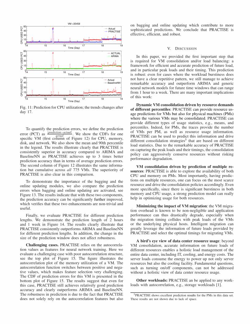
While the results presented before show cases of consistentperiodicity across time, in Figure 11 we show a more challeng-ing case where the trends of the periodical pattern change.The results show that PRACTISE can effectively capture thisthanks to the online updating component. ARIMA can alsoreact to the trend change, but it fails to capture most peakstates. However, BaselineNN can only predict events that havebeen observed before, and are therefore unable to capture suchtrend changes. The experiments cover a variety of data centerconfigurations and applications with various usage patterns,but due to the interest of space, we skip other results here.

14 15 16 17 18 190

15

30

45

60

Time (Day)

CP

U U

SE

D P

CT

VM =35458

Actual

PRACTISE

14 15 16 17 18 190

15

30

45

60

Time (Day)

CP

U U

SE

D P

CT

ACTUAL

ARIMA

14 15 16 17 18 190

15

30

45

60

Time (Day)

CP

U U

SE

D P

CT

Actual

BaselineNN

Fig. 11: Prediction for CPU utilization; the trends changes afterday 17.

To quantify the prediction errors, we define the prediction

error (PCT) as|prediction−actual|

actual. We show the CDFs for one

specific VM (first column of Figure 12) for CPU, memory,disk, and network. We also show the mean and 90th percentilein the legend. The results illustrate clearly that PRACTISE isconsistently superior in accuracy compared to ARIMA andBaselineNN as PRACTISE achieves up to 3 times betterprediction accuracy than in terms of average prediction errors.The second column of Figure 12 illustrates the same informa-tion but cumulative across all 775 VMs. The superiority ofPRACTISE is also clear in this comparison.

To demonstrate the importance of the bagging and theonline updating modules, we also compare the predictionerrors when bagging and online updating are activated, seeFigure 13. The results indicate that with these two components,the prediction accuracy can be significantly further improved,which verifies that these two enhancements are non-trivial anduseful.

Finally, we evaluate PRACTISE for different predictionlengths. We demonstrate the prediction length of 2 hoursand 1 week in Figure 14. The results clearly illustrate thatPRACTISE consistently outperforms ARIMA and BaselineNNfor different prediction lengths. In addition, the change in thesize of the prediction window does not affect robustness.

Challenging cases. PRACTISE relies on the autocorrela-tion values as features for neural network training. Here weevaluate a challenging case with poor autocorrelation structure,see the top plot of Figure 15. The figure illustrates theautocorrelation plot of the memory utilization of a VM. Theautocorrelation function switches between positive and nega-tive values, which makes feature selection very challenging.The CDF of prediction errors for this VM is presented in thebottom plot of Figure 15. The results suggest that even forthis case, PRACTISE still achieves relatively good predictionaccuracy and clearly outperforms ARIMA and BaselineNN.The robustness in prediction is due to the fact that PRACTISEdoes not solely rely on the autocorrelation features but also

on bagging and online updating which contribute to moresophisticated predictions. We conclude that PRACTISE iseffective, efficient, and robust.

V. DISCUSSION

In this paper, we provided the first important step thatis required for VM consolidation and/or load balancing: aframework for efficient and accurate prediction of future load,and in particular peak loads and their timing. This predictionis robust: even for cases where the workload burstiness doesnot have a clear repetitive pattern, we still manage to achieveremarkable accuracy and outperform ARIMA and genericneural network models for future time windows that can rangefrom 1 hour to a week. There are many important implicationsof this work:

Dynamic VM consolidation driven by resource demandsof different percentiles: PRACTISE can provide resource us-age predictions for VMs but also for physical machines (PMs)where the various VMs may be consolidated. PRACTISE canprovide different types of usage statistics, e.g., means, andpercentiles. Indeed, for PMs, the traces provide the numberof VMs per PM, as well as resource usage information.PRACTISE can be used to predict this information and drivedifferent consolidation strategies5 that are based on differentload statistics. Due to the remarkable accuracy of PRACTISEon capturing the peak loads and their timings, the consolidationpolicy can aggressively conserve resources without riskingperformance degradation.

VM consolidation driven by prediction of multiple re-sources: PRACTISE is able to explore the availability of bothCPU and memory on PMs. Most importantly, having predic-tions on multiple resources, one can focus on the most scarceresource and drive the consolidation policies accordingly. Evenmore specifically, since there is significant burstiness in bothmemory and CPU usage, a strong prediction model can reallyhelp in optimizing usage for both resources.

Minimizing the impact of VM migration: the VM migra-tion overhead is known to be non-negligible and applicationperformance can thus drastically degrade, especially whenthe migration timing collides with peak loads of the VMsor the underlying physical hosts. Intelligent migration cangreatly leverage the information of future loads provided byPRACTISE and select the optimal timings for migrating VMs.

A bird’s eye view of data center resource usage: beyondVM consolidation, accurate information on future loads ofdifferent resources enables a holistic load management of theentire data center, including IT, cooling, and energy costs. Theserver loads consume the energy to power up not only serverresources but also the cooling facility. Fundamental questions,such as turning on/off components, can not be addressedwithout a holistic view of data center resource usage.

Other workloads: PRACTISE an be applied to any work-loads with autocorrelation, e.g., storage workloads [1].

5PRACTISE shows excellent prediction results for the PMs in this data set.These results are not shown due to lack of space.

0 50 100 150 2000

0.2

0.4

0.6

0.8

1

CD

F

Absolute PCT Error (%)

VM =33222, CPU USED PCT

ARIMA: Mean =32.4, 90% =135.9

BaselineNN: Mean =29.3, 90% =120.4PRACTISE: Mean =9.3, 90% =18.3

0 50 100 150 2000

0.2

0.4

0.6

0.8

1

CD

F


VM CPU USED PCT

ARIMA: Mean =43.6, 90% =60.2


0 20 40 60 80 1000

0.2

0.4

0.6

0.8

1

CD

F


VM =3788, MEM USED PCT

ARIMA: Mean =17.9, 90% =45.1


0 20 40 60 80 1000

0.2

0.4

0.6

0.8

1

CD

F


VM MEM USED PCT

ARIMA: Mean =21.4, 90% =48.8


0 2 4 60

0.2

0.4

0.6

0.8

1

CD

F


VM =28995, DISK USED PCT

ARIMA: Mean =1.9, 90% =5.3

BaselineNN: Mean =2.1, 90% =4PRACTISE: Mean =0.6, 90% =0.8

0 2 4 60

0.2

0.4

0.6

0.8

1

CD

F


VM DISK USED PCT

ARIMA: Mean =0.9, 90% =2.3


0 100 200 3000

0.2

0.4

0.6

0.8

1

CD

F


VM =3751, NET RX+TX MBPS

ARIMA: Mean =85.8, 90% =253

BaselineNN: Mean =52.7, 90% =149PRACTISE: Mean =27.5, 90% =79.5

0 100 200 3000

0.2

0.4

0.6

0.8

1

CD

F


VM NET RX+TX MBPS

ARIMA: Mean =66.7, 90% =269.5


Fig. 12: Prediction error comparison for different prediction methods. The graphs are for VM CPU utilization (row 1), VMmemory utilization (row 2), VM disk space usage (row 3), VM network bandwidth prediction (row 4). The first column is fora selected VM and the second column shows accumulated results over all VMs. Prediction length is 1 day ahead.

VI. RELATED WORK

ARMA/ARIMA [11] have been widely used for time seriesprediction in several systems areas. Tran and Reed use ARIMAto improve block prefetching for scientific applications [26].They use ARIMA to predict the temporal access pattern andMarkov models to identify spatial access patterns and manageto identify what and how much to prefetch. Their predictoris implemented on the Linux file system. In [5] ARIMA isused for effective user traffic prediction for capacity planning.The authors focus on cost-efficient database replication thatis driven by the anticipated user traffic within the LinkedIn

social network. ARIMA models have also been used in sensornetworks to reduce the frequency of sampling and to improveon energy efficiency by transmitting only deviations fromthe ARIMA-predicted values [27]. Anomaly detection is yetanother area where ARIMA models have been used [28].

Machine learning techniques are used to overcome thelimitation of the linear basis function of ARIMA models andare used for effective characterization of TCP/IP [29] and webserver views [30]. Neural networks are used for performanceprediction of the total order broadcast, which is a key buildingblock for fault-tolerant replicated systems [31]. Ensembles of

0 5 10 15 20 25 300

0.2

0.4

0.6

0.8

1

CD

F



NoBagging: Mean =7.6, 90% =25.2

Bagging: Mean =2.4, 90% =5.9

0 20 40 60 800

0.2

0.4

0.6

0.8

1

CD

F



NoUpdate: Mean =28, 90% =62.4

OnlineUpdate: Mean =17.7, 90% =58.1

Fig. 13: Prediction error comparison of VM CPU utilizationwith and without bagging (top plot), and with and withoutonline updating module (bottom plot).

0 50 100 150 2000

0.2

0.4

0.6

0.8

1

CD

F


VM CPU USED PCT

ARIMA: Mean =22.4, 90% =40.7


0 50 100 150 2000

0.2

0.4

0.6

0.8

1

CD

F


VM CPU USED PCT

ARIMA: Mean =34.4, 90% =113.6


Fig. 14: Prediction error comparison of VM CPU utilizationfor prediction length of 2 hours (top plot) and 1 week (bottomplot). The results are accumulated across all VMs.

time neural network models have been used to project diskutilization trends in a cloud setting [32]. Neural networks andhidden Markov models are used for automatic IO pattern clas-sification and are evaluated with both sequential and parallelbenchmarks [21]. Probabilistic models that define workloadstates via Markov Modulated Poisson Processes have beenused in [1] to interleave workloads with different performanceobjectives. Machine learning techniques have been widely usedfor workload prediction [33], [34], [35], [36]. In contrast tothese works, we rely on the autocorrelation and automate the

0 3 6 9 12 15 18 21 24 27 30 33 36 39 42 45−0.25

0

0.25

0.5

0.75

1VM =34726

Time (Day)

AC

F

0 20 40 60 80 1000

0.2

0.4

0.6

0.8

1

CD

F


VM =34726, MEM USED PCT

ARIMA: Mean =49.5, 90% =69.4

BaselineNN: Mean =56.6, 90% =125.3

PRACTISE: Mean =27.5, 90% =49.8

Fig. 15: A challenging case (VM 34726). Autocorrelation (topplot) and prediction error comparison (bottom plot) of memoryutilization for different prediction methods.

entire learning process.

The effectiveness of the proposed neural network approachthat we advocate in this paper is based on statistical analysis ofthe workload so that the most relevant features are selected forthe training data set. Training the model with careful featureselection significantly improves its accuracy and stability butalso increases the speed of training and prediction, makingit appropriate to use for online performance prediction andcapacity planning. In addition, due to the appropriate featureselection, PRACTISE can provide short-term (e.g., 15 minutes)to long-term (e.g., one day or one week ahead) predictionsand achieve excellent accuracy. These superior predictionsfacilitate robust long-term capacity planning and resourceallocation.

VII. CONCLUSION AND FUTURE WORK

In this paper, we develop PRACTISE, an enhanced neuralnetwork based framework for predicting the usage of variousresources in data centers. PRACTISE uses autocorrelation-based feature selection, boostrap aggregation, and online up-dating. We extensively evaluate PRACTISE on predictingCPU, memory, disk and network usage on a set of 775VMs over a period of 2 months and compare its predictioneffectiveness to ARIMA and basic neural network models. Weare able to achieve up to 3 times better prediction accuracy interms of average prediction errors and dramatic improvements(2- to 9-fold) with respect to the prediction timings. Thanksto the excellent prediction accuracy of PRACTISE, we areable to efficiently capture the peak loads in terms of theirintensities and timing, in contrast to classic time series models.In our future work we intend to use PRACTISE to explore VMconsolidation and migration policies tailored to cater to peakdemands in a cost-effective way.

VIII. ACKNOWLEDGMENTS

This work is supported by NSF grant CCF-1218758 andEU commission FP7 GENiC project (Grant Agreement No608826).

REFERENCES

[1] J. Xue, F. Yan, A. Riska, and E. Smirni, “Storage workload isolationvia tier warming: How models can help,” in Proceedings of the 11th

ICAC, 2014, pp. 1–11.

[2] Y. Zhang, G. Soundararajan, M. W. Storer, L. N. Bairavasundaram,S. Subbiah, A. C. Arpaci-Dusseau, and R. H. Arpaci-Dusseau, “Warm-ing up storage-level caches with Bonfire,” in FAST, 2013, pp. 59–72.

[3] H. Herodotou, H. Lim, G. Luo, N. Borisov, L. Dong, F. B. Cetin, andS. Babu, “Starfish: a self-tuning system for big data analytics.” in CIDR,vol. 11, 2011, pp. 261–272.

[4] J. Cohen, B. Dolan, M. Dunlap, J. M. Hellerstein, and C. Welton, “Madskills: new analysis practices for big data,” Proceedings of the VLDB

Endowment, vol. 2, no. 2, pp. 1481–1492, 2009.

[5] Z. Zhuang, H. Ramachandra, C. Tran, S. Subramaniam, C. Botev,C. Xiong, and B. Sridharan, “Capacity planning and headroom analysisfor taming database replication latency: experiences with linkedininternet traffic,” in Proceedings of the 6th ACM/SPEC ICPE, 2015,pp. 39–50.

[6] C. Clark, K. Fraser, S. Hand, J. G. Hansen, E. Jul, C. Limpach,I. Pratt, and A. Warfield, “Live migration of virtual machines,” in NSDI.USENIX Association, 2005, pp. 273–286.

[7] M. Nelson, B.-H. Lim, G. Hutchins et al., “Fast transparent migrationfor virtual machines.” in USENIX ATC, 2005, pp. 391–394.

[8] T. Wood, P. J. Shenoy, A. Venkataramani, and M. S. Yousif, “Black-boxand gray-box strategies for virtual machine migration.” in NSDI, vol. 7,2007, pp. 17–17.

[9] R. Birke, A. Podzimek, L. Y. Chen, and E. Smirni, “State-of-the-practicein data center virtualization: Toward a better understanding of VMusage,” in DSN, 2013, pp. 1–12.

[10] R. Birke, M. Björkqvist, L. Y. Chen, E. Smirni, and T. Engbersen,“(big)data in a virtualized world: volume, velocity, and variety in clouddatacenters,” in FAST, 2014, pp. 177–189.

[11] B. George, Time Series Analysis: Forecasting & Control, 3rd ed.Pearson Education India, 1994.

[12] L. Breiman, “Bagging predictors,” Machine learning, vol. 24, no. 2, pp.123–140, 1996.

[13] L. M. Leemis and S. K. Park, Discrete-event simulation: a first course.Pearson Prentice Hall Upper Saddle River, NJ, 2006.

[14] P. Goodwin, “The holt-winters approach to exponential smoothing: 50years old and going strong,” Foresight, pp. 30–34, 2010.

[15] R. J. Frank, N. Davey, and S. P. Hunt, “Time series prediction andneural networks,” Journal of Intelligent and Robotic Systems, vol. 31,no. 1-3, pp. 91–103, 2001.

[16] H. Demuth, M. Beale, and M. Hagan, “Neural network toolboxT M 6,”User′s Guide, 2008.

[17] M. H. Hassoun, Fundamentals of Artificial Neural Networks, 1st ed.Cambridge, MA, USA: MIT Press, 1995.

[18] T. Hill, M. O’Connor, and W. Remus, “Neural network models for timeseries forecasts,” Management Science, vol. 42, no. 7, pp. 1082–1092,1996.

[19] G. Upton and I. Cook, A Dictionary of Statistics 3e. Oxford universitypress, 2014.

[20] M. L. Marx and R. J. Larsen, Introduction to mathematical statistics

and its applications. Pearson/Prentice Hall, 2006.

[21] T. M. Madhyastha and D. A. Reed, “Learning to classify parallelinput/output access patterns,” IEEE Trans. Parallel Distrib. Syst.,vol. 13, no. 8, pp. 802–813, 2002. [Online]. Available: http://doi.ieeecomputersociety.org/10.1109/TPDS.2002.1028437

[22] A. K. Maji, S. Mitra, B. Zhou, S. Bagchi, and A. Verma, “Mitigat-ing interference in cloud services by middleware reconfiguration,” inProceedings of the 15th International Middleware Conference. ACM,2014, pp. 277–288.

[23] J. S. Chase, D. C. Anderson, P. N. Thakar, A. M. Vahdat, and R. P.Doyle, “Managing energy and server resources in hosting centers,” inACM SIGOPS Operating Systems Review, vol. 35, no. 5. ACM, 2001,pp. 103–116.

[24] X. Zhu, D. Young, B. J. Watson, Z. Wang, J. Rolia, S. Singhal,B. McKee, C. Hyser, D. Gmach, R. Gardner et al., “1000 islands:

Integrated capacity and workload management for the next generationdata center,” in Autonomic Computing, 2008. ICAC’08. International

Conference on. IEEE, 2008, pp. 172–181.

[25] P. Xiong, C. Pu, X. Zhu, and R. Griffith, “vperfguard: an automatedmodel-driven framework for application performance diagnosis in con-solidated cloud environments,” in Proceedings of the 4th ACM/SPEC

International Conference on Performance Engineering. ACM, 2013,pp. 271–282.

[26] N. Tran and D. A. Reed, “Automatic ARIMA time seriesmodeling for adaptive I/O prefetching,” IEEE Trans. Parallel Distrib.

Syst., vol. 15, no. 4, pp. 362–377, 2004. [Online]. Available:http://doi.ieeecomputersociety.org/10.1109/TPDS.2004.1271185

[27] M. Li, D. Ganesan, and P. J. Shenoy, “PRESTO: feedback-driven data management in sensor networks,” IEEE/ACM Trans.

Netw., vol. 17, no. 4, pp. 1256–1269, 2009. [Online]. Available:http://doi.acm.org/10.1145/1618562.1618581

[28] B. Zhu and S. Sastry, “Revisit dynamic ARIMA based anomalydetection,” in PASSAT/SocialCom 2011, Privacy, Security, Risk and

Trust (PASSAT), 2011 IEEE Third International Conference on and

2011 IEEE Third International Conference on Social Computing

(SocialCom), Boston, MA, USA, 9-11 Oct., 2011, 2011, pp. 1263–1268. [Online]. Available: http://doi.ieeecomputersociety.org/10.1109/PASSAT/SocialCom.2011.84

[29] P. Cortez, M. Rio, M. Rocha, and P. Sousa, “Multi-scale internet trafficforecasting using neural networks and time series methods,” Expert

Systems, vol. 29, no. 2, pp. 143–155, 2012.

[30] J. Li and A. W. Moore, “Forecasting web page views: methods andobservations,” Journal of Machine Learning Research, vol. 9, no. 10,pp. 2217–2250, 2008.

[31] M. Couceiro, P. Romano, and L. Rodrigues, “A machine learningapproach to performance prediction of total order broadcast protocols,”in 4th IEEE SASO, 2010, pp. 184–193.

[32] M. Stokely, A. Mehrabian, C. Albrecht, F. Labelle, and A. Merchant,“Projecting disk usage based on historical trends in a cloud environ-ment,” in Proceedings of the 3rd workshop on ScienceCloud, 2012, pp.63–70.

[33] N. K. Ahmed, A. F. Atiya, N. E. Gayar, and H. El-Shishiny, “Anempirical comparison of machine learning models for time seriesforecasting,” Econometric Reviews, vol. 29, no. 5-6, pp. 594–621, 2010.

[34] L. M. Saini and M. K. Soni, “Artificial neural network-based peak loadforecasting using conjugate gradient methods,” Power Systems, IEEE

Transactions on, vol. 17, no. 3, pp. 907–912, 2002.

[35] S. F. Crone, M. Hibon, and K. Nikolopoulos, “Advances in forecastingwith neural networks? empirical evidence from the nn3 competition ontime series prediction,” International Journal of Forecasting, vol. 27,no. 3, pp. 635–660, 2011.

[36] K.-L. Ho, Y.-Y. Hsu, and C.-C. Yang, “Short term load forecasting usinga multilayer neural network with an adaptive learning algorithm,” Power

Systems, IEEE Transactions on, vol. 7, no. 1, pp. 141–149, 1992.

practise: robust prediction of data center time series

Documents