practical meteorology: an algebra-based survey of ... · practical meteorology: an algebra-based...
TRANSCRIPT
219
Copyright © 2017 by Roland Stull. Practical Meteorology: An Algebra-based Survey of Atmospheric Science. v1.02b
8 SATELLITES & RADAR
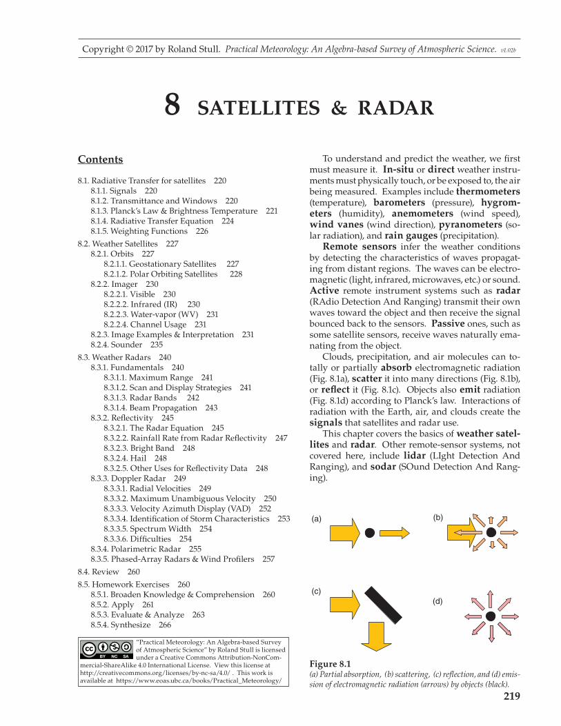
To understand and predict the weather, we first must measure it. In-situ or direct weather instru-ments must physically touch, or be exposed to, the air being measured. Examples include thermometers (temperature), barometers (pressure), hygrom-eters (humidity), anemometers (wind speed), wind vanes (wind direction), pyranometers (so-lar radiation), and rain gauges (precipitation). Remote sensors infer the weather conditions by detecting the characteristics of waves propagat-ing from distant regions. The waves can be electro-magnetic (light, infrared, microwaves, etc.) or sound. Active remote instrument systems such as radar (RAdio Detection And Ranging) transmit their own waves toward the object and then receive the signal bounced back to the sensors. Passive ones, such as some satellite sensors, receive waves naturally ema-nating from the object. Clouds, precipitation, and air molecules can to-tally or partially absorb electromagnetic radiation (Fig. 8.1a), scatter it into many directions (Fig. 8.1b), or reflect it (Fig. 8.1c). Objects also emit radiation (Fig. 8.1d) according to Planck’s law. Interactions of radiation with the Earth, air, and clouds create the signals that satellites and radar use. This chapter covers the basics of weather satel-lites and radar. Other remote-sensor systems, not covered here, include lidar (LIght Detection And Ranging), and sodar (SOund Detection And Rang-ing).
Contents
8.1. Radiative Transfer for satellites 2208.1.1. Signals 2208.1.2. Transmittance and Windows 2208.1.3. Planck’s Law & Brightness Temperature 2218.1.4. Radiative Transfer Equation 2248.1.5. Weighting Functions 226
8.2. Weather Satellites 2278.2.1. Orbits 227
8.2.1.1. Geostationary Satellites 2278.2.1.2. Polar Orbiting Satellites 228
8.2.2. Imager 2308.2.2.1. Visible 2308.2.2.2. Infrared (IR) 2308.2.2.3. Water-vapor (WV) 2318.2.2.4. Channel Usage 231
8.2.3. Image Examples & Interpretation 2318.2.4. Sounder 235
8.3. Weather Radars 2408.3.1. Fundamentals 240
8.3.1.1. Maximum Range 2418.3.1.2. Scan and Display Strategies 2418.3.1.3. Radar Bands 2428.3.1.4. Beam Propagation 243
8.3.2. Reflectivity 2458.3.2.1. The Radar Equation 2458.3.2.2. Rainfall Rate from Radar Reflectivity 2478.3.2.3. Bright Band 2488.3.2.4. Hail 2488.3.2.5. Other Uses for Reflectivity Data 248
8.3.3. Doppler Radar 2498.3.3.1. Radial Velocities 2498.3.3.2. Maximum Unambiguous Velocity 2508.3.3.3. Velocity Azimuth Display (VAD) 2528.3.3.4. Identification of Storm Characteristics 2538.3.3.5. Spectrum Width 2548.3.3.6. Difficulties 254
8.3.4. Polarimetric Radar 2558.3.5. Phased-Array Radars & Wind Profilers 257
8.4. Review 260
8.5. Homework Exercises 2608.5.1. Broaden Knowledge & Comprehension 2608.5.2. Apply 2618.5.3. Evaluate & Analyze 2638.5.4. Synthesize 266
Figure 8.1(a) Partial absorption, (b) scattering, (c) reflection, and (d) emis-sion of electromagnetic radiation (arrows) by objects (black).
(a) (b)
(c)(d)
“Practical Meteorology: An Algebra-based Survey of Atmospheric Science” by Roland Stull is licensed under a Creative Commons Attribution-NonCom-
mercial-ShareAlike 4.0 International License. View this license at http://creativecommons.org/licenses/by-nc-sa/4.0/ . This work is available at https://www.eoas.ubc.ca/books/Practical_Meteorology/

220 CHAPTER8•SATELLITES&RADAR
8.1. RADIATIVE TRANSFER FOR SATELLITES
8.1.1. Signals Weather satellites have passive sensors called radiometers that measure upwelling electromag-netic radiation from the Earth and atmosphere. In-frared (IR, long-wave) and microwave radiation are emitted by the Earth, ocean, atmosphere, clouds, and the sun (see the Radiation chapter). Visible light (short-wave or solar radiation) is emitted by the sun and reflected and absorbed by the Earth sys-tem. Additional portions of the electromagnetic spectrum are useful for remote sensing. What the satellite can “see” in any one wave-length depends on the transparency of the air at that wavelength. A perfectly transparent atmosphere al-lows the upwelling radiation from the Earth’s sur-face or highest cloud top to reach the satellite. Thus, wavelengths for which the air is transparent (Fig. 8.2a) are good for observing clouds and land use. If air molecules strongly absorb upwelling radia-tion at another wavelength, then none of the signal at that wavelength from the Earth and clouds will reach the satellite (i.e., an opaque atmosphere). But according to Kirchhoff’s law (see the Radiation chap-ter), absorptivity equals the emissivity at that wave-length. This atmosphere will emit its own spectrum of radiation according to Planck’s law, causing the atmosphere to glow like an infrared light bulb (Fig. 8.2b). Wavelengths with this characteristic are good for observing the top of the atmosphere, but are bad for remote sensing of the Earth and clouds. For other wavelengths, the atmosphere partially absorbs the upwelling radiation, causing the Earth and clouds to look dimmer (Fig. 8.2c). But this usu-ally never happens alone, because Kirchhoff’s law says that the atmosphere will also partially emit in the same wavelengths. The result is a dim view of the Earth, partially masked by a dimly glowing at-mosphere (Fig. 8.2d). For wavelengths scattered by air molecules, the signal from the Earth and clouds becomes blurred (Fig. 8.2e). For some wavelengths, this blurring is so extreme that no useful signal reaches the satel-lite, other than noise from all the scattered light rays. Finally, there are other wavelengths where all of the processes happen: atmospheric scattering, absorp-tion, and emission (Fig. 8.2f).
8.1.2. Transmittance and Windows Of the electromagnetic energy that is upwelling through any height, the percentage of it that comes out the top of the atmosphere is called transmit-tance. Transmittance varies with wavelength.
Figure 8.2Illustration of visibility of the Earth and atmosphere as viewed by satellite. Figure (d) is overly simplistic, because variations in atmospheric constituents in the mid and upper atmosphere will cause atmospheric emissions (glowing) to be uneven.
(a) transparentatmosphere
(b) opaque, emittingatmosphere
(c) partially absorbingatmosphere
(e) transparent, scattering atmosphere
(d) partially emitting &absorbing atmosphere
(f) emitting, absorbing, &scattering atmosphere
R. Stull
Figure 8.3Windows in the electromagnetic spectrum.
0%
20%
40%
60%
80%
100%
Tran
smitt
ance
window
dirtywindow
shou
lder
Wavelength

R.STULL•PRACTICALMETEOROLOGY 221
Portions of the spectrum where transmittances are large are called windows (Fig. 8.3), by analo-gy to visible light passing through clear glass win-dows. At wavelengths near the window, there can be shoulder regions where transmittance rapidly changes. Portions of the spectrum having partial transmittance are sometimes called dirty win-dows. By designing satellite-borne radiometers that are sensitive to different window and non-window wavelengths, you can measure different characteris-tics of the Earth and atmosphere. Figures 8.4a-d (next 2 pages) show the transmit-tance at different wavelengths. Different gases in the atmosphere have different molecular vibration and rotation modes, causing them to absorb at dis-crete wavelengths called absorption lines. In Fig. 8.4, the windows are regions with transmittance of about 80% or higher. These transmittance curves are not physical laws and are not constant, but can change slightly with at-mospheric conditions. The absorption bands (i.e., non-window regions) shift wavelength very slightly with temperature and pressure. The amount of absorption and transmission de-pend strongly on the concentration of absorbing gas along the path length of the radiation (see Beer’s Law in the Radiation chapter). Some gas concentra-tions vary with season (carbon dioxide CO2), some vary hourly depending on the weather (water vapor H2O, ozone O3), while others are relatively constant. Additional gases indicated in these figures are mo-lecular oxygen (O2), methane (CH4), carbon monox-ide (CO), and nitrous oxide (N2O). Water vapor is a major absorber, so more humid conditions and deeper moist layers cause greater absorption. Recall from Chapter 1 that most of our storms and most of the atmosphere’s humidity are trapped within the troposphere. Thus, transmit-tance of surface emissions is weakest in the tropics (high humidity and deep troposphere) and stron-gest near the poles (low absolute humidity and shal-low troposphere). At mid latitudes, transmittance is greatest in winter (low humidity, shallow tropo-sphere) and weakest in summer (higher humidity and deeper troposphere). Transmittance can easily vary by plus or minus 20% between these different locations and seasons in some portions of the spec-trum, especially for wavelengths greater than 5 µm. Another factor that reduces transmittance is scattering by air molecules and aerosols (e.g., air-pollution particles). Scattering increases (causing transmittance to decrease) as wavelength gets short-er (dashed curve in Fig. 8.4a). For cleaner air, the dashed curve is higher and transmittance is greater, but the opposite occurs for heavily polluted, aerosol-laden air. The visible light portion of the spectrum
is a dirty window region. Fig. 8.4 shows that the atmosphere is clearer in some of the IR windows than in the visible light portion of the spectrum that you see every day with your eyes. So far, we have examined atmospheric transmit-tance (the left column of images in Fig. 8.2). Next, we look at atmospheric emissions (right column of Fig. 8.2).
8.1.3. Planck’s Law & Brightness Temperature In the Radiation chapter, Planck’s law allowed computation of total energy flux radiating from a blackbody object per unit wavelength (W·m–2·µm–1) as a function of temperature. Emissions from a flat surface are in all directions, illuminating a hemi-sphere around the object. But a satellite cannot measure the total radiation coming out of the Earth or atmosphere — it can mea-sure only the portion of radiation that happens to be coming toward the satellite within the solid angle intercepted by the radiometer. Assuming the radia-tion is uniform in all directions (i.e., isotropic), then the portion of radiative flux per unit wavelength λ per unit steradian (sr) of solid angle is Planck’s Law equation divided by π:
B Tc
cT
Bλ
λ
λ
( )·
exp·
=
−
−1
5
2 1 •(8.1)
where B is the blackbody radiance in units ofW·m–2·µm–1·sr–1, and
c1B = 1.191 042 82 x 108 W·m–2·µm4·sr–1
c2 = 1.438 775 2 x 104 µm·K .
Thus, c1B = c1/π , where c1 was from eq. (2.13). Don’t forget that T must be in units of Kelvin. A steradian is the solid angle with vertex at the center of a sphere
Sample Application Wavelength 1.85 µm has: (a) what transmittance, and (b) corresponds to which sketch in Fig. 8.2 of Earth visibility as viewed from space?
Find the AnswerGiven: λ = 1.85 µmFind: (a) transmittance = ? % , (b) Earth visibility = ?
(a) From Fig. 8.4b, transmittance = 10% approx., mostly due to strong absorption by water vapor.(b) It would look like Fig. 8.2b in the infrared.
Check: (no easy check for this)Exposition: Most water vapor is in the troposphere. Satellites would see it glow like an IR light bulb.

222 CHAPTER8•SATELLITES&RADAR
Figure 8.4 (this page and next)Atmospheric transmittance of upwelling electromagnetic radiation from the Earth’s surface. Wavelength bands: (a) 0 to 1.4 µm; (b) 0 to 6 µm; (c) 5 to 30 µm; and (d) 30 µm to 100 cm (logarithmic scale). For regions of strong absorption (i.e., low transmittance) the dominant absorbing chemical is given. The names and wavelength ranges (shaded boxes) of the spectral bands and satellite radiom-eter channels are indicated. The Advanced Baseline Imager (ABI) on GOES-16 satellites provides both imaging and sounding functions.
Fig.8.4a.
Fig.8.4b.
0%
20%
40%
60%
80%
100%
Tran
smitt
ance
0 0.2 0.4 0.6 0.8 1.0 1.2 1.4
Wavelength (µm)
visible lightredviolet
near uv farultraviolet (uv) C B A
infrared (IR)
GOES-16 ABI channels:
near
molecular scattering
0 0.2 0.4 0.6 0.8 1.0 1.2 1.4
O3 O2
H2O H2O H2OH2O
H2O
H2O
H2O
γ, xrays
GOES-15 sounder channels: 19
Wavelength (µm)
1 2 GLM 3 4GOES-15 imager channels: 1 “visible”
0%
20%
40%
60%
80%
100%
Tran
smitt
ance
Wavelength (µm)
near infrared (IR)vis.uv
GOES-16 ABI:
GOES-15 sounder: 18 1315
0 1 2 3 4 5 6
0 1 2 3 4 5 6
H2O
H2O
CO2
COCH4CO2
H2OH2OH2O
N2O
Wavelength (µm)
many absorption lines (not to scale)
1 2 3 4 5 6 7 8GOES-15 imager: 1 “visible” 2 3“wv”
19

R.STULL•PRACTICALMETEOROLOGY 223
Fig.8.4c.
Fig.8.4d.
Figure 8.4 (continuation)See Chapter 2 for wavelengths emitted by sun and Earth. Upwelling radiation can be either terrestrial radiation emitted from the atmosphere, ocean and the Earth’s surface, or solar radiation reflected upward from the Earth’s surface and from within the atmo-sphere. The Geostationary Lightning Mapper (GLM) has an optical transient sensor sensitive to atomic oxygen emissions at 0.7774 µm — effective both day and night (Fig. 8.4a). Note the wavelength unit changes in Fig. 8.4d.
0%
20%
40%
60%
80%
100%
Tran
smitt
ance
5 10 15 20 25 30Wavelength (µm)
Infrared (IR)Imagers: GOES-16: GOES-15:
GOES-15sounder:
191012
5 10 15 20 25 30
67 5 24 38
O3 CO2CH4H2O H2O
N2O
H2O
Wavelength (µm)
983 “wv” “IR” 4 5
10 11 12 13 14 15 16
0%
20%
40%
60%
80%
100%
Tran
smitt
ance
Wavelength (cm)
Far Infrared (IR)
1001010.10.010.003
Microwave
10 cm1 cm0.1 cm
Radar Bands: Ku X C S L PKa
30 µm 100 µm
O2
O2
H2O
H2O
H2OH2O
Wavelength
100 cm

224 CHAPTER8•SATELLITES&RADAR
(of radius r) that encompasses an area of r2 on the surface of the sphere; 4π sr cover the whole surface. Fig. 8.5 shows Planck’s law plotted differently; namely, blackbody radiance vs. temperature. Black-body radiance increases monotonically with in-creasing temperature. Hotter objects emit greater radiation (assuming a blackbody emissivity of 1.0). You can also use Planck’s law in reverse. Plug a measured radiance Lλ into eq. (8.1) in place of Bλ, and solve for temperature. This temperature is called the brightness temperature (TB), which is the temperature of a hypothetical blackbody that produces the same radiance as the measured radi-ance: = λ
+ λ
−
λ
/
ln 1·
2
15
Tc
cL
BB
•(8.2)
8.1.4. Radiative Transfer Equation Recall from Fig. 8.2 that surface emissions might be partially or totally absorbed by the atmosphere before reaching the satellite. The atmosphere emits its own radiation, some of which might also be lost by absorption before reaching the satellite. These effects are summarized by the radiative transfer equation:
L B T e z B Tskin sfc j j jj
λ λ λ λ λ λτ τ= +=
( )·ˆ ( )· ( )·ˆ, ,1
nn
∑ (8.3)
where Lλ is the radiance at wavelength λ that ex-its the top of the atmosphere and can be observed by satellite. Tskin is the temperature of the top few molecules of the Earth’s surface, NOT the standard meteorological “surface” temperature measured 2 m above ground. τ̂ is transmittance; e is emissivity. This equation is called Schwarzchild’s eq.
Sample Application What is the blackbody radiance at wavelength 10.9 µm from a cloud top of temperature –20°C ?
Find the AnswerGiven: T = –20°C = 253 K, λ = 10.9 µmFind: Bλ(T) = ? W·m–2·µm–1·sr–1
Use eq. (8.1):
B Tλ ( )
exp
= (1.191x10 W·m µm sr )·(10.9µm)8 –2 4 –1 –5
11.44x10 µm·K(10.9µm)·(253K)
4
− 11
= 4.22 W·m–2·µm–1·sr–1
Check: Units OK. Physics OK.Exposition: 10.9 µm is an IR wavelength in an at-mospheric window region of the spectrum (Fig. 8.4). Thus, these emissions from the cloud would be ab-sorbed very little by the intervening atmosphere, and could be observed by satellite. That is why the “IR” satellite channels are in that spectral band.
Sample Application A satellite measures a radiance of 1.1 W·m–2·µm–1 ·sr–1 at wavelength 6.7 µm. What is the brightness temperature?
Find the AnswerGiven: Lλ(T)= 1.1 W·m–2·µm–1·sr–1, λ = 6.7 µmFind: TB = ? K
Use eq. (8.2) :
TB =
+−
(1.44x10 µm·K) µm
1.191x10 W m
4
8 2/( . )
ln·
6 7
1µµm sr µm
1.1W m µm sr
4 1
2 1 1
− −
− − −
·( . )
·
6 7 5
= 239 K = –34°C
Check: Units OK. Physics OK.Exposition: 6.7 µm is an IR wavelength in a water-va-por absorption (=emission) part of the spectrum (Fig. 8.4). The atmosphere is partly opaque in this region, so the radiation received at the satellite was emitted from the air. This brightness temperature is about –34°C. Such cold temperatures are typically found in the up-per troposphere. Thus, we can infer from the standard atmosphere that this satellite channel is “seeing” the upper troposphere.
Figure 8.5Planck’s law emissions (B) vs. brightness temperature TB. for various wavelengths (λ).
0 100 200 300 400 500
Bλ
(W m
–2
µm
–1
sr –
1 )
λ =15 µm
λ =10 µm
λ =5 µm
λ =2 µm
λ =1 µm λ =
0.5 µm10–25
10–20
10–15
10–10
10–5
100
TB (K)

R.STULL•PRACTICALMETEOROLOGY 225
The first term on the right hand side (RHS) gives the blackbody emissions from the Earth’s surface, re-duced by the overall transmittance τ̂ λ, sfc between the surface and the top of the atmosphere (from Fig. 8.4). Namely, satellites can see the Earth’s surface at wavelengths for which the air is not totally opaque. The second term on the RHS is a sum over all at-mospheric layers ( j = 1 to n), representing the differ-ent heights zj in the atmosphere. The net emissions from any one layer j are equal to the emissivity eλ(zj) of the air at that height for that wavelength times the blackbody emissions. However, the resulting radi-ance is reduced by the transmittance τ̂ λ,j between that height and the top of the atmosphere. Transmittance τ̂ = 0 if all of the radiation is ab-sorbed before reaching the top of the atmosphere. Transmittance = 1 – absorptance; namely, τ̂ =1 – a. To help understand the second term, consider a hypothetical or “toy” profile of transmittance (Fig. 8.6). For the air below 5 km altitude, τ̂ = 0, thus a = (1 – τ̂ ) = 1. But if a = 1, then e = 1 from Kirch-hoff’s Law (see the Radiation chapter). Hence, the layers of air below 5 km are efficient emitters of ra-diation, but none of this radiation reaches the top of the atmosphere because it is all absorbed by other air molecules along the way, as indicated by zero transmissivity. So a satellite cannot “see” the air at this range of heights. Above 10 km altitude, although the atmosphere is transparent in this toy profile, it has zero emissivity. So no radiation is produced from the air at these al-titudes, and again the satellite cannot see this air. But for heights between 5 and 10 km, the atmo-sphere is partially emitting (has nonzero emissivity), and the resulting upwelling radiation is not totally absorbed (as indicated by nonzero transmissivity). Thus, radiation from this layer can reach the satel-lite. The satellite can see through the atmosphere down to this layer, but can’t see air below this layer. Thus, with the right wavelength, satellites can measure brightness temperature at an elevated layer of cloudless air. At other wavelengths with differ-ent transmittance profiles, satellites can measure temperature in different layers, at the top of the at-mosphere, at cloud top, or at the Earth’s surface. In general, heights where transmittance changes are heights for which the air can be remotely ob-served. After a bit of math, the radiative transfer equation can be rewritten in terms of transmittance change ∆ τ̂ = [ τ̂ top of layer j – τ̂ bottom of layer j ]:
L B T B Tskin sfc j j
j
n
λ λ λ λ λτ τ= +=∑( )·ˆ ( )· ˆ, ,∆
1 (8.4)
If the full atmospheric depth is black (i.e., no surface emissions reach outer space), then ∆ =
=∑ τ̂λ,jjn
11 .
Figure 8.6Hypothetical variation of atmospheric transmit-tance ( τ̂ ), absorptance (a), and emittance (e) with height (z).
0
5
10
15
20
z(km)
τ0
01
a01
1
e
ˆ
Sample Application Use the IR transmittance profile of Fig. 8.6, for λ = 6.7 µm. Suppose the vertical temperature profile in the atmosphere is: z (km) T (°C) 15 to 20 –40 10 to 15 –30 5 to 10 –20 0 to 5 0 and the Earth’s surface (skin) temperature is 15°C. Find the upwelling IR radiation at the top of the at-mosphere.
Find the AnswerGiven: the data above.Find: Lλ = ? W·m–2·µm–1·sr–1 .
You can save some work by thinking about the problem first. From Fig. 8.6, the transmittance τ̂ λ,sfc is 0 at the surface (z = 0). Thus, none of the surface emis-sions will reach the top of the atmosphere, so Tskin is irrelevant, and the first term on the RHS of eq. (8.4) is zero. Also, as discussed, the satellite can’t see the layers between 0 to 5 km and 10 to 20 km for this toy profile, so the temperatures in these layers are also irrelevant. Thus, all terms in the sum in eq. (8.4) are zero except the one term for the one layer at 5 to 10 km. In this layer, the absolute temperature is T = 273 – 20°C = 253 K. Across this layer, the change of trans-mittance is ∆ τ̂ = [ 1 – 0 ]. Thus, the only nonzero part of eq. (8.4) is: Lλ = 0 + Bλ(253 K) · [ 1 – 0 ]where you can solve for Bλ using eq. (8.1). Lλ = Bλ(253 K) = 1.82 W·m–2·µm–1·sr–1 .
Check: Units OK. Physics OK.Exposition: A lot of work was saved by thinking first.
20
10
T (°C)
z(km)
–40 –20 00
20
Tskin=15°C
226 CHAPTER8•SATELLITES&RADAR
8.1.5. Weighting Functions In eq. (8.4) the factor ∆ τ̂ within the sum acts as a weight that determines the relative contribution of each layer to the total radiance out the top of the at-mosphere at that wavelength. Use the symbol Wλ,j for these weights (i.e., Wλ,j = ∆ τ̂ λ,j ). With this trivial notation change, the radiative transfer equation is: L B T B T Wskin sfc j j
j
n
λ λ λ λ λτ= +=∑( )·ˆ ( )·, ,
1 •(8.5)
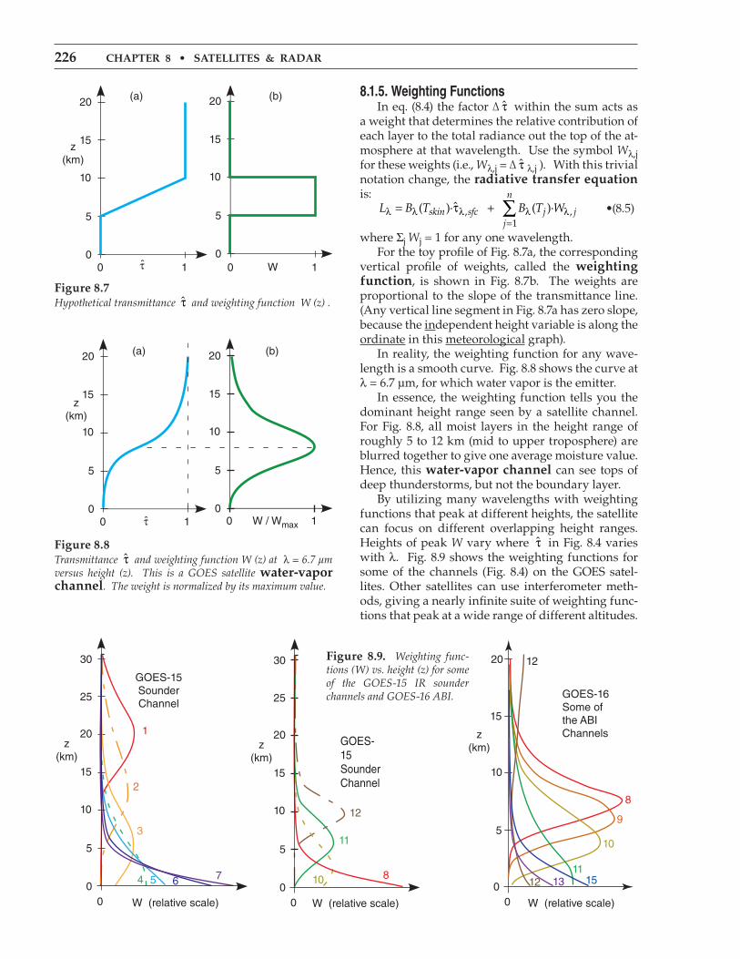
where Σj Wj = 1 for any one wavelength. For the toy profile of Fig. 8.7a, the corresponding vertical profile of weights, called the weighting function, is shown in Fig. 8.7b. The weights are proportional to the slope of the transmittance line. (Any vertical line segment in Fig. 8.7a has zero slope, because the independent height variable is along the ordinate in this meteorological graph). In reality, the weighting function for any wave-length is a smooth curve. Fig. 8.8 shows the curve at λ = 6.7 µm, for which water vapor is the emitter. In essence, the weighting function tells you the dominant height range seen by a satellite channel. For Fig. 8.8, all moist layers in the height range of roughly 5 to 12 km (mid to upper troposphere) are blurred together to give one average moisture value. Hence, this water-vapor channel can see tops of deep thunderstorms, but not the boundary layer. By utilizing many wavelengths with weighting functions that peak at different heights, the satellite can focus on different overlapping height ranges. Heights of peak W vary where τ̂ in Fig. 8.4 varies with λ. Fig. 8.9 shows the weighting functions for some of the channels (Fig. 8.4) on the GOES satel-lites. Other satellites can use interferometer meth-ods, giving a nearly infinite suite of weighting func-tions that peak at a wide range of different altitudes.
Figure 8.9. Weighting func-tions (W) vs. height (z) for some of the GOES-15 IR sounder channels and GOES-16 ABI.
Figure 8.8Transmittance τ̂ and weighting function W (z) at λ = 6.7 µm versus height (z). This is a GOES satellite water-vapor channel. The weight is normalized by its maximum value.
Figure 8.7Hypothetical transmittance τ̂ and weighting function W (z) .
0
5
10
15
20(a) (b)
0
5
10
15
20
z(km)
τ0 1 0 1Wˆ
(a) (b)
0
5
10
15
20
z(km)
0 10
5
10
15
20
0 1W / Wmaxτ̂
00
5
10
15
20
25
30
1
2
3
4 5 6 7
z(km)
W (relative scale)
GOES-15SounderChannel
00
5
10
15
20
GOES-16Some ofthe ABIChannelsz
(km)
W (relative scale)
8
9
10
1115
12
12 13
00
5
10
15
20
25
30
GOES-15SounderChannel
12
11
10 8
z(km)
W (relative scale)

R.STULL•PRACTICALMETEOROLOGY 227
8.2. WEATHER SATELLITES
8.2.1. Orbits Artificial satellites such as weather satellites or-biting the Earth obey the same orbital mechanics as planets orbiting around the sun. For satellites in near-circular orbits, the pull by the Earth’s gravity fG balances centrifugal force fC :
fG M m
RG = · ·
2 •(8.6)
ft
m RCorbit
= π
22
· · •(8.7)
where R is the distance between the center of the Earth and the satellite, m is the mass of the satellite, M is the mass of the Earth (5.9742x1024 kg), and G is the gravitational constant (6.6742x10⁻¹¹ N·m2·kg–2 ). See Appendix B for lists of constants. Solve for the orbital time period torbit by setting fG = fC:
tR
G Morbit =π2 3 2·
·
/
•(8.8)
Orbital period does not depend on satellite mass, but increases as satellite altitude increases. Weather satellite orbits are classified as either polar-orbiting or geostationary (Fig. 8.10). Polar-orbiters are low-Earth-orbit (LEO) satellites.
8.2.1.1.GeostationarySatellites Geostationary satellites are in high Earth orbit over the equator, so that the orbital period matches the Earth’s rotation. Relative to the fixed stars, the Earth rotates 360° in 23.934 469 6 h, which is the du-ration of a sidereal day. With this orbital period, geostationary satellites appear parked over a fixed point on the equator. From this vantage point, the satellite can take a series of photographs of the same location, allowing the photos to be combined into a repeating movie called a satellite loop. Disadvantages of geostationary satellites include the following: distance from Earth is so great that larger magnification is needed to resolve smaller clouds; many satellites must be parked at different longitudes for imagery to cover the globe; imaging might be interrupted during nights near the equi-noxes because the solar panels are eclipsed by the Earth and are in darkness; and polar regions are dif-ficult to see. Satellites have planned lifetimes of about 5 to 17 years, so older satellites must be continually replaced with newer ones. Lifetimes are limited partly because of the limited storage of propellants needed to make orbital corrections. Satellites are
Sample Application At what (a) distance above the Earth’s center, & (b) altitude above the Earth’s surface, must a geostationary satellite be parked to have an orbital period of exactly one sidereal day? Use Appendix B for Earth constants.
Find the AnswerGiven: torbit = 23.934 469 6 h = 86,164 s = sidereal day. M = 5.973 6 x 1024 kg G = 6.674 28 x 10–11 m3·s–2·kg–1 Find: (a) R = ? km, (b) z = ? km
(a) Rearrange eq. (8.8): R = ( torbit / 2π ) 2/3 · (G · M) 1/3 = 42,167.5 km(b) From this subtract Earth radius at equator ( Ro = 6,378 km ) to get height above the surface: z = R – Ro = 35,790 km
Check: Units OK. Physics OK. Exposition: This compares well with real satellites. The GOES-15 target orbit is z = 35,780 km. If satellites are too high, they orbit too slowly, causing them to gradually get behind of the Earth’s rotation. Namely, they would drift a small amount each day toward the west relative to a fixed point on the Earth’s surface. Such drift is normal for satellites, which is why they carry propellant to make orbital adjustments, as commanded by tracking stations on the ground. For a calendar day (24 h from sun overhead to sun overhead), the Earth must rotate 360.9863°, because the position of the sun relative to the fixed stars changes as the Earth moves around it.
Figure 8.10Sketch (to scale) of geostationary and polar-orbiting weather satellite orbits.
N.Pole
ascending
earthrotation
Geostationary Satellite35,791 km altitude. 23.93 h orbital period.Parked over equatorat fixed longitude.Circular orbit.
Polar-orbiting Satellite700 to 850 km altitude. 98 to 102 min orbital period.Circular sun-synchronous orbit.
sunlightdescending
228 CHAPTER8•SATELLITES&RADAR
also damaged when they are hit at high speed by tiny meteoroids, and by major solar storms. For this reason, most meteorological satellite agencies try to keep an in-orbit spare satellite nearby. Table 8-1 lists geostationary weather satellites. The USA has Geostationary Operational En-viron. Satellites (GOES). The European Org. for the Exploitation of Meteorol. Sat. (EUMETSAT) has Meteosat(MET) (Fig. 8.11). The Japan Mete-orol. Agency (JMA) has Himawari. The Chinese Meteorol. Admin. (CMA) has FengYun (“Wind & cloud”). Russia’s Geostat. Operational Meteorol. Sat. (GOMS) program has Elektro-L. The India Space Research Org. (ISRO) has INSAT.
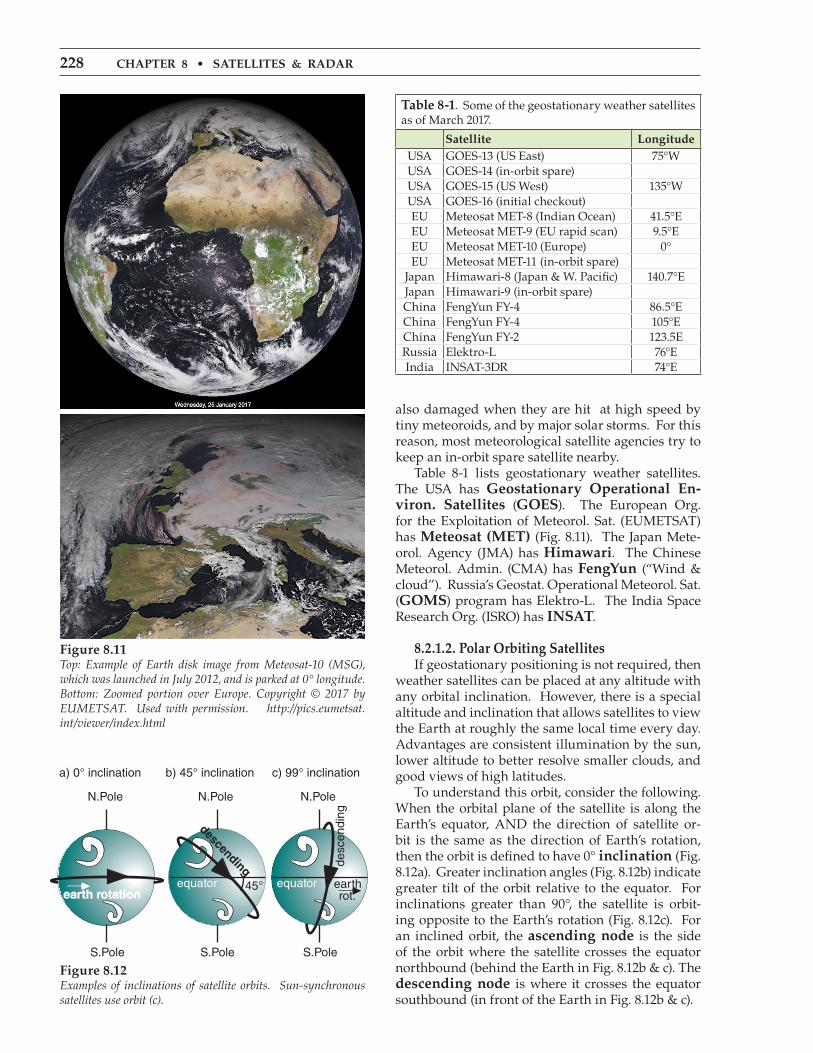
8.2.1.2.PolarOrbitingSatellites If geostationary positioning is not required, then weather satellites can be placed at any altitude with any orbital inclination. However, there is a special altitude and inclination that allows satellites to view the Earth at roughly the same local time every day. Advantages are consistent illumination by the sun, lower altitude to better resolve smaller clouds, and good views of high latitudes. To understand this orbit, consider the following. When the orbital plane of the satellite is along the Earth’s equator, AND the direction of satellite or-bit is the same as the direction of Earth’s rotation, then the orbit is defined to have 0° inclination (Fig. 8.12a). Greater inclination angles (Fig. 8.12b) indicate greater tilt of the orbit relative to the equator. For inclinations greater than 90°, the satellite is orbit-ing opposite to the Earth’s rotation (Fig. 8.12c). For an inclined orbit, the ascending node is the side of the orbit where the satellite crosses the equator northbound (behind the Earth in Fig. 8.12b & c). The descending node is where it crosses the equator southbound (in front of the Earth in Fig. 8.12b & c).
Figure 8.12Examples of inclinations of satellite orbits. Sun-synchronous satellites use orbit (c).
N.Pole
equator
N.Pole
45°
descendingequator earth
rot.
N.Pole
a) 0° inclination b) 45° inclination c) 99° inclination
desc
endi
ng
earth rotation
S.Pole S.Pole S.Pole
Figure 8.11Top: Example of Earth disk image from Meteosat-10 (MSG), which was launched in July 2012, and is parked at 0° longitude. Bottom: Zoomed portion over Europe. Copyright © 2017 by EUMETSAT. Used with permission. http://pics.eumetsat.int/viewer/index.html
Table 8-1. Some of the geostationary weather satellites as of March 2017.
Satellite LongitudeUSA GOES-13 (US East) 75°WUSA GOES-14 (in-orbit spare)USA GOES-15 (US West) 135°WUSA GOES-16 (initial checkout)EU Meteosat MET-8 (Indian Ocean) 41.5°EEU Meteosat MET-9 (EU rapid scan) 9.5°EEU Meteosat MET-10 (Europe) 0°EU Meteosat MET-11 (in-orbit spare)
Japan Himawari-8 (Japan & W. Pacific) 140.7°EJapan Himawari-9 (in-orbit spare)China FengYun FY-4 86.5°EChina FengYun FY-4 105°EChina FengYun FY-2 123.5ERussia Elektro-L 76°EIndia INSAT-3DR 74°E

R.STULL•PRACTICALMETEOROLOGY 229
Polar orbiting weather satellites are designed so that the locations of the ascending and descending nodes are sun-synchronous. Namely, the satellite always observes the same local solar times on every orbit. For example, Fig. 8.13a shows a satellite orbit with descending node at about 10:20 AM local time. Namely, the local time at city A directly under the satellite when it crosses the equator is 10:20 AM. For this sun-synchronous example, 100 minutes later, the satellite has made a full orbit and is again over the equator. However, the Earth has rotated 25.3° during this time, so it is now local noon at city A. However, city B is now under the satellite (Fig. 8.13b), where its local time is 10:20 AM. 100 minutes later, during the next orbit, city C is under the satel-lite, again at 10:20 AM local time (Fig. 8.13c). For the satellite orbits in Fig. 8.13, on the back side of the Earth, the satellite always crosses the equator at 10:20 PM local time during its ascension node. Sun-synchronous polar-orbiting satellites are nicknamed by the time of day when they cross the equator during daylight. It does not matter whether this daylight crossing is during the ascent or descent part of the orbit. For the example of Fig. 8.13, this is the morning or AMsatellite. The USA has PolarOrbitingEnviron.Satel-lite (POES) NOAA-19, launched in Feb 2009. The Suomi National Polar-orbiting Partnership (NPP) satellite (launched Oct 2011) is a transition to future Joint Polar Sat. System (JPSS) satellites. EUMETSAT has 2 Metop satellites in orbit. For the polar orbit to remain sun-synchronous during the whole year, the satellite orbit must pre-cess 360°/year as the Earth orbits the sun; namely, 0.9863° every day. This is illustrated in Fig. 8.14. Aerospace engineers, astronomers and physicists devised an ingenious way to do this without using their limited supply of on-board propellant. They take advantage of the pull of the solar gravity and the resulting slight tidal bulge of the “solid” Earth toward the sun. As the Earth rotates, this bulge (which has a time lag before disappearing) moves eastward and exerts a small gravitational pull on the satellite in the direction of the Earth’s rotation. This applies a torque to the orbit to cause it to gradually rotate relative to the fixed stars, so the orbit remains synchronous relative to the sun. The combination of low Earth orbit altitude AND incli-nation greater than 90° gives just the right amount of precession to maintain the sun-synchronous orbit. The result is that polar-orbiting weather satel-lites are usually placed in low Earth orbit at 700 to 850 km altitude, with short orbital periods of 98 to 102 minutes, and inclinations of 98.5° to 99.0°. Polar orbiting satellites do not go directly over the poles, but intentionally miss them by 9°. This is still close enough to get good images of the poles.
Figure 8.13Rotation of the Earth under a sun-synchronous satellite orbit. X marks local noon.
equator
N.Pole
c) 3rd orbit,200 min. later
N.Pole
b) 2nd orbit,100 min. later
N.Pole
a) first orbit
ABC ABCABC
localnoon
X X X
S.Pole S.Pole S.Pole
Figure 8.14Precession of polar satellite orbit (thick lines) as the Earth orbits around the sun (not to scale). The page number at the top of this textbook page can represent a “fixed star”.
N.Pole
N.Pole
N.
Pole
N.
Pole
sun
earth orbit

230 CHAPTER8•SATELLITES&RADAR
8.2.2. Imager Modern weather satellites have many capabili-ties, one of which is to digitally photograph (make images of) the clouds, atmosphere, and Earth’s surface. Meteorologists use these photos to help identify and locate weather patterns such as fronts, thunderstorms and hurricanes. Pattern-recognition programs can also use sequences of photos to track cloud motions, thereby inferring the winds at cloud-top level. The satellite instrument system that ac-quires the digital data to construct these photos is called an imager. USA geostationary GOES-16 weather satellite has 16 imager channels (wavelength bands) for view-ing the Earth system (Fig. 8.4). Some of the spec-tral bands were chosen specifically to look through different transmittance windows to “see” different atmospheric and cloud features. These channels are summarized in Table 8-2. Three bands traditionally used by forecasters are visible, IR, and water vapor. Imager channels for the European Meteosat-10 are listed in Table 8-3. This satellite has 12 channels. Included are more visible channels to better discern colors.
8.2.2.1. Visible Visible satellite images (GOES-16 channels 1 and 2) show what you could see with your eyes if you were up in space. All cloud tops look white during daytime, because of the reflected sunlight. In cloud-free regions the Earth’s surface is visible. At night, special low-light visible-channel imagers on some satellites can see city lights and moonlit clouds. Without this feature, visible images are useless at night.
8.2.2.2. Infrared (IR) Infrared satellite images (GOES channel 13) use long wavelengths in a transmittance window, and can clearly see through the atmosphere to the sur-face or the highest cloud top. There is very little so-lar energy at this wavelength to be reflected from the Earth system to the satellite; hence, the satellite sees mostly emissions from the Earth or clouds. The advantage of this channel is it is useful both day and night, because the Earth never cools to absolute zero at night, and thus emits IR radiation day and night. Images made in this channel are normally grey- shaded such that colder temperatures look whiter, and warmer looks darker. Recall that standard-at-mosphere temperature decreases as height increases in the troposphere (Chapter 1). Thus, white-colored clouds in this image indicate high clouds (cirrus, thunderstorm anvils, etc.), and darker grey clouds are low clouds (stratus, fog tops, etc.) Medium grey shading implies middle clouds (altostratus, etc.).
Table 8-2. Advanced Baseline Imager (ABI) channels/bands on USA GOES-16 weather satellite. WV = water vapor. IR = infrared. •PopularoldGOES-15channelsforvisible,WV&IR.
Chan-nel#
Nickname of the Spectral Band
Center Wave-length (µm)
Wave-length Range (µm)
1 visible blue 0.47 0.45 - 0.49
2• visible red 0.64 0.59 - 0.69
3 “veggie” 0.865 0.846 - 0.885
4 cirrus 1.378 1.371 - 1.386
5 snow/ice 1.61 1.58 - 1.64
6 cloud-particle size 2.25 2.225 - 2.275
7 shortwave IR window 3.90 3.80 - 4.00
8• high troposphere WV 6.19 5.77 - 6.6
9 mid-troposphere WV 6.95 6.75 - 7.15
10 low-troposphere WV 7.34 7.24 - 7.44
11 cloud-top phase 8.5 8.3 - 8.7
12 ozone 9.61 9.42 - 9.8
13• surface & cloud IR 10.35 10.1 - 10.6
14 longwave IR window 11.2 10.8 - 11.6
15 dirty-window IR 12.3 11.8 - 12.8
16 carbon dioxide 13.3 13.0 - 13.6
Table 8-3. Imager channels on European MSG-3 (Meteosat-10) weather satellite. VIS = visible. NIR = near infrared. IR = infrared. WV = water vapor.
Channel#
Name Center Wave-length (µm)
Wave-length Range (µm)
1 VIS 0.6 (visible orange)
0.635 0.56 - 0.71
2 VIS 0.8 (deep red) 0.81 0.74 - 0.88
3 NIR 1.6 (near IR) 1.64 1.50 - 1.78
4 IR 3.9 3.90 3.48 - 4.36
5 WV 6.2 (water va-por: high trop.)
6.25 5.35 - 7.15
6 WV 7.3 (water va-por: mid-trop.)
7.35 6.85 - 7.85
7 IR 8.7 8.70 8.30 - 9.10
8 IR 9.7 (ozone) 9.66 9.38 - 9.94
9 IR 10.8 10.80 9.80 - 11.8
10 IR 12.0 12.00 11.0 - 13.0
11 IR 13.4 (high-troposphere)
13.40 12.4 - 14.4
12 HRV (high-resolution visible)
broad-band
0.4 - 1.1
R.STULL•PRACTICALMETEOROLOGY 231
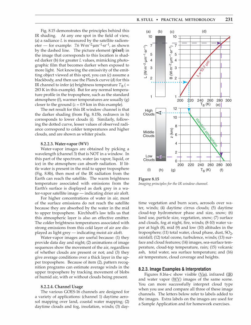
Fig. 8.15 demonstrates the principles behind this IR shading. At any one spot in the field of view, (a) a radiance L is measured by the satellite radiom-eter — for example: 7.6 W·m–2·µm–1·sr–1, as shown by the dashed line. The picture element (pixel) in the image that corresponds to this location is shad-ed darker (b) for greater L values, mimicking photo-graphic film that becomes darker when exposed to more light. Not knowing the emissivity of the emit-ting object viewed at this spot, you can (c) assume a blackbody, and then use the Planck curve (d) for this IR channel to infer (e) brightness temperature TB ( = 283 K in this example). But for any normal tempera-ture profile in the troposphere, such as the standard atmosphere (f), warmer temperatures are usually (g) closer to the ground (z = 0.9 km in this example). The net result for this IR window channel is that the darker shading (from Fig. 8.15b, redrawn in h) corresponds to lower clouds (i). Similarly, follow-ing the dotted curve, lesser values of observed radi-ance correspond to colder temperatures and higher clouds, and are shown as whiter pixels.
8.2.2.3. Water-vapor (WV) Water-vapor images are obtained by picking a wavelength (channel 3) that is NOT in a window. In this part of the spectrum, water (as vapor, liquid, or ice) in the atmosphere can absorb radiation. If lit-tle water is present in the mid to upper troposphere (Fig. 8.8b), then most of the IR radiation from the Earth can reach the satellite. The warm brightness temperature associated with emissions from the Earth’s surface is displayed as dark grey in a wa-ter-vapor satellite image — indicating drier air aloft. For higher concentrations of water in air, most of the surface emissions do not reach the satellite because they are absorbed by the water in the mid to upper troposphere. Kirchhoff’s law tells us that this atmospheric layer is also an effective emitter. The colder brightness temperatures associated with strong emissions from this cold layer of air are dis-played as light grey — indicating moist air aloft. Water-vapor images are useful because: (1) they provide data day and night; (2) animations of image sequences show the movement of the air, regardless of whether clouds are present or not; and (3) they give average conditions over a thick layer in the up-per troposphere. Because of item (2), pattern recog-nition programs can estimate average winds in the upper troposphere by tracking movement of blobs of humid air, with or without clouds being present.
8.2.2.4. Channel Usage The various GOES-16 channels are designed for a variety of applications: (channel 1) daytime aero-sol mapping over land, coastal water mapping; (2) daytime clouds and fog, insolation, winds; (3) day-
time vegetation and burn scars, aerosols over wa-ter, winds; (4) daytime cirrus clouds; (5) daytime cloud-top hydrometeor phase and size, snow; (6) land use, particle size, vegetation, snow; (7) surface and clouds, fog at night, fire, winds; (8-10) water va-por at high (8), mid (9) and low (10) altitudes in the troposphere; (11) total water, cloud phase, dust, SO2, rainfall; (12) total ozone, turbulence, winds; (13) sur-face and cloud features; (14) images, sea-surface tem-perature, cloud-top temperature, rain; (15) volcanic ash, total water, sea surface temperature; and (16) air temperature, cloud coverage and heights.
8.2.3. Image Examples & Interpretation Figures 8.16a-c show visible (Vis), infrared (IR) and water vapor (WV) images of the same scene. You can more successfully interpret cloud type when you use and compare all three of these image channels. The letters below refer to labels added to the images. Extra labels on the images are used for a Sample Application and for homework exercises.
Figure 8.15Imaging principles for the IR window channel.
200 220 240 260 280 3001
2
3
4
5
7
10
LowClouds
HighClouds
MiddleClouds
Imag
e S
hadi
ng
1
2
3
4
5
7
10
200 220 240 260 280 3000
2
4
6
8
10
12
z (k
m)
TB (K)
TB (K)
(a) (b) (c) (d)
(e)
(f)(g)(h)(i)
λ =
10.7
µm
standard atmosphere
B (
W·m
–2·µ
m–1
·sr–
1 )
L (W
·m–2
·µm
–1·s
r–1 )

232 CHAPTER8•SATELLITES&RADAR
Figure 8.16aVisible satelliteimage.
To aid image interpretation, letter labels a-z are added to identical locations in all 3 satellite images.
Figure 8.16bInfrared (IR)satelliteimage.
a
bb
b
b
c
d
e
f
g1
g2
g3
h
i
m
n
r
s
t
u
vw
x
y
z
a
bb
b
b
c
d
e
f
g1
g2
g3
h
i
m
n
r
s
t
u
vw
x
y
z
[Images a-c courtesy of Space Science & Engineering Center, Univ. of Wiscon-sin-Madison. Valid time for images: 00 UTC on 16 June 2004.]

R.STULL•PRACTICALMETEOROLOGY 233
Figure 8.16cWater-vaporsatellite image.
a
bb
b
b
c
d
e
f
g1
g2
g3
h
i
m
n
r
s
t
u
vw
x
y
z
ITCZ
Pola
r Jet
Subtropical J
et
LH
H
L
L
100°W120°Wequator
20°N
40°N
60°N
140°W
160°W
180°W
Figure 8.16dInterpretation of the satellite images. (On same scale as the images; can be copied on trans-parency and overlaid.) Symbols and acronyms will be explained in later chapters.

234 CHAPTER8•SATELLITES&RADAR
h. Tropopause Fold or Dry Air Aloft:Vis: Anything. IR: Anything.WV: Dark grey or black, because very dry air in the upper troposphere. Occurs during tropopause folds, because dry stratospheric air is mixed down.
i. High Humidities Aloft:Vis: Anything.IR: Anything.WV: Light grey. Often see meandering streams of light grey, which can indicate a jet stream. (Might be hard to see in this copy of a satellite image.)
“Image Interpretation” means the use of sat-ellite images to determine weather features such as fronts, cyclones, thunderstorms and the global cir-culation. This is a very important part of manual weather forecasting. Whole books are devoted to the subject, and weather forecasters receive exten-sive training in it. In this book, overviews of image interpretation of cyclones, fronts, and thunderstorms are covered later, in the chapters on those topics.
a. Fog or low stratus: Vis: White, because it is a cloud.IR: Medium to dark grey, because low, warm tops.WV: Invisible, because not in upper troposphere. In-stead, WV shows amount of moisture aloft.
b. Thunderstorms: Vis: White, because it is a cloud.IR: Bright white, because high, cold anvil top.WV: Bright white, because copious amounts of water vapor, rain, and ice crystals fill the mid and upper troposphere. Often the IR and WV images are en-hanced by adding color to the coldest temperatures and most-humid air, respectively, to help identify the strongest storms.
c. Cirrus, cirrostratus, or cirrocumulus: Vis: White, because cloud, although can be light grey if cloud is thin enough to see ground through it.IR: White, because high, cold cloud.WV: Medium to light grey, because not a thick layer of moisture that is emitting radiation.
d.Mid-levelcloudtops: Could be either a layer of altostratus/altocumulus, or the tops of cumulus mediocris clouds.Vis: White, because it is a cloud.IR: Light grey, because mid-altitude, medium-temperature.WV: Medium grey. Some moisture in cloud, but not a thick enough layer in mid to upper troposphere to be brighter white.
e. Space:Vis: Black (unless looking toward sun).IR: White, because space is cold.WV: White, because negligible emissions from space.
f.Snow-cappedMountains(notclouds):Vis: White, because snow is white.IR: Light grey, because snow is cold, but not as cold as high clouds or outer space.WV: Maybe light grey, but almost invisible, because mountains are below the mid to upper troposphere. Instead, WV channel shows moisture aloft.
g. Land or Water Surfaces (not clouds):g1 is in very hot desert southwest in summer, g2 is in arid plateau, and g3 is Pacific Ocean.Vis: Medium to dark grey. Color or grey shade is that of the surface as viewed by eye.IR: g1 is black, because very hot ground. g2 is dark grey, because very warm. g3 is light grey, because cool ocean.WV: Light grey or invisible, because below mid to upper troposphere. Instead, sees moisture aloft.
Sample Application Determine cloud type at locations “m” and “n” in satellite images 8.16a-c.
Find the AnswerGiven: visible, IR, and water vapor imagesFind: cloud type
m: vis: White, therefore cloud, fog, or snow. IR: White, thus high cloud top (cirrus or thunderstorm, but not fog or snow). wv: White, thus copious moisture within thick cloud layer. Thus, not cirrus. Conclusion: thunderstorm.
n: vis: White or light grey, thus cloud, fog, or snow. (Snow cover is unlikely on unfrozen Pacific). IR: Medium grey, roughly same color as ocean. Therefore warm, low cloud top. wv: Medium grey (slightly darker than surround- ing regions), therefore slightly drier air aloft. But gives no clues regarding low clouds. Conclusion: low clouds or fog.
Check: Difficult to check or confirm now. After you learn synoptics you can check if the cloud feature makes sense for the weather pattern that it is in.Exposition: This is like detective work or like a med-ical diagnosis. Look at all the clues, and rule out the clouds that are not possible. Be careful and systematic. Use other info such as the shape of the cloud or its po-sition relative to other clouds or relative to mountains or oceans. Interpreting satellite photos is somewhat of an art, so your skill will improve with practice.

R.STULL•PRACTICALMETEOROLOGY 235
However, for future reference, Fig. 8.16d shows my interpretation of the previous satellite photos. This particular interpretation shows only some of the larger-scale features. See the Fronts, Cyclones, and General Circ. chapters for symbol definitions.
8.2.4. Sounder GOES-15 has a sounder radiometer with 19 chan-nels. GOES-16 doesn’t need a separate sounder be-cause the Advanced Baseline Imager (ABI) has suf-ficient image channels to allow sounding retrievals. The different wavelength channels (Table 8-2) have different weighting functions (Fig. 8.9) that peak at different altitudes, allowing us to retrieve a sound-ing (temperatures at different altitudes). We will ex-amine the basics of this complex retrieval process. There is a limit to our ability to retrieve sounding data, as summarized in two corollaries. Corollary 1 is given at right. To demonstrate it, we will start with a simple weighting function and then gradual-ly add more realism in the subsequent illustrations. Consider the previous idealized transmittance profile (Fig. 8.7), but now divide the portion between z = 5 and 10 km into 5 equal layers. As shown in Fig. 8.17a, the change in transmittance across each small layer is ∆ τ̂ = 0.2 (dimensionless); hence, the weight (Fig. 8.17b) for each layer is also W = 0.2 . Assume that this is a crude approximation to sounder chan-nel 3, with a central wavelength of λ = 14.0 µm. Suppose the “actual” temperature of each layer, from the top down, is T = –20, –6, –14, –10, and 0°C, as illustrated by the data points and thin line in Fig. 8.17c. (Ignore the portions of the sounding below 5 km and above 10 km, because this weighting func-tion cannot “see” anything at those altitudes. Using Planck’s Law (eq. 8.1), find the blackbody radiance from each layer from the top down: B = 3.88, 4.82, 4.27, 4.54, and 5.25 W·m–2·µm–1·sr–1. Weight each by W = 0.2 and then sum according to the radi-ative transfer eq. (8.5) to compute the weighted aver-age. This gives the radiance observed at the satellite: L = 4.55 W·m–2·µm–1·sr–1. The surface (skin) term in eq. (8.5) was neglected because the transmittance from the surface is zero, so no surface information reaches the satellite for this idealized situation. This satellite-observed radiance is communicated to ground stations, where automatic computer pro-grams retrieve the temperature using eq. (8.2). When we do that, we find TB = 263.18 K , or T = –9.82°C. This is plotted as the thick line in Fig. 8.17c. Detailed temperature-sounding structure is not retrieved by satellite, because the retrieval can give only one piece of temperature data per weighting function. Vertically broad weighting functions tend to cause significant smoothing of the retrieved tem-perature sounding.
Retrieval Corollary 1: The sounder can retrieve (at most) one piece of temperature data per channel. The temperature it gives for that channel is the average brightness temperature weighted over the depth of the weighting function.
Figure 8.17Retrieval of temperature from one channel (idealized). (a) trans-mittance; (b) weighting function; (c) original (thin line with data points) and satellite retrieved (thick line) temperatures.
0
5
10
15
20
0
5
10
15
20
0
5
10
15
20
z(km)
τ W T (°C)0 1 0 0.2 –20 0
(a) (b) (c)
ˆ
INFO • Some Other Satellite Systems
Scatterometer sensors on satellites can detect capillary waves on the ocean, allowing near-surface wind speeds to be estimated. Passive and active Spe-cial Sensor Microwave Imagers (SSM/I) can retrieve precipitation and precipitable water over the ocean. Combining a series of observations while a satellite moves allows small on-board antennas to act larger, such as via synthetic aperture radar (SAR). GOES-16 has a Geostationary Lightning Mapper (GLM) that has an optical transient detector to ob-serve lightning flashes. When a lightning discharge happens, it excites oxygen atoms in the air, which then emit near IR radiation at 0.7774 µm wavelength. The GLM detector is tuned to this wavelength. This emis-sion can be observed both day and night.

236 CHAPTER8•SATELLITES&RADAR
8.2.4.1. Illustration of Retrieval Corollary 1 (Non-overlapping Weighting Functions) Consider a slightly more realistic illustration of a perfect (idealized) case where the weighting functions do not overlap vertically between differ-ent channels (Fig. 8.18a). The relationship between actual temperatures (thin line) and the resulting temperature retrievals are sketched. Namely, the weighting functions are independent of each other, allowing the four channels to retrieve four indepen-dent temperatures, as plotted by the thick line (Fig. 8.18b). The thick line is the retrieved sounding. Instead of plotting the retrieved sounding as a sequence of vertical line segments as shown in Fig. 8.19a, it is often plotted as data points. For our four independent channels, we would get four data points (large, open circles), and the resulting sounding line is drawn by connecting the circles (Fig. 8.19b). The retrieved sounding (thick line in Fig. 8.19b) does a good job of capturing the gross-features of the tem-perature profile, but misses the fine details such as sharp temperature inversions.
8.2.4.2. Illustration of Retrieval Corollary 2 (OverlappingWeightingFunctions) With non-overlapping weighting functions, the sounding-retrieval process was easy. For more re-alistic overlapping weighting functions, it becomes very difficult, as summarized in Retrieval Corol-lary 2, given in the left column. We can first study this as a forward problem, where we pretend we already know the temperature profile and want to find the radiances that the satel-lite would see. This approach is called an Observ-ing System Simulation Experiment (OSSE), used by instrument designers to help anticipate the radiances arriving at the satellite, so that they can fix problems before the satellite is launched. We antici-pate that the radiance received in one channel de-pends on the temperatures at many heights. Easy! Later, we will approach this more realistically; i.e., as an inverse problem where we have satel-lite-measured radiances and want to determine atmospheric temperatures. The inverse problem for overlapping weighting functions requires us to solve a set of coupled nonlinear equations. Nasty! To illustrate the forward problem, suppose that idealized weighting functions of Fig. 8.20 and Ta-ble 8-4 approximate GOES-15 weighting functions for sounder channels 1 – 4. For any one channel, the sum of the weights equals one, as you can check from the data in the figure. Each weighting function peaks at a different height. For simplicity, look at only the atmospheric contribution to the radiances and ignore the surface (skin) term.
Retrieval Corollary 2: If weighting functions from different channels have significant overlap in alti-tude and have similar shapes, then they do not provide independent observations of the atmosphere. For this situation, if there are also measurement errors in the ra-diances or the weighting functions, then the sounding can retrieve fewer than one piece of temperature data per sounder channel. (See the “Higher Math” box later in this section for a demonstration.)
Figure 8.18(a) Weighting functions for four idealized channels (Ch. 1 – 4). (b) Actual (thin line) and retrieved (thick line) temperature sounding.
0
5
10
15
20
Ch.4
Ch.3
Ch.2
Ch.1
T (°C)0 W 0 W 0 W 0 W
z (k
m)
(a) (b)
Figure 8.19Retrieved soundings (a, thick line), are usually plotted as (b) single data points (open circles) for each channel, connected by straight lines.
0
5
10
15
20
0
5
10
15
20
T (°C) T (°C)
(a) (b)
z(km)
z(km)

R.STULL•PRACTICALMETEOROLOGY 237
For this forward example, suppose the tempera-tures for each layer (from the top down) are T = –40, –60, –30, and +20°C, as plotted in Fig. 8.21. Namely, we are using a coarse-resolution T profile, because we already know from Corollary 1 that retrieval methods cannot resolve anything finer anyway. For each channel, we can write the radiative transfer equation (8.5). To simplify these equations, use λ = 1, 2, 3, 4 to index the wavelengths of sounder channels 1, 2, 3, 4. Also, use j = 1, 2, 3, 4 to index the four layers of our simplified atmosphere, from the top down. The radiative transfer equation for our simple 4-layer atmosphere, without the skin term, is: L B T W
jj jλ λ λ=
=∑
1
4( )· ,
(8.9)
After expanding the sum, this equation can be written for each separate channel as:
L1 = (8.10a)B1(T1)·W1,1 + B1(T2)·W1,2 + B1(T3)·W1,3 + B1(T4)·W1,4
L2 = (8.10b)B2(T1)·W2,1 + B2(T2)·W2,2 + B2(T3)·W2,3 + B2(T4)·W2,4
L3 = (8.10c)B3(T1)·W3,1 + B3(T2)·W3,2 + B3(T3)·W3,3 + B3(T4)·W3,4
L4 = (8.10d)B4(T1)·W4,1 + B4(T2)·W4,2 + B4(T3)·W4,3 + B4(T4)·W4,4
j: layer 1 layer 2 layer 3 layer 4
Because of the large vertical spread of the weights, the radiance in each channel depends on the tem-perature at many levels, NOT just the one level at the peak weight value. But the radiative transfer equa-tions are easy to solve; namely, given T and W, it is straightforward to calculate the radiances L, because we need only solve one equation at a time. I did this on a spreadsheet — the resulting radiances for each channel are in Table 8-5. Now consider the more realistic inverse prob-lem. To find the temperature T for each layer, know-ing the radiance L from each sounder channel, you must solve the whole set of coupled equations (8.10a-d). These eqs. are nonlinear with respect to tempera-ture, due to the Planck function B. The number of equations equals the number of sounder channels. The number of terms in each equation depends on how finely discretized are the sounder profiles from Fig. 8.9, which is related to the number of retrieval
Table 8-4. Idealized sounder weights W λ , j .
Vec-tor
Channel(λ)
Layer in Atmosphere (j)
1(top)
2 3 4(bottom)
A 1 0.4 0.3 0.2 0.1
B 2 0.2 0.4 0.3 0.1
C 3 0.1 0.2 0.5 0.2
D 4 0 0.1 0.3 0.6
Table 8-5. Solution of the forward radiative transfer equation for the 4-layer illustrative atmosphere. These wavelengths λ correspond to GOES-15 sounder chan-nels 1-4.
Channel λ (µm) L ( W·m–2 ·µm–1 ·sr–1 )1 14.7 2.85
2 14.4 2.87
3 14.0 3.64
4 13.7 5.40
Figure 8.20Idealized weighting functions for sounder channels (Ch) 1 – 4 .
0
5
10
15
20
0 0.5 0 0.5 0 0.5 0 0.5
)
Ch. 1 Ch. 2 Ch. 3 Ch. 4
Layer1
Layer2
Layer3
Layer4
W W W W
z(km)
Figure 8.21Hypothetical atmospherictemperature profile.
–60 20–40 –20 00
5
10
15
20
Layer 1
Layer 2
Layer 3
Layer 4
z(km)
T (°C)

238 CHAPTER8•SATELLITES&RADAR
altitudes. From Retrieval Corollary 1 there is little value in retrieving more altitudes than the number of sounder channels. For example, the GOES-16 satellite has 16 channels; hence, we need to solve a coupled set of 16 equations, each with 16 nonlinear terms. Solving this large set of coupled nonlinear equa-tions is tricky; many different methods are used by government forecast centers and satellite institutes. Here is a simple, unsophisticated, brute-force ap-proach that you can solve on a spreadsheet, which gives an approximate solution: Start with an initial guess for the temperature of each layer. The better the first guess, the quicker you will converge toward the best answer. Use those temperatures to solve the much easier forward prob-lem; namely, calculate the radiances Lλ from each eq. (8.10) separately. Calculate the squared error ( Lλ calc – Lλ obs )2 between the calculated radiances and the observed radiances from satellite for each channel, and then sum the errors to get an overall measure of the quality of the guessed temperature sounding. Next, try to reduce the overall error by modify-ing the temperature guesses. For example, vary the guessed temperature for only one atmospheric layer, until you find the temperature that gives the least total error. Then do the same for the next height, and continue doing this for all heights. Then repeat the whole process, from first height to last height, always seeking the minimum error. Keep repeating these steps (i.e., keep iterating), until the total error is either zero, or small enough (considering errors in the measured radiances).
Table 8-6. Approximate solution to the Sample Applic. inverse problem. T (°C) is air temperature. L (W·m–2·µm–1·sr–1) is radiance. Error = L(obs) – L(guess).
Height: 1 (top) 2 3 4 (bot.)T (initial guess)
–20 –20 –20 –20
T (1st iteration) –32.9 –42.9 –43.3 +2.5
T (final guess) –45 –50.1 –33.6 +20.1
Channel: 1 2 3 4L (obs) 2.85 2.87 3.64 5.40
L (from T initial guess)
3.70 3.78 3.88 3.95
error2 0.7189 0.8334 0.0591 2.114
sum of error2 3.7255
L (from T final guess)
2.84 2.93 3.60 5.39
error2 0.00009 0.00367 0.00155 0.00019
sum of error2 0.0055
Sample ApplicationGiven a 4-channel sounder with weighting functions in Fig. 8.20 & Table 8-4, having the corresponding sat-ellite-observed radiances of: L1 = 2.85, L2 = 2.87, L3 = 3.64, & L4 = 5.4 W·m–2·µm–1·sr–1. Retrieve the tempera-ture sounding.
Find the Answer:Given: L(obs) above; weights W from Table 8-4.Find: Temperatures T1 to T4 (K), where ()1 is top layer.
I did this manually by trial and error on a spread-sheet — a bit tedious, but it worked.
•First,guessastartingsoundingofT(guess) = –20°C everywhere (= 253K). See Table 8-6.•Useeqs.(8.10)tocomputeradiancesL(guess) for each channel. •ForCh.1:error2
1 = (L1 guess – L1 obs)2 ; etc. for Ch.2-4.•ComputeSum of error2 = error2
1 + error22 + etc.
This initial total error was very large ( = 3.7255 W·m–2·µm–1·sr–1). •ExperimentwithdifferentvaluesofT4 (temperature of layer 4) to find the “best” value that gives the least Sum of error2 so far. Then, keeping this “best” T4 value, experiment with T3 , finding its best value. Proceed similarly for layers 2 & 1. This completes iteration 1, as shown in Table 8-6.•KeepingthebestT1 through T3, experiment with T4 again — you will find a different “best” value. Then do layers 3, 2, & 1 in succession. This ends iteration 2.•Keepiteratingforlayers4,3,2,1.Boring.Buteachtime, the Sum of error2 becomes less and less.
As my error became small, I eventually got tired and stopped iterating. The answer is T(final guess) in Table 8-6.
Exposition: Not a perfect answer, which we know only because this exercise was contrived from an earli-er illustration where we knew the actual temperature. Why was it not perfect? It was very difficult to get the temperatures for layers 1 and 2 to converge to a sta-ble solution. Quite a wide range of temperature values for these layers gave virtually the same error, so it was difficult to find the best temperatures. This is partly related to the close similarity in weighting functions for Channels 1 and 2, and the fact that they had large spread over height with no strong peak in any one layer. The radiances from these two channels are not independent of each other, resulting in a solution that is almost singular (not well behaved in a mathematical sense; not allowing a solution). These difficulties are typical. See the “Info Box” on the next page.
Check: The actual T is given in Fig. 8.21, & listed here:
Height: 1 (top) 2 3 4 (bot.)
T (actual) –40 –60 –30 +20
T (final guess) –45 –50.1 –33.6 +20.1
R.STULL•PRACTICALMETEOROLOGY 239
Some of the difficulties in sounding retrievals are listed in the Info Box below. In spite of these dif-ficulties, satellite data make an important positive contribution to weather-forecast quality. Modern numerical weather prediction can assimilate radi-ances directly, without needed a sounding retrieval.
INFO • Satellite Retrieval Difficulties
•Radianceisanaveragefromadeeplayer,often overlapping with other layers.•Radianceobservations(indifferentchannels)are
not independent of each other.•Itisdifficulttoseparatetheeffectsoftemperature
and water-vapor variations in radiance signal.•Thereisnotauniquerelationshipbetweenthe
spectrum of outgoing radiance and atmospheric temperature and humidity profiles.
•TemperaturesarenonlinearlyburiedwithinthePlanck function (but make linear approximations).
•Radianceobservationshaveerrorscausedbyinstrument errors, sampling errors, interference by clouds, and errors in the estimation of the weight-ing functions.
•Becauseofallthesefactors,thereareaninfinitenumber of temperature profiles that all satisfy the observed radiances within their error bars. Thus, statistical estimates must be used.
•Tohelppickthebestprofile,agoodfirstguessandgood boundary conditions are critical. (Retriev-al Corollary 3: The retrieved profile looks more like the first guess than like reality.)
•Satellite-retrievedsoundingsaremostusefulinregions (such as over the oceans) lacking other in-situ observations, but in such regions it is diffi-cult to provide a good first guess. Often numerical weather forecasts are used to estimate the first guess, but such forecasts usually deviate signifi-cantly from reality over ocean data-voids.
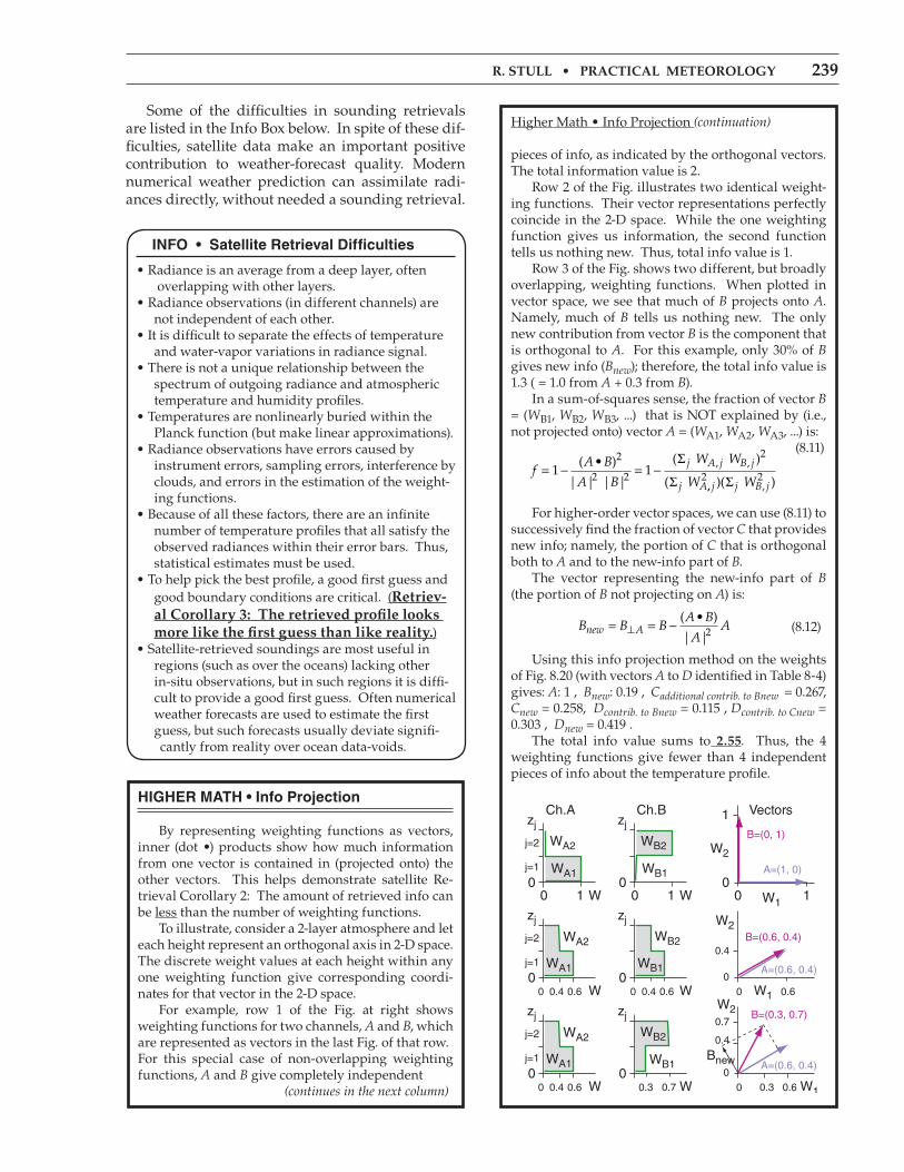
HIGHER MATH • Info Projection
By representing weighting functions as vectors, inner (dot•)products showhowmuch informationfrom one vector is contained in (projected onto) the other vectors. This helps demonstrate satellite Re-trieval Corollary 2: The amount of retrieved info can be less than the number of weighting functions. To illustrate, consider a 2-layer atmosphere and let each height represent an orthogonal axis in 2-D space. The discrete weight values at each height within any one weighting function give corresponding coordi-nates for that vector in the 2-D space. For example, row 1 of the Fig. at right shows weighting functions for two channels, A and B, which are represented as vectors in the last Fig. of that row. For this special case of non-overlapping weighting functions, A and B give completely independent (continues in the next column)
HigherMath•InfoProjection(continuation)
pieces of info, as indicated by the orthogonal vectors. The total information value is 2. Row 2 of the Fig. illustrates two identical weight-ing functions. Their vector representations perfectly coincide in the 2-D space. While the one weighting function gives us information, the second function tells us nothing new. Thus, total info value is 1. Row 3 of the Fig. shows two different, but broadly overlapping, weighting functions. When plotted in vector space, we see that much of B projects onto A. Namely, much of B tells us nothing new. The only new contribution from vector B is the component that is orthogonal to A. For this example, only 30% of B gives new info (Bnew); therefore, the total info value is 1.3 ( = 1.0 from A + 0.3 from B). In a sum-of-squares sense, the fraction of vector B = (WB1, WB2, WB3, ...) that is NOT explained by (i.e., not projected onto) vector A = (WA1, WA2, WA3, ...) is: (8.11)
f
A B
A B
W W
W
j A j B j
j A= − = −1 1
2
2 2
2( • )
| | | |
( )
( , ,Σ
Σ ,, ,)( )j j B jW2 2Σ
For higher-order vector spaces, we can use (8.11) to successively find the fraction of vector C that provides new info; namely, the portion of C that is orthogonal both to A and to the new-info part of B. The vector representing the new-info part of B (the portion of B not projecting on A) is:
B B BA B
AAnew A= = −⊥
( • )
| |2 (8.12)
Using this info projection method on the weights of Fig. 8.20 (with vectors A to D identified in Table 8-4) gives: A: 1 , Bnew: 0.19 , Cadditional contrib. to Bnew = 0.267, Cnew = 0.258, Dcontrib. to Bnew = 0.115 , Dcontrib. to Cnew = 0.303 , Dnew = 0.419 . The total info value sums to 2.55. Thus, the 4 weighting functions give fewer than 4 independent pieces of info about the temperature profile.
zj zj
W0.60.40 0.60.4
0.4
0 000
WA1
WA2
0.6W0
WB1
W1
WB2
W2
A=(0.6, 0.4)
B=(0.6, 0.4)
j=1
j=2
zj zj
W0.60.40 0.70.3
0.4
000
WA1
WA2
0.60.3
0.7
W0
WB1
W1
WB2
W2
A=(0.6, 0.4)
B=(0.3, 0.7)
j=1
j=2
zj zj
W100
Ch.A
WA1
WA2
W1 1
1
0 00 0
Ch.B Vectors
WB1
W1
WB2 W2
A=(1, 0)
B=(0, 1)
j=1
j=2
Bnew
240 CHAPTER8•SATELLITES&RADAR
8.3. WEATHER RADARS
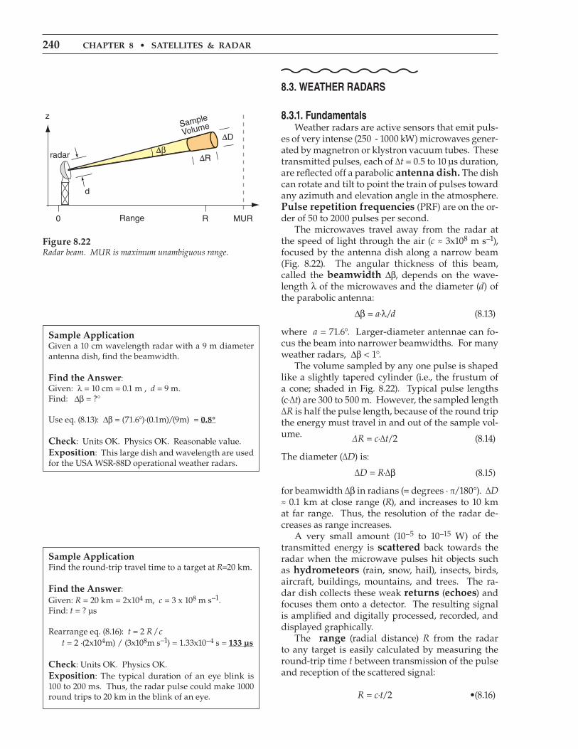
8.3.1. Fundamentals Weather radars are active sensors that emit puls-es of very intense (250 - 1000 kW) microwaves gener-ated by magnetron or klystron vacuum tubes. These transmitted pulses, each of ∆t = 0.5 to 10 µs duration, are reflected off a parabolic antenna dish. The dish can rotate and tilt to point the train of pulses toward any azimuth and elevation angle in the atmosphere. Pulse repetition frequencies (PRF) are on the or-der of 50 to 2000 pulses per second. The microwaves travel away from the radar at the speed of light through the air (c ≈ 3x10⁸ m s–1), focused by the antenna dish along a narrow beam (Fig. 8.22). The angular thickness of this beam, called the beamwidth Δβ, depends on the wave-length λ of the microwaves and the diameter (d) of the parabolic antenna:
Δβ = a·λ/d (8.13)
where a = 71.6°. Larger-diameter antennae can fo-cus the beam into narrower beamwidths. For many weather radars, Δβ < 1°. The volume sampled by any one pulse is shaped like a slightly tapered cylinder (i.e., the frustum of a cone; shaded in Fig. 8.22). Typical pulse lengths (c·∆t) are 300 to 500 m. However, the sampled length ∆R is half the pulse length, because of the round trip the energy must travel in and out of the sample vol-ume. ∆R = c·∆t/2 (8.14)
The diameter (∆D) is:
∆D = R·∆β (8.15)
for beamwidth ∆β in radians (= degrees · π/180°). ∆D ≈ 0.1 km at close range (R), and increases to 10 km at far range. Thus, the resolution of the radar de-creases as range increases. A very small amount (10–5 to 10–15 W) of the transmitted energy is scattered back towards the radar when the microwave pulses hit objects such as hydrometeors (rain, snow, hail), insects, birds, aircraft, buildings, mountains, and trees. The ra-dar dish collects these weak returns (echoes) and focuses them onto a detector. The resulting signal is amplified and digitally processed, recorded, and displayed graphically. The range (radial distance) R from the radar to any target is easily calculated by measuring the round-trip time t between transmission of the pulse and reception of the scattered signal:
R = c·t/2 •(8.16)
Sample ApplicationGiven a 10 cm wavelength radar with a 9 m diameter antenna dish, find the beamwidth.
Find the Answer:Given: λ = 10 cm = 0.1 m , d = 9 m.Find: Δβ = ?°
Use eq. (8.13): Δβ = (71.6°)·(0.1m)/(9m) = 0.8°
Check: Units OK. Physics OK. Reasonable value.Exposition: This large dish and wavelength are used for the USA WSR-88D operational weather radars.
Sample ApplicationFind the round-trip travel time to a target at R=20 km.
Find the Answer:Given: R = 20 km = 2x10⁴ m, c = 3 x 10⁸ m s–1. Find: t = ? µs
Rearrange eq. (8.16): t = 2 R / c t = 2 ·(2x104m) / (3x10⁸m s–1) = 1.33x10⁻⁴ s = 133 µs
Check: Units OK. Physics OK.Exposition: The typical duration of an eye blink is 100 to 200 ms. Thus, the radar pulse could make 1000 round trips to 20 km in the blink of an eye.
Figure 8.22Radar beam. MUR is maximum unambiguous range.
Sample
Volume
∆R
∆D
∆β
0 R MUR
z
Range
d
radar
R.STULL•PRACTICALMETEOROLOGY 241
Also, the azimuth and elevation angles to the tar-get are known from the direction the radar dish was pointing when it sent and received the signals. Thus, there is sufficient information to position each target in 3-D space within the volume scanned. Weather radar cannot “see” each individual rain or cloud drop or ice crystal. Instead, it sees the av-erage energy returned from all the hydrometeors within a finite-sized pulse subvolume. This is anal-ogous to how your eyes see a cloud; namely, you can see a white cloud even though you cannot see each individual cloud droplet. Weather radars look at three characteristics of the returned signal to help detect storms and other conditions: reflectivity, Doppler shift, and po-larization. These will be explained in detail, after first covering a few more radar fundamentals.
8.3.1.1.MaximumRange The maximum range that the radar can “see” is limited by both the attenuation (absorption of the microwave energy by intervening hydrometeors) and pulse-repetition frequency. In heavy rain, so much of the radar energy is absorbed and scattered that little can propagate all the way through (recall Beer’s Law from the Radiation chapter). The re-sulting radar shadows behind strong targets are “blind spots” that the radar can’t see. Even with little attenuation, the radar can “listen” for the return echoes from one transmitted pulse only up until the time the next pulse is transmitted. For those radars where the microwaves are gener-ated by klystron tubes (for which every pulse has exactly the same frequency, amplitude, and phase), any echoes received after this time are erroneously assumed to have come from the second pulse. Thus, any target greater than this maximum unambig-uous range (MUR, or Rmax) would be erroneously displayed a distance Rmax closer to the radar than it actually is (Fig. 8.35a). MUR is given by:
Rmax = c / [ 2 · PRF] •(8.17)
Magnetron tubes produce a more random signal that varies from pulse to pulse, which can be used to discriminate between subsequent pulses and their return signals, thereby avoiding the MUR problem.
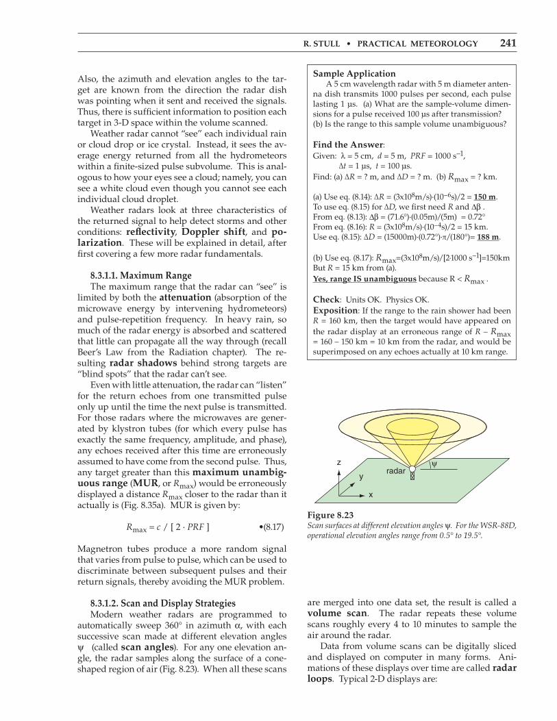
8.3.1.2. Scan and Display Strategies Modern weather radars are programmed to automatically sweep 360° in azimuth α, with each successive scan made at different elevation angles ψ (called scan angles). For any one elevation an-gle, the radar samples along the surface of a cone-shaped region of air (Fig. 8.23). When all these scans
are merged into one data set, the result is called a volume scan. The radar repeats these volume scans roughly every 4 to 10 minutes to sample the air around the radar. Data from volume scans can be digitally sliced and displayed on computer in many forms. Ani-mations of these displays over time are called radar loops. Typical 2-D displays are:
Sample Application A 5 cm wavelength radar with 5 m diameter anten-na dish transmits 1000 pulses per second, each pulse lasting 1 µs. (a) What are the sample-volume dimen-sions for a pulse received 100 µs after transmission? (b) Is the range to this sample volume unambiguous?
Find the Answer:Given: λ = 5 cm, d = 5 m, PRF = 1000 s–1, ∆t = 1 µs, t = 100 µs.Find: (a) ∆R = ? m, and ∆D = ? m. (b) Rmax = ? km.
(a) Use eq. (8.14): ∆R = (3x10⁸m/s)·(10–6s)/2 = 150 m.To use eq. (8.15) for ∆D, we first need R and Δβ . From eq. (8.13): Δβ = (71.6°)·(0.05m)/(5m) = 0.72° From eq. (8.16): R = (3x10⁸m/s)·(10–4s)/2 = 15 km. Use eq. (8.15): ∆D = (15000m)·(0.72°)·π/(180°)= 188 m.
(b) Use eq. (8.17): Rmax=(3x10⁸m/s)/[2·1000 s–1]=150kmBut R = 15 km from (a). Yes,range IS unambiguous because R < Rmax .
Check: Units OK. Physics OK.Exposition: If the range to the rain shower had been R = 160 km, then the target would have appeared on the radar display at an erroneous range of R – Rmax = 160 – 150 km = 10 km from the radar, and would be superimposed on any echoes actually at 10 km range.
Figure 8.23Scan surfaces at different elevation angles ψ. For the WSR-88D, operational elevation angles range from 0.5° to 19.5°.
ψ
x
y
zradar

242 CHAPTER8•SATELLITES&RADAR
• PPI (plan position indicator), which shows the radar echoes around 360° azimuth, but at only one elevation angle. Namely, this data is from a cone that spans many altitudes (Fig. 8.24a). These displays are often super- imposed on background maps showing towns, roads and shorelines.
• CAPPI (constant-altitude plan position indicator), which gives a horizontal slice at any altitude (Fig. 8.24b). These displays are also superimposed on background maps (Fig. 8.26). At long ranges, the CAPPI is often allowed to follow the PPI cone from the lowest elevation- angle scan.
• RHI (range-height indicator, see Fig. 8.25a), which is a vertical slice along a fixed azimuth (α) line (called a radial) from the radar. It is made by physically keeping the antenna dish pointed at one azimuth while stepping the elevation angle up and down.
•AVCS (arbitrary vertical cross section), which gives a vertical slice in any horizontal direction through the atmosphere (Fig. 8.25b).
8.3.1.3. Radar Bands In the microwave portion of the electromagnetic spectrum are wavelength (λ) bands that have been assigned for use by radar (Fig. 8.4d). Each band is given a letter designation:• L band: λ = 15 to 30 cm. Used in air traffic control and to study clear-air turbulence (CAT). •S band: λ = 7.5 to 15 cm. Detects precipitation particles, insects, and birds. Long range (roughly 500 km) capabilities, but requires a large (9 m diameter) antenna dish.•C band: λ = 3.75 to 7.5 cm. Detects precipitation particles and insects. Shorter range (roughly 250 km because the microwave pulses are more quickly attenuated by the precipitation), but requires less power and a smaller antenna dish.•X band: λ = 2.5 to 3.75 cm. Detects tiny cloud droplets, ice crystals and precipitation. Large attenuation, therefore very short range. The radar sensitivity decreases inversely with the 4th power of range.•K band is split into two parts: Ku band: λ = 1.67 to 2.5 cm Ka band: λ = 0.75 to 1.11 cm. Detects even smaller particles, but has a shorter range. (The gap at 1.11 to 1.67 cm is due to very strong absorption by a water-vapor line, causing the atmosphere to be opaque at these wavelengths; see Fig. 8.4d).
Figure 8.24(a) Plan-Position Indicator (PPI) display. (b) Constant Altitude Plan Position Indicator (CAPPI) display.
x
y
zradar
(b) CAPPI
ψ
x
y
zradar
(a) PPI
Figure 8.25(a) Range Height Indicator (RHI) display. (b) Arbitrary Verti-cal Cross Section (AVCS) display.
x
y
z radar
(a) RHI
radialα
x
y
zradar
(b) AVCS

R.STULL•PRACTICALMETEOROLOGY 243
The US National Weather Service’s nationwide network of 159 NEXRAD (Next Generation Radar) Weather Surveillance Radars (WSR-88D) uses the S band (10 cm) to detect storms and estimate pre-cipitation. The Canadian Meteorological Service is replacing their C-band (5 cm) radars with 20 S-band klystron radars. Some North American TV stations also have their own C-band weather radars. Europe is moving to a C-band standard for weather radars, although some S-band radars are also used in Spain. Weather-avoidance radars on board com-mercial aircraft are X band, to help alert the pilots to stormy weather ahead. Police radars include X and K bands, while microwave ovens use S band (12.2 cm). All bands are used for weather research.
8.3.1.4. Beam Propagation A factor leading to erroneous signals is ground clutter. These are undesired returns from fixed objects (tall towers, trees, buildings, mountains). Usually, ground clutter is found closest to the radar where the beam is still low enough to hit objects, al-though in mountainous regions ground clutter can occur at any range where the beam hits a mountain. Ground-clutter returns are often strong because these targets are large. But these targets do not move, so they can be identified as clutter and filtered out. However, swaying trees and moving traffic on a highway can confuse some ground-clutter filters. In a vacuum, the radar pulses would propagate at the speed of light in a straight line. However, in the atmosphere, the denser and colder the air, the slower the speed. A measure of this speed reduction is the index of refraction, n:
n = co / c •(8.18)
where co = 299,792,458 m s–1 is the speed of elec-tromagnetic radiation in a vacuum, and c is the speed in air. The slowdown is very small, giving index-of-refraction values on the order of 1.000325. To focus on this small change, a new variable called the refractivity, N, is defined as
N = (n – 1) x 106 •(8.19)
For example, if n = 1.000325, then N = 325. For radio waves, including microwaves:
N aPT
aeT
ae
T= − +1 2 3 2· · · •(8.20)
where P is atmospheric pressure at the beam loca-tion, T is air temperature (in Kelvin), e is water vapor pressure, a1 = 776.89 K kPa–1, a2 = 63.938 K kPa–1, and a3 = 3.75463x10⁶ K2 kPa–1. In the first term on the RHS, P/T is proportional to air density, according to
Figure 8.26CAPPI display of radar reflectivity (related to rainfall intensity) of a violent squall line of thunderstorms (orange-red curved line through center of image) sweeping across Pennsylvania in 2003. [Courtesy of the US National Weather Service.]
New YorkPennsylvania
Penn.Maryland
LakeErie
Ontario
Sample Application Find the refractivity and speed of microwaves through air of pressure 90 kPa, temperature 10°C, and relative humidity 80%.
Find the Answer:Given: P = 90 kPa, T = 10°C = 283 K, RH = 80%Find: N (dimensionless) and c (m·s–1)
First, convert RH into vapor pressure. Knowing T, get the saturation vapor pressure from Table 4-1 in the Water Vapor chapter: es = 1.233 kPa. Then use eq. (4.14): e = RH·es = 0.80·(1.233 kPa). e = 0.986 kPa Next, use P, T, and e in eq. (8.20): N= (776.89 K/kPa)·(90kPa)/(283K) – (63.938 K/kPa)·(0.986kPa)/(283K) + (3.75463x10⁶ K2/kPa)·(0.986kPa)/(283K)2 N = 247.067 – 0.223 + 46.224 = 293.068 Solve eq. (8.18) for c, and plug in n from (8.19):c = co / [1 + Nx10–6 ] = (299,792,458 m/s) / 1.000293c = 299,704,624.2 m s–1
Check: Units OK. Physics OK.Exposition: The military carefully monitors and predicts vertical profiles of refractivity to determine whether the signal from their air-defense radars would get ducted or trapped, which would prevent them from detecting enemy aircraft sneaking in above the duct.

244 CHAPTER8•SATELLITES&RADAR
the ideal gas law. The other two terms account for the polarization of microwaves by water vapor (po-larization is discussed later). The parameters in this formula have been updated to include current levels of CO2 (order of 375 ppm) in the atmosphere. Although small, the change in propagation speed through air is significant because it causes the mi-crowave beam to refract (bend) toward the denser, colder air. Recall from chapter 1 that density de-creases nearly exponentially with height, which re-sults in a vertical gradient of refractive index ∆n/∆z. This causes microwave beams to bend downward. But the Earth’s surface also curves downward rela-tive to the starting location. When estimating the beam height z above the Earth’s surface at slant range R, you must include both effects. One way to estimate this geometrically is to as-sume that the beam travels in a straight line, but that the Earth’s surface has an effective radius of curva-ture Rc of R
RR n z
k Rco
oe o=
+=
1 ·(∆ /∆ )· (8.21)
where Ro = 6371 km is the average Earth radius. The height z of the center of the radar beam can then be found from the beam propagation equation:
z z R R R R Rc c c= − + + +12 2 2 · ·sinψ (8.22)
knowing the height z1 of the radar above the Earth’s surface, and the radar elevation angle ψ. In the bottom part of the atmosphere, the verti-cal gradient of refractive index is roughly ∆n/∆z = –39x10–6 km–1 (or ∆N/∆z = –39 km–1) in a standard atmosphere. The resulting standard refraction of the radar beam gives an effective Earth radius of ap-proximately Rc ≈ (4/3)·Ro (Fig. 8.27a). Thus, ke = 4/3 in eq. (8.21) for standard conditions. Superimposed on this first-order effect are sec-ond-order effects due to temperature and humidity variations that cause changes in refractivity gradi-ent (Table 8-7). For example, when a cool humid boundary layer is capped by a hot dry temperature inversion, then conditions are right for a type of anomalous propagation called superrefraction. This is where the radar beam has a smaller radius of curvature than the Earth’s surface, and thus will bend down toward the Earth. With great enough superrefraction, the beam hits the ground and is absorbed and/or causes a
Table 8-7. Radar beam propagation conditions.
∆N/∆z (km–1) Refraction> 0 subrefraction
0 to –79 normal range–39 standard refraction
–79 to –157 superrefraction< –157 trapping or ducting
Figure 8.27(a) Standard refraction of radar beam centerline in Earth’s atmo-sphere. (b) Ducting or trapping over a smooth sea surface. (c) Trapping over a rough surface.
Earth
(b)
Earth
(c)
Earth
(a)radar beam
zR
z 1
Sample Application(§) For a radar on a 10 m tower, plot the centerline height (relative to the Earth’s surface) of the beam vs. range for standard refraction, for a 1° elevation angle.
Find the Answer:Given: ∆N/∆z = –39 km–1, z1 = 10 m = 0.01 km, Ro = 6371 kmFind: z (km) vs. R (km)
∆N/∆z = –39 km–1. Thus ∆n/∆z = –39x10–6 km–1 .Use eq. (8.21):Rc = (6371 km) / [1+(6356.766 km)(–39x10–6 km–1)] = (6371 km) · 1.33 = 8473 kmUse eq. (8.22): z = 0.01 km – 8473 km + [ R2 +(8473 km)2 + 2·R·(8473 km)·sin(1°) ]1/2
For example, z = 2.35 km at R = 100 km. Using a spreadsheet for many different R values gives:
Check: Units OK. Physics OK. Graph reasonable.Exposition: Why does the line curve up with increas-ing range? Although the radar beam bends down-ward, the Earth’s surface curves downward faster.
0 50 100 150 2000
2
4
6
z(km)
R (km)

R.STULL•PRACTICALMETEOROLOGY 245
ground-clutter return at that range if the Earth’s sur-face is rough there (Fig. 8.27c). However, for smooth regions of the Earth’s surface such as a waveless ocean, the beam can “bounce” repeatedly, which is called ducting or trapping (Fig. 8.27b). When cooler, moister air overlies warmer drier air, then subrefraction occurs, where the radius of curvature is larger than for standard refraction. This effect is limited by the fact that atmospher-ic lapse rate is rarely statically unstable over large depths of the mid and upper troposphere.
8.3.2. Reflectivity
8.3.2.1. The Radar Equation Recall that the radar transmits an intense pulse of microwave energy with power PT (≈ 750 kW for WSR-88D radars). Particles in the atmosphere scat-ter a minuscule amount of this energy back to the radar, resulting in a small received power PR. The ratio of received to transmitted power is explained by the radar equation:
· · · 2
12
1
· · ·
[ ]
=
=
−
−
−
PP
bKL
RR
ZZ
R
T a
relativereceivedpower
equipmenteffects
atmosphericeffects
rangeinversesquared
targetreflectivity
•(8.23)
where each factor in brackets is dimensionless. The most important parts of this equation are the refractive-index magnitude |K|, the range R between the radar and target, and the reflectivity factor Z. These are summarized below. The Info Box has more details on the radar equation.
|K| (dimensionless): Liquid drops are more efficient at scattering microwaves than ice crystals. |K|2 ≈ 0.93 for liquid drops, and |K|2 ≈ 0.208 for ice (assuming spherical ice particles of the same mass as the actual snow crystal).
R (km): Returned energy from more distant targets is weaker than from closer targets, as given by the inverse-square law (see Radiation chapter).
Z (mm6 m–3): Larger numbers (N) of larger- diameter (D) drops in a given volume (Vol) of air will scatter more microwave energy. This reflectivity factor is given by:
ZD
Vol
N
= ∑6
. •(8.24)
where the sum is over all N drops, and where each drop could have a different D.
INFO • Deriving the Radar Equation
The radar transmits a burst of power PT (W). As this pulse travels range R to a target drop, the energy flux (W m–2) diminishes as it spreads to cover spheri-cal surface area 4πR2, according to the inverse square law (see the Radiation chapter). But the parabolic an-tenna dish focuses the energy, resulting in antenna gain G relative to the normal spherical spread of en-ergy. While propagating to the drop, some of the en-ergy is lost along the way, as described by attenuation factor La. The net energy flux Ei (W m–2) reaching the drop is Ei = PT · G / (4πR2 · La) (R1) If that incident “power per unit area” hits a drop that has backscatter cross-sectional area σ, then power PBS (W) gets scattered in all directions: PBS = Ei · σ (R2) This minuscule burst of return power spreads to cover a spherical surface area, and is again attenuated by La while en route distance R back to the radar. The returning energy flux ER (W m–2) at the radar is ER = PBS / (4πR2 · La) (R3)Eq. (R3) is similar to (R1), except that the drop does not focus the energy, so there is no gain G. But when this flux is captured by the antenna with area Aant and focused with gain G onto a detector, the resulting received power per drop PR’ (W) is PR’ = ER · Aant · G (R4)The effective antenna area depends on many complex antenna factors, but the net result is: Aant = λ2 / [8π·ln(2)] (R5) The radar sample volume is much larger than a single drop, thus the total returned power PR is the sum over N drops: P PR R
N= ∑ ' (R6)
These N drops are contained in the sample volume Vol of air (Fig. 8.22). Assuming a cylindrical shape of length ∆R (eq. 8.14) and diameter ∆D, (eq. 8.15) gives Vol = πR2 · (∆β)2 · c · ∆t / 8 (R7)where ∆β is beam width (radians), c is microwave speed through air, and ∆t is the radar pulse duration. For hydrometeor particle diameters D less than a third of the radar wavelength λ, the backscatter cross-section area σ is well approximated by a rela-tionship known as Rayleigh scattering: σ = π5 · |K|2 · D6 / λ4 (R8)where |K| is the refractive index magnitude of the drop or ice particle.
Combining these 8 equations, and using eq. (8.24) to define the reflectivity factor Z gives the traditional form of the radar equation: (R9)
Pc P G t
RT=
∆ ∆·· ln( )
·· ·( ) ·π β
λ
3 2 2
21024 2
··
·K
L Ra
2
Z
PR = [constant] · [radar characteristics] · [atmos. char.] When the right side is multiplied by Z1/Z1 and re-arranged into dimensionless groups, the result is the version of the radar equation shown as eq. (8.23).

246 CHAPTER8•SATELLITES&RADAR
The other factors in the radar equation are as fol-lows:
Z1 = 1 mm6 m–3 is the reflectivity unit factor.
R1 = sqrt(Z1·c·∆t/λ2) (8.25) is a range factor (km), where c ≈ 3x10⁸ m s–1 is microwave speed through air. For WSR-88D radar, wavelength λ= 10 cm and pulse duration is ∆t ≈ 1.57 µs, giving R1 ≈ 2.17x10⁻¹⁰ km.
La is a dimensionless atmospheric attenuation factor (La ≥ 1) accounting for one-way losses by absorption and scattering as the microwave pulse travels between the radar and the target drop. La = 1 means no attenuation, and increasing values of La imply increasing attenuation. For example, the signal returning from a distant rain shower is diminished (appears weaker than it actually is) if it travels through a nearby shower en route to the radar. If you don’t know La, then assume La ≈ 1.
b = π3·G2·(∆β)2/[1024·ln(2)] (8.26) is a dimensionless equipment factor. For WSR-88D, the antenna gain is G ≈ 45.5 dB = 35,481 (dimensionless), and the beam width is ∆β ≈ 0.95° = 0.0161 radians, giving b ≈ 14,255.
Of most interest to meteorologists is the reflec-tivity factor Z, because a larger Z is usually associ-ated with heavier precipitation. Z varies over a wide range of magnitudes, so decibels (dB) of Z (namely, dBZ) are often used to quantify radar reflectivity:
dBZ = 10 · log(Z/Z1) •(8.27)
where this is a common logarithm (base 10). Al-though dBZ is dimensionless, the suffix “dBZ” is added after the number (e.g., 35 dBZ). dBZ can be calculated from radar measurements of PR/PT by using the log form of the radar eq.: •(8.28)
dBZPP
RR
KL
R
T a=
+
− −10 2 2
1log log log loog( )b
Although the R/R1 term compensates for most of the decrease of echo strength with distance, atmospher-ic attenuation La still increases with range. Thus dBZ still decreases slightly with increasing range. Reflectivity or echo intensity is the term used by meteorologists for dBZ, and this is what is dis-played in radar reflectivity images. Typical val-ues are –28 dBZ for haze, –12 dBZ for insects in clear air, 25 to 30 dBZ in dry snow or light rain, 40 to 50 dBZ in heavy rain, and up to 75 dBZ for giant hail.
Sample Application WSR-88D radar detects a 40 dBZ rain shower 20 km from the radar, with no other rain detected. Transmit-ted power was 750 kW, what is the received power?
Find the Answer:Given: Echo = 40 dBZ, R = 20 km, PT = 750,000 W, |K|2 = 0.93 for rain (i.e., liquid), b = 14,255 , R1 = 2.17x10⁻¹⁰ km for WSR-88D.Find: PR = ? WAssume: La = 1.0 (no attenuation), because there are no other rain showers between the radar and target.
Use eq. (8.27) and rearrange to solve for Z/Z1 : Z/Z1 = 10(dBZ/10) = 10(40/10) = 104.
Use the radar equation (8.23): PR =(7.5x10⁵W)·(14,255)·(0.93)·[(2.17x10⁻¹⁰km)/(20km)]2}·[104] PR = 1.17 x 10⁻⁸ W .
Check: Units OK. Physics OK.Exposition: With so little power coming back to the radar, very sensitive detectors are needed. WSR-88D radars can detect signals as weak as PR ≈ 10–15 W. Normal weather radars use the same parabolic an-tenna dish to receive signals as to transmit. But such an intense pulse is transmitted that the radar antenna electrically “rings” after the transmit impact for 1 µs, where this “ringing” sends strong power as a false sig-nal back toward the receiver. To compensate, the radar must filter out any received energy during the first 1 µs before it is ready to detect the weak returning echoes from true meteorological targets. For this reason, the radar cannot detect meteorological echoes within the first 300 m or so of the radar. Even when looking at the same sample volume of rain-filled air, the returned power varies considerably from pulse to pulse. To reduce this noise, the WSR-88D equipment averages about 25 sequential pulses togeth-er to calculate each smoothed reflectivity value that is shown on the radar display for each sample volume.
Sample Application For a 5 cm radar, the energy scattered from a 1 mm diameter drop is how much greater than that from a 0.5 mm drop?
Find the Answer:Given: λ = 5 cm, D1 = 0.5 mm, D2 = 1 mmFind: σscat2 / σscat1 (dimensionless)
For Rayleigh scattering [see Info Box eq. (R8)]: σscat2 / σscat1 = (D2/D1)6 = 26 = 64 .
Check: Units OK. Physics OK.Exposition: Amazingly large difference. Double the drop size and get 64 times the scattered energy.

R.STULL•PRACTICALMETEOROLOGY 247
8.3.2.2. Rainfall Rate from Radar Reflectivity A tenuous, but useful, relationship exists between rainfall rate and radar echo intensity. Both increase with the number and size of drops in the air. How-ever, this relationship is not exact. Complicating fac-tors on the rainfall rate RR include the drop termi-nal velocity, partial evaporation of the drops while falling, and downburst speed of the air containing the drops. Complicating factors for the echo intensi-ty include the bright-band effect (see next page), and unknown backscatter cross sections for complex ice-crystal shapes. Nonetheless, an empirically tuned approxima-tion can be found:
RR a a dBZ= 1 10 2· ( · ) •(8.29)
where a1 = 0.017 mm h–1 and a2 = 0.0714 dBZ–1 (both a2 and dBZ are dimensionless) are the values for the USA WSR-88D radars. This same equation can be written as: Z a RRa= 3
4· (8.30)
where a3 = 300, and a4 = 1.4, for RR in mm h–1 and Z in mm6 m–3. Equations such as (8.29) and (8.30) are called Z-R relationships. To simplify storm information presented to the public, radar reflectivities are sometimes binned into categories or levels with names or numbers representing rainfall intensities. For example, aircraft pilots and controllers use the terms in Fig. 8.28. TV weathercasters often display the intensity categories in different colors. Different agencies in different countries use different thresholds for pre-cipitation categories. For example, in Canada mod-erate precipitation is defined as 2.5 to 7.5 mm h–1. Z-R relationships can never be perfect, as is dem-onstrated here. Within an air parcel of mass 1 kg, suppose that mL = 5 g of water has condensed and falls out as rain. If that 5 g is distributed equally among N = 1000 drops, then the diameter D of each drop is 2.12 mm, from:
D
mN
L
liq=
61 3
·· ·
/
π ρ (8.31)
where ρliq = 103 kg m–3 is the density of liquid water. However, if the same mass of water is dis-tributed among N = 10,000 droplets, then D = 0.98 mm. When these two sets of N and D values are used in eq. (8.24), the first scenario gives 10 times the reflectivity Z as the second, even though they have identical total mass of liquid water mL and identical rainfall amount. Nonetheless, Z-R relationships are useful at giving a first approximation to rainfall rate.
Sample Application If radar reflectivity is 35, what is the ATC precipita-tion intensity term? Also, estimate the rainfall rate.
Find the AnswerGiven: reflectivity = 35 dBZFind: ATC term and RR = ? mm h–1.
Use Fig. 8.28: ATC weather radar term = moderateUse eq. (8.29):RR = (0.017mm h–1)·10[0.0714(1/dBZ)·35dBZ] = 5 mm h–1.
Check: Units OK. Physics OK. Exposition: Heavy and extreme echoes are often as-sociated with thunderstorms, which pilots avoid.
Sample Application Air parcels A and B both have liquid-water mixing ratio 3 g kg–1, but A has 1000 active liquid-water nuclei and B has 5,000. Compare the dBZ from both parcels.
Find the Answer:Given: rL = 3 g kg–1, ρL = 103 kg m–3 NA = 1000 , NB = 5000 .Find: dBZA and dBZB (dimensionless)Assume air density is ρ = 1 kg/m3. Assume Vol.=1 m3
Assume equal size droplets form on each nucleus, so that ΣD6 = N·D6.
Use eq. (8.31): DA=[6·(0.003kg)/(π·1000·(103 kg m–3)]1/3 = 0.00179 m = 1.79 mm (continues on next page)
Figure 8.28Precipitation-intensity terms as a function of weather-radar echo reflectivity, as used by the USA Air Traffic Control (ATC). Rainfall rate is approximate, based on eq. (8.29). For any dBZ on the horizontal axis, conceptually draw a vertical line up to the dotted line, and then look horizontally to the left to estimate the precipitation rate.
Rai
nfal
l Rat
e (m
m/h
)
0.1
1
10
100
0 10 20 30 40 50 60 70
light
moderate
heavy
extreme
ATC Weather Radar Terms
Radar Echo Intensity (dBZ)
Hail GiantHail

248 CHAPTER8•SATELLITES&RADAR
8.3.2.3. Bright Band Ice crystals scatter back to the radar only about 20% of the energy scattered by the same amount of liquid water (as previously indicated with the |K|2
factor in the radar equation). However, when ice crystals fall into a region of warmer air, they start to melt, causing the solid crystal to be coated with a thin layer of water. This increases the reflectivity of the liquid-water-coated ice crystals by a factor of 5, causing a very strong radar return known as the bright band. Also, the wet outer coating on the ice crystals cause them to stick together if they collide, resulting in a smaller number of larger-diameter snowflake clusters that contribute to even stronger returns. As the ice crystals continue to fall and completely melt into liquid drops, their diameter decreases and their fall speed increases, causing their drop density and resulting reflectivity to decrease. The net result is that the bright band is a layer of strong reflectiv-ity at the melting level of falling precipitation. The reflectivity in the bright band is often 15 to 30 times greater than the reflectivity in the ice layer above it, and 4 to 9 times greater than the rain layer below it. Thus, Z-R relationships fail in bright-band regions. In an RHI display of reflectivity (Fig. 8.29), the bright band appears as a layer of stronger returns. In a PPI display the bright band is donut shaped — a hollow circle of stronger returns around the radar, with weaker returns inside and outside the circle.
8.3.2.4. Hail Hail can have exceptionally high radar reflec-tivities, of order 60 to 75 dBZ, compared to typical maxima of 50 dBZ for heavy rain. Because hailstone size is too large for microwave Rayleigh scattering to apply, the normal Z-R relationships fail. Some radar algorithms diagnose hail for reflectivities > 40 dBZ at altitudes where the air is colder than freezing, with greater chance of hail for reflectivities ≥ 50 dBZ at altitudes where temperature ≤ –20°C.
8.3.2.5.OtherUsesforReflectivityData Radar reflectivity images are used by meteorol-ogists to identify storms (thunderstorms, hurri-canes, mid-latitude cyclones), track storm move-ment, find the height of thunderstorm features such as the top of the radar-echo (echo-top height), in-dicate likelihood of hail, and estimate rain rate and flooding potential. For example, Fig. 8.30 shows iso-lated thunderstorm cells, while Fig. 8.26 shows an organized squall line of thunderstorms. The radar image typically presented by TV weather briefers is the reflectivity image. Clear-air reflectivities from bugs can help identi-fy cold fronts, dry lines, thunderstorm outflow (gust
Missouri
Illinois
Figure 8.30CAPPI image of thunderstorm cells (orange & red), near St. Louis, MO, on 22 July 2004. White vectors indicate cell movement. (Courtesy of the US NWS.)
Sample Application (continuation)
DB=[6·(0.003kg)/(π·5000·(103 kg m–3)]1/3 = 0.00105 m = 1.05 mm
Use eq. (8.24), but using N·D6 in the numerator: ZA = 1000·(1.79 mm)6 /(1 m3) = 3.29x104 mm6 m–3 ZB = 5000·(1.05 mm)6 /(1 m3) = 6.70x103 mm6 m–3
Use eq. (8.27): dBZA = 10·log[ (3.29x104 mm6 m–3)/(1 mm6 m–3) ] = 45.2 dBZ dBZB = 10·log[ (6.70x103 mm6 m–3)/(1 mm6 m–3) ] = 38.3 dBZ
Check: Units OK. Physics OK.Exposition: Thus, the same amount of liquid water (3 g kg–1) in each parcel would lead to substantially different radar reflectivities. This is the difficulty of Z-R relationships. But not all is lost -- the polarization radar section shows how more accurate rainfall esti-mates can be made using radar.
Figure 8.29RHI sketch of the bright band in two precipitation cells. Colors mimic radar dBZ.
z
Range
bright band
0rain
ice
meltingice

R.STULL•PRACTICALMETEOROLOGY 249
fronts), sea-breeze fronts, and other boundaries (dis-cussed later in this book). Weather radar can also track bird migration. Clear-air returns are often very weak, so radar clear-air scan strategies use a slower azimuth sweep rate and longer pulse dura-tion to allow more of the microwave energy to hit the target and to be scattered back to the receiver.
8.3.3. Doppler Radar Large hydrometeors include rain drops, ice crystals, and hailstones. Hydrometeor velocity is the vector sum of their fall velocity through the air plus the air velocity itself. Doppler radars measure the component of hydrometeor velocity that is away from or toward the radar (i.e., radial velocity, Fig. 8.31). Hence, Doppler radars can detect wind com-ponents associated with gust fronts and tornadoes.
8.3.3.1. Radial Velocities Radars transmit a microwave signal of known frequency ν. But once scattered from moving hydrometeors, the microwaves that return to the ra-dar have a different frequency ν + ∆ν. Hydrometeors moving toward the radar cause higher returned frequencies while those moving away cause lower frequencies. The frequency change ∆ν is called the Doppler shift. Doppler-shift magnitude can be found from the Doppler equation: ∆ =ν
λ2· Mr •(8.32)
where λ is the wavelength (e.g., S-band radars such as WSR-88D use λ = 10 cm), and Mr is the average radial velocity of the hydrometeors relative to the ra-dar. Knowing the speed of light c = 3x10⁸ m s–1, you can find the frequency as a function of wavelength:
ν = c / λ. •(8.33)
However, the frequency shift is so minuscule that it is very difficult to measure (see Sample Application).
Sample Application An S-band radar would measure what Doppler-shift magnitude for a tornadic speed of 90 m s–1?
Find the AnswerGiven: Mr = 90 m/s, assume λ = 10 cm for S-band.Find: ∆ν = ? s–1 Use eq. (8.32): |∆ν| = [2·(90 m s–1)] / ( 0.1 m) = 1800 s–1
Check: Units & physics OK. Exposition: The Doppler-shift magnitude is less than one part per million, relative to the original transmit-ted frequency (eq. 8.33) of ν = c/λ = (3x10⁸ m s–1) / (0.1 m) = 3x10⁹ s–1.
Figure 8.31Illustration of which velocities can be seen by Doppler radar. For any location where you know the wind vector, mentally draw a circle (centered on the radar) that passes through the lo-cation, and draw a radial line (shown dashed in these figures) from the radar to the location. The radar can see only the com-ponent of the wind vector along the radial line, and cannot see the component along the circle. Examples: At point (a) the total wind vector M is along the radial line, hence the radar sees the whole wind. At point (b) the total wind vector M is tangent to the circle, hence the radar sees zero wind there. At point (c) the total wind vector M has a radial component Mr that the radar sees, and a tangential component Mtan that is invisible. Hence, only a portion of the total wind is seen there. Conversely, if you don’t know the actual wind but have Doppler radar observations, beware that an infinite number of true wind vectors can create the radial component seen by the radar. For example, at point (d) two completely different wind vectors M1 and M2 have the same radial component Mr. Hence, the radar would give you only Mr but you would have no way of knowing the total wind vector. The solution to this dilemma is to have two Doppler radars (i.e., dual Doppler) at different locations that can both scan the same wind location from different directions. The WSR-88D radar network in the USA is programmed to provide dual Doppler information.
M
radar
(tangential component; invisibleto radar)
Mr
(c)
M
M(b)
(a)
(radialcomponent
can be seen by radar)
(total wind vector)
x
y
Mtan
M1
M2 radar
Mr
M1 tan
M2 tan
(d)
x
y

250 CHAPTER8•SATELLITES&RADAR
Instead, Doppler radars detect air motion by measuring the phase shift of the microwaves. Con-sider a pulse of microwaves that scatter from a drop-let-laden air parcel (Fig. 8.32). When that parcel is at any one location and is illuminated by a radar pulse, there can be a measurable phase difference (differ-ence in locations of the wave troughs) between the incident wave and the scattered wave. Fig. 8.33a illustrates a phase difference of zero; namely, the troughs coincide. If the parcel has moved to a slightly different dis-tance from the radar when the next pulse hits, then there will be a different phase shift compared to that of the first pulse (Fig. 8.33b). As illustrated, the phase shift ∆d is twice the radial distance ∆R that the air parcel moved. You can demonstrate this to yourself by drawing a perfect wave on a thin sheet of trac-ing paper, folding the paper horizontally a certain distance ∆R from the crest, and then comparing the distance ∆d between incident and folded troughs or crests. Knowing the time between successive pulses (= 1/PRF), the radial velocity Mr is:
Mr = ∆R · PRF = PRF · ∆d/ 2 (8.34)
Table 8-8 gives the display convention for PPI or CAPPI displays of Doppler radial velocities in North America. Faster speeds are sometimes displayed with brighter lighter colors. The color convention is modeled after the astronomical “red shift” for stars moving away from Earth. In directions from the ra-dar that are perpendicular to the mean wind, there is no radial component of wind (Fig. 8.31); hence, this appears as a white or light grey line (Fig. 8.38a) of zero radial velocity (called the zero isodop). In some countries, the zero isodop is displayed with finite width as a black “no-data” line, because the ground-clutter filter eliminates the slowest radial velocities.
8.3.3.2.MaximumUnambiguousVelocity The phase-shift method imposes a maximum unambiguous velocity Mr max the radar can mea-sure, given by:
Mr max = λ·PRF/4 •(8.35)
where λ is wavelength. Fig. 8.34 shows the reason for this limitation. From the initial pulse to the sec-ond pulse, if the air parcel moved a quarter wave-length (λ/4) AWAY from the radar (Fig. 8.34b), then the scattered wave is a half wavelength out of phase from the incident wave. However, if the air parcel moved a quarter wavelength TOWARD the radar (Fig. 8.34c), then the phase shift is also half a wave-
Table 8-8. Display convention for Doppler veloci-ties.
SignofMr Radial DirectionRelative to Radar
Display Color
Positive AWAY Red & Orange
Zero (none) White, Grey or Black
Negative TOWARD Green & Blue
Figure 8.32A pulse of microwaves scatters off a stationary, droplet-laden air parcel that coincides with the radar sample volume. The same shading (solid for incident pulse, dashed for reflected pulse) is used in the next two figures.
air parcel withrain drops
Incident Pulse
Reflected Pulse
ReflectionProcess
Figure 8.33Phase shift distance is twice the distance moved by the air par-cel.
Distanceparcel moved
Phase shift distance ∆d
(a) First pulse
(b) Second pulse
∆R

R.STULL•PRACTICALMETEOROLOGY 251
length. Namely, the AWAY and TOWARD veloci-ties give exactly the same phase-shift signal at this critical speed, and the radar phase detector cannot distinguish between them. Velocities slightly faster than Mr max AWAY from the radar erroneously appear to the phase detector as fast velocities TOWARD the radar. Similarly, ve-locities faster than Mr max TOWARD the radar are erroneously folded back as fast AWAY velocities. The false, displayed velocities Mr false are: For Mr max < Mr < 2Mr max :
Mr false = Mr – 2 Mr max (8.36a)
For (– 2Mr max) < Mr < (–Mr max) :
Mr false = Mr + 2 Mr max (8.36b)
Speeds greater than 2|Mr max| fold twice. For greater max velocities Mr max , you must op-erate the Doppler radar at greater PRF (see eq. 8.35). However, to observe storms at greater range Rmax, you need lower PRF (see eq. 8.17). This trade-off is called the Doppler dilemma (Fig. 8.35). Opera-tional Doppler radars use a compromise PRF.
Sample Application A C-band radar emitting 2000 microwave pulses per second illuminates a target moving 30 m s–1 away from the radar. What is the displayed radial velocity?
Find the Answer:Given: PRF = 2000 s–1 , Mr = +30 m s–1. Assume λ = 5 cm because C-band.Find: Mr max = ? m s–1 and Mr displayed = ? m s–1
Use eq. (8.35): Mr max = (0.05 m)·(2000 s–1)/4 = 25m/s
But Mr > Mr max, therefore velocity folding.Use eq. (8.36a): Mr false = (30 m s–1) – 2·(25 m s–1) = –20 m s–1 ,where the negative sign means toward the radar.
Check: Units OK. Physics OK.Exposition: This is a very large velocity in the wrong direction. Algorithms that automatically detect tor-nado vortex signatures (TVS), look for regions of fast AWAY velocities adjacent to fast TOWARD ve-locities. However, this Doppler velocity-folding error produces false regions of adjacent fast opposite veloci-ties, causing false-alarms for tornado warnings.
Figure 8.34An air-movement distance of one quarter a wavelength toward or away from the radar can yield identical phase shifts, making velocity interpretation ambiguous (i.e., erroneous).
Phase shift
Phase shift
(a) Initialparcelposition
(b) Laterposition:parcelmovingAWAY
-or-(c) Laterposition:parcelmovingTOWARD
Figure 8.35(a) Reflectivity targets at ranges A and B from the radar appear in their proper locations. Target C, beyond the max unambigu-ous range (Rmax), is not displayed at its actual location, but ap-pears as a false echo C on the radar display closer to the radar. (b) Air parcels with negative or positive radial velocities A and B are displayed accurately. Parcel C with positive velocity greater than Mr max is falsely displayed C with large negative velocity.
0 Rmax Range
A BC C
(a) Range folding
0
A BC C
Mr+Mr max–Mr max
(b) Velocity folding

252 CHAPTER8•SATELLITES&RADAR
8.3.3.3. Velocity Azimuth Display (VAD) A plot of radial velocity Mr (at a fixed elevation angle and range) vs. azimuth angle α is called a ve-locity-azimuth display (VAD), which you can use to measure the mean horizontal wind speed and direction within that range circle. Fig. 8.36a il-lustrates a steady mean wind blowing from west to east through the Doppler radar sweep area. The re-sulting radial velocity component measured by the radar is a sine wave on the VAD (Fig. 8.36b). Mean horizontal wind speed Mavg is the ampli-tude of the sine wave relative to the average radial velocity Mr avg (=0 for this case), and the meteoro-logical wind direction is the azimuth at which the VAD curve is most negative (Fig. 8.36b). Repeating this for different heights gives the winds at differ-ent altitudes, which you can plot as a wind-profile sounding or as a hodograph (explained in the Thun-derstorm chapters). The measurements at different heights are made using different elevation angles and ranges (eq. 8.22). You can also estimate mean vertical velocity us-ing 2-D horizontal divergence determined from the VAD. Picture the scenario of Fig. 8.37a, where there is convergence (i.e., negative divergence) super-imposed on the mean wind. Namely, west winds exist everywhere, but the departing winds east of the radar are slower than the approaching winds from the west. Also, the winds have a convergent north-south component. When plotted on a VAD, the result is a sine wave that is displaced in the ver-tical (Fig. 8.37b). Averaging the slower AWAY radial winds with the faster TOWARD radial winds gives a negative average radial velocity Mr avg, as shown by the dashed line in Fig. 8.37b. Mr avg is a measure of the divergence/convergence, while Mavg still mea-sures mean wind speed. Due to mass continuity (discussed in the Atmo-spheric Forces & Winds chapter), an accumulation of air horizontally into a volume requires upward mo-tion of air out of the volume to conserve mass (i.e., mass flow in = mass flow out). Thus:
∆ =−
∆wM
Rz
r avg2·· (8.37)
where ∆w is change in vertical velocity across a lay-er of thickness ∆z, and R is range from the radar at which the radial velocity Mr is measured. Upward vertical velocities (associated with hor-izontal convergence and negative Mr avg) enhance cloud and storm development, while downward vertical velocities (subsidence, associated with hor-izontal divergence and positive Mr avg) suppress clouds and provide fair weather. Knowing that w = 0 at the ground, you can solve eq. (8.37) for w at
Sample Application From a 1 km thick layer of air near the ground, the average radial velocity is –2 m s–1 at range 100 km from the radar. What is the vertical motion at the layer top?
Find the Answer:Given: R = 100 km , ∆z = 1 km , Mr avg = –2 m s–1.Find: w = ? m s–1 at z = 1 km.Assume: wbot = 0 at the ground (at z = 0).
Use eq. (8.37): ∆w = –2·(–2 m s–1) · (1 km) / (100 km) ∆w = +0.04 m s–1. But ∆w = wtop – wbot . Thus: wtop = +0.04 m s–1
Check: Units OK. Physics OK.Exposition: This weak upward motion covers a broad 100 km radius circle, and would enhance storms.
Figure 8.36(a) Scenario of mean winds relative to radar. (b) Velocity-azi-muth display (VAD) of radial wind component. Mr is positive for wind AWAY from the radar.
0
Mr
α90° 180° 270° 360°0°
Mavgwind direction
x
y
α0°
90°
180°
270°radar
mean wind
(a) Scenario
(b) VAD
Mavg
Figure 8.37(a) Scenario of mean winds AND 2-D horizontal convergence. (b) Velocity-azimuth display (VAD) of radial wind component.
x
y
α
0°
90°
180°
270°radar
wind
(a) Scenario
(b) VAD
0
Mr
Mr avg
α180° 270° 360°0°
mean wind direction
Mavg

R.STULL•PRACTICALMETEOROLOGY 253
height ∆z above ground. Then, starting with that vertical velocity, you can repeat the calculation us-ing average radial velocities at a higher elevation an-gle to find w at this higher altitude. Repeating this gives the vertical velocity profile. A single Doppler radar cannot measure the full horizontal wind field, because it can “see” only the radial component of velocity. However, if the scan regions of two nearby Doppler radars overlap, then in theory the horizontal wind field can be calculated from this dual-Doppler information, and the full 3-D winds can be inferred using mass continuity.
8.3.3.4. Identification of Storm Characteristics While the VAD approach averages the winds within the whole scan circle, you can also use the smaller scale patterns of winds to identify storm characteristics. For example, you can use Doppler information to help detect and give advanced warn-ing for tornadoes and mesocyclones (see the Thunderstorm chapters). A single Doppler radar cannot see the whole rotation inside the thunder-storm — just the portions of the vortex with com-ponents moving toward or away from the radar. But you can use this limited information to define a tornado vortex signature (TVS, Fig. 8.38b) with the brightest red and green pixels next to each other, and with the zero isodop line passing through the tornado center and following a radial line from the radar. Hurricanes also exhibit these rotational charac-teristics, as shown in Fig. 8.39. Winds are rotating counterclockwise around the eye of this Northern Hemisphere hurricane. The zero isodop passes through the radar location in the center of this im-age, and also passes through the center of the eye of the hurricane. See the Tropical Cyclone chapter for details. Cold-air downbursts from thunderstorms hit the ground and diverge (spread out) as damag-ing horizontal straight-line winds (Fig. 8.38c). The leading edge of the outflow is the gust front. Doppler radar sees this as neighboring regions of opposite moving radial winds, similar to the TVS but with the zero isodop perpendicular to the radial from the radar, and with the green region always closer to the radar than the red region.
Figure 8.38PPI or CAPPI radar image interpretation. The white circle in-dicates the radar location. Red shaded regions indicate wind components AWAY from the radar. Green (or blue on some dis-plays) indicate a wind components TOWARD the radar. Dark-er shadings represent slower radial wind components. Actual wind directions are shown by the black arrows. (a) Uniform mean wind in the domain. (b) Tornado T vortex, surrounded by weaker mesocyclone vortex (large circle). (c) Downburst D and gust front (dashed line) at the leading edge of outflow air.
OO
greenorblue
wind zero isodop
radar red
x
y
(a) Mean Wind
x
ygreen
or blue
zero
isodop
radar
red
(b) Tornado
vortexrotationdirection
T
x
y
radar
(c) Downburst
zero
isodop
red
greenor blue
gust front
D
Sample Application A downburst and outflow are centered directly over a Doppler radar. Sketch the Doppler display.
Find the Answer:Given: Air diverging in all directions from radarSketch: Doppler radar display appearance
At every azimuth from the radar,air is moving AWAY. Thus red would be all around the radar,out to the gust front. Thefastest outflow (sketched asthe lightest red) is likely to be closest to the radar.
Check: Sketch consistent with display definitions.Exposition: Meteorologists at the radar might wor-ry about their own safety, and about radome damage. The radome is the spherical enclosure that surrounds the radar antenna, to protect the radar from the weath-er. Also, a wet radome causes extra attenuation, mak-ing it difficult to see distant precipitation echoes.
x
y
gust front
Dradar
red

254 CHAPTER8•SATELLITES&RADAR
8.3.3.5. Spectrum Width Another product from Doppler radars is the spectrum width. This is the variance of the Dop-pler velocities within the sample volume, and is a measure of the intensity of atmospheric turbulence inside storms. Also, the Doppler signal can be used with reflectivity to help eliminate ground clutter. For high elevation angles and longer pulse lengths, the spectrum width is also large in bright bands, be-cause the different fall velocities of rain and snow project onto different radial velocities. Strong wind shear within sample volumes can also increase the spectrum width.
8.3.3.6. Difficulties Besides the maximum unambiguous velocity problem, other difficulties with Doppler-estimat-ed winds are: (1) ground clutter including vehicles moving along highways or ocean waves approach-ing shore; (2) lack of information in parts of the at-mosphere where there are no scatterers (i.e., no rain drops or bugs) in the air; and (3) scatterers that move at a different speed than the air, such as falling rain-drops or migrating birds.
Sample Application Explain the “S” shape of the portion of the zero isodop line that is close to the radar in Fig. 8.39b.
Find the Answer:Given: Doppler velocities in Fig. 8.39b.Find: Explanation for “S” curve of zero isodop.
For a PPI display, the radar is observing the air along the surface of an inverted scan cone (Fig. 8.24a). Hence, targets at closer range to the radar correspond to targets at lower altitude. Curvature in the zero isodop indicates vertical shear of the horizontal winds (called wind shear for short). Close to the radar the zero isodop is aligned north-west to southeast. The wind direction at low altitude is perpendicular to this direction; namely, from the northeast at low altitude. Slightly farther from the radar (but still on the ra-dar side of the eye), the zero isodop is south-southeast to the south of the radar, and is north-northwest on the north side. The winds at this range are perpendicu-lar to a straight line drawn from the radar to the zero isodop; namely, the wind is from the east-northeast at mid altitudes.
Exposition: As you will see in the Winds & Hurri-cane chapters, boundary-layer winds feel the effect of drag against the ground, and have a direction that spirals in toward the eye. Above the boundary layer, in the middle of the troposphere, winds circle the eye.
Florida
eye
(a) Reflectivity
>40
dB
Z
KMLB
Figure 8.39Radar images of Hurricane Francis at 0300 UTC on 5 September 2004 as the eye is approaching the coast of Florida, USA. Hurri-cane intensity at this time was category 2 on the Saffir-Simpson scale, although it had been category 4 before reaching the coast. The Melbourne, FL, radar KMLB is in the center of the radar image, as indicated with the white dot. (a) PPI image of reflectivity (dBZ). (b) Doppler radial velocities. [Adapted from US National Weather Service data as displayed by the Research Applications Program division of the US National Center for Atmospheric Research.]
>25m/stoward
10m/s
eye
20m/s
Florida (b) Doppler Velocity
20m/s
>25m/saway

R.STULL•PRACTICALMETEOROLOGY 255
8.3.4. Polarimetric Radar Because Z-R relationships are inaccurate and do not give consistent results, other methods are used to improve estimates of precipitation type and rate. One method is to transmit microwave pulses with different polarizations, and then compare their re-ceived echo intensities. Radars with this capability are called polarimetric, dual-polarization, or polarization-diversity radars. Recall that electromagnetic radiation consists of perpendicular waves in the electric and magnetic fields. Polarization is defined by the direction of the electric field. Radars can be designed to switch between two or three polarizations: horizontal, vertical, and circular (see Fig. 8.40). Air-traffic control radars use circular polarization, because it partially filters out the rain, allowing a clearer view of aircraft. Most weather radars use horizontal and vertical linear polarizations. Horizontally polarized pulses get information about the horizontal dimension of the precipitation particles (because the energy scattered depends mostly on the particle horizontal size). Similarly, vertically polarized pulses get information about the vertical dimension. By alternating between hori-zontal and vertical polarization with each successive transmitted pulse, algorithms in the receiver can use echo differences to estimate the average shape of precipitation particles in the sample volume. Only the smallest cloud droplets are spherical (Fig. 8.41a, equal width and height). These would give returns of equal magnitude for both horizon-tal and vertical polarizations. However, larger rain drops become more oblate (Fig. 8.41b, flattened on the bottom and top) due to air drag when they fall. The largest drops are shaped like a hamburger bun (Fig. 8.41c). This gives greater reflectivity factor ZH from the horizontally polarized pulses than from the vertically polarized ones ZV. The amount of oblateness increases with the mass of water in the drop. There is some evidence that just before the largest drops break up due to air drag, they have a parachute or jelly-fish-like shape (Fig. 8.41d). Some hydrometeor shapes change the polariza-tion of the scattered pulse. For example, clockwise circular polarized transmitted pulses are scattered with counterclockwise circular polarization by any rain drops that are nearly spherical. Tumbling, par-tially melted, irregularly shaped ice crystals can re-spond to horizontally polarized pulses by returning a portion of the energy in vertical polarization. Dif-ferent shapes of ice crystals have different reflectiv-ity factors in the vertical and horizontal. Four variables are often analyzed and dis-played on special radar images to help diagnose hydrometeor structure and size. These are:
Figure 8.40Polarization of microwaves, where E = electric field, M = mag-netic field, and c = wave propagation at speed of light. (a) Vertical; (b) Horizontal; and (c) Circular polarization.
(a) VerticalPolarization
E
M
c
(b) HorizontalPolarization
E
M
c
(c) Circular Polarization
c
E
E
E
EE
E
E
M M
MM
MM
M
Figure 8.41Enlargement of raindrop shapes vs. diameter D (approximate). (a) D < 1 mm; (b) 1 mm < D < 3 mm ; (c) 3 mm < D; (d) large (D ≈ 4 mm) jellyfish-like shape just before drop breaks up..
(a) (b) (c)
(d)

256 CHAPTER8•SATELLITES&RADAR
•Differential Reflectivity: ZDR (unit: dB)
ZDR = 10·log(ZHH/ZVV) •(8.38)
where the first and second subscripts of reflectivity Z on the right hand side give the polarization (H = horizontal; V = vertical) of received and transmitted pulses, respectively. Typical values: –2 to +6 dB, where negative and positive values indicate vertical or horizontal orientation of the hydrometeor’s major axis. Useful with Z for improving rain-rate estimates and identifying radar attenuation regions.
•Linear Depolarization Ratio. LDR (unit: dB)
LDR = 10·log(ZVH/ZHH) •(8.39)
Typical values: > –10 dB for ground clutter –15 dB for melting snowflakes –20 to –26 dB for melting hail < –30 dB for rain Useful for estimating micrometeor type or habit. Can also help remove ground clutter and identify the bright band.
•Specific Differential Phase: KDP (unit: degrees of phase shift per 1 km path) Relative amount of phase shift (shift of the crests of the electromagnetic waves) in the returned echoes from the horizontally vs. vertically transmitted pulses. Typical values: –1 to +6 °/km, where positive values indicate oblate (horizontally dominant) hydrometeors. Tumbling hail appears symmetric on average, resulting in KDP = 0. Improves accuracy of rain rate estimate and helps to isolate the portion of echo associated with rain in a rain/hail mixture.
•Co-polar Correlation Coefficient: ρHV (unit: dimensionless, in range –1 to +1 ) Measures the amount of similarity in variation of the time series of received signals from the horizontal vs. vertical polarizations. Typical values of |ρHV|: 0.5 means very large hail 0.7 to 0.9 means drizzle or light rain 0.90 to 0.95 means hail or bright-band mix ≥ 0.95 means rain, snow, ice pellets, graupel 0.95 to 1.0 means rain Useful for estimating radar-beam attenuation and the heterogeneity of micrometeors (mixtures of differently shaped ice crystals and rain drops) in the sampling volume.
Sample Application Polarization radar measures reflectivity factors of ZHH = 1000 dBZ , ZVV = 398 dBZ , and ZVH = 0.3 dBZ. (a) Find the differential reflectivity and the linear de-polarization ratio. (b) Discuss characteristics of the hydrometeors. (c) What values of specific differential phase and co-polar correlation coefficient would you expect? Why?
Find the Answer:Given: ZHH = 1000 dBZ, ZVV = 398 dBZ , and ZVH = 0.3 dBZFind: ZDR = ? dB, LDR = ? dB
(a) Use eq. (8.38): ZDR = 10·log(1000 dBZ/398 dBZ) = +4.0 dB
Use eq. (8.39): LDR = 10·log(0.3 dBZ/1000 dBZ) = –35.2 dB
(b) Discussion: The positive value of ZDR indicates a hydrometeor with greater horizontal than vertical di-mension, such as large, oblate rain drops. The very small value of LDR supports the inference of rain, rath-er than snow or hail.
(c) I would expect KDP = 2to4°/km, because of large oblate rain drops.
I would also expect ρHV = 0.95 , because rain intensity is light to moderate, based on eq. (8.27): dBZ = 10·log(ZHH/Z1) = 10·log(1000dBZ/1dBZ) = 30 dBZ, which is then used to find the inten-sity classification from Fig. 8.28. Check: Units OK. Results reasonable for weather.Exposition: See item (b) above. In eq. (8.27) I used ZHH because the horizontal drop dimension is the one that is best correlated with the mass of the drop, as illustrated in Fig. 8.41.
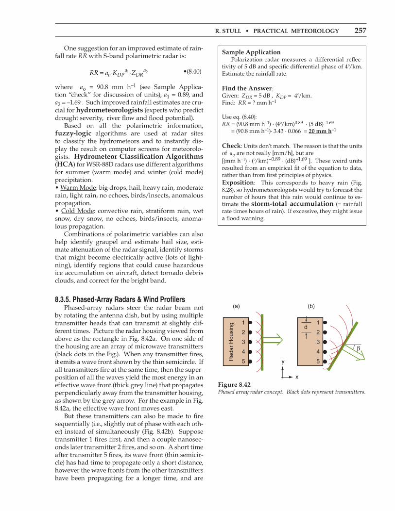
R.STULL•PRACTICALMETEOROLOGY 257
One suggestion for an improved estimate of rain-fall rate RR with S-band polarimetric radar is:
RR a K Zo DPa
DRa= · ·1 2 •(8.40)
where ao = 90.8 mm h–1 (see Sample Applica-tion “check” for discussion of units), a1 = 0.89, and a2 = –1.69 . Such improved rainfall estimates are cru-cial for hydrometeorologists (experts who predict drought severity, river flow and flood potential). Based on all the polarimetric information, fuzzy-logic algorithms are used at radar sites to classify the hydrometeors and to instantly dis-play the result on computer screens for meteorolo-gists. Hydrometeor Classification Algorithms (HCA) for WSR-88D radars use different algorithms for summer (warm mode) and winter (cold mode) precipitation. •Warm Mode: big drops, hail, heavy rain, moderate rain, light rain, no echoes, birds/insects, anomalous propagation.•Cold Mode: convective rain, stratiform rain, wet snow, dry snow, no echoes, birds/insects, anoma-lous propagation. Combinations of polarimetric variables can also help identify graupel and estimate hail size, esti-mate attenuation of the radar signal, identify storms that might become electrically active (lots of light-ning), identify regions that could cause hazardous ice accumulation on aircraft, detect tornado debris clouds, and correct for the bright band.
8.3.5. Phased-Array Radars & Wind Profilers Phased-array radars steer the radar beam not by rotating the antenna dish, but by using multiple transmitter heads that can transmit at slightly dif-ferent times. Picture the radar housing viewed from above as the rectangle in Fig. 8.42a. On one side of the housing are an array of microwave transmitters (black dots in the Fig.). When any transmitter fires, it emits a wave front shown by the thin semicircle. If all transmitters fire at the same time, then the super-position of all the waves yield the most energy in an effective wave front (thick grey line) that propagates perpendicularly away from the transmitter housing, as shown by the grey arrow. For the example in Fig. 8.42a, the effective wave front moves east. But these transmitters can also be made to fire sequentially (i.e., slightly out of phase with each oth-er) instead of simultaneously (Fig. 8.42b). Suppose transmitter 1 fires first, and then a couple nanosec-onds later transmitter 2 fires, and so on. A short time after transmitter 5 fires, its wave front (thin semicir-cle) has had time to propagate only a short distance, however the wave fronts from the other transmitters have been propagating for a longer time, and are
Sample Application Polarization radar measures a differential reflec-tivity of 5 dB and specific differential phase of 4°/km. Estimate the rainfall rate.
Find the Answer:Given: ZDR = 5 dB , KDP = 4°/km.Find: RR = ? mm h–1
Use eq. (8.40): RR = (90.8 mm h–1) · (4°/km)0.89 · (5 dB)–1.69 = (90.8 mm h–1)· 3.43 · 0.066 = 20 mm h–1
Check: Units don’t match. The reason is that the units of ao are not really [mm/h], but are [(mm h–1) · (°/km)–0.89 · (dB)+1.69 ]. These weird units resulted from an empirical fit of the equation to data, rather than from first principles of physics.Exposition: This corresponds to heavy rain (Fig. 8.28), so hydrometeorologists would try to forecast the number of hours that this rain would continue to es-timate the storm-total accumulation (= rainfall rate times hours of rain). If excessive, they might issue a flood warning.
Figure 8.42Phased array radar concept. Black dots represent transmitters.
y
x
1
2
3
4
5
1
2
3
4
5
(a) (b)
d
β
Rad
ar H
ousi
ng

258 CHAPTER8•SATELLITES&RADAR
further away from the housing. The superposition of the individual wave fronts now yields an effec-tive wave front (thick grey line) that is propagating toward the southeast. Let ∆t be the time delay between firing of subse-quent transmitters. For transmitter elements spaced a distance d from each other, the time delay need-ed to give an effective propagation angle β (see Fig. 8.42b) is: ∆t = (d/c)·sin(β) (8.41)
where c ≈ 3x10⁸ m s–1 is the approximate speed of microwaves through air. By changing ∆t, the beam (grey arrow) can be steered over a wide range of angles. Negative ∆t steers the beam toward the northeast, rather than southeast in this example. Also, by having a 2-D ar-ray of transmitting elements covering the whole side of the housing, the beam can also be steered upward by firing the bottom elements first. Two advantages of this approach are: (1) fewer moving parts, therefore less likelihood of mechan-ical failure; and (2) the beam angle can be changed instantly — allowing faster scans. However, to see a full 360° azimuth around the radar site, phased-ar-ray transmitting elements must be designed into all 4 outside walls of the radar building. While the military have used phased array radars for de-cades to detect aircraft and missiles, these radars are just beginning to be used in civilian meteorology. The US National Weather Service hopes to replace their 1988-vintage WSR-88D radars with modern multi-function phased-array weather radars.
Another phased-array application to meteorolo-gy is the wind profiler. This observes horizontal wind speed and direction at many heights by mea-suring the Doppler shifts in the returned signals from a set of radio beams tilted slightly from vertical (Fig. 8.43). Some wind profilers look like a forest of TV an-tennas sticking out of the ground, others like win-dow blinds laying horizontally, others like a large trampoline, and others like a grid of perpendicular clothes lines on poles above the ground (Fig. 8.43). Each line is a radio transmitter antenna, and the ef-fective beam can be steered away from vertical by phased (sequential) firing of these antenna wires. Wind profilers work somewhat like radars — sending out pulses of radio waves and determining the height to the clear-air targets by the time delay between transmitted and received pulses. The tar-gets are turbulent eddies of size equal to half the radio wavelength. These eddies cause refractivity fluctuations that scatter some of the radio-wave en-ergy back to receivers on the ground; hence, bugs or raindrops are not needed as targets.
Sample Application What time delay is needed in phased array radar to steer the beam 30° away from the line normal (perpen-dicular) to the radar face, if the transmitter elements are 1 m apart?
Find the Answer:Given: β = 30°, d = 1 m , c = 3x10⁸ m s–1
Find: ∆t = ? s
Use eq. (8.41): ∆t = [(1m)/(3x108 m s–1)]·sin(30°) ∆t = 1.67x10⁻⁹ s = 1.67 ns.
Check: Units OK. Physics OK. Agrees with Fig. 8.42.Exposition: The larger the angle β, the smaller the effective size of the transmitter face, and the less fo-cused is the beam. This is a disadvantage of phased-array radars used for meteorology: the sample volume changes not only with range but also with direction β. Therefore, the algorithms used to interpret meteo-rological characteristics (reflectivity, Doppler velocity, spectrum width, polarimetric data) must be modified to account for these variations.
Figure 8.43Wind profiler concept.
z
xy
North
SouthEastWest
Vertical
wind
beams
antenna wires

R.STULL•PRACTICALMETEOROLOGY 259
Wind profilers with 16 km altitude range use Very High Frequencies (VHF) of about ν = 50 MHz (λ = c/ν = 6 m). Other tropospheric wind profil-ers use an Ultra High Frequency (UHF) near 400 MHz (λ = 0.75 m = 75 cm). Smaller boundary-layer wind profilers for sampling the lower troposphere use an ultra high frequency near 1 GHz (λ = 30 cm). Normally, wind profilers are designed to trans-mit in only 3, 4 or 5 nearly-vertical, fixed beam direc-tions (Fig. 8.43). The fixed zenith angle of the slight-ly tilted beams is on the order of ζ = 14° to 24°. The radial velocities Meast and Mwest measured in the east- and west-tilted beams, respectively, are affected by the U component of horizontal wind and by vertical velocity W. Positive W (upward motion; thick grey vector in Fig. 8.44) projects into positive (away from wind profiler) components of radial ve-locity for both beams (thin grey vectors). However, positive U (thick black vector) wind contributes pos-itively to Meast, but negatively (toward the profiler) to Mwest (thin black vectors). Assume that both beams measure the same air parcel at nearly the same instant, and thus detect the same average U and W. Design the profiler so that all tilted beams have the same zenith angle. Use the measured radial velocities from a pair of oppositely tilted beams. By adding and subtracting these two measured velocities ( Meast , Mwest ), you can solve for the desired wind components (U, W):
UM Meast west=
−2·sinζ
•(8.42a)
WM Meast west=
+2·cosζ
•(8.42b)
Use similar equations with radial velocities from the north- and south-tilted beams to estimate V and W. Fig. 8.45 shows sample wind-profiler output.
Sample Application A wind profiler with 20° beam tilt uses the Doppler shift to measure radial velocities of 3.326 m s–1 and –3.514 m s–1 in the east- and west-tilted beams, respec-tively, at height 4 km above ground. Find the vertical and horizontal wind components at that height.
Find the Answer:Given: Meast= 3.326 m s–1, Mwest= –3.514 m s–1, ζ = 20°Find: U = ? m s–1 and W = ? m s–1.
Use eq. (8.42a): U = [(3.326 m s–1) – (–3.514 m s–1)]/[2·sin(20°)]=10 m s–1
Use eq. (8.42b): W=[(3.326 m s–1)+(–3.514 m s–1)]/[2·cos(20°)]=–0.1 m s–1
Check: Units OK. Physics OK.Exposition: The positive U component indicates a west wind (i.e., wind FROM the west) at z = 4 km. Neg-ative W indicates subsidence (downward moving air). These are typical of fair-weather conditions under a strong high-pressure system. Typical wind profilers make many measurements each minute, and then av-erage their results over 5 minutes to 1 hour.
Figure 8.45Wind profiler observations for Wolcott, IN. Arrow shows hori-zontal wind direction. Each short wind barb = 5 m/s, long = 10 m/s, & pennant = 50 m/s. (E.g., wind at z = 10 km, t = 02 UTC is 45 m/s from southwest.) Courtesy of US National Oceanic and Atmospheric Admin. (NOAA) Profiler Network (NPN).
12
10
8
6
4
2z
(km
)
09 08 07 06 05 04 03 02 01Time (UTC) on 31 July 2004
Figure 8.44Projections of horizontal wind U and vertical velocity W to the radial wind directions Mwest and Meast along wind-profiler west- and east-tilted beams. Mwest and Meast are positive when pointed upward.
WW
U
U
MeastMwest
ζ
ζζ
ζ
x
z

260 CHAPTER8•SATELLITES&RADAR
8.5. HOMEWORK EXERCISES
8.5.1. Broaden Knowledge & ComprehensionB1. Search the web for graphs of transmittance for wavelengths greater than 100 cm (like Figs. 8.4), and find the names of these regions of the electromag-netic spectrum. Comment on the possibility for re-mote sensing at these longer wavelengths.
B2. Search the web for graphs of weighting func-tions for one of the newer weather satellites, as spec-ified by your instructor. Discuss their advantages and disadvantages compared to the weighting func-tions given in this book.
B3. Search the web for current orbital characteristics for the active weather satellite(s) specified by your instructor. Also, look for photos or artist drawings of these satellites.
B4. Search the web for data to create tables that list the names and locations (longitude for GOES; equa-tor crossing times for POES) currently active weath-er satellites around the world. Discuss any gaps in worldwide weather-satellite coverage.
B5. Search the web for images from all the differ-ent channels for one of the satellites, as specified by your instructor. Discuss the value and utility of each image.
B6. Search the web for satellite loops that cover your location. Compare these images with the weather you see out the window, and make a short-term fore-cast based on the satellite loop.
B7. Search the web to find the most recent set of vis-ible, IR, and water-vapor images that covers your area. Print these images; label cloud areas as (a), (b), etc.; and interpret the clouds in those images. For the cloud area directly over you, compare you satel-lite interpretation with the view out your window.
B8. Search the web for thermo diagrams showing temperature soundings as retrieved from satellite sounder radiance data. Compare one of these sound-ings with the nearest rawinsonde (in-situ) sounding (by searching on “upper air” soundings).
B9. Search the web for tutorials on satellite-image interpretation; learn how to better interpret one type of cloud system (e.g., lows, fronts, thunderstorms); and write a summary tutorial for your classmates.
8.4. REVIEW
Passive sensors on weather satellites observe many different wavelengths of electromagnetic radi-ation upwelling from the Earth-ocean-atmosphere-cloud system. Imager sensors take high-quality dig-ital photographs of clouds and air motion, for which the most important wavelength channels are visible, IR, and water-vapor. Sounder radiometers remotely probe different depths in the atmosphere. For reflected visible sunlight and for wave-lengths in IR windows, the satellite sees down to the highest cloud top, or to the ground if no clouds block the view. In IR-opaque regions, the satellite cannot see through the atmosphere, and instead measures radiation emitted from the air. For this latter situation, atmospheric emissions at any one wavelength come from a broad range of altitudes, as defined by weighting functions. By ob-serving many different wavelengths with weighting functions that peak at different altitudes, the data can be inverted to retrieve vertical profiles of tem-perature. Retrievals are difficult, but provide useful remotely-sensed soundings over the oceans having insufficient in-situ observations. Two favorite satellite orbits are geostationary (high altitude) and sun-synchronous polar-orbiting (low altitude). Weather features and storms can be interpreted from satellite images and movie loops. In IR images, high (cold) clouds are often displayed with lighter grays and white, while lower clouds are darker grey. Weather radars are active sensors that transmit strong pulses of microwaves. The radars measure the echoes that bounce back from precipitation. Stronger echoes (i.e., large scattering) show regions of more and larger rain and snow particles, which are used to estimate rainfall rate and storm intensi-ty. Movement of these echoes show the storm track. When the wind carries the hydrometeors in a radial direction relative to the radar, the echo fre-quency is shifted slightly due to the Doppler effect. Doppler radars analyze this radial velocity by mea-suring the phase shift of the echoes. Certain wind patterns yield characteristic signatures in the Dop-pler wind field, which are used to detect incipient tornadoes and other damaging winds. Polarimetric weather radars transmit and receive microwaves with different polarizations (usually horizontal and vertical). Hydrometeors with differ-ent shapes return polarized signals differently, al-lowing better estimation of rainfall rates and precip-itation type. Phased-array radars need no moving parts to scan the weather. Wind profilers measure horizontal wind speed and direction.

R.STULL•PRACTICALMETEOROLOGY 261
B10. Search the web for galleries of classical satellite images showing the best examples of different types of clouds systems (e.g., hurricanes, squall lines).
B11. Compare high-resolution satellite images from Earth-observing satellites (Aqua, Terra, and newer) with present-generation weather satellite imagery.
B12. Search the web for tutorials on radar-image interpretation, and learn how to better interpret one type of echo feature (e.g., tornadoes, thunderstorms). Write a summary tutorial for your classmates.
B13. Search the internet for weather radar imagery at your location or for a radar location assigned by your instructor). a. List the range of products provided by this site. Does it include reflectivity, Doppler velocity, polarimetric data, derived products? b. Are the radar images fresh or old? c. Does the site show sequences of radar reflec-tivity images (i.e., radar loops)? If so, compare the movement of the whole line or cluster of storms with the movement of individual storm cells.
B14. Sometimes precipitation rate or accumulated precipitation amount estimates are provided at some weather radar web sites. For such a site (or a site assigned by your instructor), compare actual rain-gauge observations of rainfall with the radar-esti-mated amounts. Explain why they might differ.
B15. Sometimes weather radar can detect bats, birds, bugs, and non-precipitating clouds. Find an exam-ple of such a display, and provide its web address.
B16. What percentage of your country is covered by weather radars? Find and print a map showing this coverage, if possible.
B17. Although most weather radar is inside protec-tive radomes, sometimes you can find photos on the internet that show the view inside the radome, or which shows the radar before the radome was in-stalled. Print a photo of such a radar dish and its associated equipment. List specifications for that radar, including its transmitted power, horizontal scan rate, elevation angles, etc.
B18. Search the web to compare radar bands used for weather radar, police radar & microwave ovens. Create a table and discuss your findings.
B19. Search the web for examples of radar ducting or trapping. Summarize your findings.
B20. Search the web for other radar relationships to estimate rainfall rate, including other Z-R relation-ships and ones that use polarimetric data. Summa-rize these, and discuss their utility.
B21. Discuss the bright-band phenomenon by searching the web for info and photos.
B22. Search the web for info & photos on rain drop-let & ice crystal shape as affects polarimetric radar, and summarize your findings.
B23. Find real-time imagery of polarimetric radar products such as ZDR, LDR, KDP, and ρHV, and dis-cuss their value in weather interpretation.
B24. Search the web for photos of phased-array ra-dars and wind profilers. Compare and discuss.
B25. Search the web for locations in the world hav-ing “wind profiler” sites. Examine and discuss re-al-time data from whichever site is closest to you.
8.5.2. ApplyA1. Using Fig. 8.4, identify whether the following wavelengths (µm) are in a window, dirty window, shoulder, or opaque part of the transmittance spec-trum, and identify which sketch in Fig. 8.2 shows how the Earth would look at that wavelength. [Hint: transmittance of ≥ 80% indicates a window.] a. 0.5 b. 0.7 c. 0.95 d. 1.25 e. 1.33 f. 1.37 g. 1.6 h. 2.3 i. 2.4 j. 5.0
A2. Find the blackbody radiance for the following sets of [λ (µm), T (°C)]: a. 14.7, –60 b. 14.4, –60 c. 14.0, –30 d. 13.7, 0 e. 13.4, 5 f. 12.7, 15 g. 12.0, 25 h. 11.0, –5 i. 9.7, –15
A3. For the wavelengths in the previous problem, identify the closest GOES channel number, and the altitude of the peak in the weighting function.
A4. Find the brightness temperature for the fol-lowing wavelengths (µm), given a radiance of 10–15 W·m–2·µm–1·sr–1 : a. 0.6 b. 3.8 c. 4.0 d. 4.1 e. 4.4 f. 4.5 g. 4.6 h. 6.5 i. 7.0 j. 7.5
A5(§). Given the following temperature sounding: z (km) T (°C) z (km) T (°C) 15 to 20 –50 5 to 10 –5 10 to 15 –25 0 to 5 +5 Earth skin +20

262 CHAPTER8•SATELLITES&RADAR
A13. Find the radar max unambiguous range for pulse repetition frequencies (s–1) of: a. 50 b. 100 c. 200 d. 400 e. 600 f. 800 g. 1000 h. 1200 i. 1400 j. 1600
A14. Find the Doppler max unambiguous velocity for a radar with pulse repetition frequency (s–1) as given in the previous exercise, for radar with wave-length of: (i) 10 cm (ii) 5 cm
A15. Determine the size of the radar sample volume at a range of 30 km for a 10 cm radar with 5 m diam-eter antenna dish and pulse duration (µs) of: a. 0.1 b. 0.2 c. 0.5 d. 1.0 e. 1.5 f. 2 g. 3 h. 5
A16(§). Calculate and plot the microwave refractivity vs. height using P and T of a standard atmosphere, but with vapor pressures (kPa) of: a. 0 b. 0.05 c. 0.1 d. 0.2 e. 0.5 f. 1.0 g. 2 h. 5 i. 10 j. 20[Note: Ignore supersaturation issues.]
A17(§). For the previous exercise, plot the vertical gradient ∆n/∆z of refractive index vs. height within the troposphere; determine the average vertical gra-dient in the troposphere; find the radius of curva-ture of the radar beam; and find the ke beam curva-ture factor.
A18(§). For a radar with 0.5° elevation angle mount-ed on a 10 m tower, calculate and plot the height of the radar-beam centerline vs. range from 0 to 500 km, for the following beam curvature factors ke, and name the type of propagation: a. 0.5 b. 0.8 c. 1.0 d. 1.25 e. 1.33 f. 1.5 g. 1.75 h. 2 i. 2.5 j. 3
A19. Use the simple Z-R relationship to estimate the rainfall rate and the descriptive intensity category used by pilots and air traffic controllers, given the following observed radar echo dBZ values: a. 10 b. 35 c. 20 d. 45 e. 58 f. 48 g. 52 h. 25
A20. Find reflectivity dBZ for rain 10 km from a WSR-88D, if received power (in 10–14 W) is: a. 1 b.2 c. 4 d. 6 e. 8 f. 10 g. 15 h. 20 i. 40 j. 60 k. 80
A21. Estimate the total rainfall accumulated in 1 hour, given the radar reflectivity values below: Time (min) dBZ Time (min) dBZ 0 - 10 15 29 - 30 50 10 - 25 30 30 - 55 18 25 - 29 43 55 - 60 10
Find the radiance at the top of the atmosphere for the following transmittance profiles & wavelengths:λ (µm): (a) 7.0 , (b) 12.7 , (c) 14.4 , (d) 14.7
0
5
10
15
20
z(km)
τ0 1
(a)
0
5
10
15
20
z(km)
τ0 1
(b)
0
5
10
15
20
z(km)
τ0 1
(c)
0
5
10
15
20
z(km)
τ0 1
(d)
0
5
10
15
20
z(km)
τ0 1
(e)
0
5
10
15
20
z(km)
τ0 1
(f)
0
5
10
15
20
z(km)
τ0 1
(g)
0
5
10
15
20
z(km)
τ0 1
(h)
λ (µm): (e) 11.0 , (f) 2.6 , (g) 6.5 , (h) 4.4
A6. For the transmittances of the previous exercise, plot the weighting functions.
A7. For the following altitudes (km) above the Earth’s surface, find the satellite orbital periods: a. 40,000 b. 600 c. 800 d. 2,000 e. 5,000 f. 10,000 g. 15,000 h. 20,000 i. 30,000 j. 50,000
A8. What shade of grey would the following clouds appear in visible, IR, and water-vapor satellite imag-es? a. cirrus b. cirrocumulus c. cirrostratus d. altocumulus e. altostratus f. stratus g. nimbostratus h. fog i. cumulus humilis j. cumulus congestus k. cumulonimbus l. stratocumulus
A9(§). Do an OSSE to calculate the radiances ob-served at the satellite, given the weighting functions of Fig. 8.20, but with the following atmospheric tem-peratures (°C): Layer 1 = –30, Layer 2 = –70, Layer 3 = –20, and Layer 4: a. 40 b. 35 c. 30 d. 25 e. 20 f. 15 g. 10 h.5
A10. Find the beamwidth angle for a radar pulse for the following sets of [wavelength (cm) , antenna dish diameter (m)]: a. [ 20, 8] b. [20, 10] c. [10, 10] d. [10, 5] e. [10, 3] f. [5, 7] g. [5, 5] h. [5, 2] i. [5, 3] j. [3, 1]
A11. What is the name of the radar band associated with the wavelengths of the previous exercise?
A12. Find the range to a radar target, given the round-trip (return) travel times (µs) of: a. 2 b. 5 c. 10 d. 25 e. 50 f. 75 g. 100 h. 150 i. 200 j. 300

R.STULL•PRACTICALMETEOROLOGY 263
A22. For an S-band radar (wavelength = 10 cm), what is the magnitude of the Doppler frequency shift, given radial velocities (m s–1) of: a. –110 b. –85 c. –60 d. –20 e. 90 f. 65 g. 40 h. 30
A23. Given a max unambiguous velocity of 25 m s–1, what velocities would be displayed on a Doppler radar for rain-laden air moving with the following real radial velocities (m s–1)? a. 26 b. 28 c. 30 d. 35 e. 20 f. 25 g. 55 h. –26 i. –28 j. –30 k. –35 l. –20
A24. Given a max unambiguous range of 200 km, at what range in the radar display does a target appear if its actual range is: a. 205 b. 210 c. 250 d. 300 e. 350 f. 400 g. 230 h. 240 i. 390 j. 410
A25. Given the following sets of [average radial ve-locity (m s–1) , range (km)], find the change of verti-cal velocity across a change of height of 1 km. a. [–3, 100] b. [–2, 200] c. [–1, 50] d. [–4, 50] e. [3, 100] f. [2, 200] g. [1, 50] h. [4, 50]
A26. Given polarimetric radar observations of ZVV = 500 and ZVH = 1.0, find the differential reflectivity and linear depolarization ratio for ZHH values of: a. 100 b. 200 c. 300 d. 400 e. 500 f. 600 g. 700 h. 800 i. 900 j. 1000
A27. Find the rainfall rate for the following sets of [KDP (°/km) , ZDR (dB)] as determined from polarimetric radar: a. [1, 2] b. [1, 3] c. [1, 4] d. [1, 5] e. [2, 2] f. [2, 6] g. [3, 2] h. [3, 4] i. [3, 6] j. [5, 2] k. [5, 4] l. [5, 6]
A28. A wind profiler has transmitters spaced 0.5 m apart. Find the beam zenith angle for ∆t (ns) of: a. 0.2 b. 0.5 c. 1.0 d. 2 e. 3 f. 5
A29. For a wind profiler with 17° beam tilt, find U and W given these sets of [Meast(m s–1), Mwest(m s–1)]: a. [4, –4] b. [4, –3] c. [4, –5] d. [–4, 4] e. [–4, 3] f. [–4, 5] g. [1, 1] h. [–1, –1]
8.5.3. Evaluate & AnalyzeE1(§). Create blackbody radiance curves similar to Fig. 8.5, but for the following satellite channels. Does a monotonic relationship exists between brightness temperature and blackbody radiance? a. GOES-16 channels 3 - 5. b. Meteosat-10 imager channels 3 – 5
c. Meteosat-10 imager channels 6 - 8 d. GOES-15 sounder channels 1 - 4 e. GOES-15 sounder channels 5 - 8 f. GOES-15 sounder channels 9 - 12 g. GOES-15 sounder channels 13 - 16 h. GOES-15 sounder channels 17 - 18 i. Meteosat-10 imager channels 9 - 10
E2. For what situations would the brightness tem-perature NOT equal the actual temperature?
E3. a. Which GOES channels can see the Earth’s sur-face? b. For the channels from part (a), how would the brightness temperature observed by satellite be af-fected, if at all, by a scene that contains scattered clouds of diameter smaller than can be resolved. For example, if the channel can see pixels of size 1 km square, what would happen if some of that 1 km square contained cumulus clouds of diameter 300 m, and the remaining pixel area was clear?
E4. Consider the radiative transfer equation. For an opaque atmosphere, τ̂ λ sfc = 0. What happens to the radiation emitted from the Earth’s surface?
E5. Knowing the relationship between transmittance profile and weighting function, such as sketched in Figs. 8.7 or 8.8, sketch the associated transmittance profile for the following GOES-15 sounder channels. [Hint, use the weights as sketched in Fig. 8.9 .] a. 1 b. 2 c. 3 d. 4 e. 5 f. 6 g. 7 h. 10 i. 11 j. 12
E6(§). Given the following temperature sounding: z (km) T (°C) z (km) T (°C) 15 to 20 –50 5 to 10 –5 10 to 15 –25 0 to 5 +5 Earth skin +20Find the radiance at the top of the atmosphere for the following transmittance profiles & wavelengths:λ (µm): (a) 7.0 , (b) 12.7 , (c) 14.4 , (d) 4.4
0
5
10
15
20
z(km)
τ0 1
(a)
0
5
10
15
20
z(km)
τ0 1
(b)
0
5
10
15
20
z(km)
τ0 1
(c)
0
5
10
15
20
z(km)
τ0 1
(d)
[CAUTION: Transmittance ≠ 0 from the surface.]
E7. For the transmittances of the previous exercise, plot the weighting functions.
E8. a. How low an orbit can a LEO satellite have without the atmosphere causing significant drag?

264 CHAPTER8•SATELLITES&RADAR
f. Instead of an isothermal initial guess, use a dif-ferent initial guess for each layer based on the stan-dard atmosphere near the center of the layer. E14. For locations (a) to (f) in the images below, inter-pret the following satellite images, taken by GOES-12 at 2115 UTC on 18 Sept 2003, and justify your interpretation. Namely, indicate the cloud type (if any), its altitude, and or the weather feature.
[Hint, consider the exosphere discussion in the es-cape-velocity Info box in Chapter 1.]b. What is the orbital period for this altitude? c. If the satellite is too low, what would likely hap-pen to it?
E9. a. What is the difference in orbital altitudes for geostationary satellites with orbital periods of 1 cal-endar day (24 h) and 1 sidereal day? b. Define a sidereal day, explain why it is different from a calendar day, and discuss why the sidereal day is the one needed for geostationary orbital cal-culations.
E10. a. Discuss the meanings and differences be-tween geostationary and sun-synchronous orbits.b. Can satellite loops be made with images from po-lar orbiting satellites? If so, what would be the char-acteristics of such a loop?c. What is the inclination of a satellite that orbits in the Earth’s equatorial plane, but in the opposite di-rection to the Earth’s rotation?d. What are the advantages and disadvantages of sun-synchronous vs. geostationary satellites in ob-serving the weather?
E11. What shade of grey would the following clouds appear in visible, IR, and water-vapor satellite im-ages, and what pattern or shape would they have in the images? a. jet contrail b. two cloud layers: cirrus & altostratus c. two cloud layers: cirrus & stratus d. three cloud layers: cirrus, altostratus, stratus e. two cloud layers: fog and altostratus f. altocumulus standing lenticular g. altocumulus castellanus h. billow clouds i. fumulus j. volcanic ash clouds
E12. a. Using Fig. 8.8, state in words the altitude range that the plotted water-vapor channel sees.b. Sometimes water-vapor satellite loops show re-gions becoming whiter with time, even though there is no advection of water vapor visible in the loop. What might cause this?c. Why would very dense fog with 100% relative hu-midity invisible in that water-vapor satellite image?
E13(§). Re-do the temperature sounding retrieval exercise of Table 8-6 and its Sample Application. It-erate through each layer 3 times, and then discuss the answer and its errors. Start with an initial tem-perature (°C) guess at all heights of: a. –60 b. –50 c. –40 d. –30 e. 0 Top: visible. Middle: IR. Bottom: water vapor.
(Images courtesy of Space Science & Engineering Center.)
ab
c
d
f
e
a
b
c
de
f
a
b
c
d
e
f

R.STULL•PRACTICALMETEOROLOGY 265
E15(§). Re-do the temperature sounding retrieval exercise of Table 8-6 and its Sample Application. It-erate through each layer 3 times, and save your an-swer as a baseline result. Start with the same initial temperature (–45 °C) guess at all heights. Then repeat the process with the following er-rors added to the radiances before you start iterat-ing, and discuss the difference between these new results and the results from the previous paragraph. What is the relationship between radiance error measured by satellite and temperature sounding er-ror resulting from the data inversion? a. Channel 1, add 5% error to the radiance. b. Channel 1, subtract 5% error from radiance. c. Channel 2, add 5% error to the radiance. d. Channel 2, subtract 5% error from radiance. e. Channel 3, add 5% error to the radiance. f. Channel 3, subtract 5% error from radiance. g. Channel 4, add 5% error to the radiance. h. Channel 4, subtract 5% error from radiance.
E16(§). For Doppler radar, plot a curve of Rmax vs. Mr max for a variety of PRFs between 100 and 2000 s–1 , identify the problems with the interpretation of velocities and ranges above and below your curve, and discuss the Doppler dilemma. Use the follow-ing Doppler radar wavelengths (cm) for your calcu-lations, and identify the name of their radar band: a. 20 b. 10 c. 5 d. 3 e. 2 f. 1
E17. Discuss the advantages and disadvantages of PPI, CAPPI, RHI, and AVCS displays for observing: a. thunderstorms b. hurricanes c. gust fronts d. low-pressure centers e. fronts
E18(§). For P = 90 kPa, calculate a table of values of ∆N/∆z for different values of temperature gradient ∆T/∆z along the column headers, and different val-ues of ∆e/∆z along the row headers. Then indicate beam propagation conditions (superrefraction, etc.) in each part of the table. Suggest when and where the worst anomalous propagation would occur.
E19. Which is more important in creating strong radar echoes: a larger number of small drops, or a small number of larger drops? Why?
E20. Derive eq. (8.31) using the geometry of a spheri-cal drop.
E21. For radar returns, explain why is the log(range) includes a factor of 2 in eq. (8.28).
E22. By what amount does the radar reflectivity fac-tor Z change when dBZ increases by a factor of 2?
E23. Hong Kong researchers have found that Z = a3·RRa4, where a3 = 220 ±12 and a4 = 1.33 ±0.03, for RR in mm h–1 and Z in mm6 m–3. Find the corre-sponding equation for RR as a function of dBZ.
E24. Why (and under what conditions) might a weather radar NOT detect cells of heavy rain, assum-ing that the radar is in good working condition?
E25. How might the bright band look in the vertical velocities measured with a wind profiler? Why?
E26. Given an RHI radar display showing a bright band (see Fig. a below). If the radar switches to a PPI scan having elevation angle ψ shown in (a), sketch the appearance of this bright band in Fig. b. Assume the max range shown in (a) corresponds to the larg-est range circle drawn in (b).
z
(a) RHI
00
(b) PPI0°
90°
180°
270°
ψ
range (km)25 50
50 km
25
Fig. RHI radar display (a), showing echoes from precipitation regions (shaded). Bright-band echoes are the darker grey hor-izontal lines. Draw your answer in the blank PPI display of Fig. b.
E27. What design changes would you suggest to completely avoid the limitation of the max unam-biguous velocity?
E28. Interpret the VAD display below to diagnose mean wind speed, direction, & convergence, if any.
0
Mr
α180° 270° 360°0° 90°
15
–5
(m/s)
E29(§). Create a table of rainfall rate values, where each column is a different KDP value (within typical range), and each row is a different ZDR value. Draw the isohyets by hand in that table (i.e., draw lines connecting points of equal rainfall rate).

266 CHAPTER8•SATELLITES&RADAR
S4. If satellite weighting functions have about the same vertical spreads as plotted in Fig. 8.9, discuss the value of adding more and more channels.
S5. What if gravity on Earth were twice as strong as now. What would be the altitude and orbital period of geostationary satellites?
S6. What if the Earth were larger diameter, but had the same average density as the present Earth. How large would the diameter have to be so that an or-biting geostationary weather satellite would have an orbit that is zero km above the surface? (Neglect atmospheric drag on the satellite.)
S7. Determine orbital characteristics for geostation-ary satellites over every planet in the solar system.
S8. What if you could put active radar and lidar on weather satellites. Discuss the advantages and dif-ficulties. (Note, this is actually being done.)
S9. Devise a method to eliminate both the max-un-ambiguous range and max-unambiguous velocity of Doppler radar.
S10. What if pressure and density were uniform with height in the atmosphere. How would radar beam propagation be affected?
S11. Compile (using web searches) the costs of de-veloping, launching, operating, and analyzing the data from a single weather satellite. Compare with analogous costs for a single rawinsonde site.
S12. What if radar reflectivity was proportional only to the number of hydrometeors in a cloud, and not their size. How would radar-echo displays and rainfall-rate calculations be affected?
S13. What if Doppler radars could measure only tangential velocity rather than radial velocity. Dis-cuss how mean wind, tornadoes, and downburst/gust-fronts would look to this radar.
S14. Radio Acoustic Sounding Systems (RASS) are wind profilers that also emit loud pulses of sound waves that propagate vertically. How can that be used to also measure the temperature sounding?
E30. Discuss the advantages and disadvantages of using larger zenith angle for the beams in a wind profiler.
E31. a. Given the vectors drawn in Fig. 8.44, first derive a equations for Meast and Mwest as the sum of the wind vectors projected into the east and west beams, respectively. Then solve those coupled equa-tions to derive eqs. (8.42).b. Write eqs. similar to eq. (8.42), but for the V and W winds based on Mnorth and Msouth.
E32. Interpret the weather conditions sketched in the figures below as could be observed on a Doppler radar display of radial velocity.
greenor blue
radar red
x
y
(a)
x
y
green
or blue
radar
radar
red
(b)
(d)
x
y
(c)
red
greenor blue
x
y
radar
green or blue
8.5.4. SynthesizeS1. What if substantial cloud coverage could occur at any depth in the stratosphere as well as in the tro-posphere. Discuss how clouds at different altitudes would look in visible, IR, and water-vapor satellite images. Are there any new difficulties?
S2. What if molecular scattering by air was signifi-cant at all wavelengths. How would that affect sat-ellite images and sounding retrievals, if at all?
S3. Suppose that Planck’s law and brightness tem-perature were not a function of wavelength. How would IR satellite image interpretation be affected?