practical applications of reliability theory -...

ORNL is managed by UT-Battelle

for the US Department of Energy

Practical Applications

of Reliability Theory

George Dodson

Spallation Neutron Source

2 Presentation_name

Topics

• Reliability Terms and Definitions

• Reliability Modeling as a tool for evaluating system performance

– In the design phase what are the tradeoffs of cost vs. reliability performance?

– In the operational phase, does the performance meet expectations?

• Analysis of the failure rate of systems or components

– How do systems fail?

– Is the failure rate “reasonable” ?

• Analytical calculation for the number of Spares

– What kinds of spares are there?

– What is a “reasonable” number of spares?

3 Presentation_name

Reliability Terms

• Mean Time To Failure (MTTF) for non-repairable systems

• Mean Time Between Failures for repairable systems (MTBF)

• Reliability Probability (survival) R(t)

• Failure Probability (cumulative density function ) F(t)=1-R(t)

• Failure Probability Density f(t)

• Failure Rate (hazard rate) λ(t)

• Mean residual life (MRL)

4 Presentation_name

Important Relationships

00

0

( ) ( ) exp - ( ) ( ) / ( ) ( ) ,

( ) 1- ( ) exp - ( ) ( ) ( ) / ( )

tt

t

f t t u du dF t dt F t f u du

R t F t u du t f t R t

( ) ( ) 1R t F t

Where ( )t is the failure rate function

5 Presentation_name

MTBF

The MTBF is widely used as the

measurement of equipment's reliability and

performance. This value is often calculated

by dividing the total operating time of the

units by the total number of failures

encountered. This metric is valid only when

the data is exponentially distributed. This is

a poor assumption which implies that the

failure rate is constant if it is used as the

sole measure of equipment's reliability.

6 Presentation_name

Modeling

• There are essentially 2 types of models

– Static

• is constant

• Easy, if only life were this simple

– Dynamic

• has a complex functional form

• To build a model:

– Create a logical structure of components

– Specify the reliability of each component

• Drill down the structure as deep as you need to and/or have data

( )t

( )t

7 Presentation_name

SNS Static Model ( is constant) Uses Markov Chains

( )t

8 Presentation_name

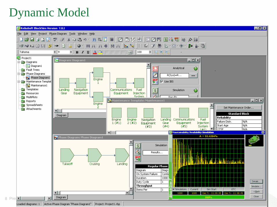
Dynamic Model

9 Presentation_name

Uses of the Model

• Design Phase

– Model is a simple “what if” tool for evaluating performance to compare the projected system reliability with the customer’s expectations.

• Operational Phase

– Validate model parameters with measured performance. Are you getting what you expected?

– If not, questions to ask include, was the system:

• Designed wrong

• Built wrong

• Installed wrong

• Operated wrong

• Maintained wrong

• In a “sick” location

10 Presentation_name

• Lognormal Distribution

• Weibull Distribution

Time Distributions (Models) of the Failure Rate Function

• Exponential Distribution

• Normal Distribution

-( ) tf t e

2

2

( - )-

21

( )2

t

f t e

2

2

(ln - )-

21

( )2

t

f t et

-1-

( )

tt

f t e

Very commonly used, even in cases to

which it does not apply (simple);

Applications: Electronics, mechanical

components etc.

Very straightforward and widely used;


components etc.

Very powerful and can be applied to

describe various failure processes;

Applications: Electronics, material,

structure etc.

Very powerful and can be applied to

describe various failure processes;


components, material, structure etc.


Exponential Model

• Definition: Constant Failure Rate

( )e( | ) ( | ) ( )

t xx

r tR x t P T t x T t e R x

e

( ) exp( ) 0, 0f t t t

( ) exp( ) 1 ( )R t t F t

( ) ( ) / ( )t f t R t

l(t)

t


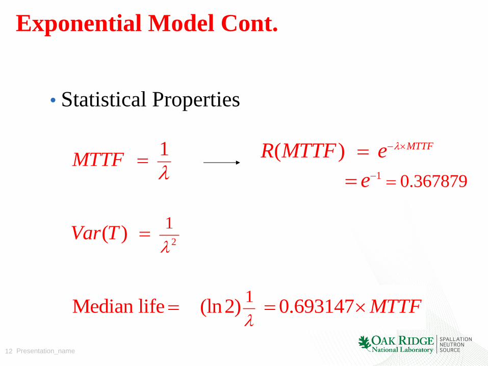
Exponential Model Cont.

1 0.367879

( ) MTTFR MTTF e

e

1MTTF

2

1( )Var T

1Median life (ln2) 0.693147 MTTF

• Statistical Properties


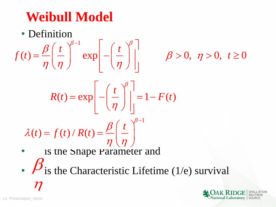
1

( ) exp 0, 0, 0t t

f t t

Weibull Model

• Definition

• is the Shape Parameter and

• is the Characteristic Lifetime (1/e) survival

1

( ) ( ) / ( )t

t f t R t

( ) exp 1 ( )t

R t F t


Weibull Model Continued:

1/

0

1(1 )tMTTF t e dt

2

2 2 1(1 ) (1 )Var

1/Median life ((ln2) )

• Statistical Properties


Versatility of Weibull Model

1

( ) ( ) / ( )t

t f t R t

Failure Rate:

Time t

1

Constant Failure Rate

Region

Fail

ure

Rate

0

Early Life

Region

0 1

Wear-Out

Region

1

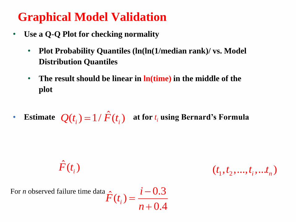
Graphical Model Validation

• Use a Q-Q Plot for checking normality

• Plot Probability Quantiles (ln(ln(1/median rank)/ vs. Model

Distribution Quantiles

• The result should be linear in ln(time) in the middle of the

plot

• Estimate at for ti using Bernard’s Formula

ˆ ( )iF t

0.3ˆ ( )0.4

i

iF t

n

For n observed failure time data

1 2( , ,..., ,... )i nt t t t

ˆ( ) 1/ ( )i iQ t F t


Example: Q-Q of Weibull Distribution and Weibull Fit (works well)

• T~Weibull(1, 4000) Generate 50 data points

10-5

100

105

0.01

0.02

0.05

0.10

0.25

0.50

0.75

0.90 0.96 0.99

Data

Pro

bab

ility

Weibull Probability Plot

0.632

1-e-1


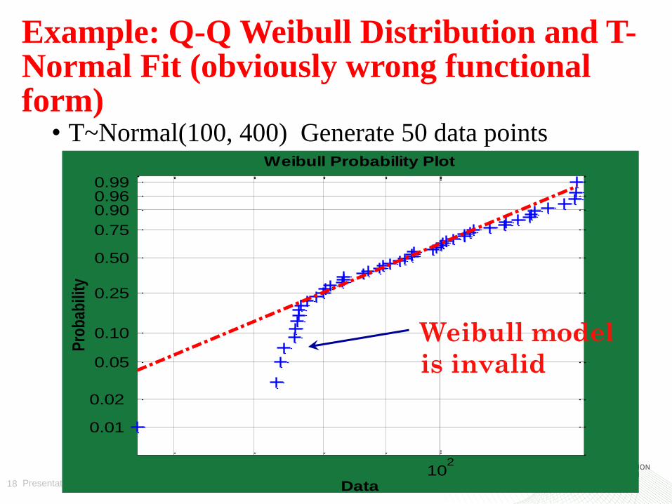
Example: Q-Q Weibull Distribution and T-Normal Fit (obviously wrong functional form)

• T~Normal(100, 400) Generate 50 data points

102

0.01

0.02

0.05

0.10

0.25

0.50

0.75

0.90 0.96 0.99

Data

Pro

bab

ility

Weibull Probability Plot

Weibull model

is invalid


Analysis of the Failure Rate of Systems or Components

With a relatively modest failure data set you can:

– Determine what your failure rate is at any given time

– Watch this rate change with time, through Infant Failures and into Random Failures

– Predict the onset of Terminal Failures

– Alerts you to watch more closely for the predictive symptoms of failure

– Determine the cost-effectiveness of proactive replacement before failure occurs

– Closely watch your Spares (number of spares, time to repair or acquire replacements, cost)


Weibull in Excel

http://www.qualitydigest.com/jan99/html/body_weibull.html


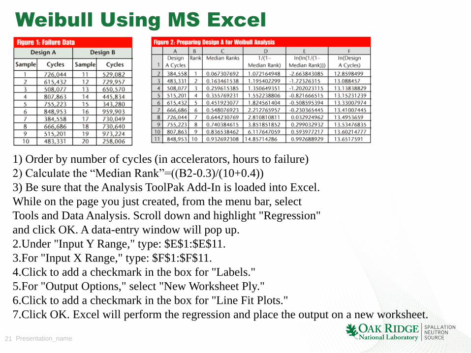
Weibull Using MS Excel

1) Order by number of cycles (in accelerators, hours to failure)

2) Calculate the “Median Rank”=((B2-0.3)/(10+0.4))

3) Be sure that the Analysis ToolPak Add-In is loaded into Excel.

While on the page you just created, from the menu bar, select

Tools and Data Analysis. Scroll down and highlight "Regression"

and click OK. A data-entry window will pop up.

2.Under "Input Y Range," type: $E$1:$E$11.

3.For "Input X Range," type: $F$1:$F$11.

4.Click to add a checkmark in the box for "Labels."

5.For "Output Options," select "New Worksheet Ply."

6.Click to add a checkmark in the box for "Line Fit Plots."

7.Click OK. Excel will perform the regression and place the output on a new worksheet.

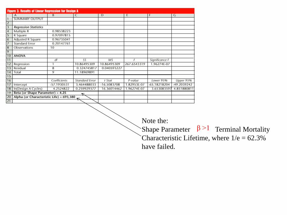
Note the:

Shape Parameter Terminal Mortality

Characteristic Lifetime, where 1/e = 62.3%

have failed.

β ˃1


SNS RF High Voltage Converter Modulator 2008 CCL1

hours to

failure Rank Median Ranks

1/(1-Median

Rank)

ln(ln(1/(1-

Median

Rank)))

ln(Design A

Cycles)

0.75 1 0.067307692 1.072164948 -2.66384309 -0.28768207

0.9 2 0.163461538 1.195402299 -1.72326315 -0.10536052

20.3 3 0.259615385 1.350649351 -1.20202312 3.01062089

73.4 4 0.355769231 1.552238806 -0.82166652 4.29592394

91.8 5 0.451923077 1.824561404 -0.50859539 4.5196123

97.2 6 0.548076923 2.212765957 -0.23036544 4.57677071

578.9 7 0.644230769 2.810810811 0.032924962 6.36112975

609.2 8 0.740384615 3.851851852 0.299032932 6.41214662

912.2 9 0.836538462 6.117647059 0.593977217 6.81585926

2115 10 0.932692308 14.85714286 0.992688929 7.65681009

SUMMARY OUTPUT

Regression Statistics

Multiple R 0.969525286

R Square 0.93997928

Adjusted R Square 0.93247669

Standard Error 0.289744238

Observations 10

ANOVA

df SS MS F Significance F

Regression 1 10.51808512 10.51808512 125.2873043 3.63718E-06

Residual 8 0.671613788 0.083951723

Total 9 11.18969891

Coefficients Standard Error t Stat P-value Lower 95% Upper 95% Lower 95.0% Upper 95.0%

Intercept -2.217586473 0.176953141 -12.53205486 1.53932E-06 -2.625641148 -1.809531798 -2.625641148 -1.809531798

ln(Design A Cycles) 0.391732899 0.034997459 11.19318115 3.63718E-06 0.311028614 0.472437184 0.311028614 0.472437184

Beta (or Shape Parameter) = 0.391732899

Alpha (or Characteristic Life) = 287.4260525

RESIDUAL OUTPUT

Observation Predicted ln(ln(1/(1-Median Rank))) Residuals

1 -2.330281006 -0.33356208

2 -2.258859654 0.535596503

3 -1.038227226 -0.16379589

4 -0.534731736 -0.286934779

5 -0.447105645 -0.061489749

6 -0.424714814 0.194349369

7 0.274277326 -0.241352364

8 0.294262312 0.00477062

9 0.452409836 0.141567381

10 0.781837942 0.210850988

-3

-2

-1

0

1

2

-5 0 5 10ln(l

n(1

/(1

-Med

ian

Ran

k))

)

ln(Design A Cycles)

ln(Design A Cycles) Line

Fit Plot

Beta =0.39 (Infant Failures)

Alpha = 287

Adjusted R square =0.93

The λ for an Exponential model = 475!!


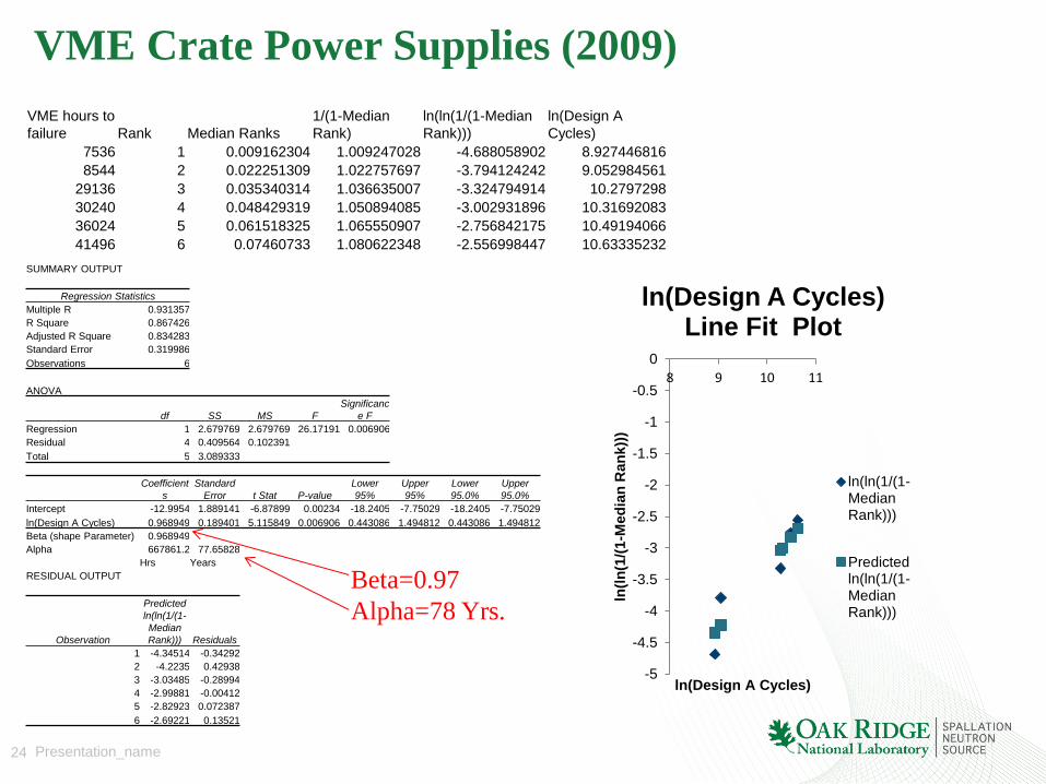
VME Crate Power Supplies (2009)

VME hours to

failure Rank Median Ranks

1/(1-Median

Rank)

ln(ln(1/(1-Median

Rank)))

ln(Design A

Cycles)

7536 1 0.009162304 1.009247028 -4.688058902 8.927446816

8544 2 0.022251309 1.022757697 -3.794124242 9.052984561

29136 3 0.035340314 1.036635007 -3.324794914 10.2797298

30240 4 0.048429319 1.050894085 -3.002931896 10.31692083

36024 5 0.061518325 1.065550907 -2.756842175 10.49194066

41496 6 0.07460733 1.080622348 -2.556998447 10.63335232

SUMMARY OUTPUT

Regression Statistics

Multiple R 0.931357

R Square 0.867426

Adjusted R Square 0.834283

Standard Error 0.319986

Observations 6

ANOVA

df SS MS F

Significanc

e F

Regression 1 2.679769 2.679769 26.17191 0.006906

Residual 4 0.409564 0.102391

Total 5 3.089333

Coefficient

s

Standard

Error t Stat P-value

Lower

95%

Upper

95%

Lower

95.0%

Upper

95.0%

Intercept -12.9954 1.889141 -6.87899 0.00234 -18.2405 -7.75029 -18.2405 -7.75029

ln(Design A Cycles) 0.968949 0.189401 5.115849 0.006906 0.443086 1.494812 0.443086 1.494812

Beta (shape Parameter) 0.968949

Alpha 667861.2 77.65828

Hrs Years

RESIDUAL OUTPUT

Observation

Predicted

ln(ln(1/(1-

Median

Rank))) Residuals

1 -4.34514 -0.34292

2 -4.2235 0.42938

3 -3.03485 -0.28994

4 -2.99881 -0.00412

5 -2.82923 0.072387

6 -2.69221 0.13521

-5

-4.5

-4

-3.5

-3

-2.5

-2

-1.5

-1

-0.5

0

8 9 10 11

ln(l

n(1

/(1

-Med

ian

Ran

k))

)

ln(Design A Cycles)

ln(Design A Cycles) Line Fit Plot

ln(ln(1/(1-MedianRank)))

Predictedln(ln(1/(1-MedianRank)))

Beta=0.97

Alpha=78 Yrs.


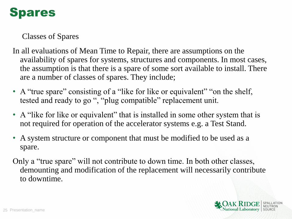
Spares

Classes of Spares

In all evaluations of Mean Time to Repair, there are assumptions on the availability of spares for systems, structures and components. In most cases, the assumption is that there is a spare of some sort available to install. There are a number of classes of spares. They include;

• A “true spare” consisting of a “like for like or equivalent” “on the shelf, tested and ready to go “, “plug compatible” replacement unit.

• A “like for like or equivalent” that is installed in some other system that is not required for operation of the accelerator systems e.g. a Test Stand.

• A system structure or component that must be modified to be used as a spare.

Only a “true spare” will not contribute to down time. In both other classes, demounting and modification of the replacement will necessarily contribute to downtime.


Spares

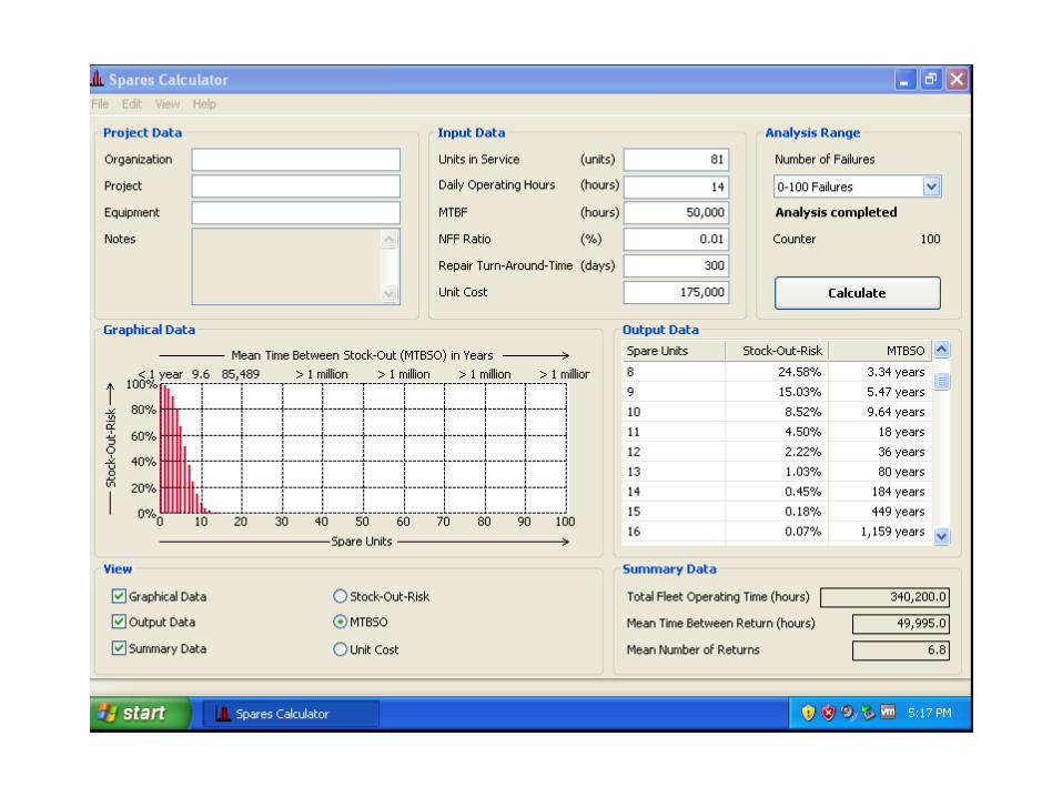
Beyond the “larger of 10% or 2” rule of thumb, the evaluation of the baseline number of spares should include a calculational basis which considers:

1. Number of installed units

2. Mean Time Between Failures (estimated at first, then validated against experience)

3. Mean Time to Repair or Replace in the calculation.

The result will be a Mean Time to Out of Stock as a function of the number of spare units.

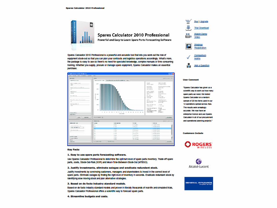
– Spares Calculator code is available – validated against MIL Spec - U.S. Navy, Reliability Engineering Handbook, NAVAIR 01-1A-32


Spares – How Many

• Use the MTBSO to evaluate what Comfort Level you can afford to have.

• Caveat –

– This calculation assumes a random distribution and is not accurate for NEW systems where a large number of identical are all installed at the same time.


Summary:

For a given set of performance data and an appropriate

model, analysis of the data can accurately yield MTBF,

MTTR for components and systems . The analysis can also

yield information on where components and systems are in

the lifetime curve so that you can make decisions about

when to replace components and how many you should

have in inventory (particularly important in long-lead-time

components).

These data can be used to validate your RAMI Model of

your accelerator systems.


Issues in Modeling

• “… no model is absolutely correct. In particular, however, some models are more useful than others.” –

• The model should be sufficiently simple to be handled by available mathematical and statistical methods, and be sufficiently realistic such that the deducted results are of practical use.


Backup Slides


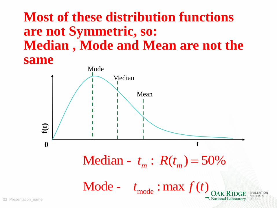
Most of these distribution functions are not Symmetric, so: Median , Mode and Mean are not the same

modeMode - : max ( )t f t

Median - : ( ) 50%m mt R t

f(t)

0 t

Mode

Median

Mean


Example of a Non-Constant Failure Rate Curve: The “Bathtub” Curve

Time t

1

Early Life

Region

2


Region

3

Wear-Out

Region

Fail

ure

Rate

0


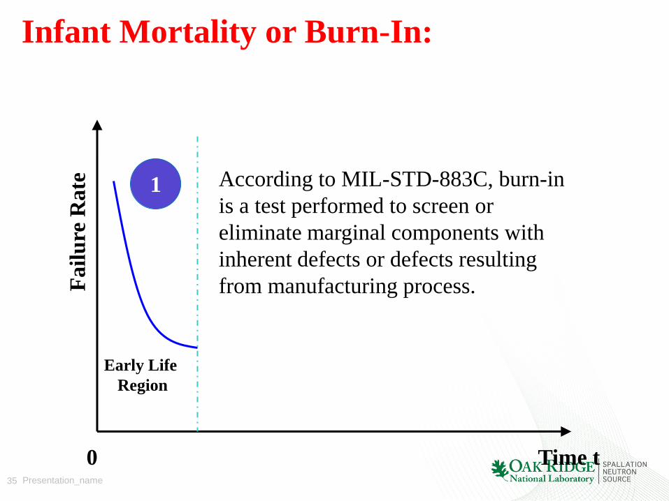
Infant Mortality or Burn-In:

Time t

1

Early Life

Region

Fail

ure

Rate

0

According to MIL-STD-883C, burn-in

is a test performed to screen or

eliminate marginal components with

inherent defects or defects resulting

from manufacturing process.


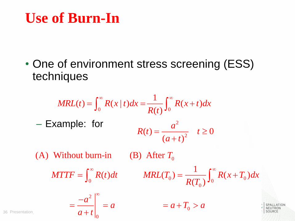
Use of Burn-In

• One of environment stress screening (ESS) techniques

– Example: for

0 0

1( ) ( | ) ( )

( )MRL t R x t dx R x t dx

R t

2

2( ) 0

( )

aR t t

a t

0

0 00 0

0

2

0

0

(A) Without burn-in (B) After

1 ( ) ( ) ( )

( )

T

MTTF R t dt MRL T R x T dxR T

aa a T a

a t


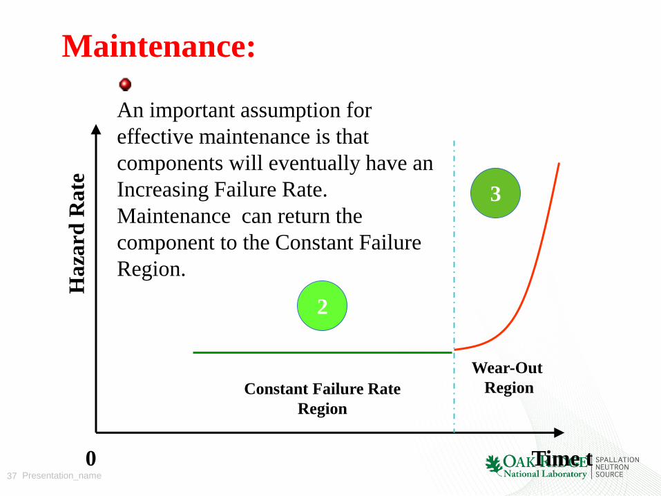
Maintenance:

Time t

3

Wear-Out

Region

Ha

zard

Rate

0

An important assumption for

effective maintenance is that

components will eventually have an

Increasing Failure Rate.

Maintenance can return the

component to the Constant Failure

Region.

2


Region

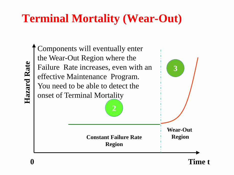
Terminal Mortality (Wear-Out)

Time t

3

Wear-Out

Region

Ha

zard

Rate

0

Components will eventually enter

the Wear-Out Region where the

Failure Rate increases, even with an

effective Maintenance Program.

You need to be able to detect the

onset of Terminal Mortality

2


Region


Exponential Distribution (Model)


Single/Multiple Failure Modes


Example

• The higher the failure rate is, the faster the reliability drops with time

l increases


Weibull Distribution (Model) and Model Validation

• Waloddi Weibull, a Swedish inventor and engineer invented

the Weibull distribution in 1937. The U.S. Air Force

recognized the merit of Weibull’s methods and funded his

research to 1975.

• Leonard Johnson at General Motors improved Weibull’s

methods. He suggested the use of median rank values for

plotting.

• The engineers at Pratt & Whitney found that the Weibull

method worked well with extremely small samples, even for 2

or 3 failures.

Background of Weibull


• Failure Probability Density is related to the Failure Probability by:

• Reliability Function is related to the Failure Probability Density by:

0

( ) ( )

x

f x f s ds ( ( ))

( )d F x

f xdx

( ) 1 ( ) ( ) t

R t F t f u du

1

2 2 is better than 1?


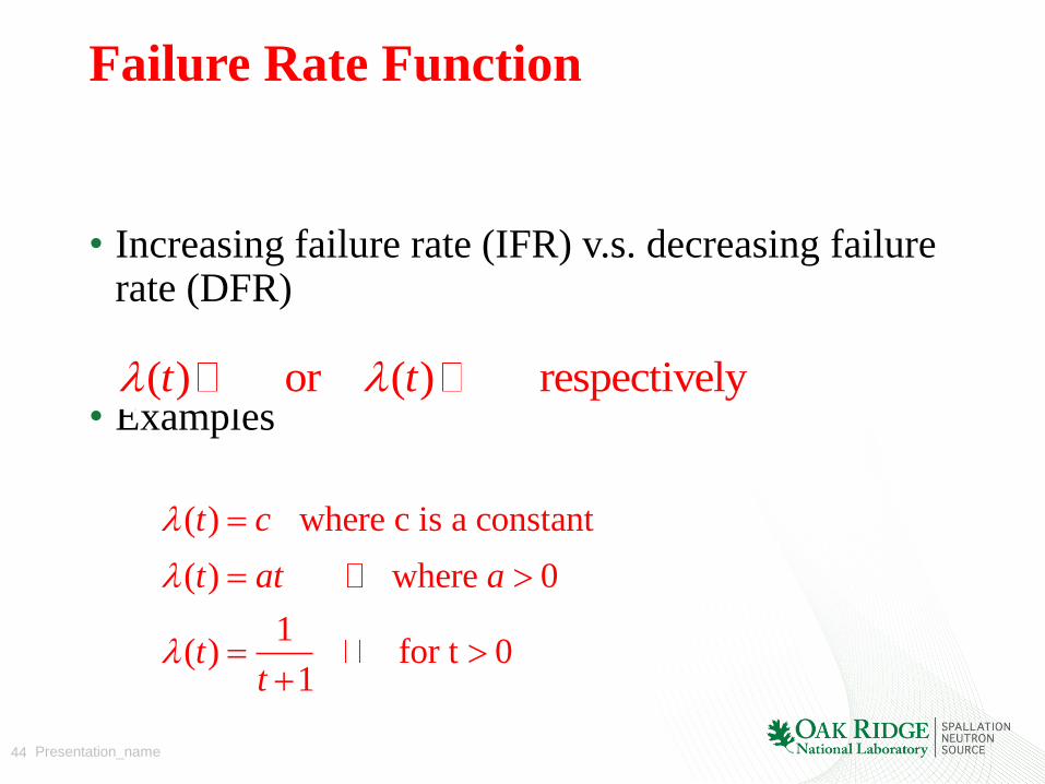
Failure Rate Function

• Increasing failure rate (IFR) v.s. decreasing failure rate (DFR)

• Examples ( ) or ( ) respectivelyt t

( ) where c is a constant

( ) where 0

1( ) for t 0

1

t c

t at a

tt


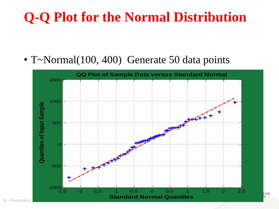
Q-Q Plot for the Normal Distribution

• T~Normal(100, 400) Generate 50 data points

-2.5 -2 -1.5 -1 -0.5 0 0.5 1 1.5 2 2.5-1000

-500

0

500

1000

1500

Standard Normal Quantiles

Qu

antil

es o

f In

pu

t Sam

ple

QQ Plot of Sample Data versus Standard Normal


Formal Statistical Test Procedures

2

• Test for assumption in a more statistical

way

• Goodness-of-Fit test

• Bartlett’s test for Exponential

• Mann’s test for Weibull

•Komogorov-Smirnov (KS) test


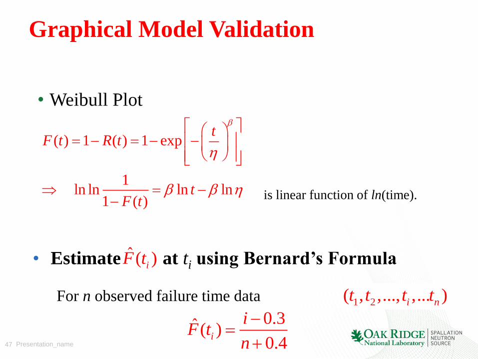
Graphical Model Validation

• Weibull Plot

( ) 1 ( ) 1 exp

1 ln ln ln ln

1 ( )

tF t R t

tF t

ˆ ( )iF t

is linear function of ln(time).

• Estimate at ti using Bernard’s Formula

0.3ˆ ( )0.4

i

iF t

n

For n observed failure time data 1 2( , ,..., ,... )i nt t t t

practical applications of reliability theory -...

Documents