power system dynamics prof. m. l. kothari department of...

Power System Dynamics

Prof. M. L. Kothari

Department of Electrical Engineering

Indian Institute of Technology, Delhi

Lecture - 05

The Equal Area Criterion for Stability

(Refer Slide Time: 00:55)

Friends today, we shall discuss ah the equal area criteria for stability.


We have studied that to analyze the stability of a power system, we have to solve swing

equations and solution of swing equations is through a numerical technique and it is a

time consuming process. The equal area criteria of stability is very powerful tool to

understand the basic concepts of stability. However, as we will see that this criteria has

its limited applications.

Now, today in our study we will establish this basic concepts pertaining to equal area

criteria and we will analyze considering a one machine swinging with respect to the

infinite bus, then we will develop the equivalent of one machine infinite bus system of a

2 machine system.


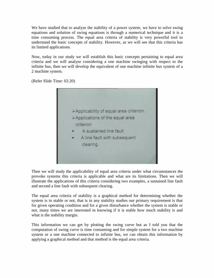
Then we will study the applicability of equal area criteria under what circumstances the

provoke systems this criteria is applicable and what are its limitations. Then we will

illustrate the applications of this criteria considering two examples, a sustained line fault

and second a line fault with subsequent clearing.

The equal area criteria of stability is a graphical method for determining whether the

system is in stable or not, that is in any stability studies our primary requirement is that

for given operating condition and for a given disturbance whether the system is stable or

not, many times we are interested in knowing if it is stable how much stability is and

what is the stability margin.

This information we can get by plotting the swing curve but as I told you that the

computation of swing curve is time consuming and for simple system for a two machine

system or a one machine connected to infinite bus, we can obtain this information by

applying a graphical method and that method is the equal area criteria.



Now when this criteria is applicable, its use wholly or partially eliminates the need of

computing swing curve and thus saves considerable amount of time. I am emphasizing

here, that it eliminates the computation of swing curve wholly or partially. Okay that we

will see actually when we attempt some example.

This criteria is applicable to any two machine system for which commonly made

assumptions are applicable right. We have studied the commonly made assumptions for

analyzing the transient stability problem and when these assumptions are applicable, this

can be applied to any two machine system.


Now first we will mathematically establish the equal area criteria of stability to establish

we start with the swing equation of a machine, here we are considering a machine

connected to the infinite bus, infinite bus is one which can be represented by a constant

voltage source its internal impedance is 0 and its inertia is infinite. Now you multiply this

both sides of this equation by a term 2 delta d delta by dt.


When we multiply both the sides by this term 2 times d delta by dt, we get equation in

this form 2 times d square

delta by dt square into d delta by dt equal to 2 times Pa by M, d

delta by dt. Now this left hand side of this equation can be identified as derivative of d

delta by dt square, you look it very carefully that is if you take this term and find out its

derivative you will get the term 2 times d square delta by dt

square d delta by dt, okay

and right hand side we are writing as it is 2 times Pa by M d delta by dt okay.


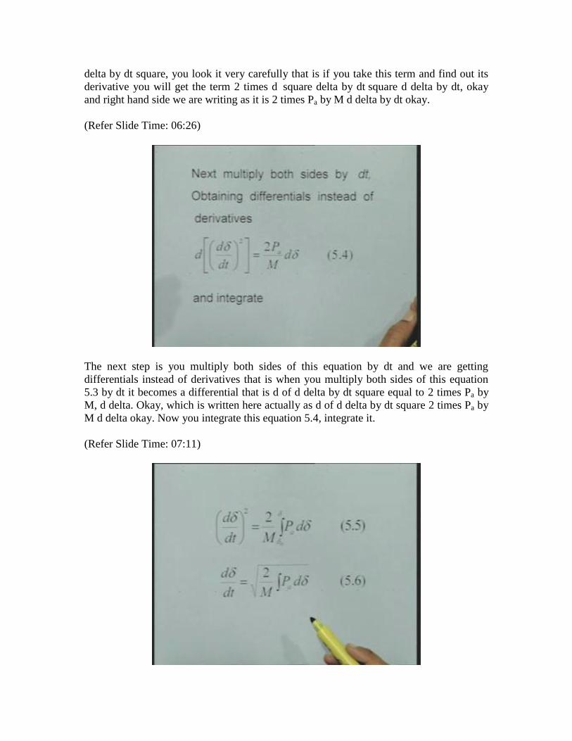
The next step is you multiply both sides of this equation by dt and we are getting

differentials instead of derivatives that is when you multiply both sides of this equation

5.3 by dt it becomes a differential that is d of d delta by dt square equal to 2 times Pa by

M, d delta. Okay, which is written here actually as d of d delta by dt square 2 times Pa by

M d delta okay. Now you integrate this equation 5.4, integrate it.


When you integrate, you will get d delta by dt square equal to 2 by M integral Pa d delta.

This integration we are doing over certain range of delta that is start with initial value of

delta naught delta equal to delta naught and go to some value of delta. I am just putting it

general that is delta naught to delta, I am not specifying what should be the value of delta

here.

Now from this equation 5.5, we can write d delta by dt equal to square root of 2 by M

integral Pa d delta, the limits are implied okay. Now we look at this equation and we

know that the condition which indicates the stability of the system is that d delta by dt

should be 0 that is a system starts where it is perturbed right with the initial value delta

naught and when it is, when delta increases it will attain a maximum value then start

decreasing that is the condition of stability, it means that when it goes to maximum and

start decreasing that maximum point, at that maximum point d delta by dt is 0 therefore,

the condition to indicate the stability is that d delta dt should become 0.


Now for this d delta by dt2 become 0 which is the condition to indicate the stability of the

system, our requirement is that the integral of Pa d delta from a initial value of delta equal

to delta naught to some value of delta m should be 0 that is if I, if I plot the area under the

curve Pa that is accelerating power starting from initial value of delta equal to delta

naught to some maximum value of delta m and in case the in the area under this curve is

0 right, then at the value of delta equal to delta m the d delta by dt will become 0 right.


Now this I will show here in this diagram, this is the power angle characteristic of the

system, this was the mechanical input line. Now in this diagram I am simply showing that

suppose initially the system was operating at delta naught and the power angle

characteristic applicable for the initial operating condition was not this but something

different. The moment fault occurs on the system the operating point has shifted from this

point to this point okay then delta will increase from initial operating from the point a on

the power angle curve Pe.

The initial acceleration is given by this or initial accelerating power is given by this line,

this is the initial accelerating power, okay therefore rotor accelerates when rotor

accelerates the delta will increase, speed increases then delta increases and now when it

reaches the point b right, the accelerating power becomes 0. Now at this point what is the

rotor speed?

The rotor speed is more than the synchronous speed because, because from when it is

travels from this point a to b, the rotor is accelerated gain some kinetic energy it has

gained some extra speed over and above the synchronous speed therefore, at this point

the rotor will not stop it will continue to, the angle will continue to increase. Now the

moment it crosses this point b we see that the accelerating power becomes negative that

electrical power output becomes more than the mechanical input.

Therefore, now the rotor will be subjected to retardation and when it reaches the point c

point c, if suppose whatsoever the kinetic energy it has gained if it is return back or is ah

lost then at point c the rotor will again attain a speed equal to synchronous speed and

therefore for the system to be stable, the rotor will swing from delta naught to delta m and

the area under the accelerating power.

Now here the accelerating power is obtained by separating therefore here I can say that

accelerating power curve is given by this difference, okay and therefore this area should

be 0. Now for this area under the accelerating power curve to become 0 requires that the

this this positive area, we call this as a positive area because accelerating power is

positive this is called negative area, the accelerating power is negative therefore these 2

areas should be equal and this is what is known as the equal area criteria of stability. Now

this equal area criteria of stability can also be interpreted in terms of the kinetic energy

gain and kinetic energy lost right.



Now we know actually that suppose a rotor is subjected to a torque T, torque T and when

it swings from delta naught to delta the, the work done on the rotor is equal to or work

done by the rotating body is equal to T into d delta. This is actually when the delta is

small and you integrate this expression from delta naught to sum value delta then this

becomes the work done when the rotating body accelerates, okay or decelerates it

depends upon the situation and hence we can say that the area a1 represents kinetic

energy gained by this machine or I can say this area a1 is directly proportional to kinetic

energy gained there has to be some proportionality constant I cannot say that a1 is in in

joules or mega joules or so it will depend upon what is the unit which we have attached to

it.

Now the derivation is which we have seen just now is considering a machine connected

to infinite bus. Now suppose you have 2 finite machines, 2 finite machines a problem that

of a synchronous generator supplying power to a synchronous motor through a

transmission line. Then this 2 finite machine system can be replaced by an equivalent

machine infinite bus system, this derivation is very straight forward we take the swing

equation of machine 1, d square delta 1 by dt

square equal to Pa1 by M1 that is Pm1 minus

P1 by M1. Then we take a swing equation of second machine ah d2 delta 2 by dt equal to

Pa2 by M2 that is Pa2 is Pm2 minus P21 okay.


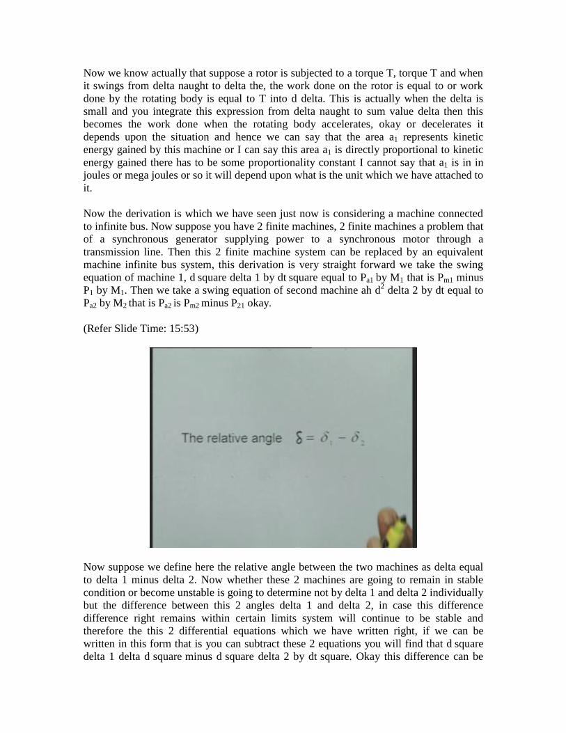
Now suppose we define here the relative angle between the two machines as delta equal

to delta 1 minus delta 2. Now whether these 2 machines are going to remain in stable

condition or become unstable is going to determine not by delta 1 and delta 2 individually

but the difference between this 2 angles delta 1 and delta 2, in case this difference

difference right remains within certain limits system will continue to be stable and

therefore the this 2 differential equations which we have written right, if we can be

written in this form that is you can subtract these 2 equations you will find that d square

delta 1 delta d square

minus d

square delta 2 by dt

square. Okay this difference can be

written as d square delta by dt

square because delta 1 minus delta 2 is delta and on this

right hand side you have Pa1 by M1 minus Pa2 by M2.



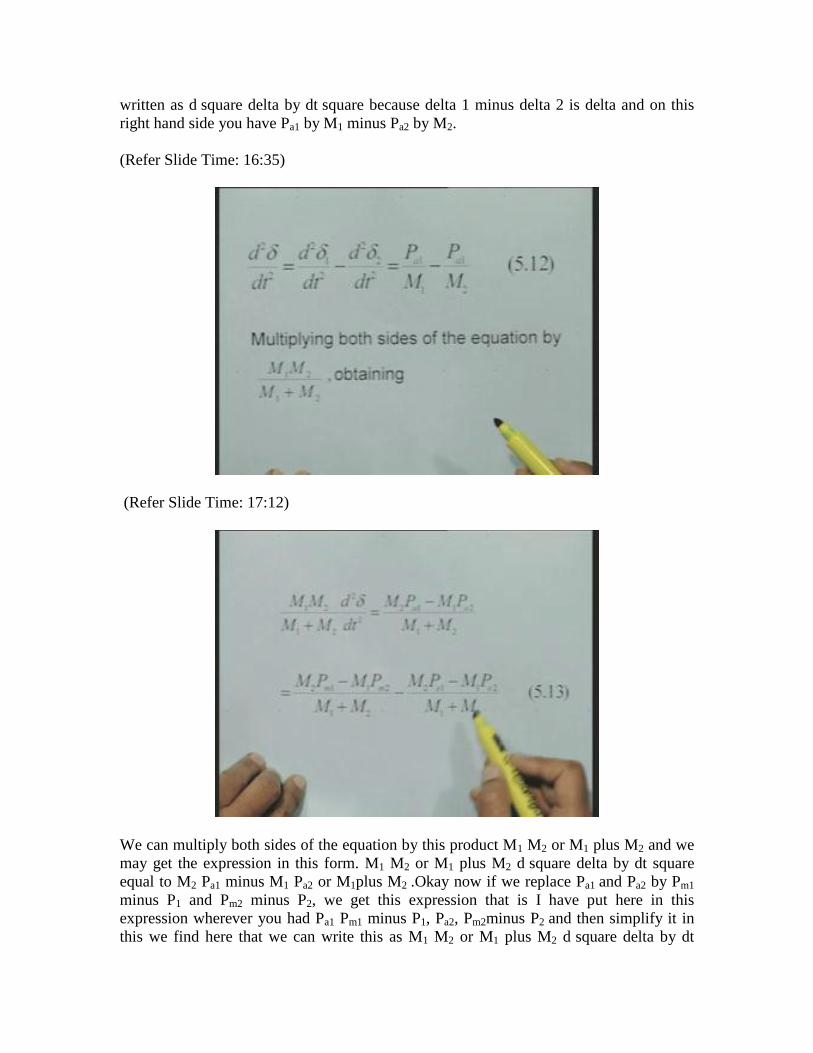
We can multiply both sides of the equation by this product M1 M2 or M1 plus M2 and we

may get the expression in this form. M1 M2 or M1 plus M2 d square delta by dt square

equal to M2 Pa1 minus M1 Pa2 or M1plus M2 .Okay now if we replace Pa1 and Pa2 by Pm1

minus P1 and Pm2 minus P2, we get this expression that is I have put here in this

expression wherever you had Pa1 Pm1 minus P1, Pa2, Pm2minus P2 and then simplify it in

this we find here that we can write this as M1 M2 or M1 plus M2 d square delta by dt

square equal to M2 Pm1 minus M1 Pm2 divided by M1plus M 2,that is in this term we have

the inertia constants and mechanical powers while here in this term we have inertia

constants and electrical powers P1 minus P1 and P2 okay.

Now this equation may be considered to be the swing equation of a machine connected to

infinite bus, where where the equivalent inertia constant is M1M 2 or M 1 plus M2, the

equivalent mechanical input is given by this expression and equivalent electrical output is

given by this expression.



Therefore, we can say that this expression written as M times d2 delta by dt2 equal to Pa

Pm minus Pe, where Pm is given by this expression, Pe is given by this expression, we can

say that Pm is the equivalent mechanical input Pe is the equivalent electrical output and

the equivalent inertia constant is M1 M2 over M1 plus M2. Now at this point you can

understand that the equivalent inertia constant is as if we are connecting 2 resistances in

parallel to find out the equivalent resistance.


Suppose you have 2 resistances r1 and r2 and you put them in parallel the equivalent

resistance is r1, r2 or r 1 plus r2 therefore this is the equivalent inertia constant is primarily

determined by or is going to be closer to the smaller one that is suppose I put M1 M2 M

plus M2 values, if M2 is large as compared to M1. Okay then we will find out the value let

us say I will just take example take just values actually let us say M1 is 5 and M2 is say 50

what will be the resultant? It is going to be less than 5 but it is closer to 5 not closer to a

50 therefore, the equivalent machine will have the inertia which is less than, less than the

the inertia of a smaller machine or inertia of a machine which has a smaller inertia

constant.

Now here at this stage, to illustrate the application of equal area criteria for analyzing

stability of a system, I will consider an example, the example we consider is a simple

example. Let us consider this example, we have a synchronous generator connected to a

double circuit transmission line to an infinite bus, we put infinity here to show that it is

infinite bus its inertia constant is infinite. To illustrate the application of equal area

criteria of stability what we will consider is that yes there is a machine infinite bus

system. We will consider a fault at the middle of the transmission line, one of the

transmission lines at the point P.


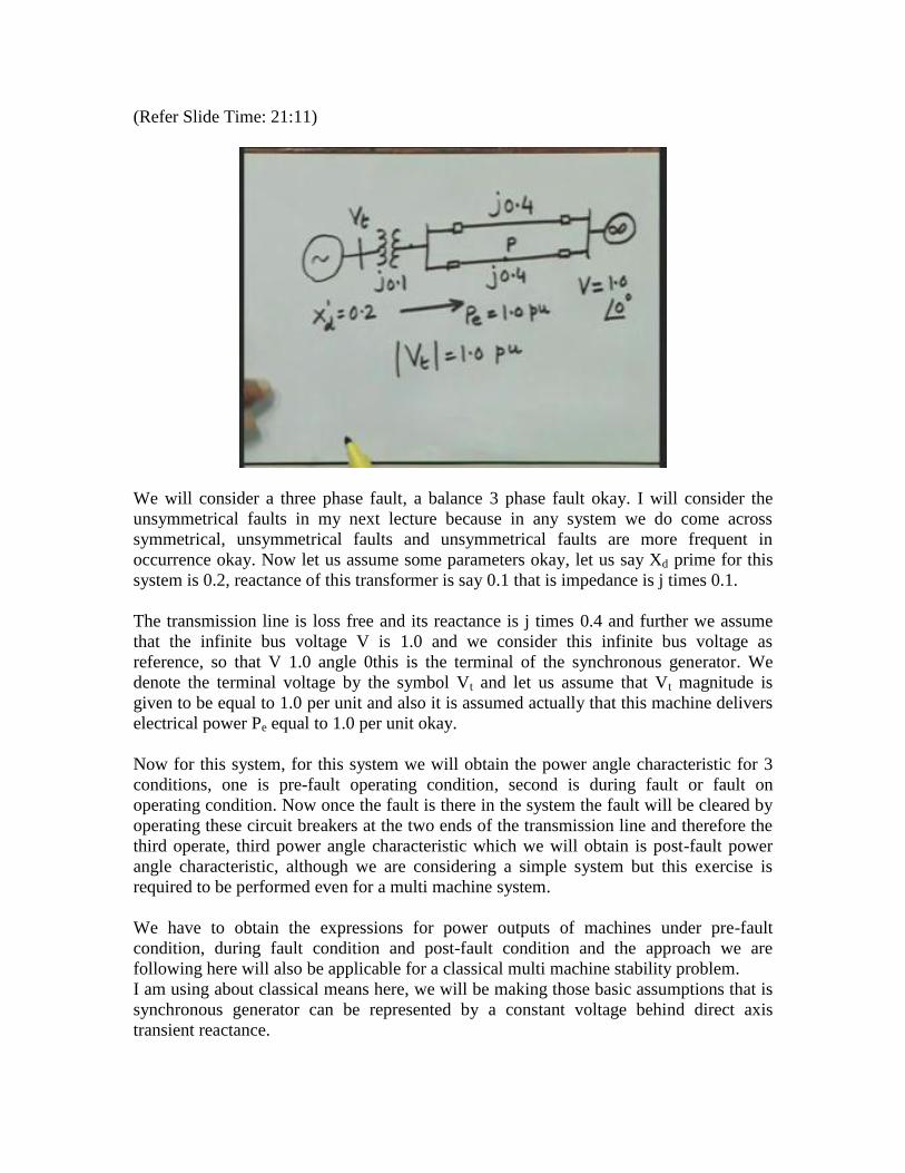
We will consider a three phase fault, a balance 3 phase fault okay. I will consider the

unsymmetrical faults in my next lecture because in any system we do come across

symmetrical, unsymmetrical faults and unsymmetrical faults are more frequent in

occurrence okay. Now let us assume some parameters okay, let us say Xd prime for this

system is 0.2, reactance of this transformer is say 0.1 that is impedance is j times 0.1.

The transmission line is loss free and its reactance is j times 0.4 and further we assume

that the infinite bus voltage V is 1.0 and we consider this infinite bus voltage as

reference, so that V 1.0 angle 0this is the terminal of the synchronous generator. We

denote the terminal voltage by the symbol Vt and let us assume that Vt magnitude is

given to be equal to 1.0 per unit and also it is assumed actually that this machine delivers

electrical power Pe equal to 1.0 per unit okay.

Now for this system, for this system we will obtain the power angle characteristic for 3

conditions, one is pre-fault operating condition, second is during fault or fault on

operating condition. Now once the fault is there in the system the fault will be cleared by

operating these circuit breakers at the two ends of the transmission line and therefore the

third operate, third power angle characteristic which we will obtain is post-fault power

angle characteristic, although we are considering a simple system but this exercise is

required to be performed even for a multi machine system.

We have to obtain the expressions for power outputs of machines under pre-fault

condition, during fault condition and post-fault condition and the approach we are

following here will also be applicable for a classical multi machine stability problem.

I am using about classical means here, we will be making those basic assumptions that is

synchronous generator can be represented by a constant voltage behind direct axis

transient reactance.

Now with this information given how to find out the pre-fault power angle characteristic

Therefore, here our primary requirement is that to get the pre-fault power angle

characteristic what do we need is the voltage behind transient reactance which is not

given, what is given is the voltage at the terminal of the machine. Now we can use this

information to compute, to compute ah pre-fault power angle what is first step is you

draw from the one line diagram a reactance diagram.



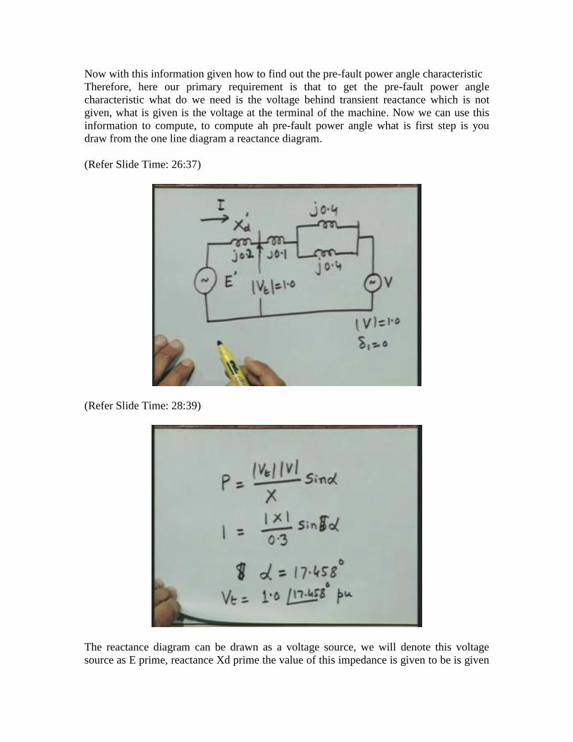
The reactance diagram can be drawn as a voltage source, we will denote this voltage

source as E prime, reactance Xd prime the value of this impedance is given to be is given

as j times 0.1, the transformer reactance is .1 per unit that its impedance is I am sorry, the

generator reactance is 0.2 not point .2 transformer is 0.1. These 2 transmission lines and

infinite bus voltage, we denote this as V at this point which is the terminal of the

synchronous generator the voltage is Vt and this magnitude of this voltage Vt is 1.0 while

this magnitude of V is 1.0 and delta 1 is taken as our delta is 0 the delta 1 is 0, okay. I can

call it delta, now the with this information or with this equivalent circuit what do we do is

we find out what is the phase angle of this Vt with respect to infinite bus voltage.

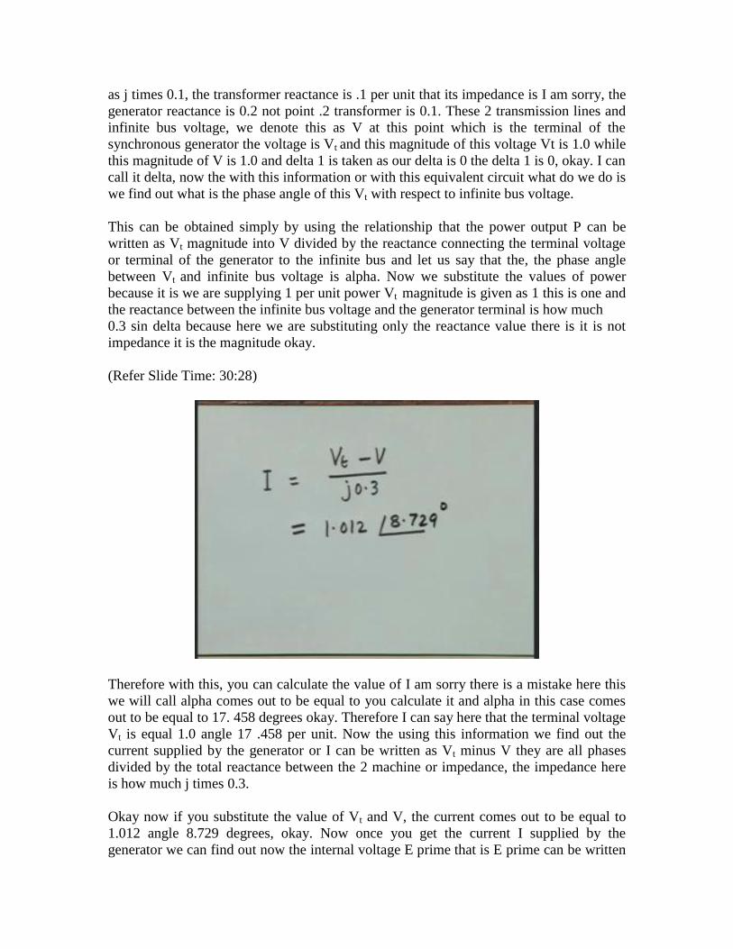
This can be obtained simply by using the relationship that the power output P can be

written as Vt magnitude into V divided by the reactance connecting the terminal voltage

or terminal of the generator to the infinite bus and let us say that the, the phase angle

between Vt and infinite bus voltage is alpha. Now we substitute the values of power

because it is we are supplying 1 per unit power Vt magnitude is given as 1 this is one and

the reactance between the infinite bus voltage and the generator terminal is how much

0.3 sin delta because here we are substituting only the reactance value there is it is not

impedance it is the magnitude okay.


Therefore with this, you can calculate the value of I am sorry there is a mistake here this

we will call alpha comes out to be equal to you calculate it and alpha in this case comes

out to be equal to 17. 458 degrees okay. Therefore I can say here that the terminal voltage

Vt is equal 1.0 angle 17 .458 per unit. Now the using this information we find out the

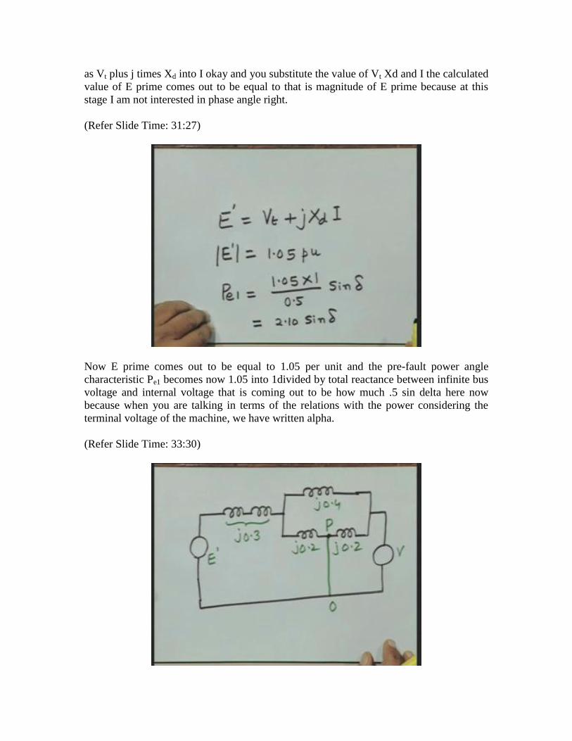
current supplied by the generator or I can be written as Vt minus V they are all phases

divided by the total reactance between the 2 machine or impedance, the impedance here

is how much j times 0.3.

Okay now if you substitute the value of Vt and V, the current comes out to be equal to

1.012 angle 8.729 degrees, okay. Now once you get the current I supplied by the

generator we can find out now the internal voltage E prime that is E prime can be written

as Vt plus j times Xd into I okay and you substitute the value of Vt Xd and I the calculated

value of E prime comes out to be equal to that is magnitude of E prime because at this

stage I am not interested in phase angle right.


Now E prime comes out to be equal to 1.05 per unit and the pre-fault power angle

characteristic Pe1 becomes now 1.05 into 1divided by total reactance between infinite bus

voltage and internal voltage that is coming out to be how much .5 sin delta here now

because when you are talking in terms of the relations with the power considering the

terminal voltage of the machine, we have written alpha.


Now delta is the angle and therefore the pre-fault power angle characteristic is now 2.10

sin, okay this these steps are extremely important. We will follow we may have to follow

the similar steps for a multi machine system also. The next step is we want to find out the

power angle curve or power angle characteristic when fault is on.

When the fault is on, on the system we can write down or we can again draw the

reactance diagram, since the I have consider the fault at the middle of the line therefore I

will divide this line reactance into 2 parts and show as .2 .2 on both the sides of the

faulted point or voltage at the point P.

Now since, we have considered a balanced three phase fault this P will be connected to

the reference bus directly connected there is no impedance involved however when we

consider the unsymmetrical fault we will see that to analyze the or to obtain the power

angle characteristic during fault conditions there will be some impedance connected

between the faulted point P and reference bus. This impedance will depend upon the type

of fault but for a 3 phase fault the impedance to be connected is 0.

Now here we are considering a three phase metallic fault okay there is no fault

impedance. Now in this the total reactance of the this these two components that is the

Xd prime and the transformer can be combined and this can be written as impedance is

0.3, this is j times 0.4, this is j times 0.2, this is j times 0.2 and this voltage is this voltage

magnitude is this is V voltage, this is E prime okay. Now what we do is we will try to

simply this network, so that we can find out the power angle characteristic during fault on

period.


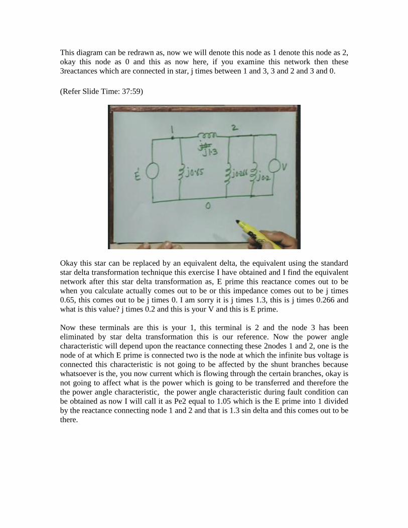
This diagram can be redrawn as, now we will denote this node as 1 denote this node as 2,

okay this node as 0 and this as now here, if you examine this network then these

3reactances which are connected in star, j times between 1 and 3, 3 and 2 and 3 and 0.


Okay this star can be replaced by an equivalent delta, the equivalent using the standard

star delta transformation technique this exercise I have obtained and I find the equivalent

network after this star delta transformation as, E prime this reactance comes out to be

when you calculate actually comes out to be or this impedance comes out to be j times

0.65, this comes out to be j times 0. I am sorry it is j times 1.3, this is j times 0.266 and

what is this value? j times 0.2 and this is your V and this is E prime.

Now these terminals are this is your 1, this terminal is 2 and the node 3 has been

eliminated by star delta transformation this is our reference. Now the power angle

characteristic will depend upon the reactance connecting these 2nodes 1 and 2, one is the

node of at which E prime is connected two is the node at which the infinite bus voltage is

connected this characteristic is not going to be affected by the shunt branches because

whatsoever is the, you now current which is flowing through the certain branches, okay is

not going to affect what is the power which is going to be transferred and therefore the

the power angle characteristic, the power angle characteristic during fault condition can

be obtained as now I will call it as Pe2 equal to 1.05 which is the E prime into 1 divided

by the reactance connecting node 1 and 2 and that is 1.3 sin delta and this comes out to be

there.


We computed and its value comes out to be 0.808 sin delta or what you observe here is

that this Pe2 which is the equal to Pe max into sin delta right, the the maximum value of this

power angle characteristic will depend primarily upon what is the reactance connecting

the internal voltage of the synchronous machine to the infinite bus voltage more is this

reactance less will be the voltage okay.

Now we can very easily obtain the post fault power angle characteristic under the post

fault condition one of the transmission line is cleared or it is removed and therefore the

reactance connecting the two nodes, internal voltage of the synchronous generator and

infiltrate bus voltage that comes out to be how much .7 therefore our characteristic is now

this divided by .7 sin delta. Okay now these are the 3 important power angle

characteristics which one has to compute or obtain for analyzing the stability of a

machine infinite bus system either we apply equal criteria or you directly solve the some

equation, it is the a material. The these 3 characteristics if you draw it can be shown like

this.

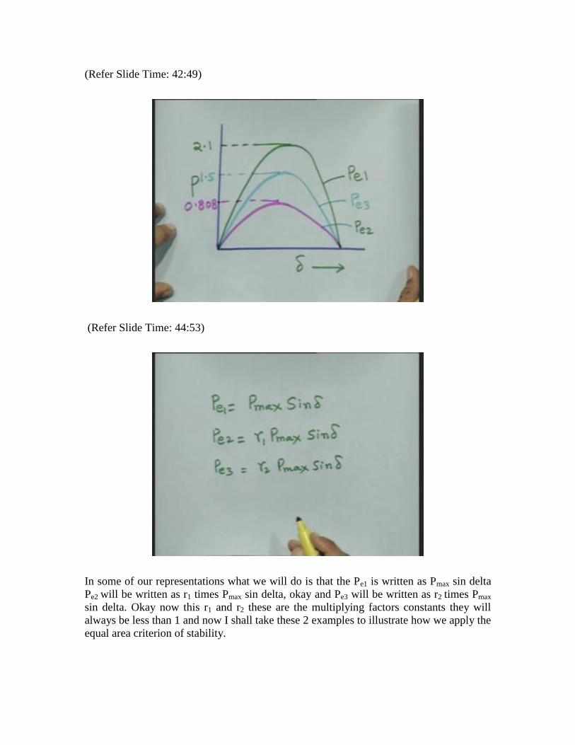
I will call this is a Pe1 this is pre-fault power angle characteristic in this particular case

this is 2.1, P maximum value under faulted condition or the power angle curve under

fault condition was found to have the maximum value equal to around .808 and therefore

the characteristic can be shown to be like this and this is 0.808 after the fault is cleared,

the amplitude of this power angle characteristic how much what is the value of this1.5,

1.5 that is very good and therefore the third characteristic can be plotted here, then this is

1.5 this is your Pe3, this is your Pe Pe2.



In some of our representations what we will do is that the Pe1 is written as Pmax sin delta

Pe2 will be written as r1 times Pmax sin delta, okay and Pe3 will be written as r2 times Pmax

sin delta. Okay now this r1 and r2 these are the multiplying factors constants they will

always be less than 1 and now I shall take these 2 examples to illustrate how we apply the

equal area criterion of stability.


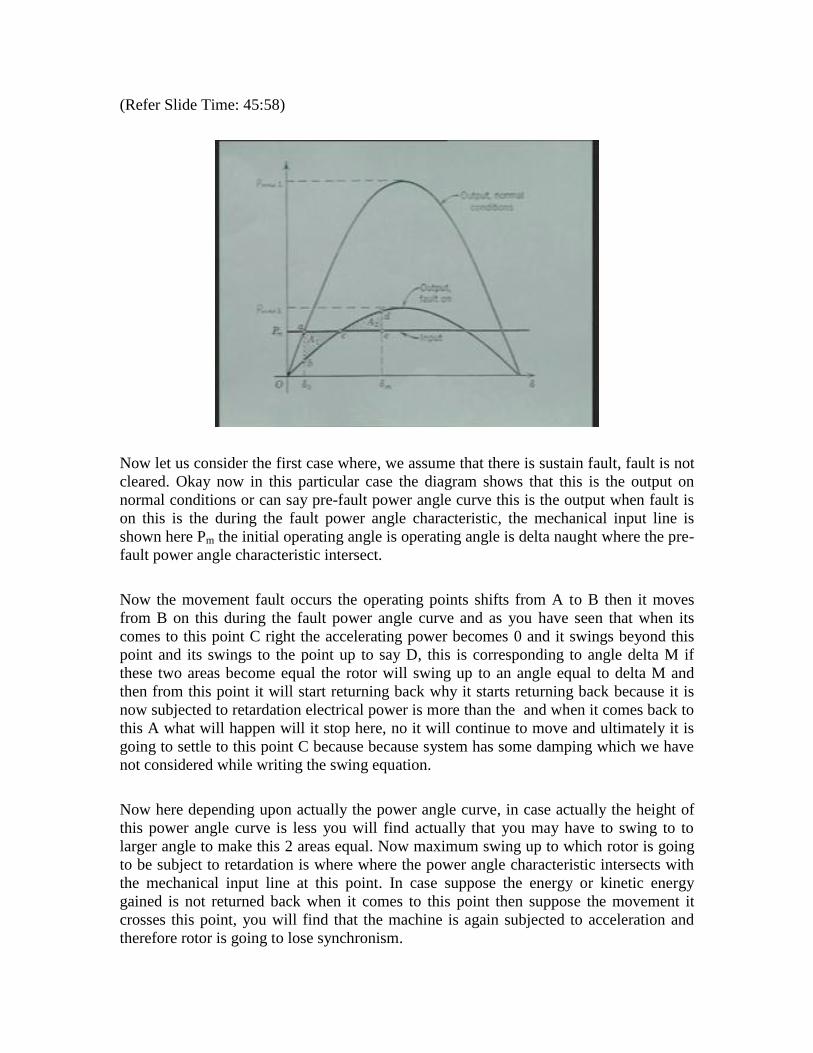
Now let us consider the first case where, we assume that there is sustain fault, fault is not

cleared. Okay now in this particular case the diagram shows that this is the output on

normal conditions or can say pre-fault power angle curve this is the output when fault is

on this is the during the fault power angle characteristic, the mechanical input line is

shown here Pm the initial operating angle is operating angle is delta naught where the pre-

fault power angle characteristic intersect.

Now the movement fault occurs the operating points shifts from A to B then it moves

from B on this during the fault power angle curve and as you have seen that when its

comes to this point C right the accelerating power becomes 0 and it swings beyond this

point and its swings to the point up to say D, this is corresponding to angle delta M if

these two areas become equal the rotor will swing up to an angle equal to delta M and

then from this point it will start returning back why it starts returning back because it is

now subjected to retardation electrical power is more than the and when it comes back to

this A what will happen will it stop here, no it will continue to move and ultimately it is

going to settle to this point C because because system has some damping which we have

not considered while writing the swing equation.

Now here depending upon actually the power angle curve, in case actually the height of

this power angle curve is less you will find actually that you may have to swing to to

larger angle to make this 2 areas equal. Now maximum swing up to which rotor is going

to be subject to retardation is where where the power angle characteristic intersects with

the mechanical input line at this point. In case suppose the energy or kinetic energy

gained is not returned back when it comes to this point then suppose the movement it

crosses this point, you will find that the machine is again subjected to acceleration and

therefore rotor is going to lose synchronism.



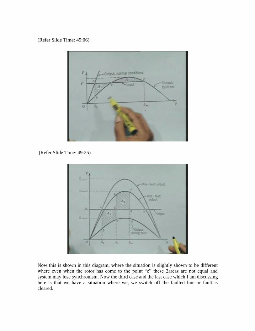
Now this is shown in this diagram, where the situation is slightly shown to be different

where even when the rotor has come to the point “e” these 2areas are not equal and

system may lose synchronism. Now the third case and the last case which I am discussing

here is that we have a situation where we, we switch off the faulted line or fault is

cleared.

Now you start looking at this there are 3 power angle curves this is the mechanical input

line initially we are operating at this point A, the movement fault occurs you shift to the

point B on the during the fault power angle curve. Now when you are moving on this

curve at this point C at on the angle equal to delta C the fault is cleared. We call this as a

fault clearing angle, the angle at which the fault is cleared then you will shift from this

point now to the post fault power angle curve then that is this is the, this curve is the post

fault output again as you know that this is this this is the area a1 that is this is bound by

these 2 angles and this power angle characteristic and mechanical input line this becomes

the accelerating area from “e” it will continue to swing it come to the point f and the

maximum angle becomes delta M at this point we find actually that these 2 areas equal

and therefore the maximum swing is up to delta M and the system will return back.

Now a new new stable operating point is now where the post fault power angle

characteristic intersects the mechanical input line that is in this diagram this is the new

stable operating point therefore, the rotor is going to swing around this point okay

oscillate around this point and because it has some damping, it will settle to this new

condition. Now with this I will just summarize what we have discussed today.

We have established the equal area criterion of stability. We have also obtained for a two

finite machine system an equivalent a machine infinite bus system. We have also

obtained for a given particular system the pre-fault, during fault and post fault power

angle characteristic a simple method is you can say discussed here and at the end I have

considered the 2 cases, one is considering a sustained fault and another is the fault cleared

after small amount of time, small time. Okay I conclude my presentation here and thank

you very much.

power system dynamics prof. m. l. kothari department of...

Documents