Power Spectral Analysis of a Multiscale Chaotic Dynamical System

SERGEI SOLDATENKO

Australian Center for Weather and Climate Research

700 Collins Street, Melbourne 3008

AUSTRALIA

s.soldatenko@bom.gov.au

Abstract: - In this paper, power spectral analysis of deterministic multiscale chaotic dynamical system is

presented. The system is obtained by coupling two versions of the well-known Lorenz (1963) model with

distinct time scales that differ by a certain time-scale factor. This system is commonly used for exploring

various aspects of atmospheric and climate dynamics, and also for estimating the computational effectiveness

of numerical schemes and algorithms used in numerical weather prediction, data assimilation and climate

simulation. The influence of the coupling strength parameter on power spectral densities and spectrogram is

discussed.

Key-Words: - Dynamical System, Deterministic Chaos, Power Spectral Density, Climate Modeling

1 Introduction Dynamical systems theory represents a powerful

framework for developing mathematical models of

the earth system and analyzing and exploring time

evolution of the earth’s system components [1, 2].

The “earth system” is a term that is commonly used

to refer to the interacting atmosphere, hydrosphere,

lithosphere, cryosphere and biosphere together with

numerous natural and anthropogenic physical,

chemical, and biological cycles of our planet. It is

important to note, that the dynamical system

concept is also widely used in environmental,

geophysical, biological and engineering sciences.

In the most general meaning, a hypothetical

dynamical system can be formally specified by its

state vector the coordinates of which (state or

dynamic variables) characterize exactly the state of

a system at any moment, and a well-defined

function (i.e. rule) which describes, given the

current state, the evolution with time of state

variables. There are two kinds of dynamical system:

continuous time and discrete time. Continuous-time

dynamical systems are commonly specified by a set

of ordinary or partial differential equations and the

problem of the evolution of state variables in time is

then considered as an initial value problem.

However, with respect to the earth system

simulations, discrete-time deterministic systems are

of particular interest, because, in a general case, the

solution of differential equations describing the

evolution of the earth system and its subsystems can

be only obtained numerically.

To simulate and predict the behavior and

changes in the earth system, integrated models are

required that link together models of the

atmosphere, oceans, sea-ice, land surface,

biochemical cycles including those of carbon and

nitrogen, chemistry and aerosols. These models

enable one not only to project changes in the earth’s

climate system, but also to make weather forecasts

with different time horizons. Therefore coupled

dynamical systems, including those of low-order

systems, have drawn attention of scientists as very

attractive and convenient tools for studying various

numerical, computational and physical aspects of

the earth system modeling. One of the most widely

used low-order systems is a coupled system

obtained by coupling of several versions of the

original well-known Lorenz model [3] with different

time scales which differ by a certain time-scale

factor. For example, coupling of two models, one

with “fast” and another with “slow” time scales,

allows imitating the interaction between a fast-

oscillating atmosphere and slow-fluctuating ocean.

Deterministic nonlinear dynamical systems are

highly sensitive to initial conditions, a property,

which precludes exact forecasting of their future

states and can lead to chaotic numerical solutions.

This means that, over time, under certain conditions,

the behaviour of a simulated system begins to

resemble a random process, despite the fact that the

system is defined by deterministic laws and

described by deterministic equations. This

phenomenon of deterministic chaos was first

uncovered by E. Lorenz as he observed the sensitive

Advances in Automatic Control

ISBN: 978-960-474-383-4 15

dependence of atmospheric convection model

output to initial conditions [3, 4]. Since the

publication his theoretical paper, a vast number of

studies were performed in order to explore various

aspects of nonlinear dynamics and deterministic

chaos, as well as properties of the original Lorenz

model (hereinafter referred to as L63 model) and the

broader family of Lorenz-like systems (e.g. [5-9]).

The Lorenz model is derived by strong spectral

truncation of Saltzman`s equations, which describe

the Rayleigh-Bénard convection [10], and consists

of three autonomous ordinary differential equations

(ODEs) for time-dependent variables x, y, and z:

with x corresponding to the intensity of the

convective motion in terms of the stream function, y

to the temperature differences between rising and

descending currents, and z to the departure of the

vertical temperature gradient from its equilibrium

magnitude. The Lorenz model also contains three

positive parameters σ, r and b, with σ being the

Prandtl number, r, the normalized Rayleigh number,

and b, a geometric parameter characterizing length

scale of the convective cell.

Despite its simplicity, the L63 model is capable

of imitating some essential properties of the general

circulation of the atmosphere and ocean [11-14]. For

example, the heat flux from equator to the poles can

be represented by variable z, which is proportional

to meridional temperature gradient that can be

represented by parameter r. Various academic

papers have previously presented successful

applications of the L63 model to climate studies

(e.g. [11-14]), numerical weather prediction (NWP)

and data assimilation (e.g. [15-17]), sensitivity

analysis, parameter estimations and predictability

studies (e.g. [18-20]). The L63 model serves as a

prototype for developing coupled nonlinear

dynamical systems combining different time scales

[21-24]. Coupling of two models, one with “fast”

and another with “slow” time scales, allows

simulating the interactive dynamics of the main

components of the earth’s climate system: the fast-

oscillating atmosphere and slow-fluctuating ocean.

This paper aims to explore essential spectral

properties of this system for time scales applicable

to the NWP and climate variability simulations.

2 Coupled Chaotic Dynamical System Continuous-time deterministic dynamical systems

are commonly specified by a set of either

autonomous or non-autonomous ODEs, thus, one

can consider the problem of the evolution of state

variables in time as an initial value problem.

If 1 2, , , nu u u u is a set of dynamic

variables, t is time and 1 2, , , nf f f f is a

smooth vector-valued function defined in the

domain nU R , : nf U R , then an autonomous

deterministic dynamical system can be described by

the following set of ODEs:

0 0, , , ,du

f u u t u t R u Udt

(1)

where U is known as the phase space of system (1).

By introducing the solution operator tS having the

semigroup property t s t sS S S , the system (1) can

be written as

0( ) tu t S u . (2)

Thus, the trajectory of the system (1) in its phase

space u U is uniquely defined by the initial values

of state variables 0u (initial conditions).

Deterministic dynamical system with discrete

time t that represents the finite-difference

approximation of ODEs (1) can be expressed in the

form of the following difference equation

1m mu t f u t , (3)

where : n nf R R is a map, mt is discrete time

( 0,1,2,m ). The sequence 1 0u t f u t ,

2

2 1 0 0 , ,u t f u t f f u t f u t i.e.

0m m

u t

, is a trajectory (also known as orbit) of

(3). Therefore, the system state mu t at time mt

can be explicitly expressed through the initial

conditions 0u

0

m

mu t f u . (4)

2.1 Model equations A multiscale nonlinear dynamical system examined

in this paper is derived by coupling the fast and slow

versions of the original L63 model [3] and can be

written as follows [23, 24]:

a) the fast subsystem

,x y x c aX k

( ),y rx y xz c aY k

,zz xy bz c Z

b) the slow subsystem

,

( ) ( ),

( ) ,z

X Y X c x k

Y rX Y aXZ c y k

Z aXY bZ c z

Advances in Automatic Control

ISBN: 978-960-474-383-4 16

where lower case letters x, y and z represent the

dynamic variables of the fast model, capital letters

X, Y and Z denote the state variables of the slow

model, σ>0, r>0 and b>0 are the parameters of the

original L63 model, ε is a time-scale factor (if, for

instance, ε =0.1 then the slow subsystem is ten times

slower than the fast subsystem), c is a coupling

strength for x, X, y and Y variables, cz is a coupling

strength parameter for z and Z variables, k is a

“decentring” parameter [23], and a is a parameter

representing the amplitude scale factor (a=1

indicates that slow and fast subsystems have the

same amplitude scale). The coupling strength

parameters c and cz control the interconnection

between fast and slow subsystems: the smaller the

parameters c and cz, the weaker the interdependence

between two subsystems. Without loss of generality,

one can assume that a=1, k=0 and c=cz, then

equations of the model can be represented in an

operator form as follows

; du

A u p udt

, (5)

where , , , , ,u x y z X Y Z

is a model state vector,

, , , ,p b r c

is a vector of model parameters,

and ; A u p is the matrix operator such that

0 0 0

1 0 0

0 0 0

0 0 0

0 0

0 0 0

c

r x c

x b cA

c

c r X

c Y b

Thus, system of autonomous ODEs (5) has five

control parameters (σ, r, b, c and ε) and together

with given initial conditions

0 0u t u ,

represents an initial value problem.

2.2 Model parameters The time evolution of coupled nonlinear system

considered in this paper is conditioned by a set of

ODEs (5) and control parameters σ, r, b, c and ε. By

setting parameter c equal to zero, one can restore the

original L63 model. Standard values of the L63

parameters corresponding to chaotic behaviour are:

10, 8 3,b and 28r [3, 4]. These parameter

values are used in this study since the atmospheric

motions are inherently chaotic. It is important to

note, that for 10 and 8 3b there is a critical

value for parameter r, equal to 24.74, and any r

larger than 24.74 induces chaotic behaviour of the

L63 system [4]. The time scale factor ε is taken to

be 0.1. Thus, in our study, the main control

parameter is the coupling strength c, which

essentially determines the strength of interactions

between fast and slow models and, therefore, the

behaviour of the entire coupled system. In numerical

experiments values of this parameter have been

chosen in accordance with [23, 24]: 0.15, 1.0с .

2.3 Numerical integration procedure The system of equations (5) is numerically

integrated by applying a fourth order Runge-Kutta

algorithm with a time step 0.01t . To begin with,

equations (5) are transformed into a discrete-time

form (3) and then integrated. This integration

produces time-series for each of the dynamic

variables at equally-spaced time-points starting from

0t , denoted by

, , 0, , 1m m mu u t t m t m M ,

where t is the integration time step, also known as

the sampling interval, and 1

sf t

is the

sampling frequency, also known as the sampling

rate. To discard the initial transient period the

numerical integration starts at time 142Tt t

with the initial conditions

0.01; 0.01; 0.01; 0.02; 0.02; 0.02Tu

(6)

and finishes at time 0t . In addition, this ensures that

the calculated vector of dynamic variables

0 0u u t is on the system’s attractor. The state

vector 0u is then used as the initial conditions for

further numerical experiments. Note that, for

0.01t , the numerical integration with length of

100 time steps corresponds to one non-dimensional

unit of time.

The structure of the resulting attractor depends

on the coupling strength parameter c. Figs. 1 and 2

illustrate phase portraits in x–y, x–z, and y–z phase

planes of both fast and slow subsystems for weak

(c=0.15) and strong (c=0.8) coupling, respectively.

It is well-known, that the L63 model produces

chaotic oscillations of a switching type: the structure

of its attractor contains two regions divided by the

stabile manifold of a saddle point in the origin. For

relatively small coupling strength parameter (c<0.5),

the attractor for both fast and slow subsystems

maintains a chaotic structure, which is inherent in

the original L63 attractor. As the parameter c

increases, the attractor for both fast and slow sub-

systems undergoes structural changes breaking the

patterns of the original L63 attractor.

Advances in Automatic Control

ISBN: 978-960-474-383-4 17

Fig. 1: Phase portraits for fast and slow subsystem

for c=0.15.

Fast and slow subsystems affect each other

through coupling terms, and at some value of the

coupling strength parameter ( 0.5c ) a chaotic

behavior is destroyed and dynamic variables begin

to exhibit some sophisticated motions which are not

obviously periodic. Moreover, qualitative

examination shows that the evolution through time

of both subsystems becomes, to large degree,

synchronous (however, phase synchronization

requires specific analysis which is not within the

scope of this paper). For example, for c=0.8 the

plane phase portraits X – Y, X – Z and Y – Z of the

slow subsystem represent closed curves which are

mostly smooth and have no visible kinks. These

portraits indicate that the motion possesses periodic

properties. At the same time, the attractor of the

slow subsystem for c=0.8 has a more complex

structure.

3 Spectral Properties of the System

For a given discrete-time signal 1

0

M

m mu

the power

spectral density function (PSD) characterizes the

signal intensity (power) per unit of bandwidth. For a

wide-sense stationary process, the Wiener-Khinchin

theorem relates the autocorrelation function (ACF)

to the PSD by means of a Fourier transform (i.e.

PSD is a Fourier transform of ACF) and provides

information about correlation structure of the time

series generated by the system.

Fig. 2: Phase portraits for fast and slow subsystem

for c=0.8.

The term “power spectral density function” is

frequently shortened to spectrum. The units of PSD

are u2/Hz, irrespective of what the units of u are.

Oscillations of different types have specific spectral

properties and, therefore, can be characterized by

their PSD. For instance, a periodic motion

consisting of the sum of finite number of sine curves

has a set of lines in its spectrum, whereas a chaotic

motion has a continuous spectral density function.

Fig. 3: Power spectral density estimates of fast (x

and z) and slow (X and Z) dynamic variables for

c=0.15.

There are several methods, both parametric and

nonparametric, for spectrum estimation [24, 25].

This paper uses periodogram, which is the most

common nonparametric method for computing the

Advances in Automatic Control

ISBN: 978-960-474-383-4 18

PSD estimate of time series. This method calculates

PSD based on the discrete Fourier transform (DFT).

Let’s define the DFT of sequence 1

0

M

m mu

as

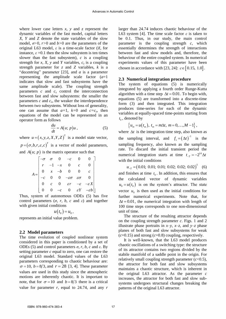
Fig. 4: Power spectral density estimates of fast (x

and z) and slow (X and Z) dynamic variables for

c=0.8.

Fig. 5: Spectrogram for fast and slow dynamic

variables for c=0.15.

1

2

0

, 0, , 1M

i M mk

k m

m

U u e k M

, (7)

where k is a discrete normalized frequency. Then

the spectrum can be represented as follows 2

, 0, , 1k

k

s

UP k M

Mf . (8)

The spectrum Pk can be plotted on a dB scale,

relative to the reference amplitude Pref =1, therefore

1010 log , 0, , 1dB

k kP P k M . (9)

The frequency fk corresponding to point k of the

DFT is

sk

ff k

M . (10)

.

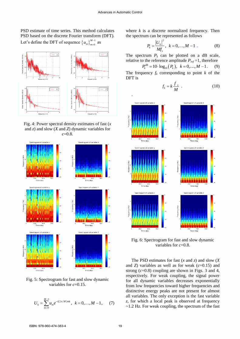
Fig. 6: Spectrogram for fast and slow dynamic

variables for c=0.8.

The PSD estimates for fast (x and z) and slow (X

and Z) variables as well as for weak (c=0.15) and

strong (c=0.8) coupling are shown in Figs. 3 and 4,

respectively. For weak coupling, the signal power

for all dynamic variables decreases exponentially

from low frequencies toward higher frequencies and

distinctive energy peaks are not present for almost

all variables. The only exception is the fast variable

z, for which a local peak is observed at frequency

~1.2 Hz. For weak coupling, the spectrum of the fast

Advances in Automatic Control

ISBN: 978-960-474-383-4 19

subsystem is similar to the spectrum of the L63

model: the fast subsystem generates a broadband

spectrum reminiscent of random noise

corresponding to irregular aperiodic oscillations. At

the same time, the low-frequency component

strongly dominates in the spectrum of slow

subsystem. As the coupling strength increases, the

power spectrum of both fast and slow subsystems

shifts toward the low frequencies, which

predominate in the spectra.

Spectrogram is another powerful technique used

in many applications for estimating the spectrum of

the time series data. Spectrogram provides

information about power as a function of frequency

and time [26], and is generally presented as plot

with the frequency of the signal shown on the

vertical axis, time on the horizontal axis, and signal

power on a colour-scale. Thus, for a given time

frame the spectrogram provides the information

about frequency content of a signal. Normalized

spectrograms for fast (x, y and z) and slow (X, Y and

Z) variables for weak (c=0.15) and strong (c=0.8)

coupling are shown in Figs. 5 and 6, respectively,

with red color representing the highest signal power

and blue the lowest. Calculated spectrograms are

fully consistent with the PSPs, providing additional

information about dominant and minor frequencies

in the spectrum for a given time.

4 Conclusion The low-order coupled chaotic dynamical system

discussed in this paper represents a powerful tool to

study various physical and computational aspects of

numerical weather prediction, data assimilation and

climate simulation. However, the NWP and climate

modeling pursue very different objectives and are

focused on dynamical processes of significantly

different spatial and time scales. The integration

time τ of the system equations can be classified

based on its duration as short, intermediate, long and

very long [27], with the corresponding values of τ

set to τ =0.1, τ =0.44, τ =2.26 and τ =131.36,

respectively. The short integration times traverse

some portion of a trajectory along the attractor, the

intermediate integrations correspond to complete

circle around the attractor, the long integrations

complete several circles, and the very long

integrations correspond to movement along the

attractor of about 100 times. The time step Δt=0.01

used in the numerical integrations is equivalent to

1.2 hours of a real time [3]. Therefore, intermediate

and long-time intervals defined above correspond to

2.2 and 11.3 days, respectively, which are consistent

with the NWP and data assimilation time of

integrations. In turn, the very long integration

intervals correspond to climate modeling time

scales.

This paper analysed the basic spectral properties

of the nonlinear chaotic coupled dynamical system

consisting of two versions of the L63 model. The

power spectral density functions and spectrograms

for dynamic variables of the fast and slow

subsystems were computed by numerical integration

of the system equations. The influence of the

coupling strength parameter on the PSDs and

spectrograms of dynamic variables was estimated.

By changing the coupling strength parameter c, one

can obtain the system behaviour that reflects the

major dynamical patterns of weather and climate for

given natural conditions

References:

[1] H.A. Dijkstra, Nonlinear climate dynamics,

Cambridge University Press, New York, 2013.

[2] W.A. Robinson, Modeling dynamical climate

systems (modeling dynamical systems),

Springer-Verlag, New York, 2001.

[3] E.N. Lorenz, Deterministic non-periodic flow,

Journal of the Atmospheric Sciences, Vol. 20,

1963, pp. 130-141.

[4] C. Sparrow, The Lorenz equations: bifur-

cations, chaos, and strange attractors,

Springer-Verlag, New York, 1982.

[5] R. Festa, A. Mazzino, and D. Vincenzi, Lorenz-

like systems and classical dynamical equations

with memory forcing: An alternate point of

view for singling out the origin of chaos,

Physical Review E, Vol. 65, Article ID 046205,

pp. 1-15.

[6] A. Pasini and V. Pelino, A unified view of

Kolmogorov and Lorenz systems, Physics

Letters A, Vol. 275, 2000, pp. 435-446.

[7] D. Roy and Z.E. Musielak, Generalized Lorenz

models and their routs to chaos. II. Energy-

conserving horizontal mode truncations, Chaos,

Solutions & Fractals, Vol. 31, 2007, pp. 747-

756.

[8] A. Trevisan and F. Pancotti, Periodic orbits,

Lyapunov vectors, and singular vectors in the

Lorenz system, Journal of the Atmospheric

Sciences, Vol. 55, 1998, pp. 390-398.

[9] M. Viana, What’s new on Lorenz strange

attractors?, The Mathematical Intelligence, Vol.

22, 2000, pp. 6-19.

[10] B. Saltzman, Finite amplitude free convection

as an initial value problem, Journal of the

Advances in Automatic Control

ISBN: 978-960-474-383-4 20

Atmospheric Sciences, Vol. 19, 1962, pp. 329-

341.

[11] T.N. Palmer, Extended-range atmospheric

prediction and the Lorenz model, Bulletin of

the American Meteorological Society, 1993,

Vol. 74, pp. 49-66.

[12] P.J. Roeber, Climate variability in a low-order

coupled atmosphere-ocean model, Tellus, Vol.

47A, 1995, pp. 473-494.

[13] J.M. Gonzalea-Miranda, Predictability in the

Lorenz low-order general atmospheric

circulation model, Physics Letters, Vol. 233,

1997, pp. 347-354.

[14] S. Sorti, F. Molteni, and T. N. Palmer, Signatu-

re of recent climate change in frequencies of

natural atmospheric circulation regimes, Letters

to Nature, Vol. 398, 1999, pp. 799-802.

[15] P. Gautier, Chaos and quadric-dimensional data

assimilation: a study based on the Lorenz

model, Tellus, Vol. 44A, 1992, pp. 2-17.

[16] G. Evensen, Inverse method and data assimi-

lation in non-linear ocean models, Physica D,

Vol. 77, 1994, pp. 108-129.

[17] R.N. Miller, M. Ghil and F. Gauthiez,

Advanced data assimilation in strongly non-

linear dynamical systems, Journal of the

Atmospheric Sciences, Vol. 59, 1994, pp. 1037-

1056.

[18] L.A. Smith, C. Ziehmann and K. Fraedrich,

Uncertainty dynamics and predictability in

chaotic systems, Quarterly Journal of the

Royal Meteorological Society, Vol. 125, 1999,

pp. 2855-2886.

[19] D.J. Lea, M.R. Allen, and T.W.N. Haine,

Sensitivity analysis of the climate of a chaotic

system, Tellus, Vol. 52A, 2000, pp. 523–532.

[20] J.A. Annan and J.C. Hargreaves, Efficient

parameter estimation for a highly chaotic

system, Tellus, Vol. 56A, 2004, pp. 520-526.

[21] G. Bofetta, A. Crisanti, F. Paparella, A.

Provenzale, and A.Vulpiani, Slow and fast

dynamics in coupled systems: A time series

analysis view, Physica D, Vol. 116, 1998, pp.

301-312.

[22] G. Bofetta, P. Giuliani, G. Paladin, and A.

Vulpiani, An extension of the Lyapunov

analysis for the predictability problem,

Journal of the Atmospheric Sciences, Vol.

55, 1998, pp. 3409-3416. [23] M. Peña and E. Kalnay, Separating fast and

slow models in coupled chaotic systems,

Nonlinear Processes in Geophysics, Vol. 11,

2004, pp. 319-327.

[24] L. Siquera and B. Kirtman, Predictability of a

low-order interactive ensemble, Nonlinear

Processes in Geophysics, Vol. 19, 2012, pp.

273-282.

[25] A.V. Oppenheimer and R.W. Schafer,

Discrete-time signal processing, Prentice Hall,

3rd edition, 2000.

[26] R.D. Hippenstiel, Detection theory: Applica-

tions and digital signal processing, CRC Press,

Boca Raton, 2002.

[27] D.J. Lea, M.R. Allen, and T.W.N. Haine,

Sensitivity analysis of the climate of a chaotic

system, Tellus, vol. 52A, 2000, pp. 523–532.

Advances in Automatic Control

ISBN: 978-960-474-383-4 21