power quality improvement using a statcom inverter · power quality improvement using a statcom...
TRANSCRIPT

University of Southern Queensland
Faculty of Health, Engineering and Sciences
Power Quality Improvement Using a STATCOM
Inverter
A dissertation submitted by
Phillip Nicholson
in fulfilment of the requirements of
ENG4111 and ENG4112 Research Project
towards the degree of
Bachelor of Engineering (Honours)
Power Engineering
Submitted: October, 2016

I
ABSTRACT
Most loads on an electrical network are reactive and have a lagging power factor,
this reactive power is mostly supplied from the electricity generators and needs to
be transmitted through the network just like any other load. The transmission of this
reactive power also increases losses and causes unnecessary heating in
infrastructure.
An increase in Photovoltaic (PV) penetration in an electrical system has imposed
several Power Quality (PQ) and voltage stability issues, the intermittent nature of
solar generation mean there is a variable output of power to the system which leads
to power imbalance issues and voltage sags and swells. A solution to this may in
fact lie in the problem, there is a potential for the installed inverters associated with
these systems to be utilised to improve local power quality by supplying or
absorbing reactive power, day or night. Currently inverters are only being utilised
during daylight hours, leaving an expensive piece of equipment lying dormant for
the majority of a day.
This research outlines the gathering of relevant information, compiles a feasibility
assessment and documents expected outcomes and benefits. A research
methodology is provided together with a risk assessment, project schedule and
quality assurance plan and timeline.
This research will provide useful information into the feasibility of grid controlled
Static Compensator (STATCOM) inverters and the benefits this would have on
power factor and subsequently voltage regulation to the immediate network.

II
University of Southern Queensland
Faculty of Health, Engineering and Sciences
ENG4111 and ENG4112 Research Project
Limitations of Use
The Council of the University of Southern Queensland, its Faculty of Health,
Engineering and Sciences, and the staff of the University of Southern Queensland,
do not accept any responsibility for the truth, accuracy or completeness of material
contained within or associated with this dissertation.
Persons using all or any part of this material do so at their own risk, and not at the
risk of the Council of the University of Southern Queensland, its Faculty of Health,
Engineering and Sciences or the staff of the University of Southern Queensland.
This dissertation reports an educational exercise and has no purpose or validity
beyond this exercise. The sole purpose of the course pair entitles “Research Project”
is to contribute to the overall education within the student’s chosen degree program.
This document, the associated hardware, software, drawings, and any other material
set out in the associated appendices should not be used for any other purpose: if
they are so used, it is entirely at the risk of the user.

III
CERTIFICATION
I certify that the ideas, designs and experimental work, results, analyses and
conclusions set out in this dissertation are entirely my own effort, except where
otherwise indicated and acknowledged.
I further certify that the work is original and has not been previously submitted for
assessment in any other course or institution, except where specifically stated.
Name: Phillip Nicholson
Student Number: 61040542
Date: 4th October, 2016
__________________________________
Signature

IV
ACKNOWLEDGEMENT
This research project would not have been possible without the assistance of Dr Les
Bowtell. The topic was chosen with guidance from Les after discussions
surrounding my interest in renewable energy and a more efficient future. Les’
involvement in the project included assisting in the research and dissecting results
from the field survey. He suggested areas that required further investigation and
improvements to my site surveying technique. I thank Les sincerely for his
encouraging guidance, friendly advice and generous time donated to me throughout
this project.
I would also like to thank my family, especially my wife and daughter, thank you
for encouraging me in all of my pursuits and inspiring me to complete this degree.
I always knew that you believed in me, you have been my inspiration I needed
during the years of study.

V
TABLE OF CONTENTS
Contents Page
ABSTRACT ............................................................................................................ I
CERTIFICATION .............................................................................................. III
ACKNOWLEDGEMENT .................................................................................. IV
TABLE OF CONTENTS ..................................................................................... V
LIST OF FIGURES ............................................................................................ IX
LIST OF TABLES .............................................................................................. XI
NOMENCLATURE ........................................................................................... XII
CHAPTER 1 ........................................................................................................... 1
INTRODUCTION ................................................................................................. 1
1.1 Outline of the Study ................................................................................. 1
1.2 Background .............................................................................................. 1
1.2.1 Solar Energy ........................................................................................ 1
1.2.2 STATCOM .......................................................................................... 2
1.2.3 The Problem ......................................................................................... 2
1.3 Project Aim .............................................................................................. 3
1.4 Project Objective ...................................................................................... 3
1.5 Thesis Overview ...................................................................................... 3
1.6 Summary .................................................................................................. 4
CHAPTER 2 ........................................................................................................... 5
LITERATURE REVIEW ..................................................................................... 5
VI
2.1 Overview .................................................................................................. 5
2.2 Reactive Powers Effect on Voltage Regulation ....................................... 5
2.3 Reactive Power Control in a Distribution Network ................................. 6
2.3.1 Generators ............................................................................................ 6
2.3.2 Reactors and Capacitor Banks ............................................................. 6
2.3.3 Static Compensator (STATCOM) ....................................................... 7
2.4 Control of STATCOM’s Reactive Power Output .................................... 7
2.5 Power Quality .......................................................................................... 8
2.6 Smart Meters ............................................................................................ 9
2.7 Grid connected PV systems with battery storage .................................. 10
2.7.1 PV Impacts on PQ .............................................................................. 11
2.7.2 Intermittency of PV Systems ............................................................. 12
2.8 ITI (CBEMA) Curve .............................................................................. 13
2.9 Voltage Control ...................................................................................... 14
2.10 Review of Information ........................................................................... 14
CHAPTER 3 ......................................................................................................... 15
RESEARCH AND TEST METHODOLOGY .................................................. 15
3.1 PQ Survey Sites ..................................................................................... 15
3.2 Contingency Plan for PQ Survey ........................................................... 16
3.3 PQ Survey .............................................................................................. 16
3.3.1 PQ Meter ............................................................................................ 16
3.3.2 Meter Installation / Recovery Procedure ........................................... 17
3.3.3 Meter Configuration Settings ............................................................. 18
3.3.4 Event Trigger Settings ....................................................................... 19
3.4 Bureau of Meteorology Information ...................................................... 20
3.5 Development of the System Model ....................................................... 20
VII
3.5.1 Industrial System Model Calculations ............................................... 23
3.5.2 Commercial System Model Calculations .......................................... 24
3.5.3 Residential Rural System Model ....................................................... 25
3.6 Power Flow Analysis in MATLAB ....................................................... 26
3.7 Risk Assessment .................................................................................... 28
3.7.1 PQ Survey Risks ................................................................................ 29
3.7.2 PQ Survey Data Risks ........................................................................ 29
3.7.3 MATLAB Simulation Risks .............................................................. 30
CHAPTER 4 ......................................................................................................... 31
DATA AND RESULTS ANALYSIS .................................................................. 31
4.1 STATCOM on a Single Bus During Normal Conditions ...................... 31
4.1.1 Industrial Modelled Systems during Peak Load ................................ 32
4.1.2 Industrial Modelled Systems during Off-Peak Load ......................... 34
4.1.3 Commercial Modelled Systems Peak Load ....................................... 36
4.1.4 Commercial Modelled Systems Off-Peak Load ................................ 38
4.1.5 Residential Modelled Systems during Peak Load ............................. 40
4.1.6 Residential Modelled Systems during Off-Peak Load ...................... 42
4.2 STATCOM on a Single Bus During Transient Conditions ................... 44
CHAPTER 5 ......................................................................................................... 48
DISCUSSION AND IMPLICATIONS .............................................................. 48
5.1 STATCOM used for Power Factor Improvement ................................. 48
5.1.1 Power Factor During Transients ........................................................ 49
5.2 STATCOM used for Full Voltage Regulation ....................................... 49
5.2.1 Voltage Regulation During Transients .............................................. 50
5.3 Compliance with Current Australian Standards .................................... 51
5.4 Multiple STATCOM Installations ......................................................... 51
VIII
5.5 STATCOM Active and Reactive Power Supply ................................... 51
CHAPTER 6 ......................................................................................................... 53
CONCLUSIONS .................................................................................................. 53
6.1 PQ Improvements using a STATCOM Inverter .................................... 53
6.2 Future Research ..................................................................................... 54
6.2.1 Investigate feeder with High PV Penetration and VR Issues ............ 54
6.2.2 Communication between SMART Meter and SMART Grid ............ 55
6.2.3 Review of Current Standards for Inverters ........................................ 55
REFERENCES ..................................................................................................... 56
APPENDICES ...................................................................................................... 60
Appendix A - Project Specification ................................................................... 60
Appendix B - Project Risk Assessment ............................................................. 62
Appendix C - Project Timeline .......................................................................... 65
Appendix D - Resource Requirements ............................................................... 69
Appendix E - MATLAB Programs .................................................................... 72
Appendix F - Hazard Assessment Check Forms ................................................ 80
Appendix G - PQ Survey Data ........................................................................... 84
Appendix H - Literature Review ........................................................................ 88

IX
LIST OF FIGURES
Figure 2.1 Principle Operation of a STATCOM (Yohan Fajar Sidik, 2012) .......... 8
Figure 2.2 Grid-Tied PV System with Battery Storage (Solar 2016) .................... 11
Figure 2.3 Typical PV System Generation (University 2016) ............................... 12
Figure 2.4 ITI Curve ((ITI) 2000) .......................................................................... 13
Figure 3.1 PQ-Box 100 network analyser used to survey selected sites .............. 17
Figure 3.2 PQ Meter installed at Manly on transformer cabling .......................... 18
Figure 3.3 PQ Meter Setup for Basic Settings ...................................................... 19
Figure 3.4 PQ Meter Event Trigger Settings ........................................................ 20
Figure 3.5 Radial System Model Used for all Load Profiles ................................. 21
Figure 3.6 Dynamic Load Profiles for SDG&E (Anders 2015) ............................ 22
Figure 4.1 Industrial Models Bus Voltages during Peak Load .............................. 33
Figure 4.2 Industrial Models Power Factor during Peak Load .............................. 34
Figure 4.3 Industrial Models Bus Voltages during Off-Peak Load ....................... 35
Figure 4.4 Industrial Models Power Factor during Off-Peak Load ....................... 36
Figure 4.5 Commercial Models Bus Voltages during Peak Load ......................... 37
Figure 4.6 Commercial Models Power Factor during Peak Load ......................... 38
Figure 4.7 Commercial Models Bus Voltages during Off-Peak Load .................. 39
Figure 4.8 Commercial Models Power Factor during Off-Peak Load .................. 40
Figure 4.9 Residential Models Bus Voltages during Peak Load ........................... 41
Figure 4.10 Residential Models Power Factor during Peak Load ......................... 42
X
Figure 4.11 Residential Models Bus Voltages during Off-Peak Load .................. 43
Figure 4.12 Residential Models Power Factor during Off-Peak Load .................. 44
Figure 4.13 Industrial Model Bus Voltage during Transient Condition ................ 46
Figure 4.14 Industrial Model Power Factor during Transient Condition .............. 47
Figure 5.1 STATCOM Size Required for Full Voltage Regulation at Bus 4 ........ 50
Figure G-1 Real Power Consumption at Atarmon Site ......................................... 84
Figure G-2 Reactive Power Consumption at Artarmon Site ................................. 85
Figure G-3 Real Power Consumption for Manly High-rise .................................. 86
Figure G-4 Reactive Power Consumption for Manly High-rise ............................ 87

XI
LIST OF TABLES
Table 3.1 TX and Line Data for Industrial System Model .................................... 24
Table 3.2 TX and Line Data for Commercial System Model ................................ 24
Table 3.3 TX and Line Data for Rural System Model ........................................... 25
Table 4.1 Industrial Model Bus and Load Data during Peak Load ....................... 33
Table 4.2 Industrial Model Bus and Load Data during Off-Peak Load ................ 35
Table 4.3 Commercial Model Bus and Load Data during Peak Load ................... 37
Table 4.4 Commercial Model Bus and Load Data during Off-Peak Load ............ 39
Table 4.5 Residential Model Bus and Load Data during Peak Load ..................... 41
Table 4.6 Residential Model Bus and Load Data during Off-Peak Load .............. 43
Table 4.7 Industrial Model Bus and Load Data during Transient Conditions ....... 46
Table B-1 Personal Risk Matrix - Be Safe Pro 10 Managing WHS ...................... 62
Table B-2 Personal Risk Assessment .................................................................... 63
Table B-3 Project Risk Assessment ....................................................................... 64
Table C-1 Project Timeline .................................................................................... 66
Table C-2 Project Timeline .................................................................................... 67
Table C-3 Project Timeline ................................................................................... 68
Table D-1 Project Resources ................................................................................ 69
Table D-2 Project Resources ................................................................................ 70
Table D-3 Project Resources ................................................................................ 71
XII
NOMENCLATURE
The following abbreviations have been used throughout the text: -
PV
DC
AC
CT
STATCOM
FACTS
PQ
PLCC
PLN
THD
VSI
Hz
VAr
VSC
TX
LV
HV
USQ
Photovoltaic
Direct Current
Alternating Current
Current Transformer
Static Compensator
Flexible Alternating Current Transmission System
Power Quality
Power Line Communication
Power Line Networking
Total Harmonic Distortion
Voltage Source Inverter
Hertz
Reactive Power
Voltage Source Converter
Transformer
Low Voltage
High Voltage
University of Southern Queensland

1
INTRODUCTION
1.1 Outline of the Study
There is a need to become more efficient with our energy usage, this includes not
only reducing energy demand, but improving the way in which energy is being
delivered. This study is an ongoing look at the feasibility of converting existing
solar system inverters to STATCOMs. Under the proposal the local energy
requirements would not only be supplied by a customer’s solar system, but could
also help improve the PQ of surrounding electrical installations.
The broader study will investigate the impact of converting an installed inverter, or
replacing a near end of life inverter with a STATCOM, and what benefits that will
have to not only the local installation, but also upstream and downstream customers
as well as the electricity distributor. A STATCOM is a voltage source converter
made up of power electronics, it is currently used on large installations for power
factor correction, and on electricity grids for voltage regulation (VR). A
STATCOM has the added benefit of being able to rapidly respond to changes in PQ
and rectify them within their rated capacity.
1.2 Background
1.2.1 Solar Energy
The potential for future shortages of fossil-fuel sources of electric power has led to
the development of the technology needed to use non-polluting renewable fuel
sources such as the sun, wind, and fuel cells (Kirawanich & O'Connell 2000).
Generation of solar energy using small scale PV arrays is becoming increasingly
common amongst residential electrical consumers as a means of offsetting their
carbon footprint. These PV modules convert the sunlight into a Direct Current (DC)

2
voltage; this can then be converted into an Alternating Current (AC) voltage via the
means of an inverter so it can be used in parallel with the electricity grid.
1.2.2 STATCOM
A STATCOM invertor is a Flexible Alternating Current Transmission System
(FACTS), it is used to control the power flow through an electrical transmission
line (Sen 1999). By absorbing and supplying reactive power the STATCOM can
control the power factor of a local load by altering the phase angle of the current in
relation to the voltage. The STATCOM can either be connected directly to the
generation source or can be used through a storage device such as a battery. Many
of these devices are active during the day but often lay dormant during the night
time when there is no sunlight. The ideal output of a STATCOM would be a pure
sinusoidal AC waveform, but this is not possible even with the most advanced
technology, there still exists a small DC output from the inverter into the grid. There
are limits the electricity distribution authority will allow of this DC output and also
the amount of harmonic distortion.
1.2.3 The Problem
There is potential for STATCOM inverters used in Solar PV arrays to improve PQ
at the local premises as well as the local electrical grid. This could be done around
the clock as opposed to the relatively short hours of operation that the inverters are
used now during daylight hours only. As the many of the initial batch of inverters
purchased in Australia circa 2007. Purchased under the federal government PV
rebate scheme, reach their expected life cycles in the next few years, it is a poignant
time to look for smarter alternatives for the estimated 10-20yrs of the installed PV
panels.
The electricity grid’s voltage is dependent on the amount of reactive power that is
needed and hence can be controlled with the inducement or absorption of reactive
power. This can be done remotely or preferable locally, as locally will not require
the transmission of the reactive power over long distances.

3
1.3 Project Aim
The aim of this work is to carry out power surveys on a selection of sites that have
a PV array installed. The load survey will include load cycle information as well as
apparent and reactive power readings. Records from the Australian Bureau of
Meteorology on the radiance of the sites will also be used. This will provide the
radiance during the time of the survey at each site, the use of this data will avoid
the need to survey the radiance at the same time as the power survey.
The results from the survey will then be modelled in MATLAB so they can be
simulated with a known accurate simulation of a STATCOM inverter, previously
created by Dr Les Bowtell.
1.4 Project Objective
The specific objectives of this project area: -
1. Conduct a literature review on the STATCOM inverter and their PQ
improvement capabilities. Using the literature review determine if these
capabilities are going to be able to provide a significant improvement to the
PQ at selected premises.
2. Perform a load survey of a commercial and high density residential load.
3. Analyse load data and develop a system model for use in MATLAB.
4. Evaluate the transient capabilities of a STATCOM inverter on the system
loads modelled in MATLAB.
5. Report on the potential benefits that can be expected to both the consumer
and electricity distributor from a locally installed STATCOM.
1.5 Thesis Overview
Chapter 2 of the dissertation contains the literature review which has been carried
out to better understand the research subject. Previous techniques for controlling
PQ by the electricity distributors and locally are explored and weighed up.

4
Chapter 3 outlines the methodology that was adopted for completing this project,
whilst Chapter 4 reports the data obtained from the load surveys and the results
from the simulation of the system loads modelled in MATLAB. Chapter 5 contains
the in depth discussion surrounding the results.
Finally, Chapter 6 will provide recommendations and conclusions on the study, as
well as suggestions for future research into the development of this project.
1.6 Summary
As can clearly be seen this project will test the feasibility of converting existing
solar system inverters into STATCOMs for the purpose of supplying reactive power
to improve PQ. There is a clear and present need for this study as we shift more of
our load onto renewable energies and look to becoming more energy efficient. It is
hoped this research will offer an alternative method to solving PQ issues on the
network using existing equipment.

5
LITERATURE REVIEW
2.1 Overview
A literature review was undertaken to further develop the idea towards a research
project. The purpose of the review was to gather relevant information about:
Reactive power effect on voltage regulation
Control of STATCOM’s reactive power
Power Quality
SMART meters
Grid connected PV systems with battery storage
ITI Curve
The literature review is provided as Appendix A, the following is a brief summary
of the more important points. The review is expected to be continuously revised
throughout the length of the project.
2.2 Reactive Powers Effect on Voltage Regulation
A study by Petoussis (Petoussis et al. 2006) has found that the presence of reactive
power in the network has a significant impact on the electricity market equilibrium
and the power distribution in the network. Reactive power and voltage control is
one of the ancillary services used to maintain the voltage profile through injecting
or absorbing reactive power (Dapu et al. 2005).
If the voltage on a system is too low it will not be able to supply active power, thus
reactive power is required to provide the voltage levels needed on the system. An
increase in reactive power being supplied by the electricity distributor means more
power is required to be transmitted down the suppliers’ infrastructure which will

6
increase losses. During times of high load there is a drop in voltage in the network,
as the voltage drops there is an increase in current to maintain the amount of power
supplied. This causes the system to absorb more reactive power and thus the voltage
drops even further potentially creating a cascading effect until voltage failure.
2.3 Reactive Power Control in a Distribution Network
There are a number of ways reactive power can be controlled in a distribution
network, some with static control equipment and some dynamic. Examples of the
more common control will be discussed in this review.
2.3.1 Generators
An electric generators main function is to convert energy into electric power, this
output power can be considered in terms of their terminal voltage and their reactive
power output. Reactive power is produced by increasing the magnetic field in the
generator by increasing the current in the rotating field winding. Production of
reactive power limits a generators real-power production and so ideally it would be
desirable to be kept to a minimum.
2.3.2 Reactors and Capacitor Banks
Electricity distributors install reactors and capacitor banks at the local zone
substations to assist with the generation and absorption of reactive power for the
local area. A capacitor bank will produce reactive power at times of high load where
the voltage in the system has dropped. A reactor will absorb reactive power when
the network voltage is high, normally during low load periods such as the late
evening to early morning. They are both passive devices and as such need to be
switched on and off, usually after the network voltage has reached a set limit away
from nominal.

7
2.3.3 Static Compensator (STATCOM)
A Static Compensator (STATCOM) is a device that can provide reactive support to
a bus. It consists of a voltage sourced converters connected to an energy storage
device on one side and to the power system on the other (Rao, Crow & Yang 2000).
It is a power electronics device, consisting of insulated-gate bipolar transistor’s
(IGBT) which have a high efficiency and fast switching. Currently they are used on
the electricity grid by the distributor, or as part of large commercial installations for
power factor correction.
2.4 Control of STATCOM’s Reactive Power Output
Studies from Escobar (Escobar, Stankovic & Mattavelli 2000) has found that
STATCOM’s offer several advantages over conventional thyristor-based
convertors solutions for voltage control due to that speed of response, flicker
compensation, flexibility, and minimal interaction with the supply grid.
The output of the STATCOM’s power can be controlled by adjusting the phase
angle between the voltage and current, this is shown in Figure 2.1. If a leading phase
angle is needed then reactive power will be absorbed by the STATCOM by,
however if a lagging phase angle is applied then the STATCOM will produce
reactive power. This control of the STATCOM can be carried out by using a VAr
controller. This VAr controller can be installed locally to the STATCOM to assist
with improving the power factor of the local load by supplying or absorbing reactive
power as needed. The VAr controller can be implemented with the use of logic
algorithms and a programmable logic controller (PLC).

8
Figure 2.1 Principle Operation of a STATCOM (Yohan Fajar Sidik, 2012)
2.5 Power Quality
The term PQ has been used to describe the variation of the voltage, current, and
frequency on the power system (Reid 1994). Maintaining PQ on an electrical
system refers to maintaining a near perfect sinusoidal waveform of voltage and
current. Many factors on an electrical system can alter and distort these waveforms
including, harmonics, unbalanced loads, transformer vibration and noise. Harmonic
distortion of the power waveform occurs when the fundamental, second, third and
other harmonics are combined. The result is voltage and current contaminations on
the sinusoidal waveform (Henderson & Rose 1993). Poor PQ on a system can lead
to problems with overvoltage, voltage unbalance, dips and swells, and harmonics.

9
2.6 Smart Meters
SMART meters will play a very important role in the future with customers having
an increased interest in how much energy they used and when. The old disc meters
were only able to give limited energy usage information such as how much was
used, and an indication of how much was being used currently was only possible
by seeing how fast the disc was spinning. The advent of the SMART meter allows
energy companies to charge in a tariff known as time of use, where energy can be
charged at different amounts depending on what time of the day it is being
consumed.
The increase in embedded generation has also seen an increase in SMART meters
as these meters are required for such generation as they allow for a bidirectional
energy flow between the grid and the consumer.
Communication with the SMART meter can be done in a variety of ways, the three
most common ways that have been reviewed by Ali (Ali, Maroof & Hanif 2010)
are:
RS-232 As Local transmission medium
PLCC Using main power line
Short Messaging Service on GSM
Power line communication (PLCC) or Power line networking (PLN) which utilises
the same wired medium through which power is delivered to the customer as a
communication channel (Ali, Maroof & Hanif 2010). This is the medium that will
be focused on in this project as no further wiring would be required.

10
2.7 Grid connected PV systems with battery storage
Junbiao (Junbiao et al. 2012) states that the integration of PV generation brings
numerous challenges to the system operators and designers such as:
Changing solar irradiance profile.
Remote location of PV due to solar energy.
Inability to meet expected energy output levels without storage or auxiliary
device.
Active power can be balanced by STATCOM with battery storage when battery is
charged when system voltage is higher than upper set value, and discharged when
system voltage is lower than lower set value (Junbiao et al. 2012).
It is expected that as the manufacturing costs of battery storage comes down there
will be an increased uptake of this energy storage at the consumer level. With the
increase of battery storage there is real potential for power factor correction to be
carried out locally rather that via large reactors and capacitor banks that are
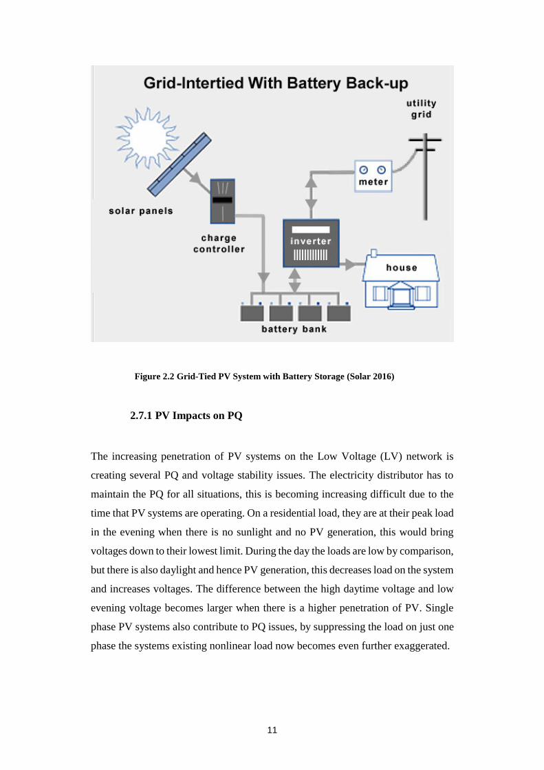
currently operated and maintained by the electricity distributors. Figure 2.2
represents a typical grid-tied PV system on a household with battery storage. The
sun’s energy is converted into DC which is either stored in the battery or converted
into AC via the inverter to be used around the house or supplied back into the grid.
11
Figure 2.2 Grid-Tied PV System with Battery Storage (Solar 2016)
2.7.1 PV Impacts on PQ
The increasing penetration of PV systems on the Low Voltage (LV) network is
creating several PQ and voltage stability issues. The electricity distributor has to
maintain the PQ for all situations, this is becoming increasing difficult due to the
time that PV systems are operating. On a residential load, they are at their peak load
in the evening when there is no sunlight and no PV generation, this would bring
voltages down to their lowest limit. During the day the loads are low by comparison,
but there is also daylight and hence PV generation, this decreases load on the system
and increases voltages. The difference between the high daytime voltage and low
evening voltage becomes larger when there is a higher penetration of PV. Single
phase PV systems also contribute to PQ issues, by suppressing the load on just one
phase the systems existing nonlinear load now becomes even further exaggerated.
12
2.7.2 Intermittency of PV Systems
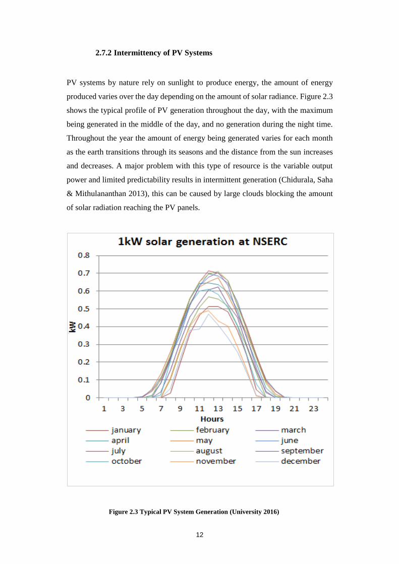
PV systems by nature rely on sunlight to produce energy, the amount of energy
produced varies over the day depending on the amount of solar radiance. Figure 2.3
shows the typical profile of PV generation throughout the day, with the maximum
being generated in the middle of the day, and no generation during the night time.
Throughout the year the amount of energy being generated varies for each month
as the earth transitions through its seasons and the distance from the sun increases
and decreases. A major problem with this type of resource is the variable output
power and limited predictability results in intermittent generation (Chidurala, Saha
& Mithulananthan 2013), this can be caused by large clouds blocking the amount
of solar radiation reaching the PV panels.
Figure 2.3 Typical PV System Generation (University 2016)
13
2.8 ITI (CBEMA) Curve
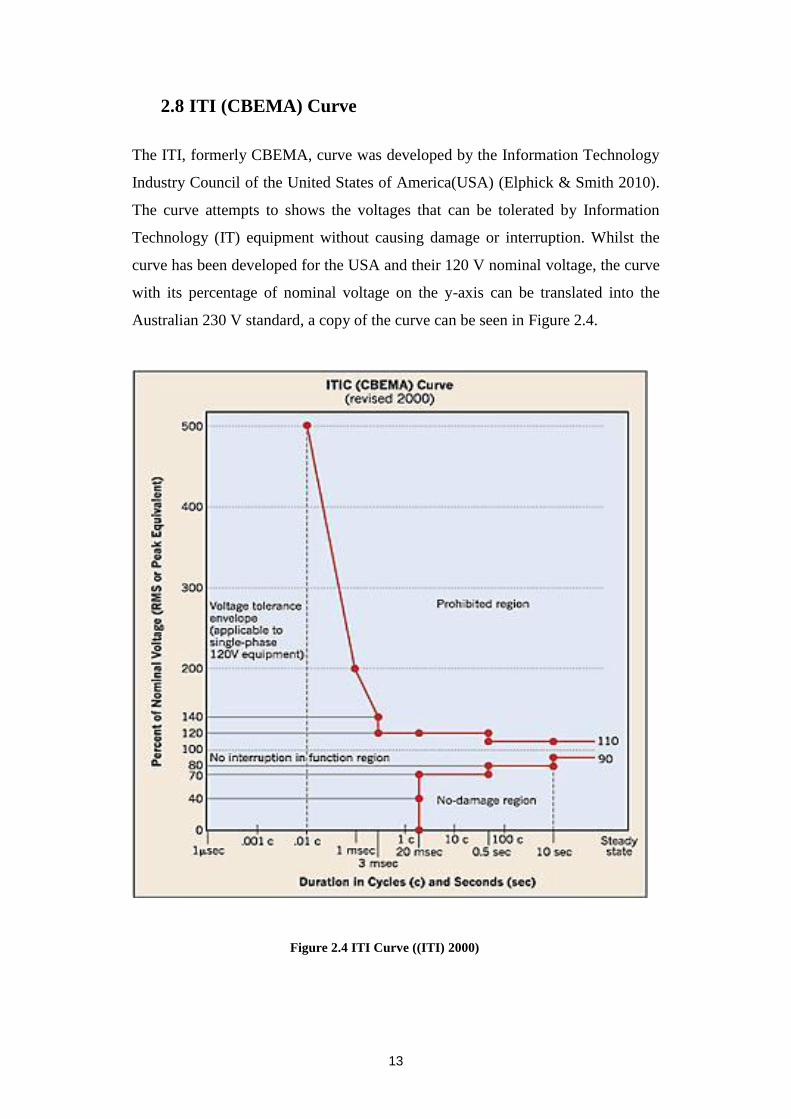
The ITI, formerly CBEMA, curve was developed by the Information Technology
Industry Council of the United States of America(USA) (Elphick & Smith 2010).
The curve attempts to shows the voltages that can be tolerated by Information
Technology (IT) equipment without causing damage or interruption. Whilst the
curve has been developed for the USA and their 120 V nominal voltage, the curve
with its percentage of nominal voltage on the y-axis can be translated into the
Australian 230 V standard, a copy of the curve can be seen in Figure 2.4.
Figure 2.4 ITI Curve ((ITI) 2000)

14
The x-axis represents the time spent in that range. There are two prohibited regions
on the curve, the upper region is for over voltages and will likely cause damage to
IT equipment. The lower region is for under voltages and whilst it is unlikely it will
cause damage to electronic equipment it will tend to cause interruptions.
2.9 Voltage Control
On an AC system voltage control is managed by absorbing and producing reactive
power. Managing reactive power in this way in affect changes the phase shift
between the current and the supply voltage, producing reactive power will have a
capacitive effect and will cause a leading power factor, whereas absorbing reactive
power will have an inductive effect and cause a lagging power factor. Tanaka
(Tanaka et al. 2009) states that reactive power control has a possibility to contribute
for reduction of distribution loss. In 2011 the Australian Standards PQ Committee
published AS 61000.3.100-2011 (Standards 2011), this defines that the voltage at a
premises needs to be within the rage of 230 V +10% or -6%. The further away from
a transformer (TX) a supply is generally means the lower their supply voltage will
be. This problem is worsened during periods of high load, which for residential
loads tends to be in the early evening.
2.10 Review of Information
It is clear from the literature review that using a STATCOM inverter to improve
power factor is efficient and has a fast response, which will be ideal in the scope of
this project as the power factor will be read in real time from the SMART meter.
The STATCOM will act as either capacitor or inductor as it is instructed to absorb
or produce reactive power when improving power factor. Communication with the
SMART meter will be carried out using Power Line Communication which will
negate the need for extra wiring.
Further review will be required throughout the project to improve knowledge in
these areas and any further areas uncovered or recommended by the supervisor.

15
RESEARCH AND TEST METHODOLOGY
3.1 PQ Survey Sites
PQ surveys were collected from various sites around the Northern Sydney region
during the Autumn and Winter months in 2016. Targeted sites for the survey were
either a medium density apartment block or a mix commercial and residential
property needing to have a solar PV array installed. A variety of sites were initially
chosen and PV arrays confirmed using the high resolution aerial imagery service
from nearmaps. Only two sites, one of each load profile was required so the list was
narrowed down to sites with a supply from above ground substations to facilitate
an easier and safer installation of the PQ meter. The measurement device was
installed and left capturing for the same length of time. Sites chosen for the survey
were:
High-rise Building in Manly – Mixed residential and commercial load
Apartment Block in Artarmon – Residential load
Unfortunately, time did not permit the survey of an industrial factory and previous
surveys carried out were not set at a suitable time interval for this projects
requirements. At each of the above sites their load was surveyed over a period of
one week. Although due to the finite amount of internal memory in the PQ meter a
whole week was sometimes not possible to be captured depending on how many
events were captured. The PQ meter was installed at the supplying substation of the
load. Ideally the meters would have been best installed on the terminals of the
customer’s main switchboard, but access to these terminals was not possible due to
security metering tags clipped onto the protective covers preventing unauthorized
access or meter tampering.

16
3.2 Contingency Plan for PQ Survey
If the required measurement devices are not available for use on my project, or the
data I obtain from the survey is corrupt or unusable, a contingency plan was devised.
Numerous surveys are carried out as part of the distributor’s Low Voltage Network
PQ Survey every year to ensure that suitable conditions provided to customers in
terms of voltage ranges, voltage fluctuations, and voltage harmonics etc. are being
adhered to. It was decided that in the event a survey specifically carried out for this
project was unable to occur, two surveys previously carried out on suitable sites
would be obtained from the distributor with permission and used as part of this
research project.
3.3 PQ Survey
All survey work was carried out around Northern Sydney during the second quarter
of 2016. Measuring equipment and software to download the data was provided by
the company, as was the person protective equipment used when installing and
recovering the metering equipment. Risk assessments were carried out for the
hazardous work and copies can be found in Appendix B -. Pre work hazard
assessment checks were also carried out before any works, these can be found in
Appendix F -.
3.3.1 PQ Meter
In this survey the sites were each monitored for one week by a high end PQ meter
for a range of PQ parameters including Current, Voltage, Energy (P, Q, P+, P-, Q+,
Q-), Harmonics & Total Harmonic Distortion (THD), Voltage Fluctuations
(Flicker) and Frequency. The measurement device used for the survey was a PQ-
Box 100 Network Analyser, shown in Figure 3.1. This meter is suitable for low,
medium and high-voltage networks. The meter has annual calibration and was
within calibration for the entire surveying timeline.
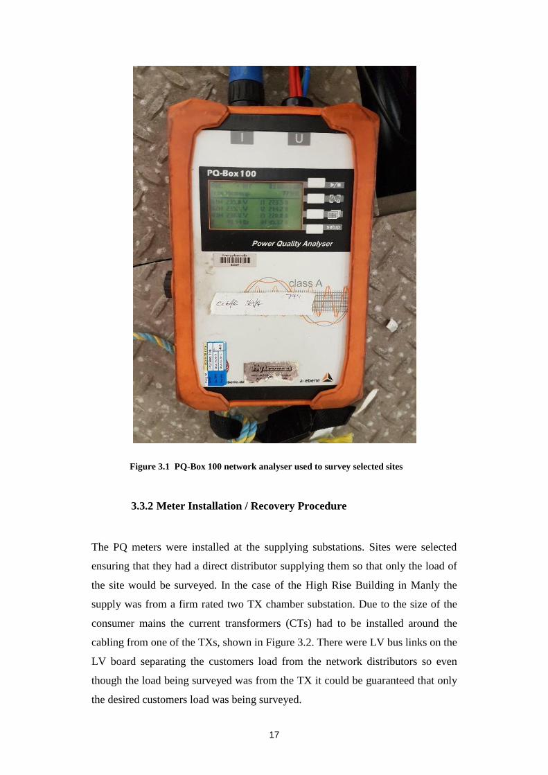
17
Figure 3.1 PQ-Box 100 network analyser used to survey selected sites
3.3.2 Meter Installation / Recovery Procedure
The PQ meters were installed at the supplying substations. Sites were selected
ensuring that they had a direct distributor supplying them so that only the load of
the site would be surveyed. In the case of the High Rise Building in Manly the
supply was from a firm rated two TX chamber substation. Due to the size of the
consumer mains the current transformers (CTs) had to be installed around the
cabling from one of the TXs, shown in Figure 3.2. There were LV bus links on the
LV board separating the customers load from the network distributors so even
though the load being surveyed was from the TX it could be guaranteed that only
the desired customers load was being surveyed.
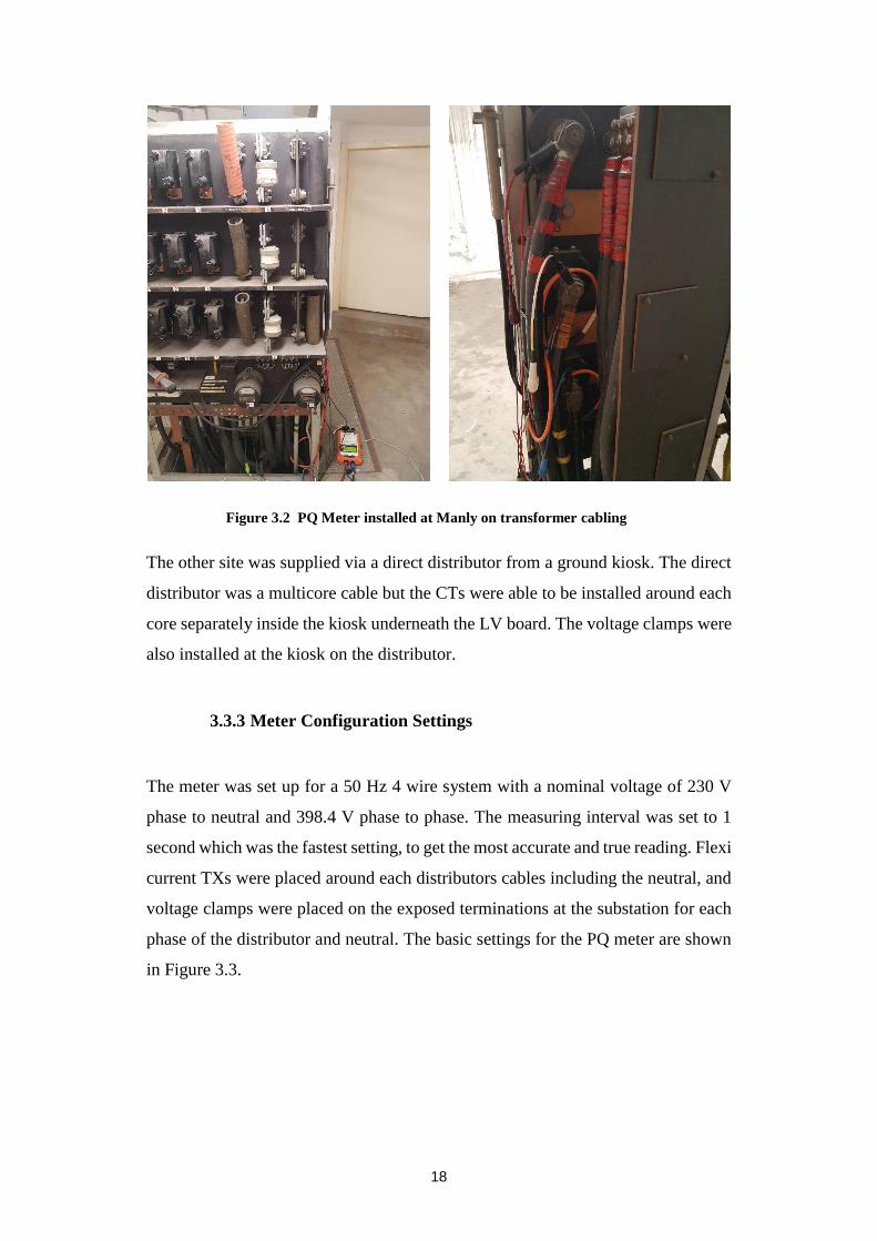
18
Figure 3.2 PQ Meter installed at Manly on transformer cabling
The other site was supplied via a direct distributor from a ground kiosk. The direct
distributor was a multicore cable but the CTs were able to be installed around each
core separately inside the kiosk underneath the LV board. The voltage clamps were
also installed at the kiosk on the distributor.
3.3.3 Meter Configuration Settings
The meter was set up for a 50 Hz 4 wire system with a nominal voltage of 230 V
phase to neutral and 398.4 V phase to phase. The measuring interval was set to 1
second which was the fastest setting, to get the most accurate and true reading. Flexi
current TXs were placed around each distributors cables including the neutral, and
voltage clamps were placed on the exposed terminations at the substation for each
phase of the distributor and neutral. The basic settings for the PQ meter are shown
in Figure 3.3.
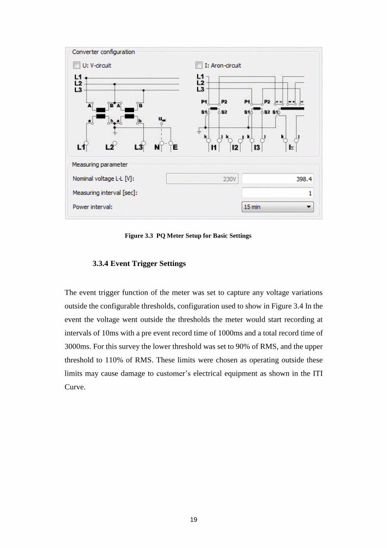
19
Figure 3.3 PQ Meter Setup for Basic Settings
3.3.4 Event Trigger Settings
The event trigger function of the meter was set to capture any voltage variations
outside the configurable thresholds, configuration used to show in Figure 3.4 In the
event the voltage went outside the thresholds the meter would start recording at
intervals of 10ms with a pre event record time of 1000ms and a total record time of
3000ms. For this survey the lower threshold was set to 90% of RMS, and the upper
threshold to 110% of RMS. These limits were chosen as operating outside these
limits may cause damage to customer’s electrical equipment as shown in the ITI
Curve.
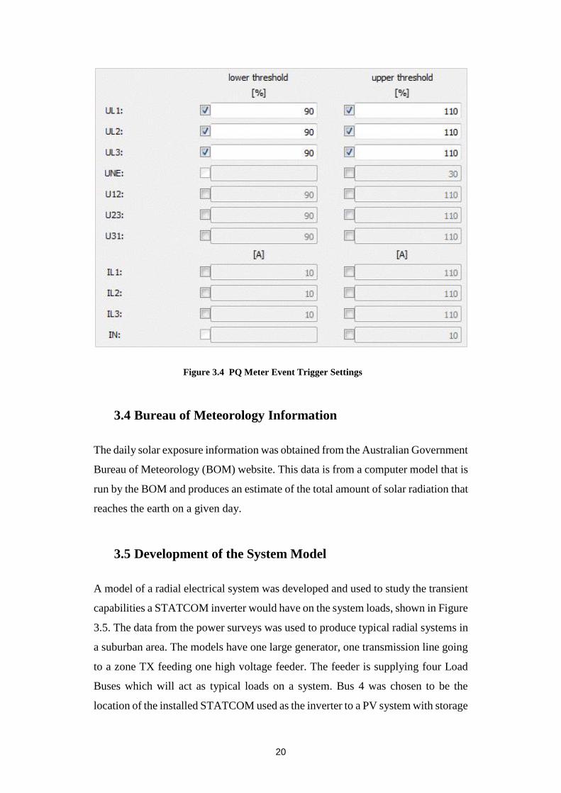
20
Figure 3.4 PQ Meter Event Trigger Settings
3.4 Bureau of Meteorology Information
The daily solar exposure information was obtained from the Australian Government
Bureau of Meteorology (BOM) website. This data is from a computer model that is
run by the BOM and produces an estimate of the total amount of solar radiation that
reaches the earth on a given day.
3.5 Development of the System Model
A model of a radial electrical system was developed and used to study the transient
capabilities a STATCOM inverter would have on the system loads, shown in Figure
3.5. The data from the power surveys was used to produce typical radial systems in
a suburban area. The models have one large generator, one transmission line going
to a zone TX feeding one high voltage feeder. The feeder is supplying four Load
Buses which will act as typical loads on a system. Bus 4 was chosen to be the
location of the installed STATCOM used as the inverter to a PV system with storage
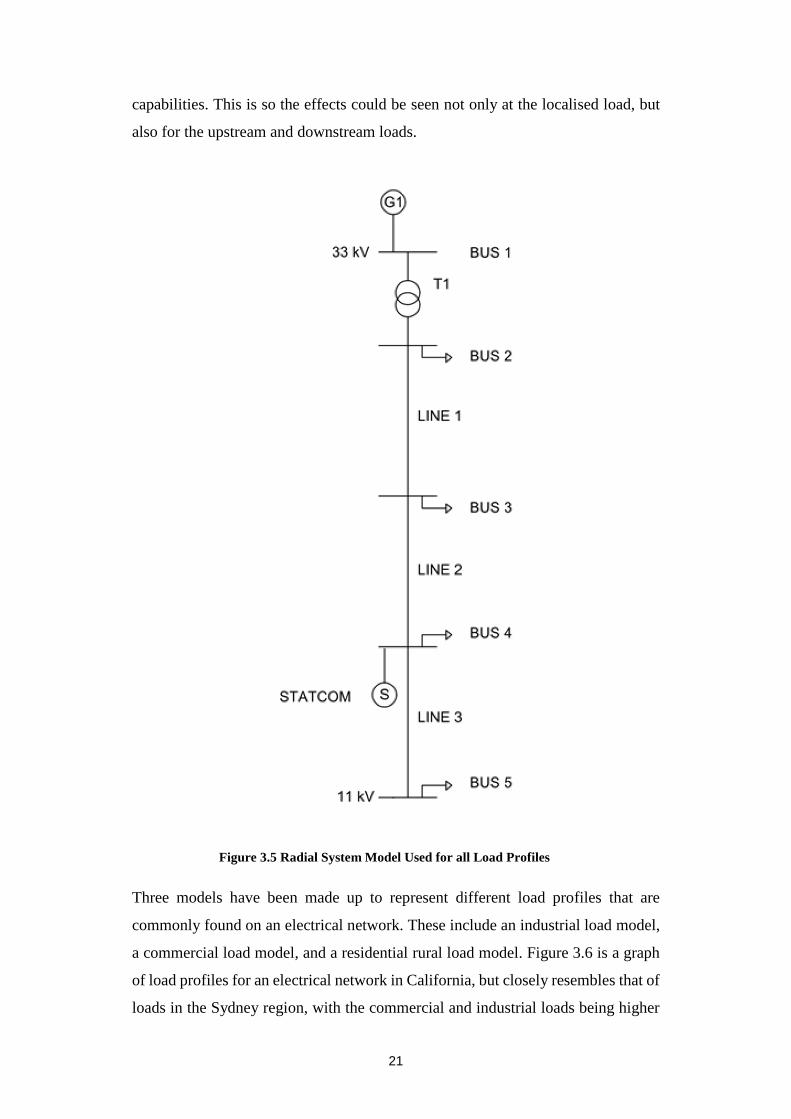
21
capabilities. This is so the effects could be seen not only at the localised load, but
also for the upstream and downstream loads.
Figure 3.5 Radial System Model Used for all Load Profiles
Three models have been made up to represent different load profiles that are
commonly found on an electrical network. These include an industrial load model,
a commercial load model, and a residential rural load model. Figure 3.6 is a graph
of load profiles for an electrical network in California, but closely resembles that of
loads in the Sydney region, with the commercial and industrial loads being higher

22
during the business hours of the day and the residential loads having a small peak
in the morning and a larger peak in the evening once residents have returned home
from work.
Figure 3.6 Dynamic Load Profiles for SDG&E (Anders 2015)
All models have the same radial setup as shown in Figure 3.5, but will have different
Bus and Line data as well as different loading. Each models data will be discussed
in more detail later. For the data to be used in MATLAB all the values needed to
be Per Unit values. In order to use the per unit method we had to normalise all the
system impedances to a common base. Any values that were sourced from data
sheets also needed to be converted from their base to the new base.

23
The following selections were made for per unit calculations:
𝑆𝑏𝑎𝑠𝑒 = 20 𝑀𝑉𝐴
𝑉𝑏𝑎𝑠𝑒 = 11 𝑘𝑉
𝐼𝑏𝑎𝑠𝑒 =𝑆𝑏𝑎𝑠𝑒
𝑉𝑏𝑎𝑠𝑒√3=
20
11 × √3= 1.050 𝑘𝐴
𝑍𝑏𝑎𝑠𝑒 =𝑉𝑏𝑎𝑠𝑒
𝐼𝑏𝑎𝑠𝑒√3=
11
1.050 × √3= 6.048 Ω
𝑌𝑏𝑎𝑠𝑒 =1
𝑍𝑏𝑎𝑠𝑒=
1
6.048= 0.165 𝑆
The zone TX is a 20 MVA TX (33/11 kV) with 6% impedance at 100 MVA, this
needs to be converted to the 20 MVA base.
𝑍𝑇𝑥1% = 6% ×𝑆𝑛𝑒𝑤𝑏𝑎𝑠𝑒𝑆𝑜𝑙𝑑𝑏𝑎𝑠𝑒
= 6% ×20
100= 1.2%
∴ 𝑍𝑝𝑢 𝑇𝑥1 =𝑆𝑏𝑎𝑠𝑒𝑆𝑇𝑥1
×𝑍𝑇𝑥1100
=20
20×1.2
100= 0.012 𝑝𝑢
3.5.1 Industrial System Model Calculations
The industrial model was designed around a typical feeder layout found in an
industrial area around Northern Sydney. It is an underground feeder which has been
direct laid using 11kV 300 AL3 P H L SW J cable. The cable has an impedance of
0.094 + j0.069 Ohms/km, and a Susceptance of 0.251 mS/km. For simplicity the
distance between each bus has been taken at an average of 600 metres. This gives
an impedance of 0.056 + j0.041 Ohms and a susceptance of 0.151 mS for all
24
segments of the feeder. All line and TX data can be seen in Table 3.1,and has been
converted into per unit values.
Table 3.1 TX and Line Data for Industrial System Model
TX / Line Number
Impedance p.u.
Susceptance p.u.
TX 1 0.005 + j0.012
Line 1 0.009 + j0.007 j0.0009
Line 2 0.009 + j0.007 j0.0009
Line 3 0.009 + j0.007 j0.0009
The loading on each of the buses was based off the power surveys carried out, for
the industrial load profile it was found to have a peak during the day between
normal working hours, and relatively low load was seen over night. The values for
loads can be seen later on in CHAPTER 4.
3.5.2 Commercial System Model Calculations
The commercial model was designed around a typical feeder layout found in a
commercial area such as that of North Sydney, predominantly made up of
commercial high rise buildings with little residential loading. Like the industrial
area the it has been modelled off an underground feeder, but due to the density of
the high-rises the distance between each bus has been reduced to 400 metres. This
gives an impedance of 0.038 + j0.028 Ohms, and a susceptance of 0.1004 mS for
all segments of the model. All line and TX data can be seen in Table 3.2, and has
been converted to per unit values.
Table 3.2 TX and Line Data for Commercial System Model
TX / Line Number
Impedance p.u.
Susceptance p.u.
TX 1 0.005 + j0.012
Line 1 0.006 + j0.005 j0.0006
Line 2 0.006 + j0.005 j0.0006
Line 3 0.006 + j0.005 j0.0006

25
From the power survey data, it was showed that the loading for the commercial
profile was found to be similar to that of the industrial load profile, with its peak
occurring during normal working hours of the day, and a relatively low load in the
evening.
3.5.3 Residential Rural System Model
The rural model was designed around a typical feeder layout found in a rural area
with residential load such as that of North West Sydney around Berowra. On rural
lines the feeder is predominantly made up of long overhead lines feeding pole top
TXs. The distance between the buses has been increased due to the geographical
nature of a rural line and residences being further apart, the average line distance
has been taken as 800 metres. Whilst this distance is longer than the underground
models it is considered a short length line in terms of overhead lines, as such the
shunt admittance and therefore line susceptance can be neglected for short lines. A
typical cable used in rural areas is 66 CDCU3, this has an impedance of 0.338 +
j0.371 Ohms/km, with the average length of 800 metres this gives an impedance of
0.270 + j0.297 Ohms for each line segment.
Table 3.3 TX and Line Data for Rural System Model
TX / Line Number
Impedance p.u.
Susceptance p.u.
TX 1 0.005 + j0.012
Line 1 0.045 + j0.049 NA
Line 2 0.045 + j0.049 NA
Line 3 0.045 + j0.049 NA
The residential load profile data obtained from the power survey showed that there
was a small peak for load in the morning, when people woke and got ready to go to
work, and another in the early evening when they arrived home and proceeded to
get dinner ready. During the day the load was low, but it was lowest overnight
between the hours of 11 pm till 5am, when most people are asleep.

26
3.6 Power Flow Analysis in MATLAB
To solve the power flow problem in the model the Newton-Raphson method will
be used, calculated using MATLAB. The idea behind the method is that an initial
estimate of the root of the function is made. From that estimate a tangent line is
computed and the x-intercept of this tangent is found, this new root value is checked
against the initial estimate and in most cases will be a better approximation to the
functions root. Using the new approximation, the process is repeated until
convergence.
When the Newton-Raphson method is applied to power flow problems it is being
used to solve the bus voltage magnitudes and angles. The swing bus or slack bus is
the only bus which the voltage is known and specified. In the model developed the
swing bus is G1 which is the generator bus. The voltages are estimated for all other
buses, and their real power (P) and reactive power (Q) are entered. For this model
P and Q were surveyed for one of the buses (Bus 5) and all others have been chosen
from typical loads found on a suburban feeder.
Each non slack bus of the system will have two unknowns, voltage (Vi) and angle
(δi), and two knowns Pi and Qi. If we collect all the mismatched equations into
Jacobian matrix it yields:

27
[ 𝛿𝑃2𝛿𝛿2
⋯𝛿𝑃5𝛿𝛿5
⋮ 𝐽11 ⋮
𝛿𝑃4𝛿𝛿2
…𝛿𝑃5𝛿𝛿5
|
|
|
||𝑉2|
𝛿𝑃2𝛿|𝑉2|
⋯ |𝑉5| 𝛿𝑃2𝛿|𝑉5|
⋮ 𝐽12 ⋮
|𝑉2| 𝛿𝑃5𝛿|𝑉2|
⋯ |𝑉5| 𝛿𝑃5𝛿|𝑉5|
𝛿𝑄2𝛿𝛿2
⋯𝛿𝑄5𝛿𝛿5
⋮ 𝐽21 ⋮
𝛿𝑄4𝛿𝛿2
…𝛿𝑄5𝛿𝛿5
|
|
|
|
|
||𝑉2| 𝛿𝑄2𝛿|𝑉2|
⋯ |𝑉5| 𝛿𝑄2𝛿|𝑉5|
⋮ 𝐽22 ⋮
|𝑉2| 𝛿𝑄5𝛿|𝑉2|
⋯ |𝑉5| 𝛿𝑄5𝛿|𝑉5|
]
⏟ 𝐽𝑎𝑐𝑜𝑏𝑖𝑎𝑛
[ ∆𝛿2
⋮
∆𝛿5
∆|𝑉2|
|𝑉2|
⋮
∆|𝑉5|
|𝑉5|
]
⏟ 𝐶𝑜𝑟𝑟𝑒𝑐𝑡𝑖𝑜𝑛𝑠
=
[ ∆𝑃2
⋮
∆𝑃5
∆𝑄2
⋮
∆𝑄5
]
⏟ 𝑀𝑖𝑠𝑚𝑎𝑡𝑐ℎ𝑒𝑠
Each element of the submatrix J11 can be found using the following formula:
𝛿𝑃𝑖𝛿𝛿𝑗
= −|𝑉𝑖𝑉𝑗𝑌𝑖𝑗| sin(𝜃𝑖𝑗 + 𝛿𝑗 − 𝛿𝑖)
With the diagonal elements found using:
𝛿𝑃𝑖𝛿𝛿𝑖
= −∑𝛿𝑃𝑖𝛿𝛿𝑛
𝑁
𝑛=1𝑛≠𝑖
= −𝑄𝑖 − |𝑉𝑖|2𝐵𝑖𝑖
In a similar manner the elements of submatrix J21 can be found using the following
formula:
𝛿𝑄𝑖𝛿𝛿𝑗
= −|𝑉𝑖𝑉𝑗𝑌𝑖𝑗| cos(𝜃𝑖𝑗 + 𝛿𝑗 − 𝛿𝑖)
With the diagonal elements found using:

28
𝛿𝑄𝑖𝛿𝛿𝑗
= −∑𝛿𝑄𝑖𝛿𝛿𝑛
𝑁
𝑛=1𝑛≠𝑖
= 𝑃𝑖 − |𝑉𝑖|2𝐺𝑖𝑖
The elements of submatrix J12 can be found using the following formula:
|𝑉𝑗|𝛿𝑃𝑖
𝛿|𝑉𝑗|= −
𝛿𝑄𝑖𝛿𝛿𝑗
With the diagonal elements found using:
|𝑉𝑖|𝛿𝑃𝑖𝛿|𝑉𝑖|
=𝛿𝑄𝑖𝛿𝛿𝑖
+ 2|𝑉𝑖|2𝐺𝑖𝑖 = 𝑃𝑖 + |𝑉𝑖|
2𝐺𝑖𝑖
And finally the elements of submatrix J22 can be found using the following
formula:
|𝑉𝑗|𝛿𝑄𝑖
𝛿|𝑉𝑗|=𝛿𝑃𝑖𝛿𝛿𝑗
With the diagonal elements found using:
|𝑉𝑖|𝛿𝑄𝑖𝛿|𝑉𝑖|
= −𝛿𝑃𝑖𝛿𝛿𝑖
+ 2|𝑉𝑖|2𝐵𝑖𝑖 = 𝑄𝑖 − |𝑉𝑖|
2𝐵𝑖𝑖
3.7 Risk Assessment
This research did involve tasks that had an element of risk to them. Safety of
personal involved in the research and the public was of the utmost importance
during this project and as such a risk assessment was undertaken to minimize the
chance of injury to oneself or others, and damage to equipment. The project
contained numerous risks, some which were of small risk and others which were a
larger risk are considered far more dangerous.
29
3.7.1 PQ Survey Risks
The first and major risk to be analysed is associated with the PQ Survey. More
specifically the installation and removal of the metering devices for the survey. This
task could only be performed by coming within close proximity to exposed live low
voltage switchgear where the various clips and tongs would need to be installed.
The task could be considered medium risk as it is possible that contact could be
made with exposed LV mains and apparatus. The consequence of the risk could be
anywhere from Moderate to Severe in the worst case scenario and as such a Medium
Risk level was assigned to this task. To control this risk several measures, and as
such correct Personal Protective Equipment was needed to minimise the risk of
accidental contact. Ideally it would have been nest to have the LV switchgear de-
energised during the installation but this would have required an interruption to a
large number of customers so was not done. Further risk mitigation included having
an observer on site during the works who was competent in low voltage release and
rescue in the unlikely chance that contact was made with the live mains. Site
awareness of all live mains and apparatus was documented in a pre-works Hazard
Assessment Check (HAC) to ensure all parties present knew of the risks. The
project risk assessment is summarised in Appendix B, and the Hazard Assessment
Check Forms used during the site surveys can be found in Appendix F -.
3.7.2 PQ Survey Data Risks
Whilst these may not result in harm or injury to one’s person, the risk is in relation
to the timely completion on this project. Data obtained from the power surveys shall
be immediately checked against corruption, and if found to be corrupt the site will
need to be resurveyed. Once the data has been validated it shall be stored on the
cloud to minimise the chance that it could be lost due to accidental deletion or a
failed hard drive. This will also ensure that it will be accessible from multiple
locations.

30
3.7.3 MATLAB Simulation Risks
Other foreseeable risks are attributed to the MATLAB simulation portion of the
project. It is possible that the data obtained from the sites may be within the
threshold limits and would record zero threshold events. In this case a lower
threshold will need to be applied post survey using MATLAB software or
equivalent to locate times in the survey of interest. There is also the real chance that
the data will not be able to be read into MATLAB and simulated due to
inexperience. To mitigate this risk a revision of previous learned techniques in
loading external data in to MATLAB shall be refreshed early on in the project
timeline.
Other risk mitigations techniques include using the PQ survey data for load profile
usage only, and using only the maximum and minimum loads observed for
simulation in the model. This will provide theoretical results but not a real world
example. If also no transients are recorded during the time of the surveys, a transient
can be simulated by increasing the required active and reactive load on one of the
buses in the model. This transient would be in relation to a large piece of equipment
starting up such as an induction motor or furnace.

31
DATA AND RESULTS ANALYSIS
Surveys were carried out at the local substation supplying different load profiles,
one apartment block with residential load, and one high rise with a mixed
commercial and residential load. The surveys ran smoothly and data was logged
correctly, load profiles were obtained over a 5-day period on 2 separate occasions
for each site. The issue with the data lay in the type of loads at each site. The
intention of the survey was to capture data where voltage transients could be seen
rising above the threshold of 110% or falling below 90% of nominal voltage. At
both locations the only instances where voltage dropped outside these ranges was
when there was an interruption to supply from the distributor.
An attempt to get data from a local electricity distributor was undertaken where
voltage transients had been present throughout a power survey, but was
unsuccessful after the contact at the distributor was unavailable to provide data in
the timeline required. The maximum and minimum loads were recorded and will
be used in the model to simulate peak and off-peak demand. Load profiles for an
industrial, commercial and rural system were developed and the following tests
carried out.
4.1 STATCOM on a Single Bus During Normal Conditions
To determine the impact a STATCOM can have on an electrical network, the
STATCOM was installed on a single Bus only. Bus 4 was chosen so that the effects
could be seen on the other Load Buses upstream and downstream of the
STATCOM. To make the results more apparent the same active and reactive loads
were chosen for all of the load Buses in the model. Peak loads and Off-Peak Loads
were derived from the power surveys that were carried out.
A number of scenarios were run for each model, firstly the base case where no
STATCOM is installed to allow all effects from other scenarios to be quantified.

32
Secondly, where the STATCOM is installed on Bus 4 and acting in Power Factor
Correction mode, where the inductive load that is being consumed by Bus 4 is being
supplied from the STATCOM operating in a capacitive manner, these will
theoretically cancel one another out and leave the sum of reactive power for Bus 4
equal to zero. Thirdly, the STATCOM will be operating in VR mode where it will
be exporting excess reactive power to the model to bring the voltage at Bus 4 back
up to 1 p.u.
It must be noted that during simulation the STATCOM was only supplying reactive
power, normally an inverter installed by a customer would be supplying active
power. Australian Standards (Australia 2015) stipulate that an inverter must
maintain a power factor between 0.95 lagging and 0.95 leading. The reasoning for
going beyond this limit was to show what effect this would have on the immediate
customer, surrounding customers, and the electricity grid.
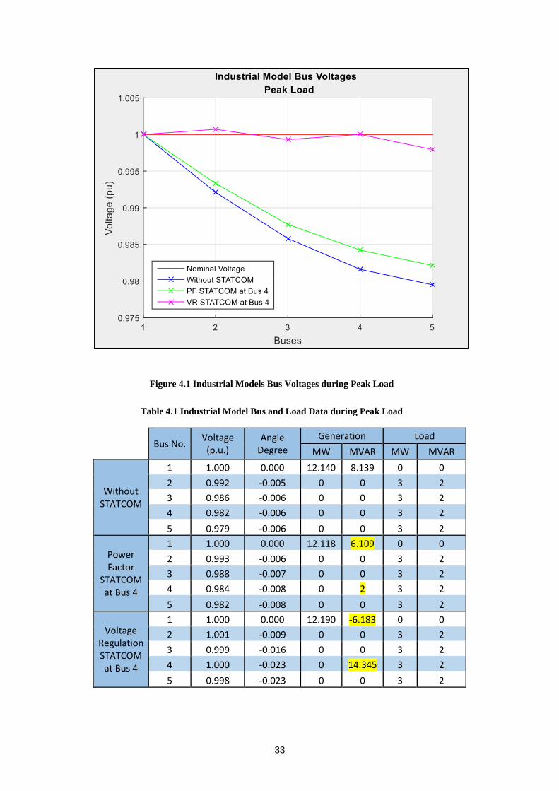
4.1.1 Industrial Modelled Systems during Peak Load
In the case where a STATCOM was installed at Bus 4 for Power Factor Correction
the voltage drops from Bus 1 to 4 was reduced by 0.26 %, this is an improvement
of 14.27 %. A reduction can also be seen for the other load buses upstream and
downstream. The power factor was improved to unity for Bus 4, but the remaining
load buses power factor remained unchanged. There was also a change in the power
factor of Bus 1 which improved by 0.062, this is due to the reduced reactive power
generation of 2.03 MVArs.
In the second case where a STATCOM was installed at Bus 4 for full VR there was
no voltage drop between Bus 1 to 4, a very significant improvement can also be
seen at all other load buses. The voltage rise on Bus 2 is due to the leakage reactance
of the TX between Buses 1 and 2. The power factor at Bus 4 however was
dramatically affected by increased exportation of reactive power, and became 0.236
leading. This was left off the graph due to it being so far off scale. The power factors
of the remaining load buses were unchanged. The generator on Bus 1 has started to
absorb reactive power instead of supplying and has a leading power factor of 0.892.
33
Figure 4.1 Industrial Models Bus Voltages during Peak Load
Table 4.1 Industrial Model Bus and Load Data during Peak Load
Bus No.
Voltage (p.u.)
Angle Degree
Generation Load
MW MVAR MW MVAR
Without STATCOM
1 1.000 0.000 12.140 8.139 0 0
2 0.992 -0.005 0 0 3 2
3 0.986 -0.006 0 0 3 2
4 0.982 -0.006 0 0 3 2
5 0.979 -0.006 0 0 3 2
Power Factor
STATCOM at Bus 4
1 1.000 0.000 12.118 6.109 0 0
2 0.993 -0.006 0 0 3 2
3 0.988 -0.007 0 0 3 2
4 0.984 -0.008 0 2 3 2
5 0.982 -0.008 0 0 3 2
Voltage Regulation STATCOM at Bus 4
1 1.000 0.000 12.190 -6.183 0 0
2 1.001 -0.009 0 0 3 2
3 0.999 -0.016 0 0 3 2
4 1.000 -0.023 0 14.345 3 2
5 0.998 -0.023 0 0 3 2

34
Figure 4.2 Industrial Models Power Factor during Peak Load
4.1.2 Industrial Modelled Systems during Off-Peak Load
In the case where a STATCOM was installed at Bus 4 for Power Factor Correction
the voltage drops from Bus 1 to 4 was reduced by 0.01 %, this is an improvement
of 9.49 %. A reduction can also be seen for the other load buses upstream and
downstream. The power factor was improved to unity for Bus 4, but the remaining
load buses power factor remained unchanged. There was also a change in the power
factor of Bus 1 which improved by 0.019, this was due to the reduced reactive
power generation by 0.1 MVars.
In the second case where a STATCOM was installed at Bus 4 for full VR there was
no voltage drop between Bus 1 to 4, a very significant improvement can also be
seen at all other load buses. The power factor at Bus 4 however was dramatically
affected by increased exportation of reactive power, and became 0.300 leading.
This was left off the graph due to it being so far off scale. The power factors of the

35
remaining load buses were unchanged. The generator on Bus 1 has started to absorb
reactive power instead of supplying and has a leading power factor of 0.862.
Figure 4.3 Industrial Models Bus Voltages during Off-Peak Load
Table 4.2 Industrial Model Bus and Load Data during Off-Peak Load
Bus No.
Voltage (p.u.)
Angle Degree
Generation Load
MW MVAR MW MVAR
Without STATCOM
1 1.000 0.000 1.201 0.347 0 0
2 0.999 -0.001 0 0 0.3 0.1
3 0.999 -0.001 0 0 0.3 0.1
4 0.999 -0.001 0 0 0.3 0.1
5 0.998 -0.001 0 0 0.3 0.1
Power Factor
STATCOM at Bus 4
1 1.000 0.000 1.201 0.247 0 0
2 1.000 -0.001 0 0 0.3 0.1
3 0.999 -0.001 0 0 0.3 0.1
4 0.999 -0.001 0 0.1 0.3 0.1
5 0.999 -0.001 0 0 0.3 0.1
Voltage Regulation STATCOM at Bus 4
1 1.000 0.000 1.202 -0.708 0 0
2 1.000 -0.001 0 0 0.3 0.1
3 1.000 -0.002 0 0 0.3 0.1
4 1.000 -0.002 0 1.055 0.3 0.1
5 1.000 -0.002 0 0 0.3 0.1
36
Figure 4.4 Industrial Models Power Factor during Off-Peak Load
4.1.3 Commercial Modelled Systems Peak Load
In the case where a STATCOM was installed at Bus 4 for Power Factor Correction
the voltage drops from Bus 1 to 4 was reduced by 0.08 %, this is an improvement
of 11.81 %. A reduction can also be seen for the other load buses upstream and
downstream. The power factor was improved to unity for Bus 4, but the remaining
load buses power factor remained unchanged. There was also a change in the power
factor of Bus 1 which improved by 0.093, this was due to the reduced reactive
power generation of 0.70 MVars.
In the second case where a STATCOM was installed at Bus 4 for full VR there was
no voltage drop between Bus 1 to 4, a very significant improvement can also be
seen at all other load buses. The power factor at Bus 4 however was dramatically
affected by increased exportation of reactive power, and became 0.274 leading.
This was left off the graph due to it being so far off scale. The power factors of the
37
remaining load buses were unchanged. The generator on Bus 1 has started to absorb
reactive power instead of supplying and has a leading power factor of 0.885.
Figure 4.5 Commercial Models Bus Voltages during Peak Load
Table 4.3 Commercial Model Bus and Load Data during Peak Load
Bus No.
Voltage (p.u.)
Angle Degree
Generation Load
MW MVAR MW MVAR
Without STATCOM
1 1.000 0.000 6.023 2.799 0 0
2 0.997 -0.003 0 0 1.5 0.7
3 0.995 -0.003 0 0 1.5 0.7
4 0.994 -0.004 0 0 1.5 0.7
5 0.993 -0.004 0 0 1.5 0.7
Power Factor
STATCOM at Bus 4
1 1.000 0.000 6.021 2.096 0 0
2 0.997 -0.003 0 0 1.5 0.7
3 0.996 -0.004 0 0 1.5 0.7
4 0.994 -0.004 0 0.7 1.5 0.7
5 0.994 -0.004 0 0 1.5 0.7
Voltage Regulation STATCOM at Bus 4
1 1.000 0.000 6.033 -3.167 0 0
2 1.000 -0.004 0 0 1.5 0.7
3 1.000 -0.007 0 0 1.5 0.7
4 1.000 -0.009 0 5.974 1.5 0.7
5 0.999 -0.009 0 0 1.5 0.7
38
Figure 4.6 Commercial Models Power Factor during Peak Load
4.1.4 Commercial Modelled Systems Off-Peak Load
In the case where a STATCOM was installed at Bus 4 for Power Factor Correction
there was a very slight reduction in the voltage drop from Bus 1 to 4 but this was
less than 0.001% so will be ignored, a reduction can also be seen for the other load
buses upstream and downstream. The power factor was improved to unity for Bus
4, but the remaining load buses power factor remained unchanged. There was also
a change in the power factor of Bus 1 which improved by 0.0002, this was due to
the reduced reactive power generation of 0.02 MVars.
In the second case where a STATCOM was installed at Bus 4 for full VR there was
no voltage drop between Bus 1 to 4, an improvement can also be seen at all other
load buses. The power factor at Bus 4 however was dramatically affected by
increased exportation of reactive power, and became 0.377 leading. This was left
off the graph due to it being so far off scale. The power factors of the remaining
39
load buses were unchanged. The generator on Bus 1 has started to absorb reactive
power instead of supplying and has a leading power factor of 0.858.
Figure 4.7 Commercial Models Bus Voltages during Off-Peak Load
Table 4.4 Commercial Model Bus and Load Data during Off-Peak Load
Bus No.
Voltage (p.u.)
Angle Degree
Generation Load
MW MVAR MW MVAR
Without STATCOM
1 1.000 0.000 2.002 0.047 0 0
2 0.999 -0.001 0 0 0.5 0.02
3 0.999 -0.002 0 0 0.5 0.02
4 0.999 -0.002 0 0 0.5 0.02
5 0.999 -0.002 0 0 0.5 0.02
Power Factor
STATCOM at Bus 4
1 1.000 0.000 2.002 0.027 0 0
2 0.999 -0.001 0 0 0.5 0.02
3 0.999 -0.002 0 0 0.5 0.02
4 0.999 -0.002 0 0.02 0.5 0.02
5 0.999 -0.002 0 0 0.5 0.02
Voltage Regulation STATCOM at Bus 4
1 1.000 0.000 2.003 -1.200 0 0
2 1.000 -0.002 0 0 0.5 0.02
3 1.000 -0.002 0 0 0.5 0.02
4 1.000 -0.003 0 1.249 0.5 0.02
5 1.000 -0.003 0 0 0.5 0.02
40
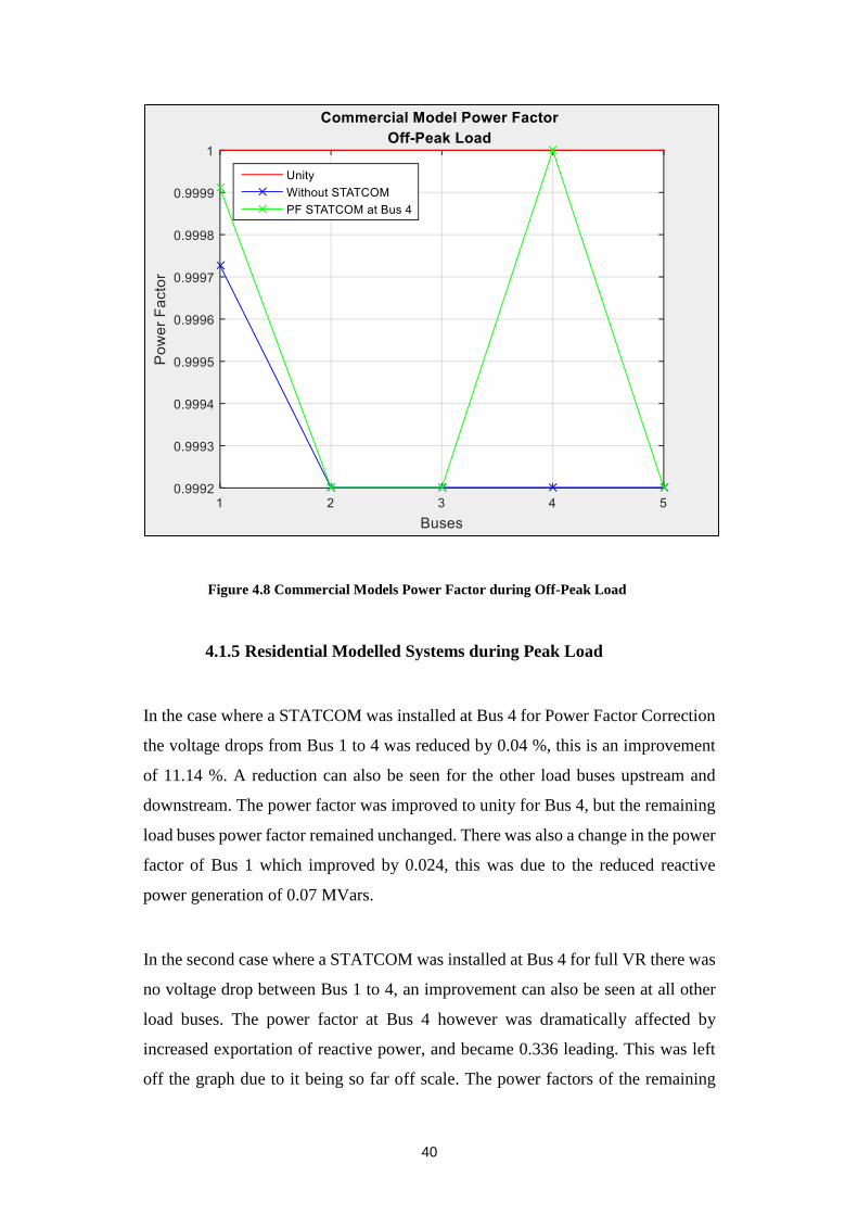
Figure 4.8 Commercial Models Power Factor during Off-Peak Load
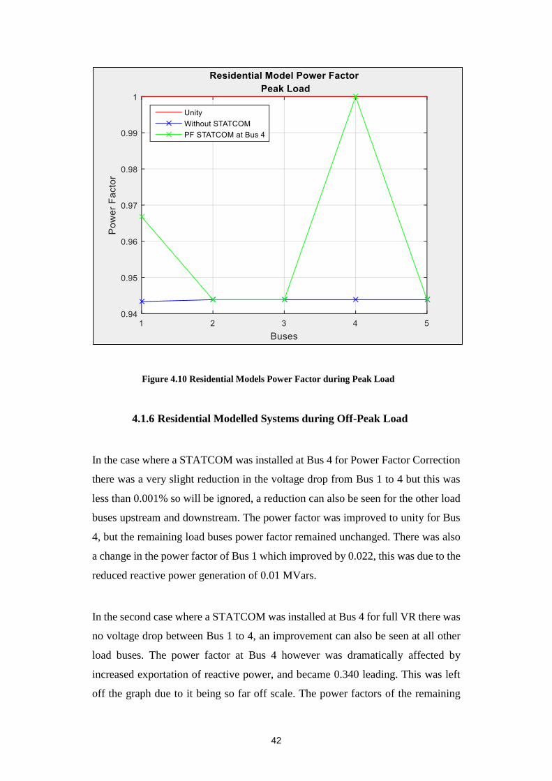
4.1.5 Residential Modelled Systems during Peak Load
In the case where a STATCOM was installed at Bus 4 for Power Factor Correction
the voltage drops from Bus 1 to 4 was reduced by 0.04 %, this is an improvement
of 11.14 %. A reduction can also be seen for the other load buses upstream and
downstream. The power factor was improved to unity for Bus 4, but the remaining
load buses power factor remained unchanged. There was also a change in the power
factor of Bus 1 which improved by 0.024, this was due to the reduced reactive
power generation of 0.07 MVars.
In the second case where a STATCOM was installed at Bus 4 for full VR there was
no voltage drop between Bus 1 to 4, an improvement can also be seen at all other
load buses. The power factor at Bus 4 however was dramatically affected by
increased exportation of reactive power, and became 0.336 leading. This was left
off the graph due to it being so far off scale. The power factors of the remaining
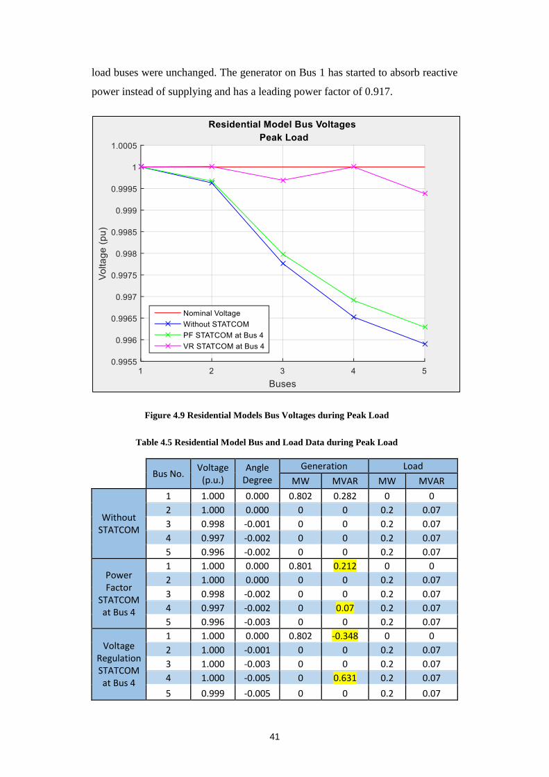
41
load buses were unchanged. The generator on Bus 1 has started to absorb reactive
power instead of supplying and has a leading power factor of 0.917.
Figure 4.9 Residential Models Bus Voltages during Peak Load
Table 4.5 Residential Model Bus and Load Data during Peak Load
Bus No.
Voltage (p.u.)
Angle Degree
Generation Load
MW MVAR MW MVAR
Without STATCOM
1 1.000 0.000 0.802 0.282 0 0
2 1.000 0.000 0 0 0.2 0.07
3 0.998 -0.001 0 0 0.2 0.07
4 0.997 -0.002 0 0 0.2 0.07
5 0.996 -0.002 0 0 0.2 0.07
Power Factor
STATCOM at Bus 4
1 1.000 0.000 0.801 0.212 0 0
2 1.000 0.000 0 0 0.2 0.07
3 0.998 -0.002 0 0 0.2 0.07
4 0.997 -0.002 0 0.07 0.2 0.07
5 0.996 -0.003 0 0 0.2 0.07
Voltage Regulation STATCOM at Bus 4
1 1.000 0.000 0.802 -0.348 0 0
2 1.000 -0.001 0 0 0.2 0.07
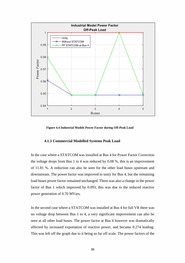
3 1.000 -0.003 0 0 0.2 0.07
4 1.000 -0.005 0 0.631 0.2 0.07
5 0.999 -0.005 0 0 0.2 0.07
42
Figure 4.10 Residential Models Power Factor during Peak Load
4.1.6 Residential Modelled Systems during Off-Peak Load
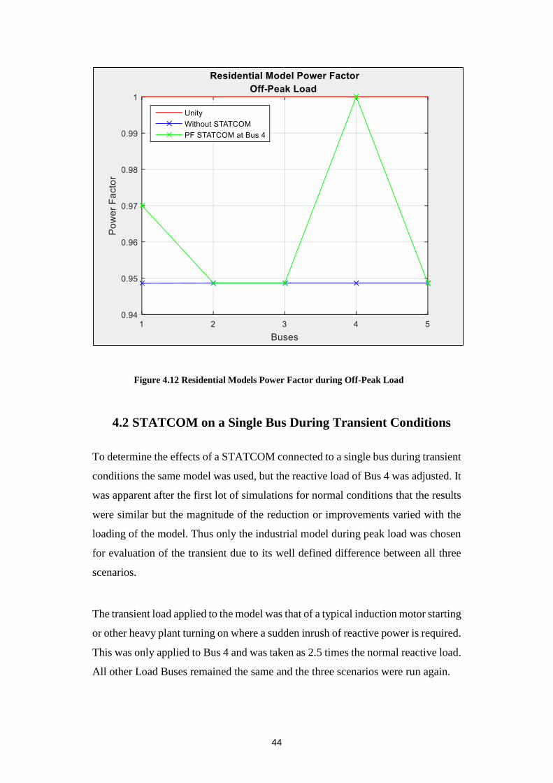
In the case where a STATCOM was installed at Bus 4 for Power Factor Correction
there was a very slight reduction in the voltage drop from Bus 1 to 4 but this was
less than 0.001% so will be ignored, a reduction can also be seen for the other load
buses upstream and downstream. The power factor was improved to unity for Bus
4, but the remaining load buses power factor remained unchanged. There was also
a change in the power factor of Bus 1 which improved by 0.022, this was due to the
reduced reactive power generation of 0.01 MVars.
In the second case where a STATCOM was installed at Bus 4 for full VR there was
no voltage drop between Bus 1 to 4, an improvement can also be seen at all other
load buses. The power factor at Bus 4 however was dramatically affected by
increased exportation of reactive power, and became 0.340 leading. This was left
off the graph due to it being so far off scale. The power factors of the remaining
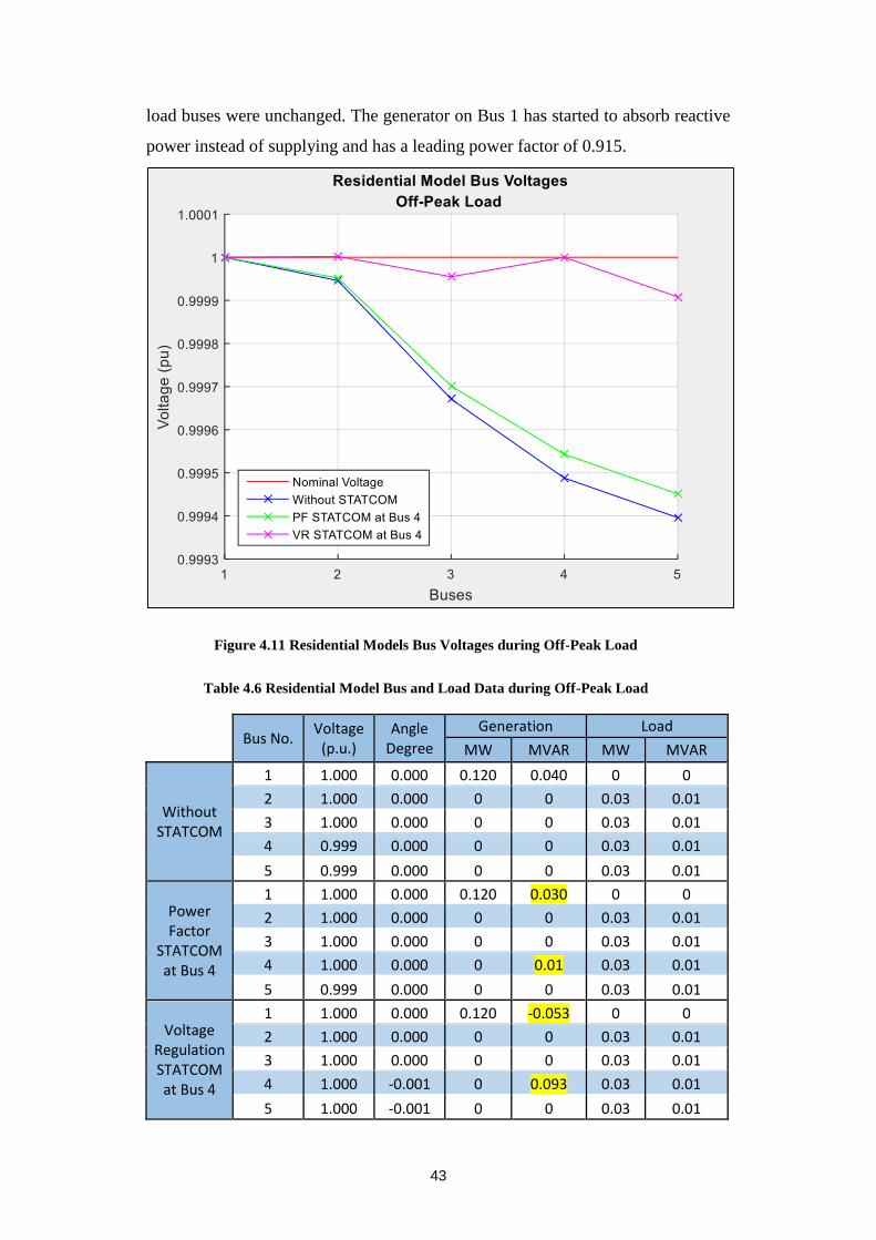
43
load buses were unchanged. The generator on Bus 1 has started to absorb reactive
power instead of supplying and has a leading power factor of 0.915.
Figure 4.11 Residential Models Bus Voltages during Off-Peak Load
Table 4.6 Residential Model Bus and Load Data during Off-Peak Load
Bus No.
Voltage (p.u.)
Angle Degree
Generation Load
MW MVAR MW MVAR
Without STATCOM
1 1.000 0.000 0.120 0.040 0 0
2 1.000 0.000 0 0 0.03 0.01
3 1.000 0.000 0 0 0.03 0.01
4 0.999 0.000 0 0 0.03 0.01
5 0.999 0.000 0 0 0.03 0.01
Power Factor
STATCOM at Bus 4
1 1.000 0.000 0.120 0.030 0 0
2 1.000 0.000 0 0 0.03 0.01
3 1.000 0.000 0 0 0.03 0.01
4 1.000 0.000 0 0.01 0.03 0.01
5 0.999 0.000 0 0 0.03 0.01
Voltage Regulation STATCOM at Bus 4
1 1.000 0.000 0.120 -0.053 0 0
2 1.000 0.000 0 0 0.03 0.01
3 1.000 0.000 0 0 0.03 0.01
4 1.000 -0.001 0 0.093 0.03 0.01
5 1.000 -0.001 0 0 0.03 0.01
44
Figure 4.12 Residential Models Power Factor during Off-Peak Load
4.2 STATCOM on a Single Bus During Transient Conditions
To determine the effects of a STATCOM connected to a single bus during transient
conditions the same model was used, but the reactive load of Bus 4 was adjusted. It
was apparent after the first lot of simulations for normal conditions that the results
were similar but the magnitude of the reduction or improvements varied with the
loading of the model. Thus only the industrial model during peak load was chosen
for evaluation of the transient due to its well defined difference between all three
scenarios.
The transient load applied to the model was that of a typical induction motor starting
or other heavy plant turning on where a sudden inrush of reactive power is required.
This was only applied to Bus 4 and was taken as 2.5 times the normal reactive load.
All other Load Buses remained the same and the three scenarios were run again.

45
In the case where a STATCOM was installed at Bus 4 for Power Factor Correction
the voltage drops from Bus 1 to 4 was reduced by 2.24 %, this is an improvement
of 29.51 %. A reduction can also be seen for the other load buses upstream and
downstream. The power factor was improved to unity for Bus 4, this is a quite
significant improvement of 0.486 from the scenario where no STACOM was
installed. The remaining load buses power factor remained unchanged, but there
was also a change in the power factor of Bus 1 which improved by 0.157, this was
due to the reduced reactive power generation of 5.09 MVars during the transient
condition.
In the second case where a STATCOM was installed at Bus 4 for full VR there was
no voltage drop between Bus 1 to 4, an improvement can also be seen at all other
load buses. The power factor at Bus 4 however was dramatically affected by
increased exportation of reactive power, and became 0.236 leading. This was left
off the graph due to it being so far off scale. The power factors of the remaining
load buses were unchanged. The generator on Bus 1 has started to absorb reactive
power instead of supplying and has a leading power factor of 0.892.

46
Figure 4.13 Industrial Model Bus Voltage during Transient Condition
Table 4.7 Industrial Model Bus and Load Data during Transient Conditions
Bus No.
Voltage (p.u.)
Angle Degree
Generation Load
MW MVAR MW MVAR
Without STATCOM
1 1.000 0.000 12.194 11.203 0 0
2 0.990 -0.005 0 0 3 2
3 0.983 -0.003 0 0 3 2
4 0.978 -0.002 0 0 3 5
5 0.975 -0.002 0 0 3 2
Power Factor
STATCOM at Bus 4
1 1.000 0.000 12.118 6.109 0 0
2 0.993 -0.006 0 0 3 2
3 0.988 -0.007 0 0 3 2
4 0.984 -0.008 0 5 3 5
5 0.982 -0.008 0 0 3 2
Voltage Regulation STATCOM at Bus 4
1 1.000 0.000 12.190 -6.183 0 0
2 1.001 -0.009 0 0 3 2
3 0.999 -0.016 0 0 3 2
4 1.000 -0.023 0 17.345 3 5
5 0.998 -0.023 0 0 3 2

47
Figure 4.14 Industrial Model Power Factor during Transient Condition

48
DISCUSSION AND IMPLICATIONS
5.1 STATCOM used for Power Factor Improvement
In the MATLAB simulations conducted, the STATCOM proved to be effective at
improving the Power Factor not only at the Load Bus that it was installed, but also
at the Bus 1 where the generator was connected to. The performance of the
STATCOM would be limited by the rating, and as such if a customer was installing
a STATCOM it would be best if a power survey was first carried out to discover
their reactive power requirements. A STATCOM that was able to fully improve
their power factor to unity might not be necessary or most economical, as The
Service and Installation Rules of New South Wales currently states that electricity
users must maintain a power factor of 0.9 lagging or above, so improving it beyond
this must be taken on a case by case basis looking at the cost of the equipment and
the savings made from reduced kVAr consumption.
The results from all models clearly showed an improvement in power factor for the
electricity distributor. An improvement for the electricity distributor mean that there
will be less losses associated with transmission, and less reactive power will need
to be generated. This extra capacity means more load can be supplied to future
customers without the need for upgrading existing equipment. The benefit also
extends to customers upstream and downstream of the installed STATCOM via
reduced voltage drop. Because of this improvement for the distributor and
surrounding customers there may be cause in future for the distributor to provide
further financial incentives to improving an electrical installations power factor
beyond the minimum 0.9 lagging. This would be ideal in the case of residential
customers who currently are not charged for their kVAr consumption, whereby
comparison commercial customers with high loads are.
.
49
5.1.1 Power Factor During Transients
During the second round of simulations conducted, transient conditions were
looked at for the Industrial Model during Peak Load. The performance of the
STATCOM in this simulation is where it excels by comparison to the no
STATCOM scenario. Figure 4.14 shows that during a transient condition the power
factor would drop considerable with no STATCOM installed, this has an adverse
effect not only on the customer at Bus 4 but also on the distributor. By comparison,
when the STATCOM is installed, due to its fast response time it would be able to
react to this load change and supply more reactive power for the short time required.
Again this would also have benefit to the distributor as the reactive load
requirements are been met by the onsite STATCOM, and not needing to be
generated and transmitted.
5.2 STATCOM used for Full Voltage Regulation
MATLAB simulations were also run for when the STATCOM was installed in Full
VR mode. This scenario is where the distributor is able to remotely control the
customers STATCOM and use it for the greater benefit of the electrical system.
Interestingly this would require a much larger rated STATCOM than would
normally be installed by a customer as it would now not only look after the local
installation, but the reactive loads of the surrounding installations also. Figure 5.1
shows the size of STATCOM required for each scenario, in all cases the size
required for full VR exceeds the load requirements by a factor of 7. This would
equate to a large financial investment by the customer to install equipment much
larger than their current load requirements. This would not happen unless there were
financial incentives available from the distributor or government. This could come
in the form of them partially paying for the cost of the STATCOM, or perhaps a
feed in tariff introduced for the reactive power being supplied to the grid.
Another interesting result to come from these simulations was that in all cases the
generator at Bus 1 went from supplying reactive load to absorbing reactive load
when the STATCOM was in VR mode. All the Load Buses reactive requirements
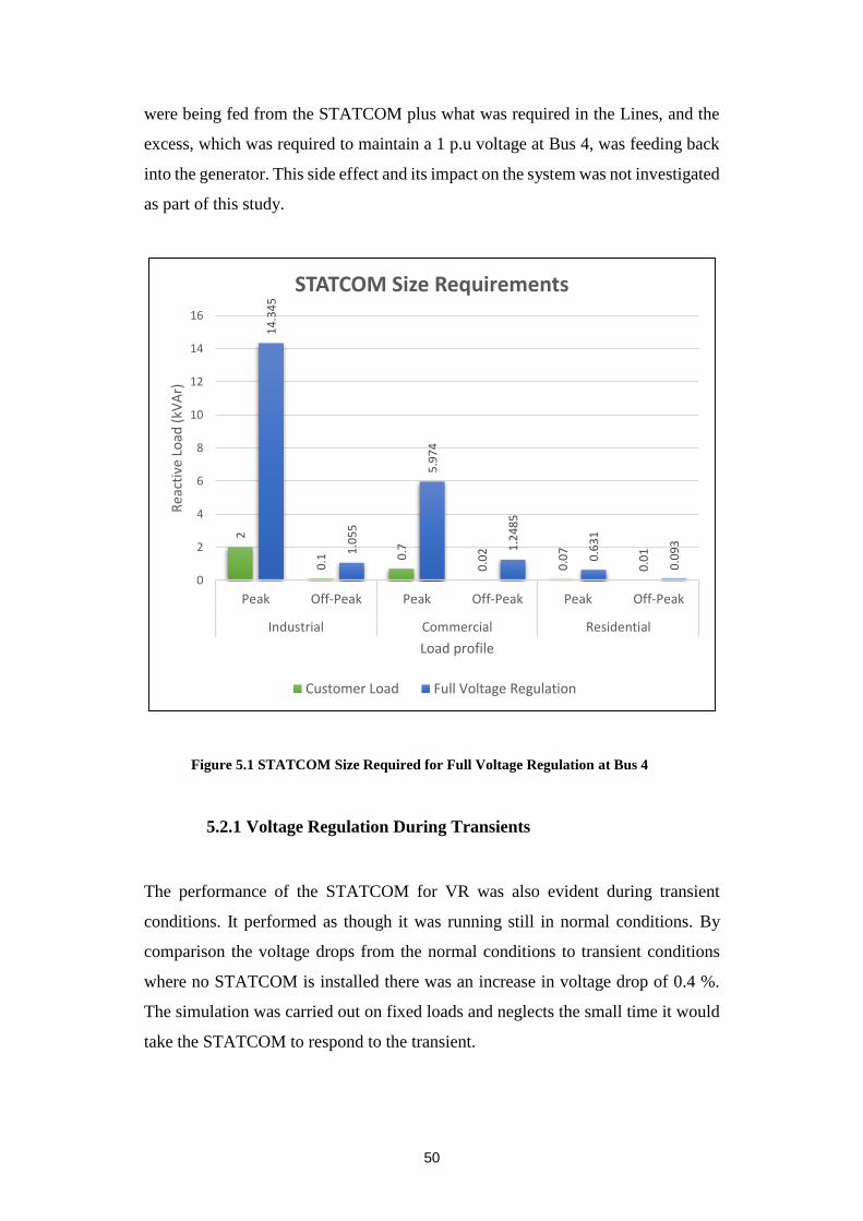
50
were being fed from the STATCOM plus what was required in the Lines, and the
excess, which was required to maintain a 1 p.u voltage at Bus 4, was feeding back
into the generator. This side effect and its impact on the system was not investigated
as part of this study.
Figure 5.1 STATCOM Size Required for Full Voltage Regulation at Bus 4
5.2.1 Voltage Regulation During Transients
The performance of the STATCOM for VR was also evident during transient
conditions. It performed as though it was running still in normal conditions. By
comparison the voltage drops from the normal conditions to transient conditions
where no STATCOM is installed there was an increase in voltage drop of 0.4 %.
The simulation was carried out on fixed loads and neglects the small time it would
take the STATCOM to respond to the transient.
2
0.1 0
.7
0.0
2
0.0
7
0.0
1
14
.34
5
1.0
55
5.9
74
1.2
48
5
0.6
31
0.0
93
0
2
4
6
8
10
12
14
16
Peak Off-Peak Peak Off-Peak Peak Off-Peak
Industrial Commercial Residential
Re
acti
ve L
oad
(kV
Ar)
Load profile
STATCOM Size Requirements
Customer Load Full Voltage Regulation

51
5.3 Compliance with Current Australian Standards
Current Australian Standards (Australia 2015) require that any embedded
generation connected to the electricity grid needs to have the inverters displacement
power factor operating at unity, within the range 0.95 leading to 0.95 lagging.
During my simulations, when the STATCOM was set to power factor correction
mode, it was correcting the whole of the electrical systems power factor to unity,
this required the STATCOM to operate at a power factor well outside this range as
it was solely supplying reactive power and no active power. The worst case was
when the STATCOM was in Full VR mode and supplying in excess of 7 times the
amount of reactive power to the local customer as well as the grid.
The current issue with having inverters suppling at unity is that this reduces the
amount of active power consumed but leaves the systems reactive power
untouched, this puts additional burden on the grid to supply only reactive power to
customers with embedded generation installed. This additional reactive power
means the voltage will rise for the local and surrounding customers.
5.4 Multiple STATCOM Installations
The study has only looked at if there was a single STATCOM installed, some of
the ratings required of the installed STATCOM were unpractically large for a single
customer to installed. A more practical model would be one with multiple
STATCOM installations, that way the burden of reactive power supply could be
shared and the required rating of each could be reduced to a level much closer to
that required by the local installation.
5.5 STATCOM Active and Reactive Power Supply
It is worth mentioning that the simulations performed had the STATCOM inverter
supplying only reactive power. This situation is unlikely as customers who install
solar systems want firstly to generate the power that they will used on site, this
includes both active and reactive power. Unless changes to current standards are

52
made it is also not allowed. Incentives from the government in the form of a reactive
power tariff like the existing active power tariff would increase customers interest
in installing or converting existing inverters to have STATCOM capabilities.
53
CONCLUSIONS
Throughout this project a comprehensive literature review was carried out on
STATCOMs and various techniques surrounding PQ improvement in electrical
systems. Sites were selected for a PQ survey, capturing customers of different load
profiles with PV arrays currently installed. This data was analysed and developed
into a model to be run in MATLAB. Various simulations testing the different modes
the STATCOM could be used for was carried out, including that of the STATCOM
under transient conditions. Benefits pertaining to the installation of a STATCOM
as the inverter for a PV array were discussed in view from both the electricity
distributor and the local customer.
6.1 PQ Improvements using a STATCOM Inverter
VR was found to not only be improved for the location of the installed STATCOM,
but extended to customers upstream and downstream. This improvement was a
direct result of the reduced voltage drop on the system due to the reactive load being
supplied closer to the load and not needing to be transmitted from the generator.
Added benefits to supply being generated closer to the load is the system now has
freed up capacity, this will delay the need for current equipment to be upgraded to
cope with future load growth.
The STATCOM running in Full VR mode case showed that all of the electricity
systems reactive power was needed to be supplied from the Bus where the
STATCOM was installed to bring the voltage level up to 1 p.u. It was also noted
that the generator also went from supplying reactive power to absorbing reactive
power from the STATCOM, this may have undesirable effects and will need to be
further investigated.
The STATCOM running in Power Factor Correction mode showed improvements
only to the Bus where the STATCOM was installed and the generator’s Bus, all

54
other load buses power factor remained unchanged. From a grid perspective it is in
their best interest if all customers were able to operate at close to unity to reduce
the amount of reactive power needed to be generated and transmitted.
As can be seen clearly throughout the study, a STATCOM being installed as the
inverter of a PV array has the ability to supply the reactive power needs of the local
customer. The main beneficiary of this depends on the type of customer load, if it
is for a large industrial customer who is being charge for their kVAr usage then they
will see a financial benefit in reduced electricity bills, whereas residential and small
commercial customers will not as they only pay for their kW consumption. The
electricity distributor was always seen to benefit from a customer installing a
STATCOM, this makes a good case for the distributor to support customers who
want to install STATCOMs via means of a financial incentive or rebate. In the
future energy pricing schemes may change for residential and commercial
customers and they could end up being charged for their kVAr usage, this would
inevitably see an increase in power factor correction equipment such as the
STATCOM on small residential and commercial loads.
6.2 Future Research
This dissertation forms only a small part of the broader study to investigate the
feasibility of converting existing solar inverters to have STATCOM capabilities.
Further study remains in the areas of simulation of a known problem feeder due to
high PV penetration, communications between SMART Meter and SMART Grid,
and a review of current standards relating to inverter requirements.
6.2.1 Investigate feeder with High PV Penetration and VR Issues
The study has provided information regarding a STATCOM installation from a
theoretical standpoint only. There are numerous known feeders currently on the
NSW network that have VR issues resulting from the recent increase of PV
installations. Time constraints meant that a study of one of these feeders could not
be carried out, however future research should involve modelling one of these

55
feeders, preferably in software such as HOMER. The aim should be to convert a
portion, or all of the inverters on the feeder to STATCOMs and investigate and
results on PQ.
6.2.2 Communication between SMART Meter and SMART Grid
Work also remains to research and test communication methods between currently
installed SMART Meters with the electricity grid. A STATCOM is capable of
reading and improving local PQ issues, but a high penetration of STATCOMs all
attempting to fix the same issue, such as maintaining voltage stability, may actually
have a detrimental effect if there was no communication between devices.
Investigation needs to be done into how a SMART Grid could instruct the
STATCOMs to resolve voltage issues efficiently and effectively.
6.2.3 Review of Current Standards for Inverters
This study has outlines constraints that are imposed by current standards on
inverters. The PQ of the model in all scenarios was improved by operating the
STATCOM outside current standards. This study was an extreme approach where
only reactive power was supplied at a power factor of 0. Further study looking into
the optimum power factor for a STATCOM to operate where the benefit was
maximised for both the customer and the electricity grid should be undertaken.
56
REFERENCES
Abu-Sharkh, S, Arnold, RJ, Kohler, J, Li, R, Markvart, T, Ross, JN, Steemers, K,
Wilson, P & Yao, R 2006, 'Can microgrids make a major contribution to UK energy
supply?', Renewable and Sustainable Energy Reviews, vol. 10, no. 2, pp. 78-127.
Ali, SS, Maroof, M & Hanif, S 2010, 'Smart energy meters for energy conservation
& minimizing errors', in 2010 Joint International Conference on Power
Electronics, Drives and Energy Systems, PEDES 2010 and 2010 Power India,
http://www.scopus.com/inward/record.url?eid=2-s2.0-
79952732134&partnerID=40&md5=26a27ff54018bbd6cb5bdb1c9bc275bb
Anders, S 2015, Half-Empty Planes: Utilization Rates for California’s Electric
Grid Part II, viewed 11/07/2016, <https://epicenergyblog.com/2015/07/14/half-
empty-planes-utilization-rates-for-californias-electric-grid-part-ii/>.
Australia, S 2015, AS/NZS 4777.2 Grid connection of energy systems via inverters
Part 2: Inverter requirements, Standards Australia.
Bhattacharya, S, Saha, T & Hossain, MJ 2013, 'Fault current contribution from
photovoltaic systems in residential power networks', in 2013 Australasian
Universities Power Engineering Conference, AUPEC 2013,
http://www.scopus.com/inward/record.url?eid=2-s2.0-
84894468910&partnerID=40&md5=acbc51a53dafaeb72e57a9d0f2bd7cc9>.
Chidurala, A, Saha, TK & Mithulananthan, N 2013, 'Power quality enhancement in
unbalanced distribution network using Solar-DSTATCOM', in Power Engineering
Conference (AUPEC), 2013 Australasian Universities, pp. 1-6.
Council, ITI 2000, ITI Curve (formerly CBEMA), viewed 18/08/2016,
<http://www.powerqualityworld.com/2011/04/itic-power-acceptability-
curve.html>.

57
Dapu, Z, Yixin, N, Jin, Z & Chen, S 2005, 'Reactive Power and Voltage Control in
Deregulated Environment', in Transmission and Distribution Conference and
Exhibition: Asia and Pacific, 2005 IEEE/PES, pp. 1-5.
De Capua, C, Lipari, G, Lugara, M & Morello, R 2014, 'A smart energy meter for
power grids', in Instrumentation and Measurement Technology Conference
(I2MTC) Proceedings, 2014 IEEE International, pp. 878-83.
Elphick, S & Smith, V 2010, 'The 230 V CBEMA curve — Preliminary
studies', in Universities Power Engineering Conference (AUPEC), 2010 20th
Australasian, pp. 1-6.
Escobar, G, Stankovic, AM & Mattavelli, P 2000, 'Reactive power and unbalance
compensation using STATCOM with dissipativity-based control', in Industry
Applications Conference, 2000. Conference Record of the 2000 IEEE, pp. 2058-
65 vol.4.
Henderson, RD & Rose, PJ 1993, 'Harmonics: the effects on power quality and
transformers', in Textile, Fiber and Film Industry Technical Conference, 1993.,
IEEE 1993 Annual, pp. 4/1-411.
Junbiao, H, Khushalani-Solanki, S, Solanki, J & Schoene, J 2012, 'Study of unified
control of STATCOM to resolve the Power quality issues of a grid-connected three
phase PV system', in Innovative Smart Grid Technologies (ISGT), 2012 IEEE PES,
pp. 1-7.
Kirawanich, P & O'Connell, RM 2000, 'Potential harmonic impact of a residential
utility-interactive photovoltaic system', in Harmonics and Quality of Power, 2000.
Proceedings. Ninth International Conference on, pp. 983-7 vol.3,
http://ieeexplore.ieee.org/xpl/articleDetails.jsp?arnumber=896862>.

58
Molderink, A, Bakker, V, Bosman, MGC, Hurink, JL & Smit, GJM 2010,
'Management and Control of Domestic Smart Grid Technology', Smart Grid, IEEE
Transactions on, vol. 1, no. 2, pp. 109-19.
Petoussis, SG, Zhang, XP, Petoussis, AG & Godfrey, KR 2006, 'The Impact of
Reactive Power on the Electricity Market Equilibrium', in Power Systems
Conference and Exposition, 2006. PSCE '06. 2006 IEEE PES, pp. 96-102.
Rao, P, Crow, ML & Yang, Z 2000, 'STATCOM control for power system voltage
control applications', IEEE Transactions on Power Delivery, vol. 15, no. 4, pp.
1311-7.
Reid, WE 1994, 'Power quality issues-standards and guidelines', in Pulp and Paper
Industry Technical Conference, 1994., Conference Record of 1994 Annual, pp.
108-15.
Sen, KK 1999, 'STATCOM - STATic synchronous COMpensator: Theory,
modeling, and applications', in IEEE Engineering Society, Winter Meeting, pp.
1177-83, http://www.scopus.com/inward/record.url?eid=2-s2.0-
0032647271&partnerID=40&md5=ffe247ad50563709344d778448d5f849>.
Solar, W 2016, viewed 29/9/16, <http://www.wholesalesolar.com/solar-
information/start-here/gridtie-information>.
Standards, A 2011, 61000.3.100: Electromagnetic compatibility (EMC), Part 3.100:
Limits—Steady state voltagelimits in public electricity systems.
Tanaka, K, Senjyu, T, Toma, S, Yona, A, Funabashi, T & Chul-Hwan, K 2009,
'Decentralized voltage control in distribution systems by controlling reactive power
of inverters', in Industrial Electronics, 2009. ISIE 2009. IEEE International
Symposium on, pp. 1385-90.

59
Toodeji, H, Farokhnia, N & Riahy, GH 2009, 'Integration of PV module and
STATCOM to extract maximum power from PV', in Electric Power and Energy
Conversion Systems, 2009. EPECS '09. International Conference on, pp. 1-6.
University, SB 2016, Distributed Energy Resources Customer Adoption Model,
viewed 30/09/2016, <https://www.bnl.gov/SET/DER-CAM.php>.

60
APPENDICES
Appendix A - Project Specification

61
University of Southern Queensland
FACULTY OF ENGINEERING AND SURVEYING
ENG4111/4112 Research Project
Project Specification
For: Phillip Nicholson
Title: Power Factor Improvement Using a STATCOM Inverter
Major: Electrical Engineering – Power Engineering
Supervisors: Dr Les Bowtell
Sponsorship: Nil
Enrolment: ENG4111 – EXT S1, 2016
ENG4112 – EXT S2, 2016
Project Aim: To investigate the impact a STATCOM inverter can have on
improving load power factor for commercial and high density
residential loads.
Programme: Issue A, 10th March, 2016
1. Research background information relating to Power Quality.
2. Perform a load survey of a commercial and high density residential load.
3. Analyse load data and develop a system model for use in MATLAB.
4. Evaluate the transient capabilities of a STATCOM inverter on the system
loads modelled in MATLAB.
5. Report on the potential benefits that can be expected to both the consumer
and electricity distributor from a locally installed STATCOM.
If time and resources permit:
6. Carry out laboratory testing of a STATCOM inverter improving a loads
power factor using data read from a SMART meter.
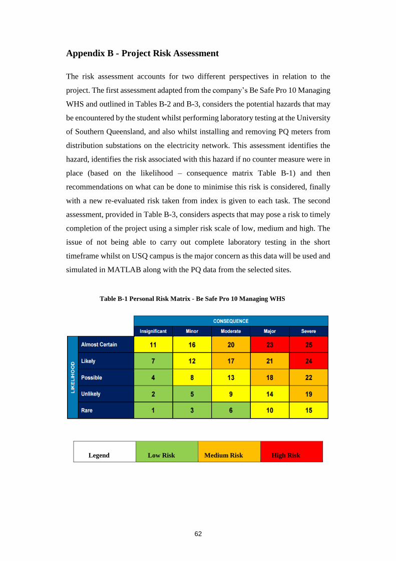
62
Appendix B - Project Risk Assessment
The risk assessment accounts for two different perspectives in relation to the
project. The first assessment adapted from the company’s Be Safe Pro 10 Managing
WHS and outlined in Tables B-2 and B-3, considers the potential hazards that may
be encountered by the student whilst performing laboratory testing at the University
of Southern Queensland, and also whilst installing and removing PQ meters from
distribution substations on the electricity network. This assessment identifies the
hazard, identifies the risk associated with this hazard if no counter measure were in
place (based on the likelihood – consequence matrix Table B-1) and then
recommendations on what can be done to minimise this risk is considered, finally
with a new re-evaluated risk taken from index is given to each task. The second
assessment, provided in Table B-3, considers aspects that may pose a risk to timely
completion of the project using a simpler risk scale of low, medium and high. The
issue of not being able to carry out complete laboratory testing in the short
timeframe whilst on USQ campus is the major concern as this data will be used and
simulated in MATLAB along with the PQ data from the selected sites.
Table B-1 Personal Risk Matrix - Be Safe Pro 10 Managing WHS
Legend Low Risk Medium Risk High Risk
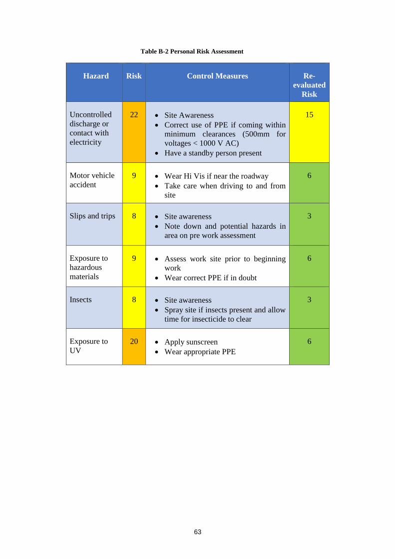
63
Table B-2 Personal Risk Assessment
Hazard Risk Control Measures Re-
evaluated
Risk
Uncontrolled
discharge or
contact with
electricity
22 Site Awareness
Correct use of PPE if coming within
minimum clearances (500mm for
voltages < 1000 V AC)
Have a standby person present
15
Motor vehicle
accident
9 Wear Hi Vis if near the roadway
Take care when driving to and from
site
6
Slips and trips 8 Site awareness
Note down and potential hazards in
area on pre work assessment
3
Exposure to
hazardous
materials
9 Assess work site prior to beginning
work
Wear correct PPE if in doubt
6
Insects 8 Site awareness
Spray site if insects present and allow
time for insecticide to clear
3
Exposure to
UV
20 Apply sunscreen
Wear appropriate PPE
6
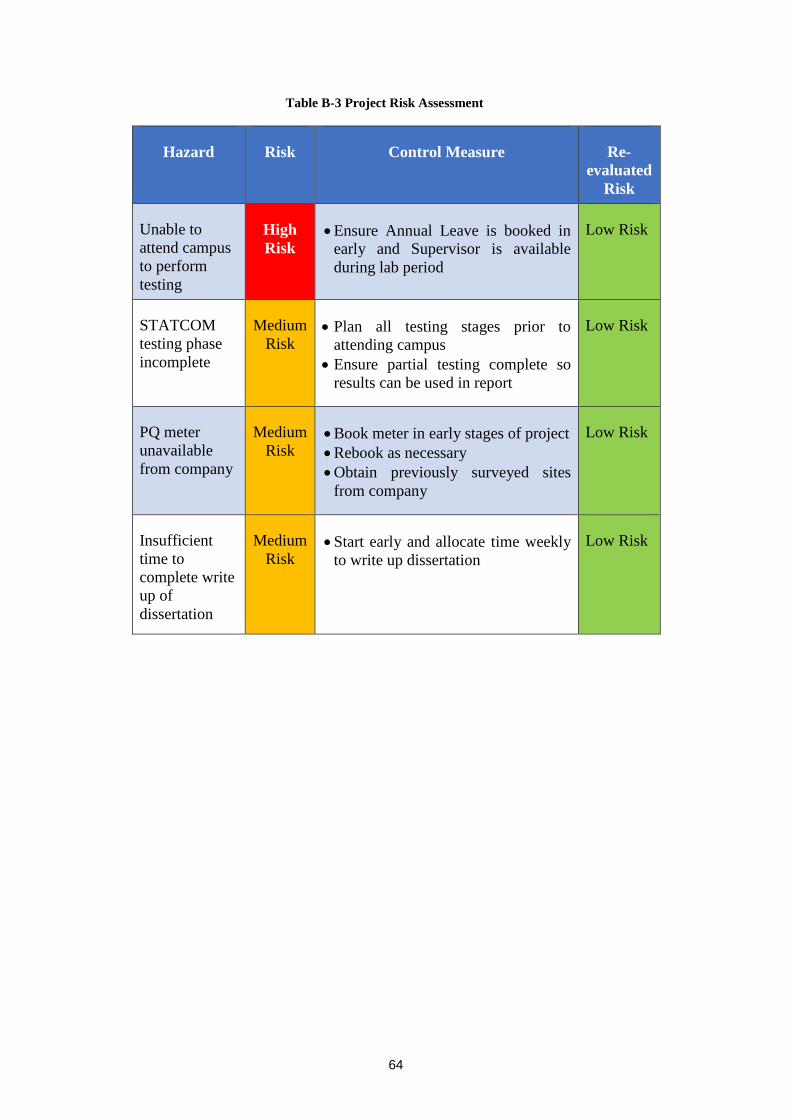
64
Table B-3 Project Risk Assessment
Hazard Risk Control Measure Re-
evaluated
Risk
Unable to
attend campus
to perform
testing
High
Risk Ensure Annual Leave is booked in
early and Supervisor is available
during lab period
Low Risk
STATCOM
testing phase
incomplete
Medium
Risk Plan all testing stages prior to
attending campus
Ensure partial testing complete so
results can be used in report
Low Risk
PQ meter
unavailable
from company
Medium
Risk Book meter in early stages of project
Rebook as necessary
Obtain previously surveyed sites
from company
Low Risk
Insufficient
time to
complete write
up of
dissertation
Medium
Risk Start early and allocate time weekly
to write up dissertation
Low Risk

65
Appendix C - Project Timeline
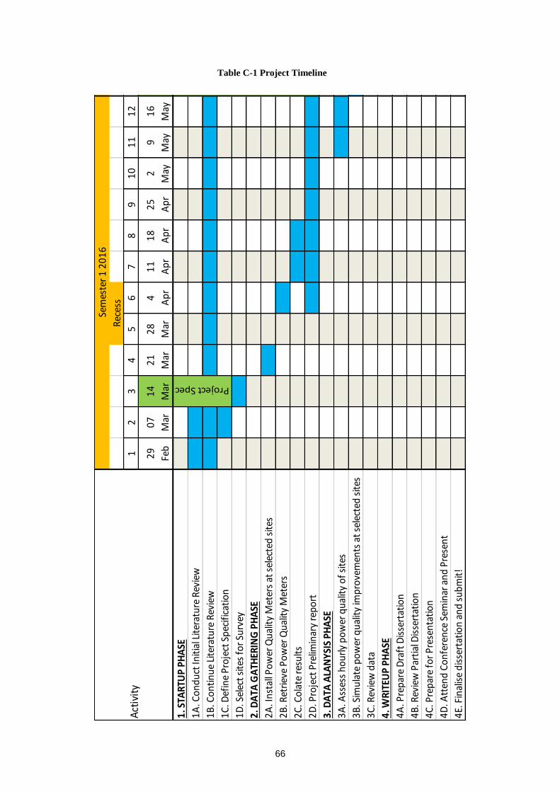
66
Table C-1 Project Timeline
12
34
56
78
91
01
11
2
29
Feb
07
Mar
14
Mar
21
Mar
28
Mar
4 Ap
r
11
Ap
r
18
Ap
r
25
Ap
r
2
May
9
May
16
May
1. S
TAR
TUP
PH
ASE
1A
. Co
nd
uct
Init
ial L
iter
atu
re R
evie
w
1B
. Co
nti
nu
e Li
tera
ture
Rev
iew
1C
. Def
ine
Pro
ject
Sp
ecif
icat
ion
1D
. Sel
ect
site
s fo
r Su
rvey
2. D
ATA
GA
THER
ING
PH
ASE
2A
. In
stal
l Po
wer
Qu
alit
y M
eter
s at
sel
ecte
d s
ites
2B
. Ret
riev
e P
ow
er Q
ual
ity
Met
ers
2C
. Co
late
res
ult
s
2D
. Pro
ject
Pre
limin
ary
rep
ort
3. D
ATA
ALA
NY
SIS
PH
ASE
3A
. Ass
ess
ho
url
y p
ow
er q
ual
ity
of
site
s
3B
. Sim
ula
te p
ow
er q
ual
ity
imp
rove
men
ts a
t se
lect
ed s
ites
3C
. Rev
iew
dat
a
4. W
RIT
EUP
PH
ASE
4A
. Pre
par
e D
raft
Dis
sert
atio
n
4B
. Rev
iew
Par
tial
Dis
sert
atio
n
4C
. Pre
par
e fo
r P
rese
nta
tio
n
4D
. Att
end
Co
nfe
ren
ce S
emin
ar a
nd
Pre
sen
t
4E.
Fin
alis
e d
isse
rtat
ion
an
d s
ub
mit
!
Project Spec
Act
ivit
y
Rec
ess
Sem
este
r 1
20
16
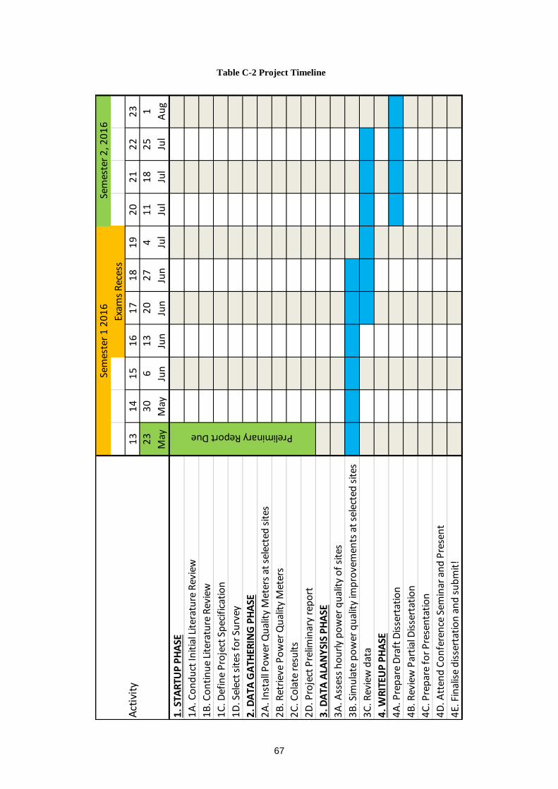
67
Table C-2 Project Timeline
13
14
15
16
17
18
19
20
21
22
23
23
May
30
May
6 Jun
13
Jun
20
Jun
27
Jun
4 Jul
11
Jul
18
Jul
25
Jul
1
Au
g
1. S
TAR
TUP
PH
ASE
1A
. Co
nd
uct
Init
ial L
iter
atu
re R
evie
w
1B
. Co
nti
nu
e Li
tera
ture
Rev
iew
1C
. Def
ine
Pro
ject
Sp
ecif
icat
ion
1D
. Sel
ect
site
s fo
r Su
rvey
2. D
ATA
GA
THER
ING
PH
ASE
2A
. In
stal
l Po
wer
Qu
alit
y M
eter
s at
sel
ecte
d s
ites
2B
. Ret
riev
e P
ow
er Q
ual
ity
Met
ers
2C
. Co
late
res
ult
s
2D
. Pro
ject
Pre
limin
ary
rep
ort
3. D
ATA
ALA
NY
SIS
PH
ASE
3A
. Ass
ess
ho
url
y p
ow
er q
ual
ity
of
site
s
3B
. Sim
ula
te p
ow
er q
ual
ity
imp
rove
men
ts a
t se
lect
ed s
ites
3C
. Rev
iew
dat
a
4. W
RIT
EUP
PH
ASE
4A
. Pre
par
e D
raft
Dis
sert
atio
n
4B
. Rev
iew
Par
tial
Dis
sert
atio
n
4C
. Pre
par
e fo
r P
rese
nta
tio
n
4D
. Att
end
Co
nfe
ren
ce S
emin
ar a
nd
Pre
sen
t
4E.
Fin
alis
e d
isse
rtat
ion
an
d s
ub
mit
!
Act
ivit
yEx
ams
Rec
ess
Preliminary Report Due
Sem
este
r 1
20
16
Sem
este
r 2
, 20
16
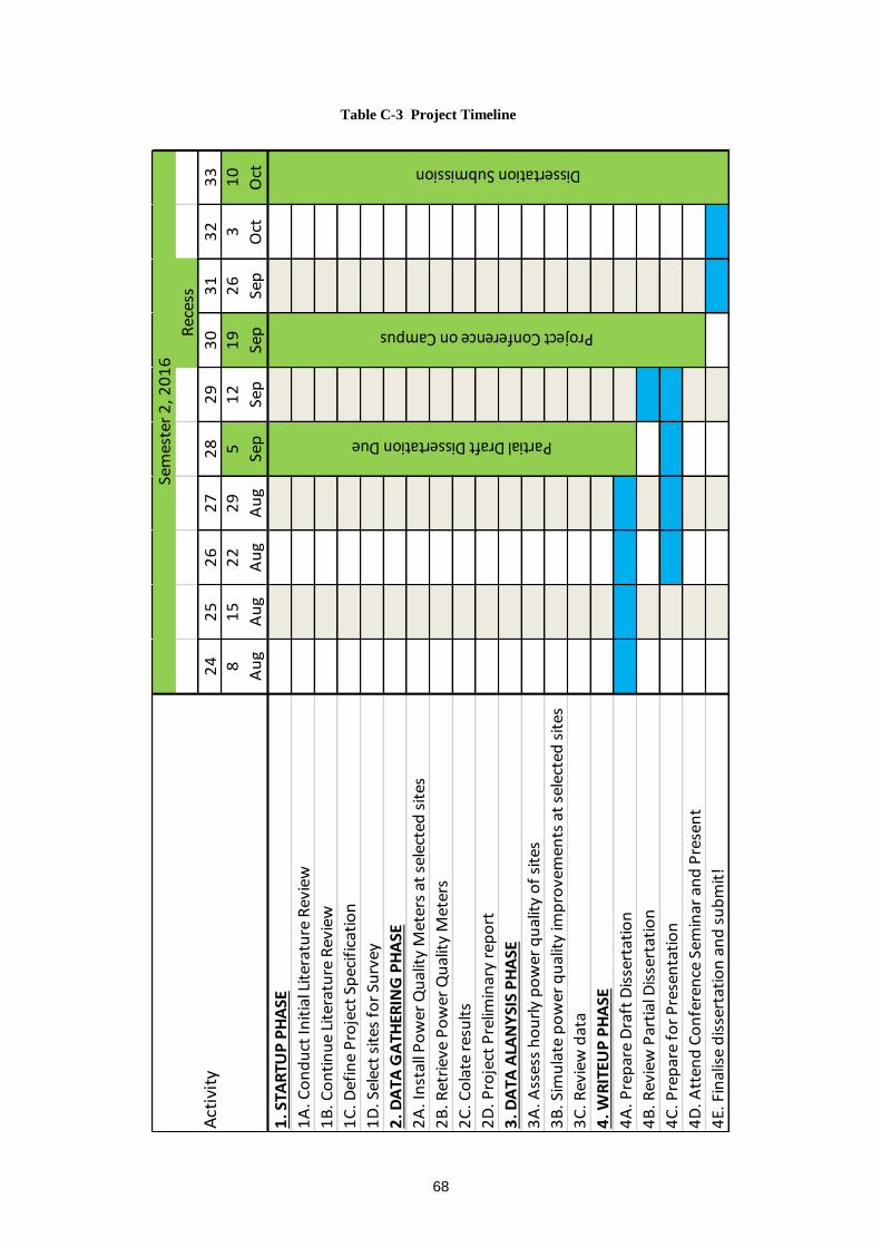
68
Table C-3 Project Timeline
24
25
26
27
28
29
30
31
32
33
8
Au
g
15
Au
g
22
Au
g
29
Au
g
5 Sep
12
Sep
19
Sep
26
Sep
3 Oct
10
Oct
1. S
TAR
TUP
PH
ASE
1A
. Co
nd
uct
Init
ial L
iter
atu
re R
evie
w
1B
. Co
nti
nu
e Li
tera
ture
Rev
iew
1C
. Def
ine
Pro
ject
Sp
ecif
icat
ion
1D
. Sel
ect
site
s fo
r Su
rvey
2. D
ATA
GA
THER
ING
PH
ASE
2A
. In
stal
l Po
wer
Qu
alit
y M
eter
s at
sel
ecte
d s
ites
2B
. Ret
riev
e P
ow
er Q
ual
ity
Met
ers
2C
. Co
late
res
ult
s
2D
. Pro
ject
Pre
limin
ary
rep
ort
3. D
ATA
ALA
NY
SIS
PH
ASE
3A
. Ass
ess
ho
url
y p
ow
er q
ual
ity
of
site
s
3B
. Sim
ula
te p
ow
er q
ual
ity
imp
rove
men
ts a
t se
lect
ed s
ites
3C
. Rev
iew
dat
a
4. W
RIT
EUP
PH
ASE
4A
. Pre
par
e D
raft
Dis
sert
atio
n
4B
. Rev
iew
Par
tial
Dis
sert
atio
n
4C
. Pre
par
e fo
r P
rese
nta
tio
n
4D
. Att
end
Co
nfe
ren
ce S
emin
ar a
nd
Pre
sen
t
4E.
Fin
alis
e d
isse
rtat
ion
an
d s
ub
mit
!
Act
ivit
y
Sem
este
r 2
, 20
16
Rec
ess
Partial Draft Dissertation Due
Project Conference on Campus
Dissertation Submission

69
Appendix D - Resource Requirements
A resource analysis outlining equipment and data requirements for the project is
provided in Tables D-1-3. The majority of resources are available at either the USQ
laboratories or via the company. The company has allowed the use of the PQ
loggers for the purpose of this project. Software has previously been purchased as
part of previous studies at USQ.
Table D-1 Project Resources
Task Item Amount Source Cost Image
2A -
2B
PQ
Logger One (1) Company Nil
2A -
2B
Safety
Gloves Two (2) Company Nil
2A -
2B
Safety
Glasses One (1) Company Nil

70
Table D-2 Project Resources
Task Item Amount Source Cost Image
2A -
2B
Hard
Hat One (1) Company Nil
2A -
2B
Hi-Vis
Shirt One (1) Company Nil
2A -
2B
Heavy
Duty
Pants
One (1) Company Nil
2A -
2B
Safety
Boots Two (2) Company Nil
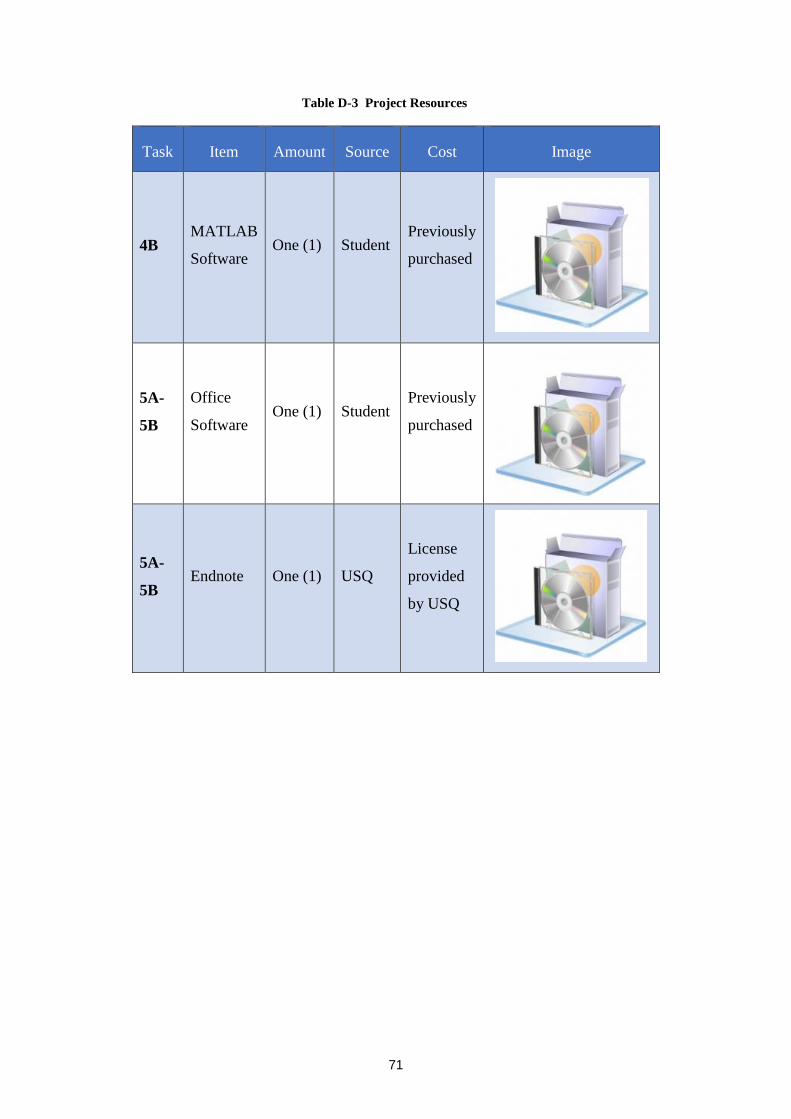
71
Table D-3 Project Resources
Task Item Amount Source Cost Image
4B MATLAB
Software One (1) Student
Previously
purchased
5A-
5B
Office
Software One (1) Student
Previously
purchased
5A-
5B Endnote One (1) USQ
License
provided
by USQ
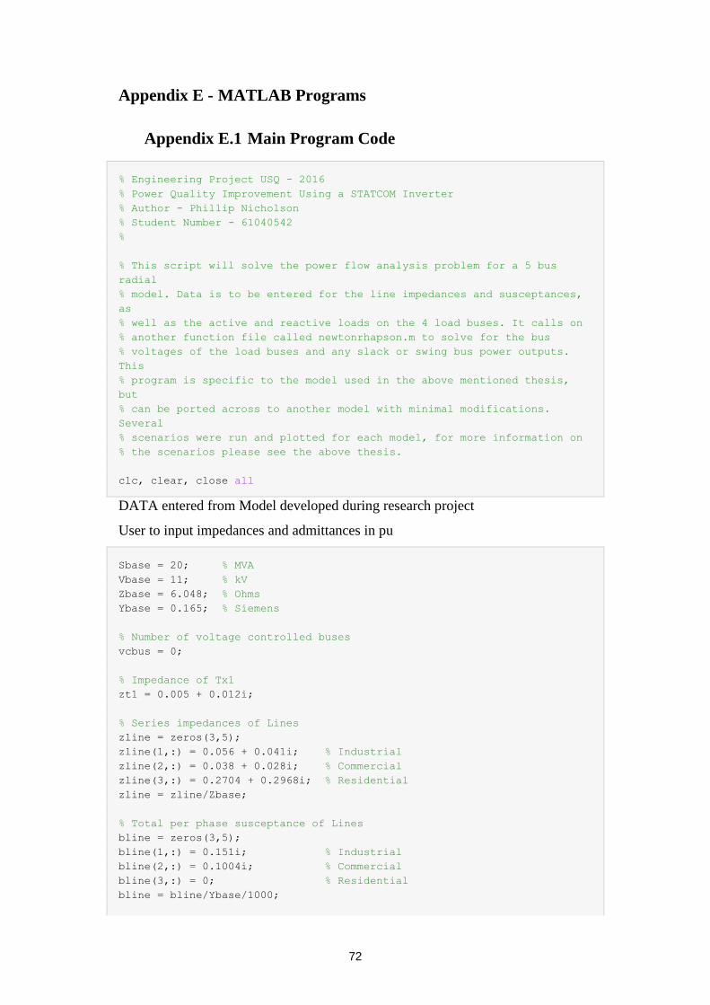
72
Appendix E - MATLAB Programs
Appendix E.1 Main Program Code
% Engineering Project USQ - 2016
% Power Quality Improvement Using a STATCOM Inverter
% Author - Phillip Nicholson
% Student Number - 61040542
%
% This script will solve the power flow analysis problem for a 5 bus
radial
% model. Data is to be entered for the line impedances and susceptances,
as
% well as the active and reactive loads on the 4 load buses. It calls on
% another function file called newtonrhapson.m to solve for the bus
% voltages of the load buses and any slack or swing bus power outputs.
This
% program is specific to the model used in the above mentioned thesis,
but
% can be ported across to another model with minimal modifications.
Several
% scenarios were run and plotted for each model, for more information on
% the scenarios please see the above thesis.
clc, clear, close all
DATA entered from Model developed during research project
User to input impedances and admittances in pu
Sbase = 20; % MVA
Vbase = 11; % kV
Zbase = 6.048; % Ohms
Ybase = 0.165; % Siemens
% Number of voltage controlled buses
vcbus = 0;
% Impedance of Tx1
zt1 = 0.005 + 0.012i;
% Series impedances of Lines
zline = zeros(3,5);
zline(1,:) = 0.056 + 0.041i; % Industrial
zline(2,:) = 0.038 + 0.028i; % Commercial
zline(3,:) = 0.2704 + 0.2968i; % Residential
zline = zline/Zbase;
% Total per phase susceptance of Lines
bline = zeros(3,5);
bline(1,:) = 0.151i; % Industrial
bline(2,:) = 0.1004i; % Commercial
bline(3,:) = 0; % Residential
bline = bline/Ybase/1000;
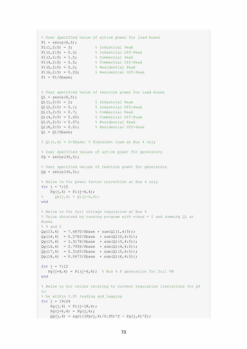
73
% User specified value of active power for load buses
Pl = zeros(6,5);
Pl(1,2:5) = 3; % Industrial Peak
Pl(2,2:5) = 0.3; % Industrial Off-Peak
Pl(3,2:5) = 1.5; % Commercial Peak
Pl(4,2:5) = 0.5; % Commercial Off-Peak
Pl(5,2:5) = 0.2; % Residential Peak
Pl(6,2:5) = 0.03; % Residential Off-Peak
Pl = Pl/Sbase;
% User specified value of reactive power for load buses
Ql = zeros(6,5);
Ql(1,2:5) = 2; % Industrial Peak
Ql(2,2:5) = 0.1; % Industrial Off-Peak
Ql(3,2:5) = 0.7; % Commercial Peak
Ql(4,2:5) = 0.02; % Commercial Off-Peak
Ql(5,2:5) = 0.07; % Residential Peak
Ql(6,2:5) = 0.01; % Residential Off-Peak
Ql = Ql/Sbase;
% Ql(1,4) = 5/Sbase; % Transient load at Bus 4 only
% User specified values of active power for generators
Pg = zeros(30,5);
% User specified values of reactive power for generators
Qg = zeros(30,5);
% Below is for power factor correction at Bus 4 only
for j = 7:12
Pg(j,4) = Pl(j-6,4);
% Qg(j,4) = Ql(j-6,4);
end
% Below is for full voltage regulation at Bus 4
% Value obtained by running program with vcbus = 2 and summing Ql at
Buses
% 4 and 5
Qg(13,4) = 7.4870/Sbase + sum(Ql(1,4:5));
Qg(14,4) = 0.5782/Sbase + sum(Ql(2,4:5));
Qg(15,4) = 3.3178/Sbase + sum(Ql(3,4:5));
Qg(16,4) = 0.7936/Sbase + sum(Ql(4,4:5));
Qg(17,4) = 0.3183/Sbase + sum(Ql(5,4:5));
Qg(18,4) = 0.0473/Sbase + sum(Ql(6,4:5));
for j = 7:12
Pg(j+6,4) = Pl(j-6,4); % Bus 4 P generation for full VR
end
% Below is for values relating to current regulation limitations for pf
to
% be within 0.95 leading and lagging
for j = 19:24
Pg(j,4) = Pl(j-18,4);
Pg(j+6,4) = Pg(j,4);
Qg(j,4) = sqrt((Pg(j,4)/0.95)^2 - Pg(j,4)^2);
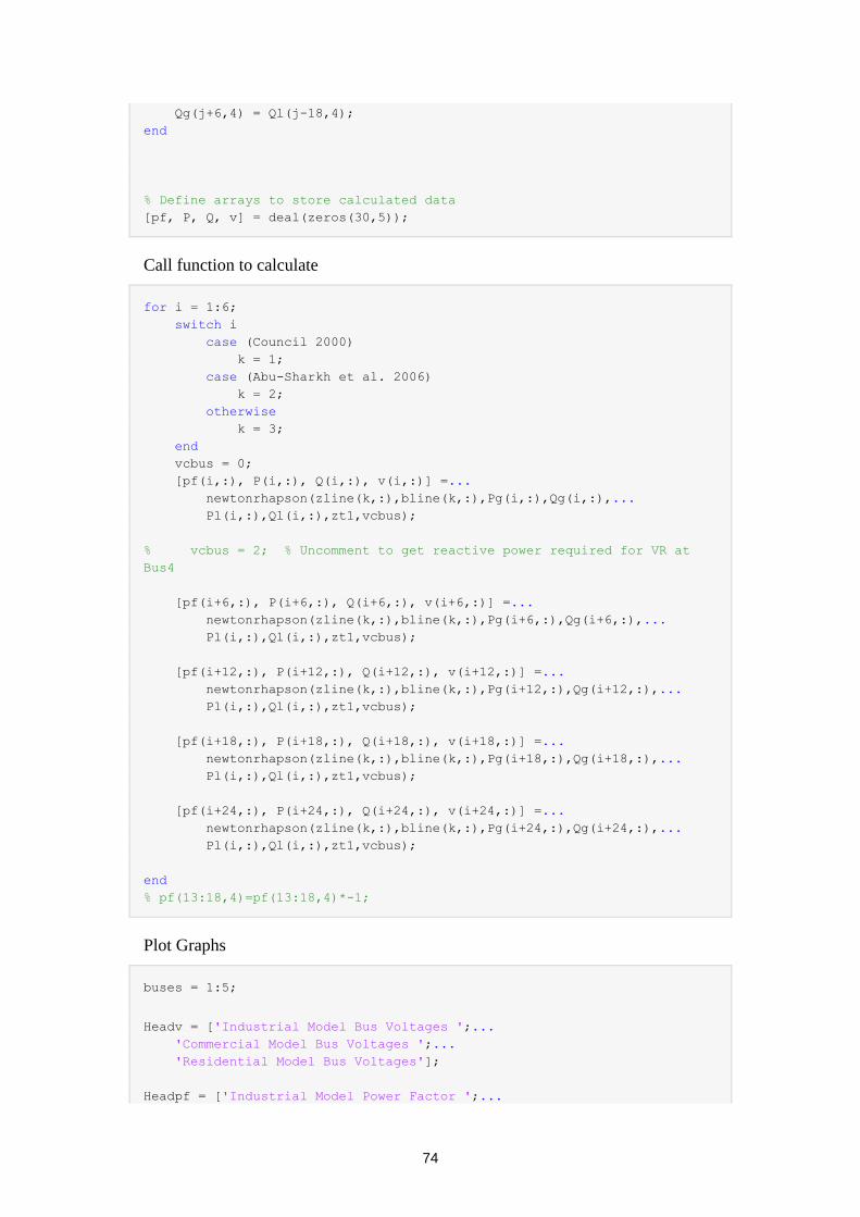
74
Qg(j+6,4) = Ql(j-18,4);
end
% Define arrays to store calculated data
[pf, P, Q, v] = deal(zeros(30,5));
Call function to calculate
for i = 1:6;
switch i
case (Council 2000)
k = 1;
case (Abu-Sharkh et al. 2006)
k = 2;
otherwise
k = 3;
end
vcbus = 0;
[pf(i,:), P(i,:), Q(i,:), v(i,:)] =...
newtonrhapson(zline(k,:),bline(k,:),Pg(i,:),Qg(i,:),...
Pl(i,:),Ql(i,:),zt1,vcbus);
% vcbus = 2; % Uncomment to get reactive power required for VR at
Bus4
[pf(i+6,:), P(i+6,:), Q(i+6,:), v(i+6,:)] =...
newtonrhapson(zline(k,:),bline(k,:),Pg(i+6,:),Qg(i+6,:),...
Pl(i,:),Ql(i,:),zt1,vcbus);
[pf(i+12,:), P(i+12,:), Q(i+12,:), v(i+12,:)] =...
newtonrhapson(zline(k,:),bline(k,:),Pg(i+12,:),Qg(i+12,:),...
Pl(i,:),Ql(i,:),zt1,vcbus);
[pf(i+18,:), P(i+18,:), Q(i+18,:), v(i+18,:)] =...
newtonrhapson(zline(k,:),bline(k,:),Pg(i+18,:),Qg(i+18,:),...
Pl(i,:),Ql(i,:),zt1,vcbus);
[pf(i+24,:), P(i+24,:), Q(i+24,:), v(i+24,:)] =...
newtonrhapson(zline(k,:),bline(k,:),Pg(i+24,:),Qg(i+24,:),...
Pl(i,:),Ql(i,:),zt1,vcbus);
end
% pf(13:18,4)=pf(13:18,4)*-1;
Plot Graphs
buses = 1:5;
Headv = ['Industrial Model Bus Voltages ';...
'Commercial Model Bus Voltages ';...
'Residential Model Bus Voltages'];
Headpf = ['Industrial Model Power Factor ';...
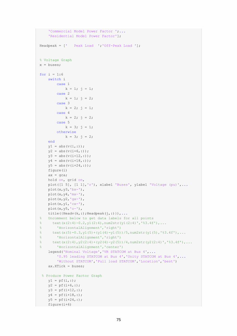
75
'Commercial Model Power Factor ';...
'Residential Model Power Factor'];
Headpeak = [' Peak Load ';'Off-Peak Load '];
% Voltage Graph
x = buses;
for i = 1:6
switch i
case 1
k = 1; j = 1;
case 2
k = 1; j = 2;
case 3
k = 2; j = 1;
case 4
k = 2; j = 2;
case 5
k = 3; j = 1;
otherwise
k = 3; j = 2;
end
y1 = abs(v(i,:));
y2 = abs(v(i+6,:));
y3 = abs(v(i+12,:));
y4 = abs(v(i+18,:));
y5 = abs(v(i+24,:));
figure(i)
ax = gca;
hold on, grid on,
plot([1 5], [1 1],'r'), xlabel 'Buses', ylabel 'Voltage (pu)',...
plot(x,y3,'bx-'),
plot(x,y4,'mx-'),
plot(x,y2,'gx-'),
plot(x,y1,'cx-'),
plot(x,y5,'o-'),
title({Headv(k,:);Headpeak(j,:)}),...
% Uncomment below to get data labels for all points
% text(x(2:4)-0.2,y1(2:4),num2str(y1(2:4)','%3.4f'),...
% 'HorizontalAlignment','right')
% text(x(5)-0.3,y1(5)+(y1(4)-y1(5))/5,num2str(y1(5),'%3.4f'),...
% 'HorizontalAlignment','right')
% text(x(2:4),y2(2:4)+(y2(4)-y2(5))/4,num2str(y2(2:4)','%3.4f'),...
% 'HorizontalAlignment','center')
legend('Nominal Voltage','VR STATCOM at Bus 4',...
'0.95 leading STATCOM at Bus 4','Unity STATCOM at Bus 4',...
'Without STATCOM','Full load STATCOM','Location','best')
ax.XTick = buses;
% Produce Power Factor Graph
y1 = pf(i,:);
y2 = pf(i+6,:);
y3 = pf(i+12,:);
y4 = pf(i+18,:);
y5 = pf(i+24,:);
figure(i+6)
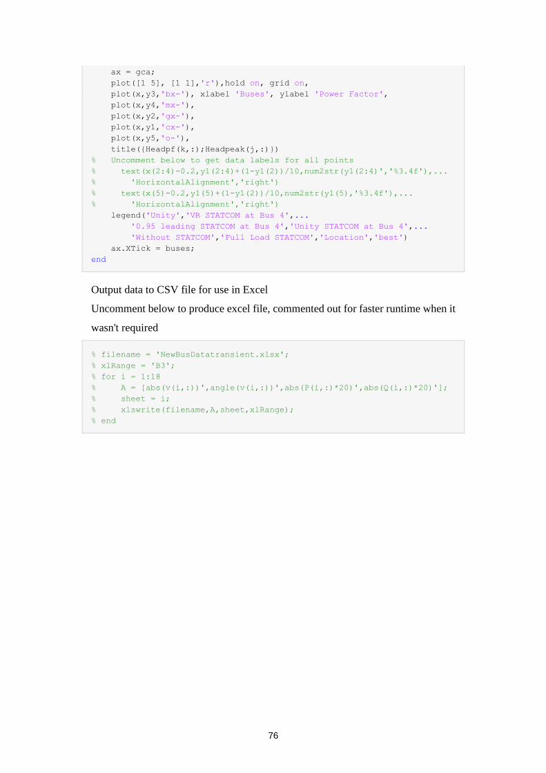
76
ax = gca;
plot([1 5], [1 1],'r'),hold on, grid on,
plot(x,y3,'bx-'), xlabel 'Buses', ylabel 'Power Factor',
plot(x,y4,'mx-'),
plot(x,y2,'gx-'),
plot(x,y1,'cx-'),
plot(x,y5,'o-'),
title({Headpf(k,:);Headpeak(j,:)})
% Uncomment below to get data labels for all points
% text(x(2:4)-0.2,y1(2:4)+(1-y1(2))/10,num2str(y1(2:4)','%3.4f'),...
% 'HorizontalAlignment','right')
% text(x(5)-0.2,y1(5)+(1-y1(2))/10,num2str(y1(5),'%3.4f'),...
% 'HorizontalAlignment','right')
legend('Unity','VR STATCOM at Bus 4',...
'0.95 leading STATCOM at Bus 4','Unity STATCOM at Bus 4',...
'Without STATCOM','Full Load STATCOM','Location','best')
ax.XTick = buses;
end
Output data to CSV file for use in Excel
Uncomment below to produce excel file, commented out for faster runtime when it
wasn't required
% filename = 'NewBusDatatransient.xlsx';
% xlRange = 'B3';
% for i = 1:18
% A = [abs(v(i,:))',angle(v(i,:))',abs(P(i,:)*20)',abs(Q(i,:)*20)'];
% sheet = i;
% xlswrite(filename,A,sheet,xlRange);
% end
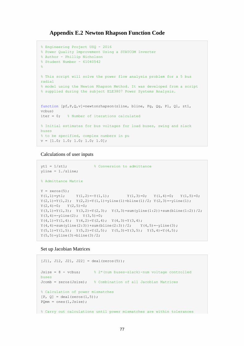
77
Appendix E.2 Newton Rhapson Function Code
% Engineering Project USQ - 2016
% Power Quality Improvement Using a STATCOM Inverter
% Author - Phillip Nicholson
% Student Number - 61040542
%
% This script will solve the power flow analysis problem for a 5 bus
radial
% model using the Newton Rhapson Method. It was developed from a script
% supplied during the subject ELE3807 Power Systems Analysis.
function [pf,P,Q,v]=newtonrhapson(zline, bline, Pg, Qg, Pl, Ql, zt1,
vcbus)
iter = 0; % Number of iterations calculated
% Initial estimates for bus voltages for load buses, swing and slack
buses
% to be specified, complex numbers in pu
v = [1.0; 1.0; 1.0; 1.0; 1.0];
Calculations of user inputs
yt1 = 1/zt1; % Conversion to admittance
yline = 1./zline;
% Admittance Matrix
Y = zeros(5);
Y(1,1)=yt1; Y(1,2)=-Y(1,1); Y(1,3)=0; Y(1,4)=0; Y(1,5)=0;
Y(2,1)=Y(1,2); Y(2,2)=Y(1,1)+yline(1)+bline(1)/2; Y(2,3)=-yline(1);
Y(2,4)=0; Y(2,5)=0;
Y(3,1)=Y(1,3); Y(3,2)=Y(2,3); Y(3,3)=sum(yline(1:2))+sum(bline(1:2))/2;
Y(3,4)=-yline(2); Y(3,5)=0;
Y(4,1)=Y(1,4); Y(4,2)=Y(2,4); Y(4,3)=Y(3,4);
Y(4,4)=sum(yline(2:3))+sum(bline(2:3))/2; Y(4,5)=-yline(3);
Y(5,1)=Y(1,5); Y(5,2)=Y(2,5); Y(5,3)=Y(3,5); Y(5,4)=Y(4,5);
Y(5,5)=yline(3)+bline(3)/2;
Set up Jacobian Matrices
[J11, J12, J21, J22] = deal(zeros(5));
Jsize = 8 - vcbus; % 2*(num buses-slack)-num voltage controlled
buses
Jcomb = zeros(Jsize); % Combination of all Jacobian Matrices
% Calculation of power mismatches
[P, Q] = deal(zeros(1,5));
PQmm = ones(1,Jsize);
% Carry out calculations until power mismatches are within tolerances
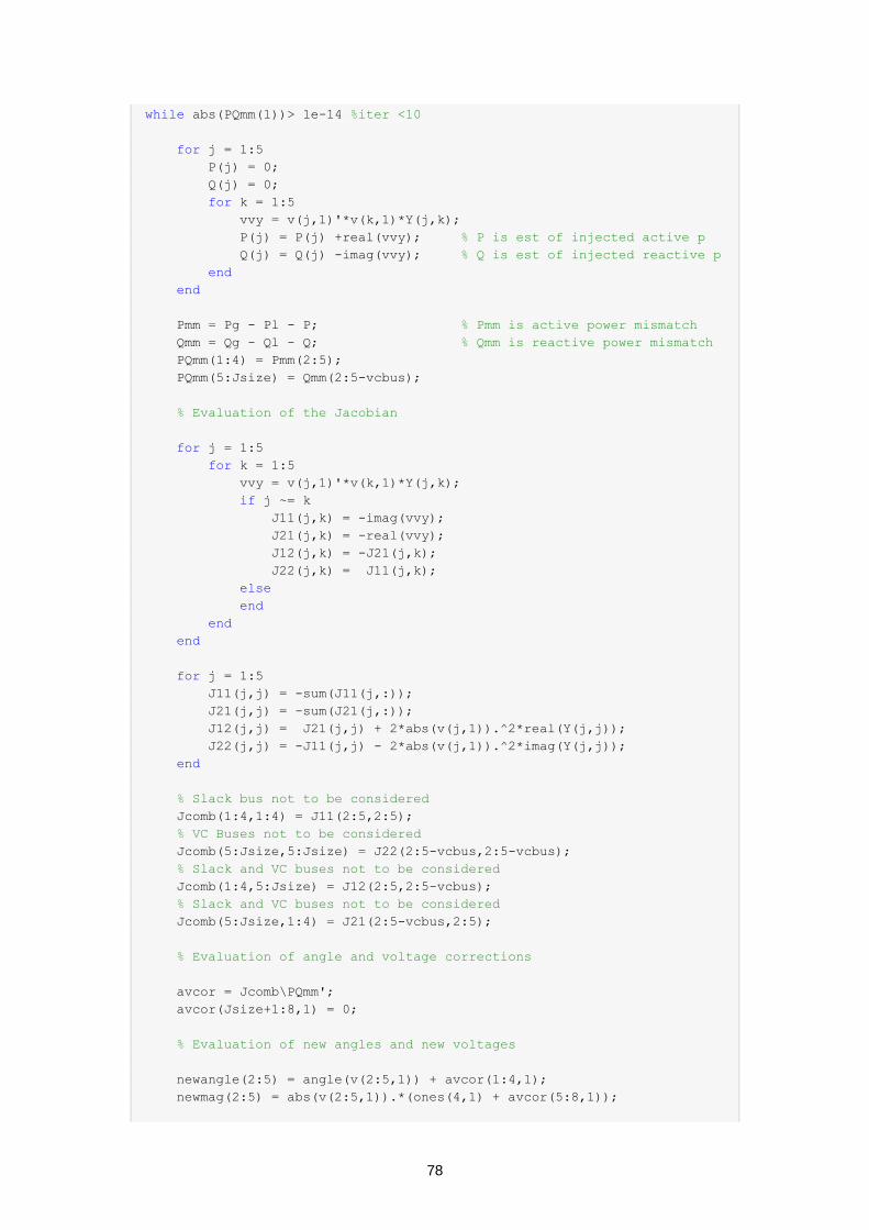
78
while abs(PQmm(1))> 1e-14 %iter <10
for j = 1:5
P(j) = 0;
Q(j) = 0;
for k = 1:5
vvy = v(j,1)'*v(k,1)*Y(j,k);
P(j) = P(j) +real(vvy); % P is est of injected active p
Q(j) = Q(j) -imag(vvy); % Q is est of injected reactive p
end
end
Pmm = Pg - Pl - P; % Pmm is active power mismatch
Qmm = Qg - Ql - Q; % Qmm is reactive power mismatch
PQmm(1:4) = Pmm(2:5);
PQmm(5:Jsize) = Qmm(2:5-vcbus);
% Evaluation of the Jacobian
for j = 1:5
for k = 1:5
vvy = v(j,1)'*v(k,1)*Y(j,k);
if j ~= k
J11(j,k) = -imag(vvy);
J21(j,k) = -real(vvy);
J12(j,k) = -J21(j,k);
J22(j,k) = J11(j,k);
else
end
end
end
for j = 1:5
J11(j,j) = -sum(J11(j,:));
J21(j,j) = -sum(J21(j,:));
J12(j,j) = J21(j,j) + 2*abs(v(j,1)).^2*real(Y(j,j));
J22(j,j) = -J11(j,j) - 2*abs(v(j,1)).^2*imag(Y(j,j));
end
% Slack bus not to be considered
Jcomb(1:4,1:4) = J11(2:5,2:5);
% VC Buses not to be considered
Jcomb(5:Jsize,5:Jsize) = J22(2:5-vcbus,2:5-vcbus);
% Slack and VC buses not to be considered
Jcomb(1:4,5:Jsize) = J12(2:5,2:5-vcbus);
% Slack and VC buses not to be considered
Jcomb(5:Jsize,1:4) = J21(2:5-vcbus,2:5);
% Evaluation of angle and voltage corrections
avcor = Jcomb\PQmm';
avcor(Jsize+1:8,1) = 0;
% Evaluation of new angles and new voltages
newangle(2:5) = angle(v(2:5,1)) + avcor(1:4,1);
newmag(2:5) = abs(v(2:5,1)).*(ones(4,1) + avcor(5:8,1));

79
for j = 2:5
v(j) = newmag(j)*exp(1i*newangle(j));
end
iter = iter+1;
end
% Calculate Power Factor at Buses
S = sqrt(P.^2 + Q.^2);
pf = abs(P)./S;
80
Appendix F - Hazard Assessment Check Forms
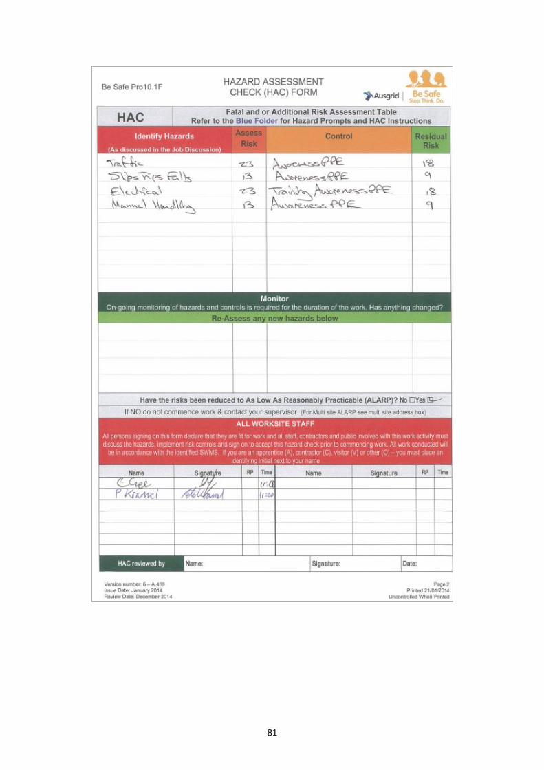
81
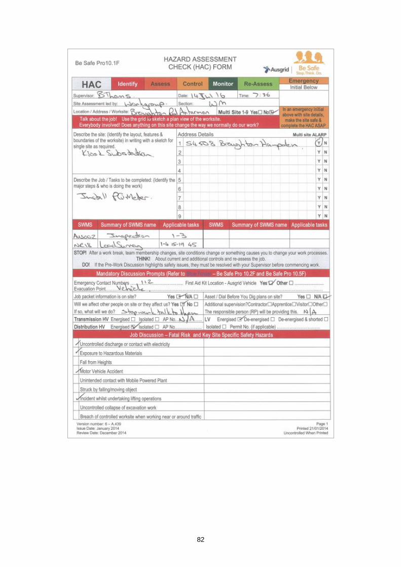
82
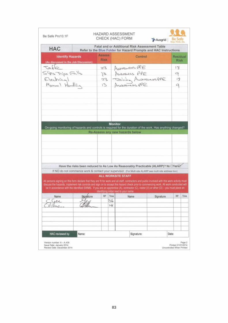
83
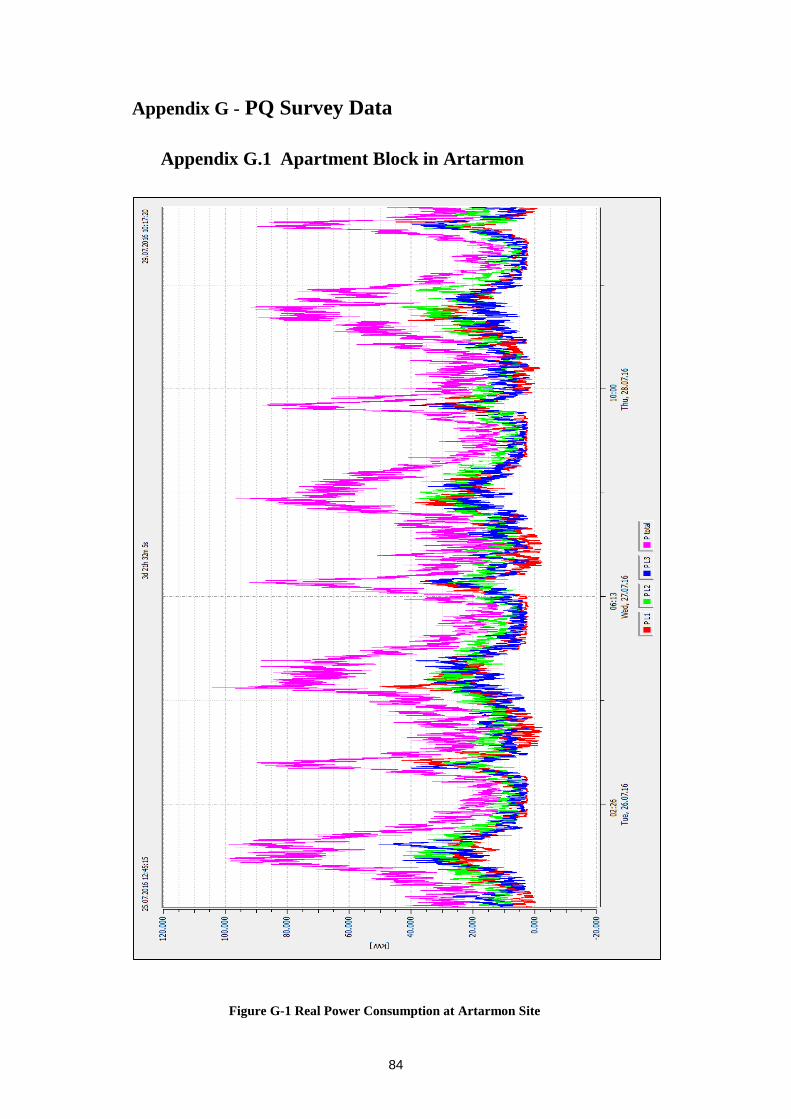
84
Appendix G - PQ Survey Data
Appendix G.1 Apartment Block in Artarmon
Figure G-1 Real Power Consumption at Artarmon Site
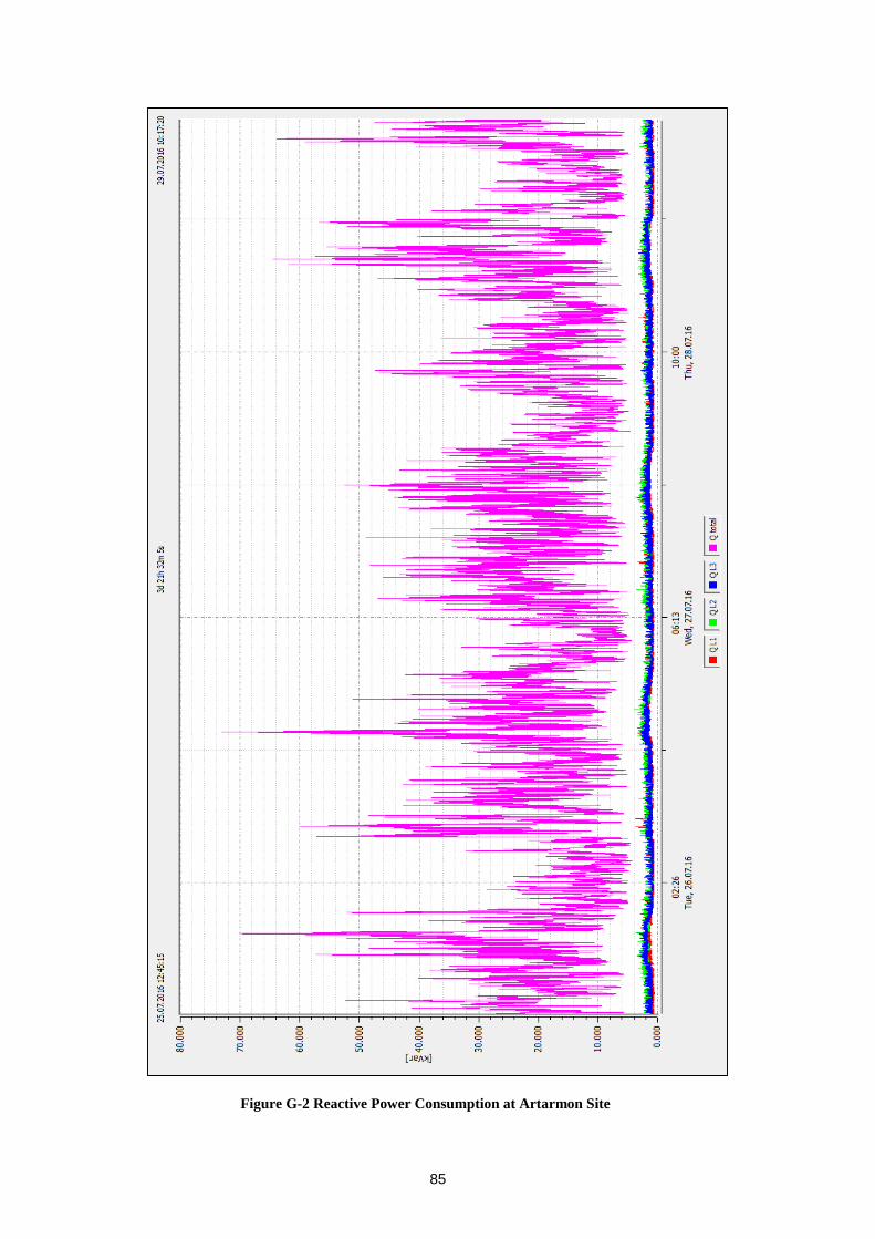
85
Figure G-2 Reactive Power Consumption at Artarmon Site
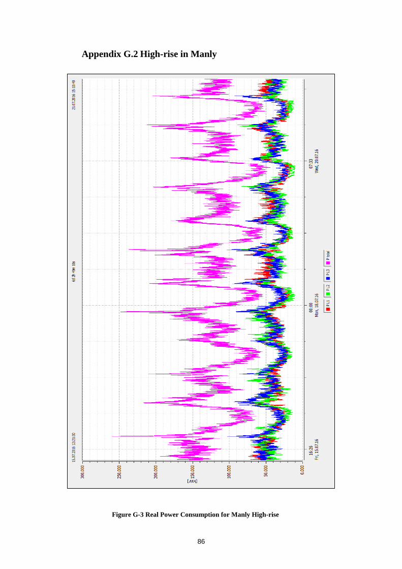
86
Appendix G.2 High-rise in Manly
Figure G-3 Real Power Consumption for Manly High-rise
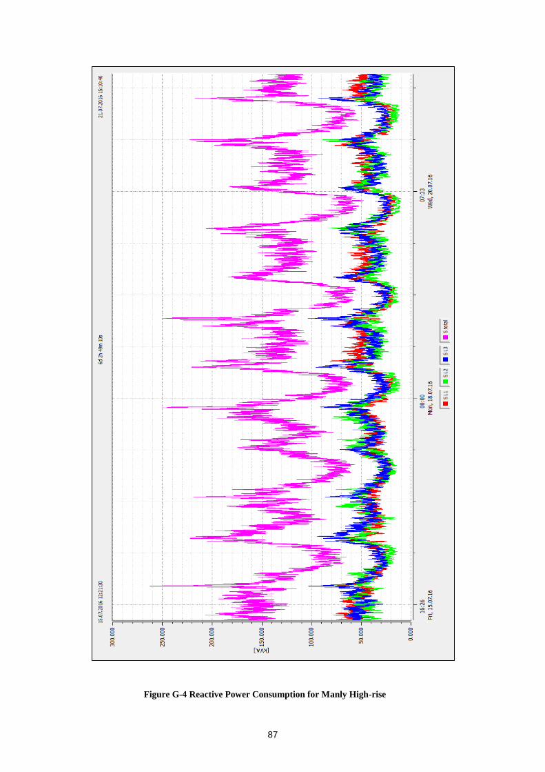
87
Figure G-4 Reactive Power Consumption for Manly High-rise

88
Appendix H - Literature Review
Introduction
The literature review for this project will focus on 4 main areas. The initial
investigation will focus on Distributed generation, mainly from renewable energies.
Secondly, the impact reactive power has on the power factor and supply voltage of
individual premises. Thirdly, the use of SMART meters in Australia and what
information is capable of being read from a SMART meter in real time. Lastly a
comprehensive review of STATCOM’s and their ability to supply and absorb
reactive power. Conducting this research will provide sound knowledge which will
be needed during the laboratory testing early on in the project. The aim of the testing
will be to see if the STATCOM is able to vary the amount of reactive power
depending on the power factor of the installation which is being read from the
SMART meter.
Distributed Generation
The use of renewable energy sources for the generation of electricity is seen as one
of the important ways of reducing carbon dioxide emissions(Abu-Sharkh et al.
2006). This distributed generation is also known as embedded generation, the most
common form of this embedded generation in Australia is the installation of PV
arrays and these tend to be small scale. These systems generate power from the
sunlight during the day and lay dormant during the night time, often when domestic
load requirements are at their peak.
Benefits of Embedded Generation
The customer who has installed the embedded generation will be the one who sees
the most benefit of the embedded generation as would be expected. If they are savvy
with their electrical load they can ensure that the majority of the power that they are
generating is consumed by necessary electrical equipment in their household during
the day, such as a washing machine, dishwasher or scheduling a pool pump for

89
more hours of operating during the day. This ensures that the electricity they use
will be from their generation and not supplied form the grid at an extra cost to them.
There are also the Environmental benefits to be gained from local embedded
generation. Using the solar energy from the sun produces no carbon emissions as
appose to obtaining that energy from the grid which is most likely generating energy
from burning coal and producing large amounts of greenhouse gas emissions.
Disadvantages of Embedded Generation
Embedded generation can have adverse effects on the distribution authority’s
electricity grid, some of these effects include an increase in fault levels, potential
reverse power flow problems during blackouts, and increases in steady state voltage
levels.
Bhattacharya (Bhattacharya, Saha & Hossain 2013) states that even though the fault
current contribution from individual PV systems installed on residences is not high,
collective contribution from multiple PV systems connected across the network can
make a significant increase in fault current. The electricity network will need to
monitor the amount of penetration of embedded generation in local areas to ensure
that the increase in fault level is manageable.
Power previously has flowed from the large scale generators through the
transmission network, to the distribution network to the end customer. Having a
higher penetration of embedded generation is changing this traditional linear flow
into a bi directional flow. Also cause for concern is if multiple embedded systems
are only connected to one phase from a TX this will create a large unbalanced power
flow and will increase return current in the neutral conductors.
Reactive Power
Reactive power and voltage control is one of the ancillary services used to maintain
the voltage profile through injecting or absorbing reactive power (Dapu et al. 2005).

90
Reactive power plays an important role in the voltage control of an electrical
system. An electrical system supplies two types of power, real power or true power,
which is the actual amount of power being used to do useful work and is measured
in watts (W). The other power is reactive power and is measured in Volt-Amps-
Reactive (VAR). If the voltage on a system is too low it will not be able to supply
active power, thus reactive power is required to provide the voltage levels needed
on the system.
Zhao states reactive power is location dependent, and long distance transfer is not
wanted (Dapu et al. 2005). For this reason, it is best that the reactive power be
produced as close to the load as possible, this will also save on transmission losses
associated with the reactive power.
Voltage Control
On an AC system voltage control is managed by absorbing and producing reactive
power. Managing reactive power in this way in affect changes the phase shift
between the current and the supply voltage, producing reactive power will have a
capacitive effect and will cause a leading power factor, whereas absorbing reactive
power will have an inductive effect and cause a lagging power factor. Tanaka
(Tanaka et al. 2009) states that reactive power control has a possibility to contribute
for reduction of distribution loss.
In 2011 the Australian Standards PQ Committee published AS 61000.3.100-2011
(Standards 2011), this defines that the voltage at a premises needs to be within the
rage of 230 V +10% or -6%. The further away from a TX a supply is generally
means the lower their supply voltage will be. This problem is worsened during
periods of high load, which for residential loads tends to be in the early evening.
SMART Meters
Many electricity distributors around Australia have begun the roll out of SMART
meters to its residential customers. These smart meters are able to supply far more

91
information than the previously installed disc meters which only gave a reading of
how much energy had been used. Capua (De Capua et al. 2014) states that in recent
years there has been a significant growth in the diffusion of renewable energy
systems. This increase in renewable energies at the local load will call for a
substantial change being required from the electricity distributors. They will be
required to gradually change from a ‘passive’ network, in which electricity flows
only from the place of production to the point of consumption, to an ‘active’ and
‘smart’ network, that is Smart Grid, which is able to manage and regulate electrical
flow traveling in a discontinuous and bidirectional way (Molderink et al. 2010).
Communication with the SMART meter is a variety of ways, the three most
common ways that have been reviewed by Ali (Ali, Maroof & Hanif 2010) are:
RS-232 As Local transmission medium
PLCC Using main power line
Short Messaging Service on GSM
Ali acknowledges that the PLCC medium is the more efficient and preferable
medium of transmission, Power line communication or Power line networking
(PLN) which utilises the same wired medium through which power is delivered to
the customer as a communication channel (Ali, Maroof & Hanif 2010). Using
PLCC as a medium means there would not be any further wiring required for the
communication.
STATCOM
STATCOM, as an advanced compensator, consists of a Voltage Source Inverter
(VSI) which is connected through shunt TX to the network (Toodeji, Farokhnia &
Riahy 2009). They are commonly used and installed onto electricity networks to
improve power factor and decrease the effects of poor VR. A DC voltage source is
converted into an AC waveform using a STATCOM. Alone the STATCOM has
very little active power capability due to the voltage source coming from a DC
capacitor, but this can be improved if use in conjunction with a suitable energy

92
storage device such as a battery. Han (Junbiao et al. 2012) has studied and shown
that in a weak system with PV generation, STATCOM has an excellent scope for
mitigating most of the PQ issues such as harmonics, voltage flicker, and transient
voltage.