JANI HONKANEN

HARMONIC PERFORMANCE IMPROVEMENT OF STATCOM

Master of Science Thesis

Examiners: Assist. Prof. Tuomas Messo and Ph.D. Jenni Rekola Examiners and topic approved on 28th February 2018

i

ABSTRACT

JANI HONKANEN: Harmonic Performance Improvement of STATCOM Tampere University of Technology Master of Science Thesis, 82 pages, 3 Appendix pages April 2018 Master’s Degree Programme in Electrical Engineering Major: Power Electronics Examiners: Assistant Professor Tuomas Messo and Ph.D. Jenni Rekola Keywords: STATCOM, harmonic currents, harmonic voltages, reactive power compensation

In this thesis, harmonic performance of STATCOM (Static Synchronous Compensator)

was studied. Harmonic performance means the amount of harmonic current emissions

and their effect on harmonic voltages at the connection point of the compensator. It has

been observed that harmonic current emissions are small when grid voltage is sinusoidal

but they increase when harmonics are added to grid voltage. This is a problem as the

currents cause harmonic voltages in grid impedances which are added to the existing grid

harmonic voltages at the connection point. Standards and transmission operators’ speci-

fications set limits for harmonic voltages at the connection point which are exceeded in

some cases with the present current emissions.

The objective of the thesis was to study reasons for the problem and decrease harmonic

current emissions. The problem was studied by simulations in PSCAD. Harmonic current

and voltage spectrums at the connection point of STATCOM were simulated with same

grid harmonic voltages in several cases where some STATCOM attributes were modified.

Especially, the effect of different control functions on harmonic performance was studied.

Two voltage feedforward options were compared. It was observed that harmonic currents

of orders from 20 to 40 were smaller with fundamental component feedforward. Instan-

taneous value of voltage as feedforward is intended to remove harmonic currents com-

pletely. It was noticed that the delay caused by modulator deteriorates its performance

especially at high-order harmonics. Low-order harmonics were still smaller than with

fundamental feedforward. However, the performance of a real system will not be so good

due to errors in harmonic voltage measurement. Also, performance with low-pass filtered

feedforward was investigated. Harmonic currents around 30th were well mitigated. Low-

order harmonics were smaller than with fundamental feedforward but not as small as with

instantaneous feedforward due to filter’s phase delay.

Low-order harmonic currents were reduced to almost zero by actively controlling them.

Control was implemented by adding resonant branches for these harmonics in PR-con-

troller (proportional-resonant controller). Second harmonic current could be removed

only partly by control. Part of it resulted from the controller which controls the average

of DC-voltages in STATCOM branches to nominal value. Still, harmonic current control

requires exact harmonic current measurement which may be challenging in a real system.

Second harmonic current was observed to increase in voltage control mode when operat-

ing point was shifted from capacitive to inductive. To mitigate it, a band-stop filter was

designed for voltage d-component which is produced by synchronization.

ii

TIIVISTELMÄ

JANI HONKANEN: STATCOM:n harmonisen suorituskyvyn parantaminen Tampereen teknillinen yliopisto Diplomityö, 82 sivua, 3 liitesivua Huhtikuu 2018 Sähkötekniikan diplomi-insinöörin tutkinto-ohjelma Pääaine: Tehoelektroniikka Tarkastajat: Apulaisprofessori Tuomas Messo ja tutkijatohtori Jenni Rekola Avainsanat: STATCOM, harmoniset virrat, harmoniset jännitteet, loistehon kom-pensointi

Tässä diplomityössä tutkittiin STATCOM:n harmonista suorituskykyä. Sillä tarkoitetaan

tuotettujen harmonisten virtojen määrää ja niiden vaikutusta laitteen liityntäpisteen har-

monisiin jännitteisiin. On havaittu, että harmoniset virrat ovat pieniä verkon jännitteen

ollessa sinimuotoista. Ne kuitenkin kasvavat, kun jännitteeseen lisätään harmonisia kom-

ponentteja. Kasvu on ongelma, sillä virrat aiheuttavat harmonisia jännitteitä verkkoimpe-

dansseissa, jotka lisätään liityntäpisteessä verkon harmonisiin jännitteisiin. Liityntäpis-

teen harmonisten jännitteiden määrälle asetetaan rajoituksia standardeissa ja verkkoyhti-

öiden spesifikaatioissa, jotka ylittyvät nykyisillä virroilla joissain tapauksissa.

Työn tavoitteena oli tutkia ongelman syitä ja pienentää tuotettuja harmonisia virtoja. On-

gelmaa tutkittiin tekemällä simulaatioita PSCAD:lla. Niissä tutkittiin harmonisten virto-

jen ja jännitteiden määrää STATCOM:n liityntäpisteessä, kun verkon harmoniset jännit-

teet pidettiin samana ja joitain STATCOM:n ominaisuuksia muutettiin. Erityisesti tutkit-

tiin säätöominaisuuksien vaikutusta harmoniseen suorituskykyyn.

Simuloinneissa vertailtiin kahta eri jännitettä myötäkytkentänä. Havaittiin, että perustaa-

juista jännitettä käytettäessä harmoniset virrat järjestykseltään 20:stä 40:een olivat pie-

nempiä. Hetkellisen jännitteen käyttämisen tarkoitus on poistaa harmoniset virrat täysin,

mutta sen suorituskyvyn havaittiin huononevan modulaattorin aiheuttaman viiveen

vuoksi etenkin suurilla taajuuksilla. Pienitaajuiset harmoniset virrat olivat kuitenkin pie-

nempiä kuin perustaajuisella myötäkytkennällä. Todellisen järjestelmän suorituskyky ei

kuitenkaan ole yhtä hyvä johtuen virheistä harmonisten jännitteiden mittauksessa. Myös

alipäästösuodatetun myötäkytkennän suorituskykyä tutkittiin. Virrat 30:n harmonisen

ympäristössä olivat hyvin vaimentuneita. Matalataajuiset harmoniset olivat pienempiä

kuin perustaajuista jännitettä käytettäessä, mutta ei yhtä pieniä kuin hetkellistä jännitettä

käytettäessä suodattimen aiheuttaman viiveen takia.

Matalataajuiset harmoniset virrat saatiin vähennettyä melkein nollaan niitä säätämällä.

Säätö toteutettiin lisäämällä PR-säätimeen resonanssihaaroja näille harmonisille kom-

ponenteille. Toinen harmoninen pystyttiin poistamaan säädön avulla vain osittain. Osan

siitä havaittiin johtuvan säätimestä, joka säätää STATCOM:n haarojen DC-jännitteiden

keskiarvon nimelliseen arvoonsa. Säätö vaatii kuitenkin toimiakseen tarkan harmonisten

virtojen mittauksen, mikä voi olla todellisessa järjestelmässä haastavaa.

Toisen harmonisen virran havaittiin kasvavan jännitesäätömoodissa, kun toimintapiste

siirtyi kapasitiivisesta induktiivista kohti. Virran vaimentamiseksi suunniteltiin kaistanes-

tosuodin synkronisaation tuottamalle jännitteen d-komponentille.

iii

PREFACE

This Master of Science Thesis was written for GE Grid Solutions Oy between September

2017 and April 2018. Thesis project has been an interesting experience from which I have

learned a lot.

I have many people to thank for their contribution to the thesis. My instructor Ph.D. Anssi

Mäkinen within the company offered me very good guidance and comments which im-

proved the quality of the work considerably. MSc. Sami Kuusinen assisted me especially

in PSCAD simulations and commented the work at its early stage. Joni Toppari was writ-

ing his thesis simultaneously within the company of a subject related closely to my thesis.

Sharing thoughts with him gave me many ideas to improve the work.

I would like to thank Assistant Professor Tuomas Messo and Ph.D. Jenni Rekola for ex-

amining my thesis. I also would like to thank my supervisor MSc. Vesa Oinonen for of-

fering me this position and organizing the thesis process. In addition, I would like to thank

my colleagues for sharing their knowledge with me. Finally, I am especially grateful to

my family and girlfriend for their support during my studies and thesis project.

Tampere, 11.4.2018

Jani Honkanen

iv

CONTENTS

1. INTRODUCTION .................................................................................................... 1

2. HARMONICS ........................................................................................................... 2

2.1 Harmonic currents and voltages ..................................................................... 2

2.2 Effects of harmonics....................................................................................... 4

2.3 Resonances ..................................................................................................... 5

2.4 Harmonic indexes ........................................................................................... 7

2.5 Harmonic emission standards ........................................................................ 8

3. REACTIVE POWER COMPENSATION .............................................................. 11

3.1 Reactive power ............................................................................................. 11

3.2 Passive shunt compensators ......................................................................... 12

3.3 Passive series compensators ......................................................................... 17

3.4 SVC .............................................................................................................. 18

3.5 STATCOM ................................................................................................... 20

3.5.1 Operating principle ........................................................................ 21

3.5.2 Modular Multilevel Converter ....................................................... 22

3.5.3 Control system ............................................................................... 24

4. HARMONIC CURRENTS AND VOLTAGES OF STATCOM ........................... 28

4.1 Harmonic current emissions with sinusoidal grid voltage ........................... 28

4.2 Harmonic current emissions with distorted grid voltage ............................. 31

4.3 Effect of harmonic currents on PCC voltage in inductive grid .................... 35

4.4 Effect of harmonic currents on PCC voltage in capacitive grid ................... 41

4.5 Comparison of voltage feedforward options ................................................ 47

4.6 Harmonic current emissions with filtered voltage feedforward ................... 49

4.7 Harmonic current emissions with increased reactance ................................ 51

5. SOURCES OF HARMONIC CURRENTS ............................................................ 54

5.1 Modulator effect ........................................................................................... 54

5.2 Current control effect ................................................................................... 58

5.3 DC-link voltage control effect...................................................................... 65

5.4 Voltage control effect ................................................................................... 68

6. FUTURE WORK .................................................................................................... 80

7. CONCLUSIONS ..................................................................................................... 81

REFERENCES ................................................................................................................ 83

APPENDIX A: CONTROL BLOCK DIAGRAM

APPENDIX B: SIMULATION PARAMETERS

v

LIST OF SYMBOLS AND ABBREVIATIONS

AC Alternating Current

DC Direct Current

GTO Gate-Turn-Off

IGBT Insulated Gate Bipolar Transistor

IGCT Integrated Gate Commutated Thyristor

LPF Low-Pass Filter

MMC Modular Multilevel Converter

PCC Point of Common Coupling

PI Proportional-integral

PR Proportional-resonant

p.u Per unit

PWM Pulse Width Modulation

RMS Root-Mean-Square

STATCOM Static Synchronous Compensator

SVC Static Var Compensator

TCR Thyristor Controlled Reactor

TDD Total Demand Distortion

THD Total Harmonic Distortion

THDI Total Harmonic Distortion for Current

THDV Total Harmonic Distortion for Voltage

TSC Thyristor Switched Capacitor

C Capacitance

E Voltage magnitude produced by STATCOM

f1 Fundamental frequency

fres Resonance frequency

Gh Transfer function of a harmonic resonant branch

Gh,ideal Transfer function of the sum of ideal harmonic resonant branches

Gh,non-ideal Transfer function of the sum of non-ideal harmonic resonant

branches

GPR,ideal Transfer function of ideal PR-controller

GPR,non-ideal Transfer function of non-ideal PR-controller

h Harmonic component order

hmax Maximum harmonic order used in TDD and THD calculations

i Instantaneous value of current

i Current vector

I RMS value of current

I1 RMS value of fundamental current

icap Instantaneous value of capacitor current

IC RMS value of capacitor current

id Current d-component

id,ab,ref Current d-component reference in stationary frame

id,ref Current d-component reference

IDC Current DC-component

Ih RMS current of harmonic component h

Ih,PCC RMS current of harmonic component h at PCC

𝐼h,STATCOM Harmonic current produced by STATCOM

iL Instantaneous value of inductor current

vi

IL Total demand current

IP Current active component

iq Current q-component

iq,ab,ref Current q-component reference in stationary frame

iq,ref Current q-component reference

IQ Current reactive component

IresC Capacitor current at the resonance frequency

IresL Inductor or grid current at the resonance frequency

ISC Short-circuit current

j Imaginary operator

k Discrete time instant

KI Integral gain

KIh Integral gain at harmonic order h

KP Proportional gain

L Inductance

n Number of series-connected submodules in one phase

p Instantaneous active power

P Active power

q Instantaneous reactive power

Q Reactive power

QC Capacitive reactive power

Qf Quality factor of the resonance circuit

R Resistance

s Laplace transform variable

S Apparent power

t Time

Ts Sampling period

uh Resonant controller input for one harmonic

v Instantaneous value of voltage

v Voltage vector

V RMS value of voltage

v0 Zero sequence voltage

V1 RMS value of fundamental voltage

va Instantaneous value of a-phase voltage

vb Instantaneous value of b-phase voltage

vc Instantaneous value of c-phase voltage

vcap Instantaneous value of capacitor voltage

Vcs Resonance frequency voltage at the harmonic source terminals

vd Voltage d-component

VDC DC-voltage in a submodule capacitor

vdq Voltage vector in synchronous frame

Vh RMS voltage of harmonic component h

Vhi Harmonic voltage component h caused by source i

𝑉h,grid Harmonic voltage in grid

𝑉h,PCC Harmonic voltage at PCC

Vh,PCC RMS voltage of harmonic component h at PCC

Vh,total Statistical total harmonic voltage from several sources

vL Instantaneous value of inductor voltage

Vn1 Voltage magnitude at node 1

Vn2 Voltage magnitude at node 2

vii

Vp Connection point voltage at the parallel resonance frequency

Vpcc PCC voltage

vq Voltage q-component

Vs Connection point voltage at the series resonance frequency

vα Voltage α-component

vαβ Voltage vector in αβ-frame

vβ Voltage β-component

X Reactance

XC Capacitive reactance

Xh,grid Grid reactance at harmonic order h

XL Inductive reactance

Xsource Transmission line reactance

XT Transformer reactance

yh Resonant controller output for one harmonic

z Z-transform variable

�̅� Complex impedance

Zgrid Grid impedance magnitude

𝑍h,grid Grid impedance at harmonic order h

Zh,STATCOM STATCOM impedance magnitude at harmonic order h

Zp Parallel impedance at the resonance frequency

α α-axis

β β-axis

γ Exponent used in summing harmonic voltages from different sources

δ Angle difference between voltages

δu Imaginary part of voltage drop

Δu Real part of voltage drop

θ Transformation angle in αβ- to dq -transformation

𝜄 ̅ Current phasor

�̅�1 Phasor of voltage at node 1

�̅�2 Phasor of voltage at node 2

φ Angle difference between voltage and load current

φh Angle of the harmonic component h

φI Current angle

φI,h,PCC Current angle at harmonic order h at PCC

φV Voltage angle

φV,h,PCC Voltage angle at harmonic order h at PCC

φZ,h,STATCOM STATCOM impedance angle at harmonic order h

ω Angular frequency

ω1 Fundamental angular frequency

ωc Cut-off angular frequency

ωpw Pre-warp angular frequency

ωres Resonance angular frequency

1

1. INTRODUCTION

The increasing use of power electronic converters has caused the amount of harmonic

currents and voltages to increase in power systems [1]. Harmonics cause harmful effects

on power system components and some devices connected in the grid such as power

losses and heating. Thus, their amount is limited by standards and transmission system

operators’ specifications. Usually, harmonic voltages at the connection point of a cus-

tomer or a device are limited.

At the same time, the demand for electricity is growing in many areas. Many loads like

electric motors need inductive reactive power which reserves transmission capacity from

the active power. To maximize the active power transmission capacity of the grid and

support grid voltage, reactive power is compensated. One modern solution for reactive

power compensation is STATCOM (Static Synchronous Compensator) which consists of

a step-down transformer, a reactor and a voltage-source converter [2].

Harmonic performance of a STATCOM system is studied in this thesis. Harmonic current

emissions of studied STATCOM are small if grid voltage is sinusoidal but the problem is

that they increase as harmonic voltages in grid increase. The purpose of this thesis is to

study reasons for the problem and the effect of increased harmonic currents on harmonic

voltages at the connection point. Another objective is to find solutions to decrease har-

monic current emissions so that standard and specification requirements would be met.

Harmonic performance is studied by simulations using a PSCAD-model which is intro-

duced later in the thesis.

In chapter 2, harmonics, their effects and standards that limit them are introduced. In

chapter 3, common reactive power compensation systems are described. Especially, the

structure of studied STATCOM and its control system are explained. In chapter 4, the

phenomenon of increasing STATCOM’s harmonic current emissions due to increasing

grid harmonic voltages is shown. Harmonic emissions are compared with two considered

voltage feedforward options. Moreover, effect of harmonic currents on harmonic voltages

at the connection point of STATCOM and the reduction of harmonic currents by increas-

ing the impedance of passive components are studied.

In chapter 5, the impacts of modulator and different control functions on harmonic current

emissions are investigated. Solutions to improve these functions in the viewpoint of har-

monics are developed or suggested. In chapter 6, future work to improve harmonic per-

formance further is suggested. Finally, conclusions are given in chapter 7.

2

2. HARMONICS

Harmonic currents and voltages cause adverse effects in power systems. They are pro-

duced by nonlinear loads in the network. The growing use of power electronics increases

harmonic voltage and current levels in the grid. That is why harmonic emission limits for

equipment are set by standards.

In this chapter, harmonics and their harmful effects are described. Also, resonances are

described which amplify the existing harmonic levels. Total amount of harmonics can be

expressed as indexes which are introduced. Moreover, standards which limit the amount

of harmonics are introduced.

2.1 Harmonic currents and voltages

In ideal network currents and voltages are sinusoidal typically at 50 or 60 Hz frequency.

In real network, they are usually periodical but distorted which means that they differ

from ideal sinusoidal shape. Mathematician Joseph Fourier figured that this kind of signal

can be presented as a sum of a constant signal, a sinusoid at fundamental frequency and

sinusoids whose frequencies are fundamental frequency multiplied by an integer. These

integer multiplied frequencies are called harmonic frequencies. So, current signal i(t) can

be presented as Fourier series:

𝑖(𝑡) = 𝐼DC + ∑ √2𝐼hsin(2𝜋ℎ𝑓1𝑡 + 𝜑h)∞h=1 , (1.1)

where IDC is current DC-component, Ih is the RMS (Root-Mean-Square) value of the har-

monic component h current, f1 is fundamental frequency (typically 50 or 60 Hz), t is time

and φh is the angle of harmonic component h [3].

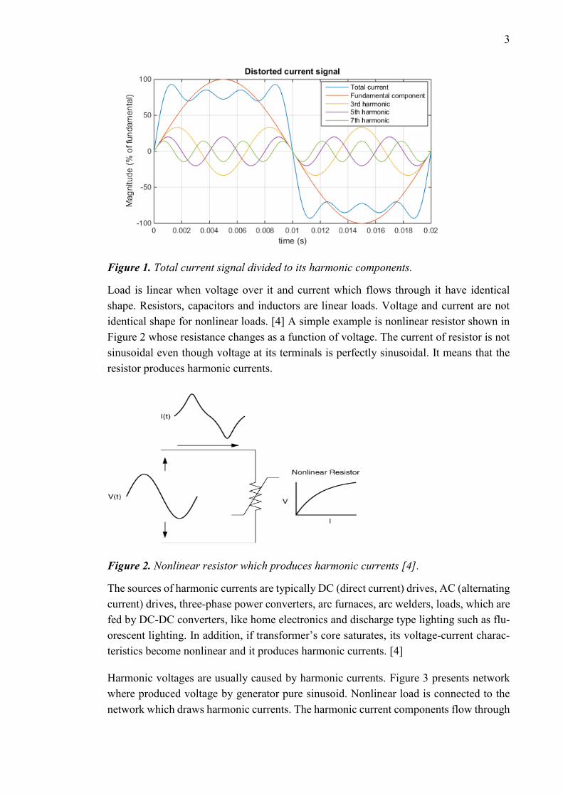
Figure 1 presents a distorted current signal which consists of fundamental frequency as

well as 3rd, 5th and 7th harmonic components. It is typical that even harmonics are small

in electric networks because most devices behave equally positive and negative polarity.

Signal does not contain even harmonics when it is symmetrical with respect to time axis.

One exception is half-wave rectifier which draws current only one polarity. [4]

3

Figure 1. Total current signal divided to its harmonic components.

Load is linear when voltage over it and current which flows through it have identical

shape. Resistors, capacitors and inductors are linear loads. Voltage and current are not

identical shape for nonlinear loads. [4] A simple example is nonlinear resistor shown in

Figure 2 whose resistance changes as a function of voltage. The current of resistor is not

sinusoidal even though voltage at its terminals is perfectly sinusoidal. It means that the

resistor produces harmonic currents.

Figure 2. Nonlinear resistor which produces harmonic currents [4].

The sources of harmonic currents are typically DC (direct current) drives, AC (alternating

current) drives, three-phase power converters, arc furnaces, arc welders, loads, which are

fed by DC-DC converters, like home electronics and discharge type lighting such as flu-

orescent lighting. In addition, if transformer’s core saturates, its voltage-current charac-

teristics become nonlinear and it produces harmonic currents. [4]

Harmonic voltages are usually caused by harmonic currents. Figure 3 presents network

where produced voltage by generator pure sinusoid. Nonlinear load is connected to the

network which draws harmonic currents. The harmonic current components flow through

4

the network impedances causing voltage drop at each harmonic component. The voltage

at the connection point of the load is the original sinusoidal voltage minus the voltage

drop. Thus, also the voltage at the connection point contains harmonic components.

Figure 3. The principle of harmonic voltage generation [4].

2.2 Effects of harmonics

Harmonic currents and voltages cause many unfavorable effects. Because harmonic cur-

rents are additional currents flowing through grid conductors and transformers they cause

power losses. Moreover, harmonic voltages cause additional losses due to eddy currents

and hysteresis in transformer core [5]. Also, conductor resistance increases as a function

of frequency because of skin and proximity effects [6]. Increased resistance means even

more losses.

The additional losses in the network components cause them to heat. The increase of

temperature can shorten cable and transformer lifetimes [7, 8]. Also, if voltage peak value

increases because of the harmonic voltages, more dielectric stress is caused to the cable

and transformer insulators. Increased dielectric stress shortens insulator lifetime [9]. If

the system is desired to have a certain lifetime, voltage ratings of the components must

be chosen larger than without harmonics.

Harmonic voltages at the connection point of electric motor cause harmonic magnetizing

currents in stator and thus harmonic magnetic fluxes in the iron core and rotor [4]. These

harmonic fluxes induce eddy currents to the core and harmonic currents to the rotor. Thus,

power losses of the motor increase. Some harmonic components are positive sequence

which means 120-degree phase shift between phases in normal A-B-C rotation order [4].

Some of them are negative sequence which means same phase shift between phases but

in order A-C-B [4]. Positive sequence currents cause torques to same direction and neg-

ative sequence currents to another direction than the positive sequence fundamental com-

ponent [9]. The torque components introduced by harmonics make the total torque pul-

sating. Pulsating torque causes mechanical stress to the motor and increased vibration

[10]. Increased vibration causes higher audible noise in motors [11]. Harmonic currents

also increase vibrations and noise in transformers [12].

5

Especially harmonics whose orders are odd multiples of the third harmonic (3, 9, 15, 21,

…) are harmful if they are not considered in the planning of the system. If current is

balanced in three phases, these triplen harmonic currents are in the same phase in all phase

conductors and they add in the wye point to the neutral conductor. In balanced condition,

three times higher current at the triplen harmonic frequency flows in neutral conductor

compared to the phase conductors. That may cause neutral conductor overloading and

telephone interference. These harmonics in different phase conductors which have equal

magnitude and are in phase with each other are called zero sequence harmonics. [4]

The flow of the balanced triplen harmonics, or more generally zero sequence currents,

from transformer primary to secondary or vice versa can be blocked by appropriate trans-

former connections. In Figure 4 is presented the flow of the balanced triplen harmonic

currents in wye-delta connection.

Figure 4. The flow of balanced triplen harmonic currents in wye-delta transformer [4].

The triplen harmonics are induced in the secondary but as they are in phase and equal

magnitude they flow only in the delta and do not appear in secondary line currents. How-

ever, this applies only if currents are balanced in three phases. If triplen harmonic currents

are unbalanced, only part of them are zero sequence. Rest of them are positive and/or

negative sequence which can flow to the secondary phase conductors also. [4]

Moreover, harmonic currents can cause errors in older electric energy meters [4] or in

operation of older electronic relays whose protection limits are based on current peak

value [13]. They can also cause interference to electronic appliances and communication

networks [1].

2.3 Resonances

Shunt capacitor banks are used to compensate reactive power in the network which is

explained in detail later. However, they may cause parallel or series resonances which

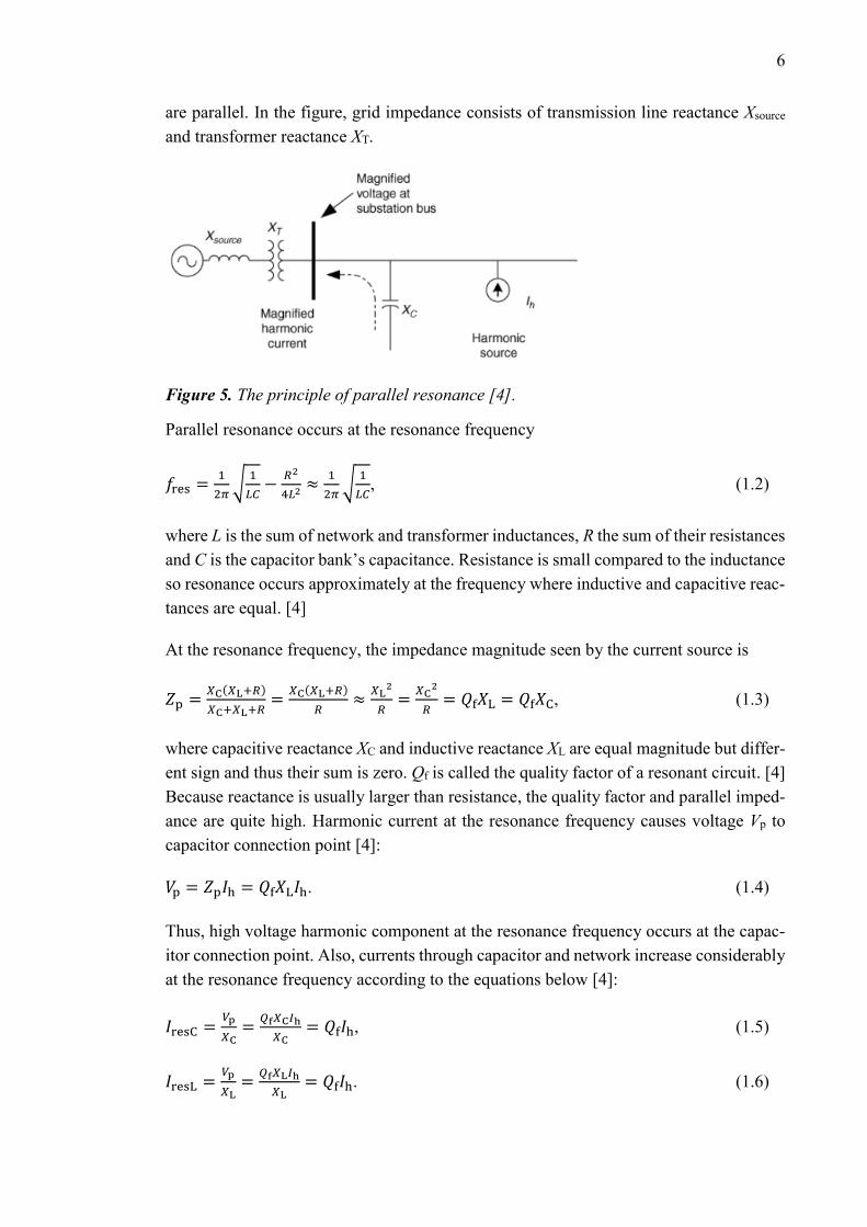
amplify existing harmonic currents and voltages. Figure 5 presents the principle of how

parallel resonance is composed. There is a current source which emits harmonic currents.

From its viewpoint inductive grid impedance and capacitor bank’s capacitive impedance

6

are parallel. In the figure, grid impedance consists of transmission line reactance Xsource

and transformer reactance XT.

Figure 5. The principle of parallel resonance [4].

Parallel resonance occurs at the resonance frequency

𝑓res =1

2𝜋√

1

𝐿𝐶−

𝑅2

4𝐿2 ≈1

2𝜋√

1

𝐿𝐶, (1.2)

where L is the sum of network and transformer inductances, R the sum of their resistances

and C is the capacitor bank’s capacitance. Resistance is small compared to the inductance

so resonance occurs approximately at the frequency where inductive and capacitive reac-

tances are equal. [4]

At the resonance frequency, the impedance magnitude seen by the current source is

𝑍p =𝑋C(𝑋L+𝑅)

𝑋C+𝑋L+𝑅=

𝑋C(𝑋L+𝑅)

𝑅≈

𝑋L2

𝑅=

𝑋C2

𝑅= 𝑄f𝑋L = 𝑄f𝑋C, (1.3)

where capacitive reactance XC and inductive reactance XL are equal magnitude but differ-

ent sign and thus their sum is zero. Qf is called the quality factor of a resonant circuit. [4]

Because reactance is usually larger than resistance, the quality factor and parallel imped-

ance are quite high. Harmonic current at the resonance frequency causes voltage Vp to

capacitor connection point [4]:

𝑉p = 𝑍p𝐼h = 𝑄f𝑋L𝐼h. (1.4)

Thus, high voltage harmonic component at the resonance frequency occurs at the capac-

itor connection point. Also, currents through capacitor and network increase considerably

at the resonance frequency according to the equations below [4]:

𝐼resC =𝑉p

𝑋C=

𝑄f𝑋C𝐼h

𝑋C= 𝑄f𝐼h, (1.5)

𝐼resL =𝑉p

𝑋L=

𝑄f𝑋L𝐼h

𝑋L= 𝑄f𝐼h. (1.6)

7

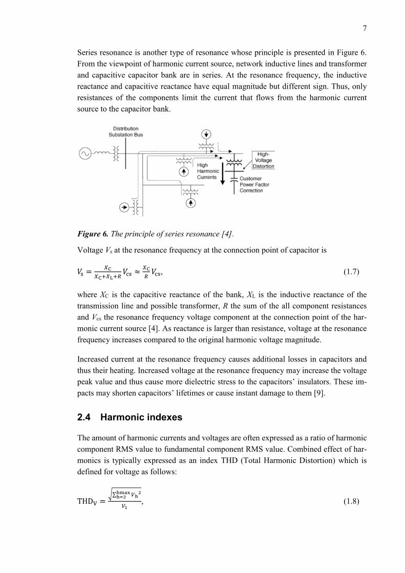
Series resonance is another type of resonance whose principle is presented in Figure 6.

From the viewpoint of harmonic current source, network inductive lines and transformer

and capacitive capacitor bank are in series. At the resonance frequency, the inductive

reactance and capacitive reactance have equal magnitude but different sign. Thus, only

resistances of the components limit the current that flows from the harmonic current

source to the capacitor bank.

Figure 6. The principle of series resonance [4].

Voltage Vs at the resonance frequency at the connection point of capacitor is

𝑉s =𝑋C

𝑋C+𝑋L+𝑅𝑉cs ≈

𝑋C

𝑅𝑉cs, (1.7)

where XC is the capacitive reactance of the bank, XL is the inductive reactance of the

transmission line and possible transformer, R the sum of the all component resistances

and Vcs the resonance frequency voltage component at the connection point of the har-

monic current source [4]. As reactance is larger than resistance, voltage at the resonance

frequency increases compared to the original harmonic voltage magnitude.

Increased current at the resonance frequency causes additional losses in capacitors and

thus their heating. Increased voltage at the resonance frequency may increase the voltage

peak value and thus cause more dielectric stress to the capacitors’ insulators. These im-

pacts may shorten capacitors’ lifetimes or cause instant damage to them [9].

2.4 Harmonic indexes

The amount of harmonic currents and voltages are often expressed as a ratio of harmonic

component RMS value to fundamental component RMS value. Combined effect of har-

monics is typically expressed as an index THD (Total Harmonic Distortion) which is

defined for voltage as follows:

THDV =√∑ 𝑉h

2hmaxh=2

𝑉1, (1.8)

8

where Vh is the RMS voltage of harmonic component h, V1 is the RMS value of funda-

mental voltage and hmax is typically 50 [14]. Current THD can be defined similarly:

THDI =√∑ 𝐼h

2hmaxh=2

𝐼1, (1.9)

where Ih is the RMS current of harmonic component h and I1 is the RMS value of funda-

mental current [14].

THD is a good indicator of the amount of harmonic voltages because the fundamental

voltage component varies only a few percent depending on the loading situation. On the

other hand, fundamental current component varies significantly as a function of loading.

When loading is light, current THD can be high even though harmonic currents are not a

problem to the network. Therefore, another index called TDD (Total Demand Distortion)

is introduced for current. [4] It is defined by equation:

TDD =√∑ 𝐼h

2hmaxh=2

𝐼L, (1.10)

where Ih is the RMS current of harmonic component h, hmax typically 50 and IL total de-

mand current. IL is defined by measuring fundamental frequency current RMS value,

choosing the maximum value of the month and calculating average of the maximum val-

ues from the previous 12 months. This index describes usually the amount of harmonic

currents in the network better than THD. [4]

2.5 Harmonic emission standards

The most widespread standards to limit harmonic currents and voltages are IEEE standard

519 and IEC 61000-series standards [10]. They define recommendations for harmonic

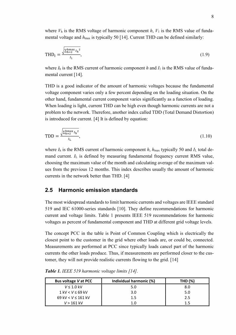
current and voltage limits. Table 1 presents IEEE 519 recommendations for harmonic

voltages as percent of fundamental component and THD at different grid voltage levels.

The concept PCC in the table is Point of Common Coupling which is electrically the

closest point to the customer in the grid where other loads are, or could be, connected.

Measurements are performed at PCC since typically loads cancel part of the harmonic

currents the other loads produce. Thus, if measurements are performed closer to the cus-

tomer, they will not provide realistic currents flowing to the grid. [14]

Table 1. IEEE 519 harmonic voltage limits [14].

Bus voltage V at PCC Individual harmonic (%) THD (%)

V ≤ 1.0 kV 5.0 8.0 1 kV ˂ V ≤ 69 kV 3.0 5.0

69 kV ˂ V ≤ 161 kV 1.5 2.5 V > 161 kV 1.0 1.5

9

The short time values (average of 10 minutes) should be less than the values in Table 1

95 percent of the time weekly. Very short time values (average of 3 seconds) should be

less than 1.5 times the values in the table for 99 percent of the time daily. [14]

In IEEE 519 current distortion limit recommendations are given for different system volt-

age levels. Because high voltage systems are studied in this thesis, only their limits are

shown here. Table 2 presents recommended current distortion limits for systems rated

from 69 kV to 161 kV. Individual harmonic currents are expressed in percent of the total

demand current IL. The limits in the table are for odd harmonics only. Even harmonic

components are limited to 25 percent of the odd harmonic limits. Recommendations vary

also as a function of ISC/IL. ISC means the short-circuit current at PCC. For all power

generation equipment, the current limits are the first-row limits regardless of the actual

ISC/IL-ratio. [14]

Table 2. IEEE 519 harmonic current limits for systems rated from 69 kV to 161 kV [14].

Individual harmonic component h in percent of IL

ISC/IL 3 ≤ h ˂ 11 11 ≤ h ˂ 17 17 ≤ h ˂ 23 23 ≤ h ˂ 35 35 ≤ h ≤ 50 TDD

˂20 2.0 1.0 0.75 0.3 0.15 2.5 20 - 50 3.5 1.75 1.25 0.5 0.25 4.0

50 - 100 5.0 2.25 2.0 0.75 0.35 6.0 100 - 1000 6.0 2.75 2.5 1.0 0.5 7.5

˃1000 7.5 3.5 3.0 1.25 0.7 10.0

Weekly 95 percent of the short time (10 minutes) harmonic currents should be less than

the values given in Table 2. Weekly 99 percent of the short time (10 minutes) harmonic

currents should be less than 1.5 times the values in the table and daily 99 percent of the

very short values (3 seconds) should be less than 2.0 times the values in the table. [14]

Table 3 presents recommended current distortion limits for systems rated above 161 kV.

The clarifications made for lower voltage level systems apply for them also.

Table 3. IEEE 519 harmonic current limits for systems rated above 161 kV [14].

Individual harmonic component h in percent of IL

ISC/IL 3 ≤ h ˂ 11 11 ≤ h ˂ 17 17 ≤ h ˂ 23 23 ≤ h ˂ 35 35 ≤ h ≤ 50 TDD

˂20 1.0 0.5 0.38 0.15 0.1 1.5 20 - 50 2.0 1.0 0.75 0.3 0.15 2.5

≥50 3.0 1.5 1.15 0.45 0.22 3.75

IEC 61000-series includes a few standards which define limits for harmonics. IEC 61000-

2-2 defines compatibility levels for harmonic voltages in low voltage networks [15] and

IEC 61000-2-4 defines compatibility levels for harmonic voltages in industrial plants at

10

nominal voltages up to 35 kV [16]. IEC 61000-2-12 defines compatibility levels for har-

monic voltages in medium voltage power systems from 1 kV to 35 kV [17].

IEC 61000-3-2 sets limits for harmonic current emissions for equipment which input cur-

rent is equal or below 16 amperes [18] and IEC 61000-3-12 for equipment which input

current is between 16 and 75 amperes [19]. Both standards are for low voltage networks.

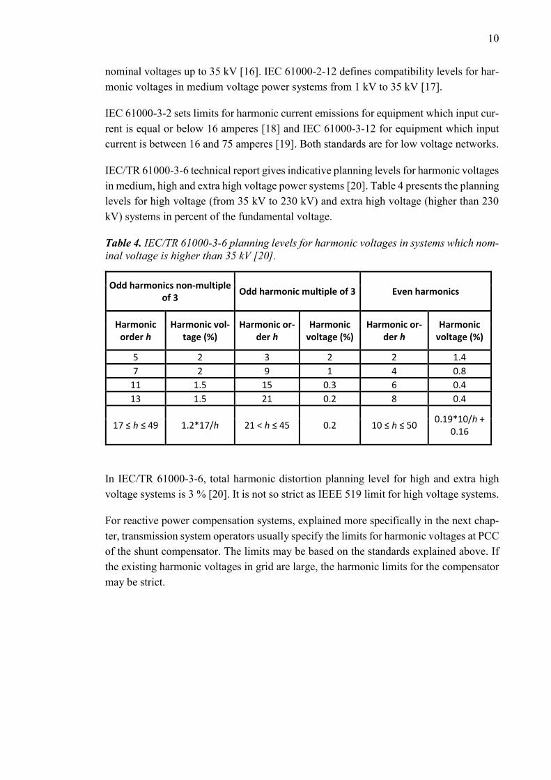
IEC/TR 61000-3-6 technical report gives indicative planning levels for harmonic voltages

in medium, high and extra high voltage power systems [20]. Table 4 presents the planning

levels for high voltage (from 35 kV to 230 kV) and extra high voltage (higher than 230

kV) systems in percent of the fundamental voltage.

Table 4. IEC/TR 61000-3-6 planning levels for harmonic voltages in systems which nom-

inal voltage is higher than 35 kV [20].

Odd harmonics non-multiple of 3

Odd harmonic multiple of 3 Even harmonics

Harmonic order h

Harmonic vol-tage (%)

Harmonic or-der h

Harmonic voltage (%)

Harmonic or-der h

Harmonic voltage (%)

5 2 3 2 2 1.4

7 2 9 1 4 0.8

11 1.5 15 0.3 6 0.4

13 1.5 21 0.2 8 0.4

17 ≤ h ≤ 49 1.2*17/h 21 < h ≤ 45 0.2 10 ≤ h ≤ 50 0.19*10/h +

0.16

In IEC/TR 61000-3-6, total harmonic distortion planning level for high and extra high

voltage systems is 3 % [20]. It is not so strict as IEEE 519 limit for high voltage systems.

For reactive power compensation systems, explained more specifically in the next chap-

ter, transmission system operators usually specify the limits for harmonic voltages at PCC

of the shunt compensator. The limits may be based on the standards explained above. If

the existing harmonic voltages in grid are large, the harmonic limits for the compensator

may be strict.

11

3. REACTIVE POWER COMPENSATION

Like harmonics, reactive power flow is an undesired phenomenon in power systems.

However, reactive power is needed to build magnetic fields for example in transformers,

generators and motors. This reactive power type is called inductive. Reactive power is

also needed to build electric fields for example in capacitors. This type of reactive power

is called capacitive. Reactive power is not converted into heat, light or torque like active

power but fluctuates between capacitive and inductive loads. Still it increases the current

flowing in the network. [21] Due to growth of current, transmission system losses increase

[22]. Reactive power should be compensated for various reasons such as to increase ac-

tive power transmission capacity in the grid, to keep the grid node voltages in the desired

limits, to improve stability of the network and to mitigate power oscillations [23].

In this chapter, the definition of reactive power, principles of its compensation and dif-

ferent compensation solutions are introduced. Basic compensation solutions are passive

shunt and series compensators. Modern compensators are based on power electronics.

The most common power electronic compensators are SVC (Static Var Compensator)

and STATCOM (Static Synchronous Compensator) which are introduced. Studied

STATCOM topology in this thesis is MMC (Modular Multilevel Converter) whose oper-

ation is described. The basics of STATCOM’s control system and modulator are also

explained. Compensators have different harmonic current emissions and effect on reso-

nances which are described for each compensator.

3.1 Reactive power

Reactive power definition can be derived from instantaneous power p which is

𝑝(𝑡) = 𝑣𝑖, (3.1)

where v is instantaneous value of voltage and i instantaneous value of current. The aver-

age value of power is called active power P and assuming sinusoidal voltage and current

it is

𝑃 = 𝑉𝐼 cos(𝜑V − 𝜑I), (3.2)

where V is the RMS value of voltage, I the RMS value of current, φV voltage angle and

φI current angle.

The instantaneous power includes a term oscillating at twice the frequency of current and

voltage and whose average is zero. The peak value of this oscillating power is called

reactive power Q: [21]

12

𝑄 = 𝑉𝐼 sin(𝜑V − 𝜑I). (3.3)

Reactive power is positive and called inductive if voltage leads current and negative and

called capacitive if current leads voltage. There is also a third power term called apparent

power S which is the product of voltage and current RMS values:

𝑆 = 𝑉𝐼. (3.4)

The following relation applies for powers:

𝑆 = √𝑃2 + 𝑄2. (3.5)

Increased reactive power means thus increased apparent power and current. When voltage

and current contain harmonics, also instantaneous power includes harmonics. In a com-

mon definition, reactive power still refers to reactive power caused by fundamental fre-

quency variables and harmonics are considered in additional power term called distortion

power [21].

3.2 Passive shunt compensators

Many loads draw inductive reactive power from the network. A simple way to compen-

sate it is to connect a capacitor as shunt to the transmission line. Shunt compensation

principle is shown in Figure 7.

Figure 7. Principle of shunt compensation, a) situation without compensation, b) with

compensation [23].

In Figure 7. a) load is inductive-resistive which means that current I lags voltage V2. Cur-

rent has an active current component IP and a reactive component IQ which of whom the

latter should be compensated. In Figure 7. b) current source is added parallel to the load

having the same reactive component magnitude IQ as the load but a 180-degree phase

shift. This capacitive current component cancels the inductive current drawn by the load.

The resulting current drawn from the grid has only an active component which means that

only active power is transferred. Because total current is smaller, power losses decrease.

Therefore, more active power can be transmitted with same losses.

13

As capacitive current is needed for compensation, a capacitor can be used instead of cur-

rent source. However, capacitor current IC and thus supplied reactive power QC depend

on grid voltage V at its connection point according to the equations below.

𝐼C =𝑉

𝑋C, (3.6)

𝑄C = 𝑉𝐼C =𝑉2

𝑋C, (3.7)

where XC is the capacitive reactance of the capacitor. If voltage varies, also supplied re-

active power varies. Thus, the reactive power consumed by the load will not be compen-

sated fully if it does not change likewise.

Shunt capacitors can be fixed or mechanically switched. In a fixed capacitor bank the

capacitance is not controllable. A switched capacitor bank consists of multiple capacitor

units which can be switched on and off individually. Therefore, amount of capacitive

reactance and supplied reactive power can be controlled. However, mechanical switches

(circuit breakers) are quite slow and can not be switched on and off many times a day, so

capacitors having mechanical switches can not be used for dynamic compensation of rap-

idly changing loads. [22]

In transmission networks the objective is not to compensate reactive power of single

loads. Purpose is to impose an optimal voltage profile in grid nodes so that grid transfer

capability would be maximized, losses minimized and high voltage stability achieved

[22]. Reactive power affects grid voltages which can be shown by considering a simple

grid consisting of two nodes. Grid and phasor diagram of its voltages and currents are

presented in Figure 8.

Figure 8. a) Simple grid and b) phasor diagram of its variables to illustrate reactive

power effect on voltage [22].

In the diagram load is inductive-resistive so the angle difference φ between 𝜐2̅ and 𝜄 ̅ is

positive. The current components are 𝐼P = 𝐼cos𝜑 and 𝐼Q = 𝐼sin𝜑 and for inductive loads

𝜄 ̅ = 𝐼P − 𝑗𝐼Q, where j is the imaginary operator. The complex voltage drop in grid imped-

ance has real and imaginary components:

14

∆𝑢 = 𝑅𝐼P + 𝑋𝐼Q, (3.8)

𝛿𝑢 = 𝑋𝐼P − 𝑅𝐼Q, (3.9)

which are shown in the phasor diagram [22]. Complex power in one phase is

𝑆 = 𝑉n2(𝐼P + 𝑗𝐼Q) = 𝑃 + 𝑗𝑄, (3.10)

where Vn2 is voltage at node 2. Equations 3.8 and 3.9 can be written as a function of

powers as follows:

∆𝑢 =𝑅𝑃+𝑋𝑄

𝑉2, (3.11)

𝛿𝑢 =𝑋𝑃−𝑅𝑄

𝑉2. (3.12)

Because transmission grid’s resistance is usually much smaller than reactance, the voltage

drop components become [22]

∆𝑢 ≈𝑋𝑄

𝑉2, (3.13)

𝛿𝑢 ≈𝑋𝑃

𝑉2. (3.14)

Voltage drop magnitude, which is close to Δu, is mainly affected by reactive power in-

jected from node 1 to node 2 and phase difference between node voltages is mainly af-

fected by active power flow between nodes [22]. Grid impedance is usually inductive-

resistive at fundamental frequency, which means that X is positive. When load is capaci-

tive instead of inductive the reactive power changes polarity from positive to negative.

Voltage drop is then negative and voltage at node 2 is higher than at node 1. This means

that capacitors can be used to increase voltage at the nodes they are placed. When the

capacitive reactive power propagates further, it increases also the voltages at the nodes

near the node where capacitor is placed according to the same equations.

Shunt capacitors can be used to support voltage but they have some disadvantages. As

mentioned they are either fixed or mechanically switched and thus can not be used for

dynamic voltage compensation. Another problem of shunt capacitor is that it is used to

support voltage but as voltage decreases, its reactive power output decreases proportional

to voltage squared according to equation 3.7 [22]. Also, as the load is light and voltage

high, capacitor’s reactive power output increases which increases the voltage even more

[22].

Capacitor itself is not a suitable compensator because of the resonance phenomenon de-

scribed in chapter 2.3. To avoid resonances with the inductive network a reactor must be

connected in series with the capacitor. The reactor and capacitor form a series resonance

15

circuit which is tuned typically to 189 Hz in 50 Hz grid. The series connection absorbs a

small portion of the fifth and seventh harmonic currents. The tuning frequency of 189 Hz

is normally the most economical choice considering the needed amount of reactor mate-

rial. [21]

Moreover, when capacitor bank is energized or grid voltage changes fast in transient sit-

uations, capacitor current changes stepwise to a large value according to basic relation of

capacitor voltage and current:

𝑖cap(𝑡) = 𝐶𝑑𝑣cap(𝑡)

𝑑𝑡, (3.15)

where icap is the capacitor current, C capacitance, vcap capacitor voltage and t time. This

high current flowing through the grid causes oscillations in grid voltage. Adding the series

reactor reduces this inrush current and voltage oscillations. [24]

Shunt compensators can be designed to supply reactive power and act also as harmonic

filters to improve power quality. In this case, their impedances are capacitive at frequen-

cies below the tuning frequency and inductive above the tuning frequency. The idea is to

compensate reactive power at fundamental frequency and offer a low impedance path for

some harmonic currents so that they would flow to the filter instead of grid. [21]

There are many different filter configurations. Some of the basic configurations are pre-

sented in Figure 9.

16

Figure 9. Typical harmonic filters and their impedances: a) tuned filter, b) second order

damped filter and c) C-type filter [25].

The simplest of the filters is a tuned filter which consists of a series connection of capac-

itor and reactor. At the tuning frequency of series connection, the impedance of the filter

is only the resistance of the reactor [25]. The tuning frequency is chosen to be almost the

frequency of desired harmonic to be filtered but not precisely to avoid extremely high

c) C-type filter

b) Second order damped filter

a) Tuned filter

17

currents flowing to the filter [21]. The advantages of a tuned filter are that it is simple, it

offers optimum attenuation for one harmonic current and its losses are low. Its disad-

vantages are that multiple filters are needed if many harmonics need attenuation and its

tuning frequency is susceptible to de-tuning factors such as component manufacturing

tolerances, temperature changes and grid frequency variations. The de-tuning can be

avoided by making the inductance adjustable using inductor taps but that increases costs.

[25]

A second order damped filter is similar to tuned filter but a resistor is connected in parallel

with the reactor. This addition reduces the impedance magnitude dip at the tuning fre-

quency but broadens the dip around it. The advantages of a damped filter are that it can

attenuate multiple harmonics at the same time and the broadened impedance dip means

that the attenuation at desired frequency is not so sensitive to de-tuning factors. Disad-

vantages are the reduced attenuation at the tuning frequency and higher losses at both

fundamental and harmonic frequencies because of the added resistor. [25]

In a C-type filter second capacitor is added in series with the reactor. Second capacitor

and inductor form a series resonance at the fundamental frequency and thus all funda-

mental current flows through the series connection instead of resistor. Advantage is that

losses at the fundamental frequency are minimized. Disadvantage is that the LC-circuit

resonance frequency may change because of the previously mentioned de-tuning factors

and then the current flows also through the resistor. Thus, resistor needs to be rated for

part of the fundamental current also or the inductor needs to be adjustable. Also, the har-

monic attenuation is slightly worse than with second order damped filter. [25]

Adding a filter to the network may cause parallel resonances between the filter and net-

work. The impedance of the filter is capacitive below the tuning frequency and the grid

impedance is usually inductive. This means that parallel resonance might occur at some

frequency below the tuning frequency. [21] The possible resonances should be considered

in filter design. Usually the customer specifies the network harmonic impedances which

will change over time because of different system configurations and connection and dis-

connection of loads and generators. Often the network impedances are presented as im-

pedance envelopes such as sector or circle diagrams that include all the possible imped-

ance values. [25] Using this data possible resonances can be identified.

3.3 Passive series compensators

Reactive power can be compensated also by adding a capacitor in series with the trans-

mission line. The idea is to decrease the inductive reactance of the power line at the fun-

damental frequency and consequently decrease the absorbed inductive reactive power in

the line [23]. Series capacitor with its protection system is shown in Figure 10. Typically,

a metal oxide varistor, a spark gap and a fast bypass switch are used as overvoltage pro-

tection for the compensator [23].

18

Figure 10. Series capacitor compensator and its protection system [23].

Active power transmitted through the transmission line is without compensation

𝑃 =𝑉n1𝑉n2 sin𝛿

𝑋L, (3.16)

where Vn1 is voltage magnitude at node 1, Vn2 voltage magnitude at node 2, δ voltage

angle difference between nodes 1 and 2 and XL is inductive reactance of the line [26].

When capacitor is added, the transmitted power is

𝑃 =𝑉n1𝑉n2 sin𝛿

𝑋L−𝑋C, (3.17)

where XC is the capacitive reactance of the capacitor bank. Adding the capacitor bank

thus increases the active power transmission capacity. [26] If the inductive reactance is

fully compensated, meaning XC=XL, a series resonance occurs at fundamental frequency

[27]. To avoid very large fundamental current, it is not recommended to compensate more

than 80 % of the reactance [27].

3.4 SVC

Static Var Compensator (SVC) is a controllable shunt compensator based on power elec-

tronic switches. Typically, it consists of a step-down transformer, thyristor-controlled re-

actors (TCRs), thyristor-switched capacitors (TSCs) and harmonic filters [28]. A typical

SVC configuration is presented in Figure 11. Because of controllable thyristor switches,

shunt reactance and reactive power output of SVC can be controlled [29]. That makes it

possible to control also the PCC voltage as equation 3.13 states.

19

Figure 11. Typical SVC configuration.

TCR consists of anti-parallel connected pair of thyristor valves in series with a reactor.

One of the thyristor valves conducts positive half-waves of current and the other negative

half-waves. The starting of current flow is determined by the thyristor firing angle which

is measured from the moment of voltage zero crossing. In TCR, thyristor firing angles are

controlled from 90 to 180 degrees. 90° angle means that the reactor current is continuous

and 180° that the thyristors do not conduct at all. The current flow of thyristor ceases

naturally as it reaches zero. The firing angle determines the impedance of TCR seen from

the connection point. Consequently, fundamental inductive current component changes

as the applied voltage magnitude is constant. However, when firing angle is between 90

and 180 degrees, the reactor current is non-sinusoidal and harmonics are generated. [28]

The harmonics in phase current produced by symmetrically controlled three-phase delta-

connected TCR are presented as a function of firing angle in Figure 12. Harmonics are

expressed in percent of produced fundamental frequency phase current.

TCR TSC5th filter 7th filter

Step-down transformer

PCC

20

Figure 12. Harmonic current emissions of symmetrically controlled delta-connected

three-phase TCR as a function of thyristor firing angle [28].

As can be seen, different harmonics do not peak at the same firing angle. When both anti-

parallel thyristor valves are fired with same firing angle, the even harmonic currents do

not exist. When three TCRs are connected in delta and are controlled symmetrically, the

produced triplen harmonics (3, 9, 15, …) are equal in each branch and thus circulate in

the delta and do not flow into the network. Because the TCR produces quite large har-

monics at especially 5th and 7th harmonics, harmonic filters are usually needed. The filters

also provide capacitive reactive power at fundamental frequency. [28]

TSC consists of anti-parallel connected pair of thyristor valves in series with a capacitor

and current limiting reactor. As described earlier for passive shunt compensators, capac-

itor needs the small reactor to limit the current in overvoltage and switching situations.

The reactor is usually chosen so that the series resonance frequency of the circuit is be-

tween the 4th and 5th harmonic. This ensures that TSC does not create a resonance circuit

with the network at some harmonic frequency. The thyristors are only switched on or off

so there is not firing angle control as in TCR. This also means that the current of TSC is

sinusoidal in steady-state. [28]

3.5 STATCOM

Static Synchronous Compensator (STATCOM) is also a shunt compensator based on

power electronic switches but its operating principle differs from SVC’s. STATCOM is

a controllable voltage source behind a reactor [2]. It can produce its rated inductive and

capacitive reactive current independent of grid voltage whereas SVC’s maximum reactive

current depends linearly on grid voltage [2]. Other STATCOM advantages over SVC are

smaller size, faster response, and possibility to have short-term transient overload capa-

bility [2]. Also, harmonic current emissions are lower especially with STATCOM based

on multilevel converter [23]. STATCOM is however more expensive [30].

21

3.5.1 Operating principle

STATCOM consists of a coupling or step-down transformer, a coupling reactor and a

voltage source converter. The voltage source converter is comprised of a capacitor energy

storage and a DC-AC converter. [2] Basic configuration of STATCOM is presented in

Figure 13 with phasor diagrams of its electrical variables in capacitive and inductive op-

erating points.

Figure 13. STATCOM, a) basic configuration, b) phasor diagrams in capacitive and in-

ductive operating points [2].

STATCOM’s reactive power generation is based on the voltage magnitude difference

between grid connection point voltage V and converter produced voltage E. If losses are

neglected, converter produces three-phase voltages in phase with the grid three-phase

voltages. Then, the drawn reactive current in one phase is

𝐼Q =𝑉−𝐸

𝑋, (3.18)

where X is the sum of transformer and coupling reactor reactances [2]. The reactive power

drawn from the grid is therefore [2]

𝑄 = 𝑉𝐼Q =1−

𝐸

𝑉

𝑋𝑉2. (3.19)

By controlling the magnitude of produced voltage E, the reactive power output can be

controlled. When the produced voltage magnitude is larger than grid voltage magnitude,

resulting current is leading grid voltage and the converter generates capacitive reactive

power. If the produced voltage magnitude is smaller than grid voltage, lagging current is

a)

b)

22

produced and inductive reactive power is absorbed. [2] Resulting currents in both situa-

tions are illustrated in phasor diagrams in Figure 13.

In a real STATCOM, there are losses in converter switches which causes the capacitor

energy to discharge. The energy to cover these losses can be supplied from the grid by

making the converter produced voltage lag the grid voltage by a small angle as equation

3.16 indicates. The capacitor voltage can be thus kept in desired limits. [2]

There are different topologies, switching devices and switching strategies used in the

voltage-source converter of STATCOM. Basic topologies are two-level, three-level and

multilevel converters, where the level corresponds to the number of possible voltage out-

put levels in one phase of the converter. Common switching devices are GTO (Gate-Turn-

Off) thyristor, IGBT (Insulated Gate Bipolar Transistor) and IGCT (Integrated Gate Com-

mutated Thyristor). GTO thyristor is rated for higher currents but IGBT and IGCT have

faster response times and lower switching losses. [31]

In low-level converters, switching of a single switch on and off can be done once or many

times in a fundamental cycle. If it is done many times, switching pattern is achieved by

comparing a sinusoidal reference signal and a high-frequency triangle carrier. This

switching method is called PWM (Pulse Width Modulation). If switching is done only

once in a fundamental cycle, harmonics in produced voltage will be large. This can be

overcome by having multiple converters connected parallel, triggering the switches of

parallel converters with appropriate displacement angles with respect to each other and

summing the produced voltages together using appropriate transformer connections. The

result is a multilevel voltage waveform at transformer primary which approximates a si-

nusoid. When PWM is used in low-level converters, the voltage waveform will be closer

to sinusoid which decreases the harmonic voltages. However, the switching losses in

high-power low-level converters are large and thus PWM is not generally used in them.

In multilevel converters, the desired voltage is produced from several capacitor DC-volt-

age sources. Thus, low harmonic distortion in voltage can be achieved with fundamental

frequency switching of individual converter if the level number is high enough. [31]

Common for all the voltage-source converters is that the produced voltage only approxi-

mates a sinusoid. Thus, there are harmonics in output voltage. The harmonic voltages

cause harmonic currents to be drawn from the grid [2]. Harmonic currents decrease as a

function of frequency because of the increasing reactances in transformer and coupling

reactor [2].

3.5.2 Modular Multilevel Converter

Modular Multilevel Converter (MMC) is a common multilevel converter type which can

act as a voltage source in STATCOM. It consists of a series connection of submodules in

each of the three phases. One submodule, called full-bridge, is comprised of four switches

23

and one capacitor. A switch is typically an IGBT and a diode connected anti-parallel

which enables current flow to both directions. One full-bridge submodule can produce

three output voltage levels +VDC, 0 or -VDC, where VDC is the voltage in the submodule

capacitor. The total voltage of the series connection is the sum of individual submodule

voltages. Therefore, it is possible to produce 2n+1 voltage levels in one phase, where n is

the number of series-connected submodules. Submodules are switched so that a staircase

voltage waveform is produced which approximates a sinusoid. The single-phase series-

connected structures can be connected in star- or delta-configuration to form a three-phase

converter. [32] MMC configurations are shown in Figure 14. In this thesis, STATCOM

based on MMC with full-bridge submodules connected in delta-configuration is studied.

Figure 14. MMC, a) star-configuration, b) delta-configuration [33].

In medium and high voltage applications, MMC has several advantages compared to con-

ventional two-level converters that use high switching frequency pulse width modulation.

The switches can be rated based on the submodule capacitor voltages which are substan-

tially smaller than full DC-link voltage in a two-level converter. In MMC, output voltage

with low harmonic distortion can be produced without high switching frequencies. Be-

cause switching causes losses, MMC’s losses are smaller than those of two-level convert-

ers. In high voltage levels, high voltage blocking capability is needed in two-level con-

verter switches which increases the losses in one switching action. Switching frequency

of those converters must be limited to about 1 kHz due to high losses which means in-

creased harmonic voltages. [34] In MMC submodules are identical and can be connected

in series to form modules with desired total voltage levels. This modularity enables

cheaper and faster manufacturing. [32] Fault tolerance can be enhanced by adding redun-

dant submodules in series so that faulty submodules can be bypassed [34].

Disadvantage of MMC is that a great number of semiconductor switches with gate drive

circuits are needed. That makes the system more complex and expensive. [32] In a two-

24

level converter, all phases are connected to a common DC-link so there is no need for

power balancing between phases. In MMC, all submodules have a capacitor energy stor-

age and their energies must be actively balanced. [34]

3.5.3 Control system

Despite the simple principle of reactive power compensation in STATCOM and simple

modular structure of MMC, quite complex control system is needed to achieve good and

stable performance. In this subchapter, the overall control block diagram of studied

STATCOM is presented and the purpose of each block is shortly described. In this thesis,

a balanced three-phase system is assumed which means that the magnitudes of three-

phase voltages are equal and their phase shifts are exactly 120 degrees. Therefore, control

system characteristics related to unbalanced grid conditions are not introduced here.

The control is partly done in synchronous reference frame and partly in three-phase frame

(abc-frame). Three-phase voltage and current can be transformed to αβ-frame and then to

synchronous reference frame (dq-frame). For voltage, the transformation from abc- to αβ-

frame is [34]

[

𝑣α

𝑣β

𝑣0

] =

[ 2

3−

1

3−

1

3

01

√3−

1

√31

3

1

3

1

3 ]

[

𝑣a

𝑣b

𝑣c

], (3.20)

where vα is voltage α-component, vβ voltage β-component, v0 zero sequence voltage, va

instantaneous value of phase a voltage, vb instantaneous value of phase b voltage and vc

instantaneous value of phase c voltage. Zero sequence voltage can be neglected in bal-

anced three-phase system. The axes α and β are 90 degrees shifted from each other and

thus form a complex plane. The three-phase voltage can be presented as a space vector

which rotates counterclockwise with the fundamental angular frequency ω1 in the plane:

[34]

𝒗𝛂𝛃 = 𝑣α + 𝑗𝑣β. (3.21)

The magnitude of the vector is same as the peak value of phase voltage. Synchronous

reference frame is also a complex plane which rotates to same direction as space vector

with the fundamental angular frequency. Thus, in synchronous frame, space vector is

standing still. [34] For voltage, the transformation from αβ- to dq-frame is

[𝑣d

𝑣q] = [

cos 𝜃 sin 𝜃−sin 𝜃 cos 𝜃

] [𝑣α

𝑣β], (3.22)

25

where vd is voltage d-component, vq voltage q-component and θ the transformation angle

which is chosen so that frame’s d-axis is aligned with the voltage vector [34]. The voltage

vector in dq-frame is

𝒗𝐝𝐪 = 𝑣d + 𝑗𝑣q. (3.23)

Transformation matrices are the same for current. Inverse transformation from dq- to abc-

frame can be derived from equations 3.20 and 3.22. In Figure 15 voltage and current

vectors in stationary and synchronous frames are illustrated. In stationary frame, the vec-

tors rotate and in synchronous frame the dq-frame rotates with angular speed ω1.

Figure 15. Voltage and current vectors in a) stationary frame, b) synchronous frame.

When dq-frame is aligned with the voltage vector, voltage d-component is equal to volt-

age magnitude and q-component is zero. Then, instantaneous active power p is [34]

𝑝 =3

2𝑣d𝑖d (3.24)

and instantaneous reactive power q is [34]

𝑞 = −3

2𝑣d𝑖q. (3.25)

According to the equations, active power depends on current d-component and reactive

power depends on current q-component. Thus, it is possible to control powers inde-

pendently. [34]

STATCOM’s control block diagram is shown in Figure 16 and in larger size in Appendix

A, Figure 1. Also, the explanations for diagram abbreviations are given in the appendix.

The control cycle shown in the diagram is executed at 10 kHz frequency.

α

β

d

q

v

i

ω1

β

v

i

α

ω1

ω1

a) b)

26

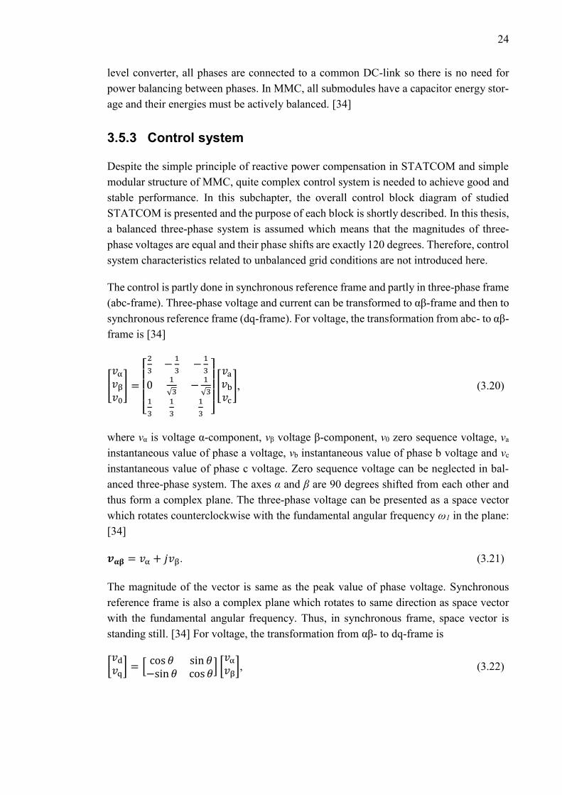
Figure 16. Control block diagram of STATCOM.

One synchronization block tracks PCC line-to-neutral voltage fundamental frequency d-

component by controlling voltage q-component to zero. The block calculates voltage d-

component magnitude from the measured voltage which is equal to fundamental voltage

magnitude. Another synchronization block tracks the line-to-line voltage of secondary

busbar. It produces the transformation angle θ which is used in the dq-to-abc transfor-

mation.

Voltage controller produces current q-component reference by controlling the difference

between PCC voltage magnitude reference and measured PCC voltage fundamental com-

ponent magnitude to zero. Current q-component can be used for reactive power control

according to equation 3.25 and PCC voltage can be controlled by produced or absorbed

reactive power as equation 3.13 states. As the reference is a DC-value, PI-controller (pro-

portional-integral controller) can be used to track it [34]. Another option is to use manual

control where current q-component reference is set manually.

The total DC-voltage in each delta branch should be kept close to nominal value so that

desired output voltages can be produced. The losses in switches cause the capacitors’

voltages to decrease so active power is needed from grid to compensate the losses as

described earlier. There are two controllers to perform this task. First PI-controller con-

trols the average DC-voltage of three branches to the nominal value by producing the

current d-component reference. Still, there might be unbalance between DC-link branch

voltages if grid voltage is unbalanced. Branch voltages can be balanced by forcing an

appropriate zero sequence current to circulate in delta connection [34]. Second controller

produces the current zero sequence component reference.

Synchroni-zation to

PCC voltage

PCC voltage

controller

Current controller

Current reference generator

DC-link voltage

controllers

Voltage reference generator

Modulator

vpcc,LN,meas

vpcc,magn,ref

Measured submodule

voltages

vd,meas

iq,ref

id,ref

i0,ref iMMC,ref

Manual iq-

control

iq,ref

θ

vsec,LL,measiMMC,meas

vMMC,ref

Submodule states

(+1, 0 or -1)

Measured submodule

voltages

iMMC,meas

Synchronization to secondary

busbar voltage

vsec,LL,meas

Synchronous frame Stationary frame

(optionally)

27

Current reference generator forms the reference current for MMC in abc-frame from the

current reference d-, q- and zero-sequence components. The transformation angle pro-

duced by synchronization block is used in the transformation. MMC is connected in delta-

configuration, so the references are calculated for each delta branch.

There are three current controllers, one for each delta branch which control the difference

between current references and measured MMC branch currents to zero. PI-controllers

can not track sinusoidal reference signals, so PR-controllers (proportional-resonant con-

trollers) are used which can perform the task [35]. PR-control theory is more discussed

in chapter 5.2.

Voltage reference generator generates the three-phase voltage reference for MMC. The

reference for each delta-branch is calculated by subtracting the current controller output

from the measured secondary busbar voltage. This voltage feedforward can be either in-

stantaneous three-phase voltage with all the harmonics or only the fundamental compo-

nent. These two feedforward options are compared later in this thesis from the viewpoint

of produced harmonic currents.

Finally, modulator is needed to transform the voltage references to information which

submodules in each branch should be connected and which bypassed. Modulator’s out-

puts are the states of each submodule: +1, 0 or -1. State +1 means that the submodule

should produce +VDC voltage at its terminals, state -1 means that it should produce -VDC

voltage at its terminals and state 0 that the module must be bypassed.

In addition to reference voltage production, modulator must balance individual submod-

ule DC-voltages in each branch. The voltage of a submodule stays unchanged when it is

bypassed but increases or decreases when it is connected to AC-terminals depending on

the power flow direction [34]. Without balancing that would lead to large voltages in

some submodules and small voltages in some submodules. Large voltages could break

the capacitors. A logic for choosing the submodule to be connected or bypassed is based

on the power flow direction and the measured submodule voltages.

28

4. HARMONIC CURRENTS AND VOLTAGES OF

STATCOM

STATCOM model implemented in PSCAD simulation program was used to simulate the

harmonic current emissions of STATCOM. In the simulation model, modular multilevel

converter is modelled as voltage source whose three-phase voltage is produced by control

system and modulator described in chapter 3.5.3. Changes of submodule DC-voltages are

calculated every simulation step according to equation 3.15. STATCOM model includes

also the coupling reactor and its parasitic resistance, transformer model, measurements

and some additional protection functions not meaningful in steady-state operation. Grid

is modelled as series connection of voltage source and impedance. Harmonic currents and

voltages were extracted from measured waveforms using Fast Fourier Transform block

provided by PSCAD and exported to Excel for calculations and graph drawing.

First, STATCOM’s current was simulated when grid voltage was sinusoidal at fundamen-

tal frequency 50 Hz. Then, harmonics were added to grid voltage and simulation was

repeated to illustrate the increasing harmonic currents of STATCOM. Goal was to find

out how harmonic current emissions affect harmonic voltages at PCC which are limited

by standards and transmission system operators’ specifications. The harmonic current

mitigation performance of increased reactances in coupling reactor and transformer were

also illustrated. In all simulations, manual current q-component control was used. As de-

scribed in chapter 3.5.3, this current component affects the reactive power output of

STATCOM and thus PCC voltage. To see if operating point has any effect on harmonic

currents, capacitive, inductive and zero current reference situations were simulated.

4.1 Harmonic current emissions with sinusoidal grid voltage

In the first simulations grid voltage was sinusoidal at 50 Hz. Grid positive sequence volt-

age was 138 kV and there was no negative sequence voltage. Transformer’s connection

was YNd11 and its secondary nominal voltage was set to 34.5 kV. Used grid resistance

and reactance at fundamental frequency were 0.9292 Ω and 9.477 Ω, respectively. Grid

impedance corresponds to 2000 MVA short-circuit level at PCC. Used transformer reac-

tance was 0.115 p.u (per unit). STATCOM’s rated power was 100 MVAr and it consisted

of 40 submodules per branch. All grid and STATCOM parameters used in the simulations

are shown in Appendix B, Table 1. The configuration used in the simulations is illustrated

as single line diagram in Figure 17.

29

Figure 17. Single line diagram of the circuit used in the first simulations.

As explained in chapter 3.5.3, STATCOM’s voltage reference is calculated by subtracting

the current controller’s output from the feedforward of secondary busbar voltage. The

two feedforward options considered are fundamental voltage and instantaneous voltage

feedforward. Fundamental voltage feedforward means that only fundamental component

of the secondary busbar voltage is used. Instantaneous voltage feedforward means that

the measured secondary busbar voltage, including all the harmonics, is used. In the sim-

ulations with sinusoidal grid voltage, fundamental feedforward was used. However, feed-

forward method has not a great significance on harmonic performance when grid voltage

is sinusoidal. Only harmonic currents produced by STATCOM cause harmonic voltages

to the secondary busbar.

First, simulation was done in capacitive operating point. The current q-component refer-

ence was set to 1.0 p.u which means 1000 A fundamental frequency capacitive current in

STATCOM’s delta branch. A-phase current at PCC was simulated for 1 second. Har-

monic current spectrum changes a bit as function of time so average of the harmonic

currents was taken from interval 0.9 s to 1.0 s. This averaging was used in all following

simulations. Figure 18 presents the harmonic spectrum of PCC current in a-phase. To

compare different operating points, the harmonic currents were calculated as percent of

the used fundamental frequency current maximum. Used fundamental component maxi-

mum was √3*1000 A in one phase in secondary which is converted to primary using ratio

of secondary nominal voltage 34.5 kV to primary nominal voltage 138 kV.

Transformer, 138 kV / 34.5 kV

G

Ideal voltage source, 50 Hz

DGrid resistance and reactance

PCC

Y

30

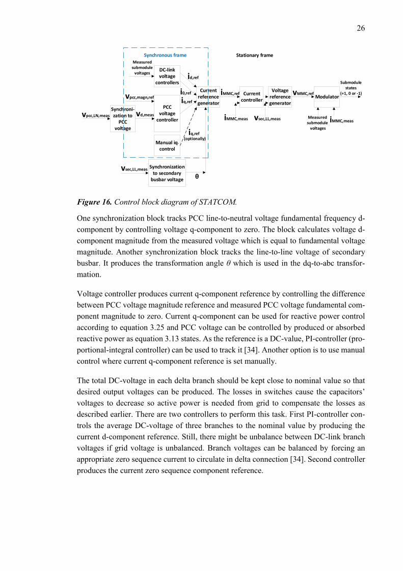
Figure 18. Harmonic spectrum of PCC current in capacitive operating point in sinusoi-

dal grid.

Calculated current TDD was 0.038 % when all 100 harmonic components were consid-

ered. The current distortion is very low and does not usually cause any problems.

Next, simulation was done in inductive operating point. The current q-component refer-

ence was set to -1.0 p.u which means 1000 A fundamental frequency inductive current in

STATCOM’s delta branch. Same parameters were used as for capacitive operating point.

A-phase harmonic currents at PCC are presented in Figure 19.

Simulation was also done in zero current operating point. The current q-component ref-

erence was set to 0 p.u which means 0 A fundamental frequency current in STATCOM’s

delta branch. Figure 20 shows the harmonic spectrum of PCC current in a-phase.

Figure 19. Harmonic spectrum of PCC current in inductive operating point in sinusoidal

grid.

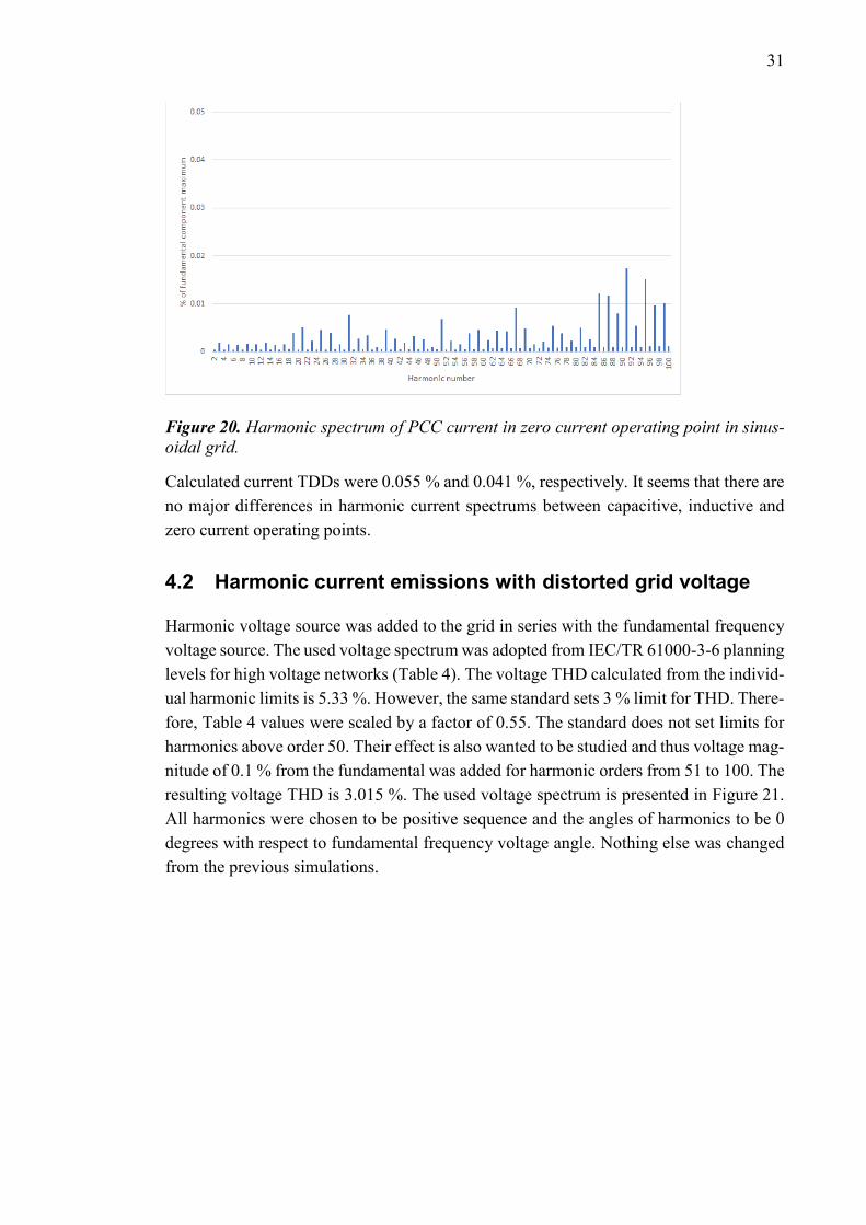
31

Figure 20. Harmonic spectrum of PCC current in zero current operating point in sinus-

oidal grid.

Calculated current TDDs were 0.055 % and 0.041 %, respectively. It seems that there are

no major differences in harmonic current spectrums between capacitive, inductive and

zero current operating points.

4.2 Harmonic current emissions with distorted grid voltage

Harmonic voltage source was added to the grid in series with the fundamental frequency

voltage source. The used voltage spectrum was adopted from IEC/TR 61000-3-6 planning

levels for high voltage networks (Table 4). The voltage THD calculated from the individ-

ual harmonic limits is 5.33 %. However, the same standard sets 3 % limit for THD. There-

fore, Table 4 values were scaled by a factor of 0.55. The standard does not set limits for

harmonics above order 50. Their effect is also wanted to be studied and thus voltage mag-

nitude of 0.1 % from the fundamental was added for harmonic orders from 51 to 100. The

resulting voltage THD is 3.015 %. The used voltage spectrum is presented in Figure 21.

All harmonics were chosen to be positive sequence and the angles of harmonics to be 0

degrees with respect to fundamental frequency voltage angle. Nothing else was changed

from the previous simulations.

32

Figure 21. Grid’s harmonic voltage spectrum used in the simulations.

Simulations were done with the harmonic voltage source. They were done with both sec-

ondary busbar voltage feedforward options and in the same three operating points as with

sinusoidal grid voltage. First, fundamental voltage feedforward was used. Simulated har-

monic spectrum of PCC current in capacitive operating point is shown in Figure 22.

Figure 22. Harmonic spectrum of PCC current in capacitive operating point in distorted

grid with fundamental voltage feedforward.

Calculated current TDD was 0.790 % when all 100 harmonic components were consid-

ered. It is almost 21 times the simulated current TDD with sinusoidal grid voltage. Clear

correlation between voltage and current harmonic spectrums can be seen. In other words,

at those harmonics where largest voltages were introduced, current increased the most.

Comparable PCC harmonic current spectrums in inductive and zero current operating

points are shown in Figure 23 and Figure 24.

33

Figure 23. Harmonic spectrum of PCC current in inductive operating point in distorted

grid with fundamental voltage feedforward.

Figure 24. Harmonic spectrum of PCC current in zero current operating point in dis-

torted grid with fundamental voltage feedforward.

Calculated current TDDs were 0.820 % and 0.792 %, respectively. The current spectrums

of simulated cases are very similar and they all show that if magnitude of harmonic volt-

age order h is increased also the magnitude of same order harmonic current increases.

Simulated harmonic spectrums with instantaneous voltage feedforward differ from the

fundamental voltage feedforward results. Spectrums in capacitive, inductive and zero cur-

rent operating points are presented in Figure 25, Figure 26 and Figure 27.

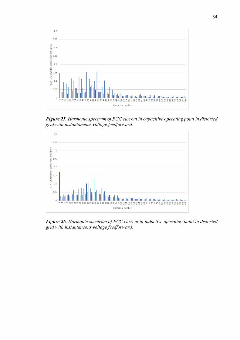
34

Figure 25. Harmonic spectrum of PCC current in capacitive operating point in distorted

grid with instantaneous voltage feedforward.

Figure 26. Harmonic spectrum of PCC current in inductive operating point in distorted

grid with instantaneous voltage feedforward.

35

Figure 27. Harmonic spectrum of PCC current in zero current operating point in dis-

torted grid with instantaneous voltage feedforward.

Calculated current TDDs were 0.496 %, 0.401 % and 0.346 %. They are 7 - 13 times the

respective current TDDs with sinusoidal voltage. TDDs and low-order harmonics are yet

lower than with fundamental voltage feedforward. Harmonic currents of orders from 20

to 40 are however larger. With fundamental voltage feedforward current spectrum resem-

bled the grid voltage spectrum. Now current spectrums are not so predictable any more.

4.3 Effect of harmonic currents on PCC voltage in inductive

grid

The harmonic spectrum of PCC current in capacitive operating point with fundamental

voltage feedforward was shown in Figure 22. Compared to IEEE 519 harmonic current

distortion limits (Table 2), the produced harmonic currents are still small and not a prob-

lem with respect to that. However, harmonic currents flowing through the grid imped-

ances affect harmonic voltages at PCC as explained in chapter 2.1. As voltage THD in

grid was already at the limit of IEC/TR 61000-3-6 standard, STATCOM produced har-

monic currents should not increase the voltage distortion at PCC. Simulated grid and PCC

voltage spectrums in capacitive operating point with fundamental voltage feedforward

are presented in Figure 28 and Figure 29. Harmonic voltages are expressed as percent of

nominal fundamental frequency line-to-neutral voltage which is 138/√3 kV.

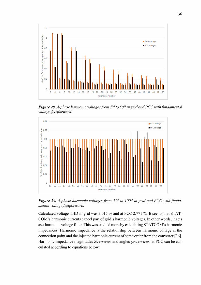
36

Figure 28. A-phase harmonic voltages from 2nd to 50th in grid and PCC with fundamental

voltage feedforward.

Figure 29. A-phase harmonic voltages from 51st to 100th in grid and PCC with funda-

mental voltage feedforward.

Calculated voltage THD in grid was 3.015 % and at PCC 2.771 %. It seems that STAT-

COM’s harmonic currents cancel part of grid’s harmonic voltages. In other words, it acts

as a harmonic voltage filter. This was studied more by calculating STATCOM’s harmonic

impedances. Harmonic impedance is the relationship between harmonic voltage at the

connection point and the injected harmonic current of same order from the converter [36].

Harmonic impedance magnitudes Zh,STATCOM and angles φZ,h,STATCOM at PCC can be cal-

culated according to equations below:

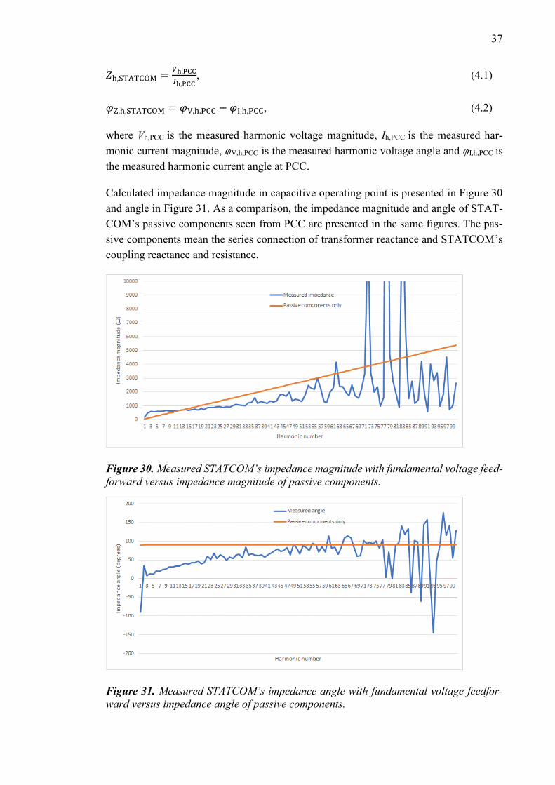
37

𝑍h,STATCOM =𝑉h,PCC

𝐼h,PCC, (4.1)

𝜑Z,h,STATCOM = 𝜑V,h,PCC − 𝜑I,h,PCC, (4.2)

where Vh,PCC is the measured harmonic voltage magnitude, Ih,PCC is the measured har-

monic current magnitude, φV,h,PCC is the measured harmonic voltage angle and φI,h,PCC is

the measured harmonic current angle at PCC.

Calculated impedance magnitude in capacitive operating point is presented in Figure 30

and angle in Figure 31. As a comparison, the impedance magnitude and angle of STAT-

COM’s passive components seen from PCC are presented in the same figures. The pas-

sive components mean the series connection of transformer reactance and STATCOM’s

coupling reactance and resistance.

Figure 30. Measured STATCOM’s impedance magnitude with fundamental voltage feed-

forward versus impedance magnitude of passive components.

Figure 31. Measured STATCOM’s impedance angle with fundamental voltage feedfor-

ward versus impedance angle of passive components.

38

At most frequencies STATCOM’s impedance is inductive-resistive (angle positive) and

at those frequencies harmonic voltages at PCC mitigate. Some harmonic impedances

(86th, 89th and 93rd) are capacitive-resistive (angle negative) and at those frequencies har-

monic voltages increase at PCC. Fundamental component of impedance is almost capac-

itive as expected in capacitive operating point.

The reason for previous phenomenon can be found from Kirchoff’s voltage law and

phasor diagram for the harmonic component. According to the voltage law, voltage of the

simulated circuit can be presented as

𝑉h,grid = 𝑉h,PCC + 𝑍h,grid𝐼h,STATCOM, (4.3)

where 𝑉h,grid is the harmonic voltage in grid, 𝑉h,PCC is the harmonic voltage at PCC,𝑍h,grid

is the grid’s harmonic impedance and 𝐼h,STATCOM is the produced harmonic current of

STATCOM. According to the equation a phasor diagram can be drawn. In Figure 32

phasor diagrams are drawn in two situations. In the first situation, the harmonic current

of STATCOM is inductive-resistive (current lags voltage) and in the second it is capaci-

tive-resistive (current leads voltage). Grid impedance is simplified to have only inductive

reactance component jXh,grid, because in the simulations reactance was about 10 times

larger than resistance at fundamental frequency. As the inductive reactance increases as

function of frequency, the ratio between reactance and resistance is even larger at har-

monics.

Figure 32. Phasor diagram of grid’s and PCC’s harmonic voltages in inductive grid,

when STATCOM’s harmonic current is a) inductive-resistive, b) capacitive-resistive.

The voltage drop in grid impedance causes difference between grid’s and PCC’s har-

monic voltage amplitudes. When STATCOM’s harmonic current is inductive-resistive,

harmonic voltage amplitude at PCC is smaller than the harmonic voltage amplitude in

grid. When the current is capacitive-resistive, situation is the opposite.

It seems that if fundamental voltage feedforward is used, harmonic voltage at PCC sees

STATCOM as inductive-resistive impedance at harmonics up to 70th order. This causes

inductive-resistive current and smaller PCC voltage at those harmonics. The measured

impedance resembles the calculated passive component impedance to some extent but

there is also deviation between them. At least at lower frequencies, measured resistance

Vh,PCC

Ih,STATCOM

jXh,gridIh,STATCOM

Vh,grid

a) b)

Ih,STATCOM

Vh,PCC

jXh,gridIh,STATCOMVh,grid

39

is clearly larger than calculated. This deviation implies that the total impedance is affected

also by the produced STATCOM voltage. Thus, changing STATCOM’s voltage output

by the means of control and modulation can lead to higher impedance and lower harmonic

current emissions. Ideally, converter’s harmonic impedance would be infinite which

would mean zero harmonic currents independent of grid harmonic voltages [36].

The situation changes if instantaneous voltage feedforward is used. The harmonic current

spectrum in capacitive operating point was presented in Figure 25. In this operating point,

harmonic voltage spectrums in grid and PCC are presented in Figure 33 and Figure 34.

Figure 33. A-phase harmonic voltages from 2nd to 50th in grid and PCC with instantane-

ous voltage feedforward.

Figure 34. A-phase harmonic voltages from 51st to 100th in grid and PCC with instanta-

neous voltage feedforward.

40

Voltage THD at PCC was now 3.034 % which is higher than THD of grid voltage. Even

though the total amount of harmonic current emissions is smaller than with fundamental

voltage feedforward, these harmonic currents produce harmonic voltages at grid imped-

ances so that many of the PCC harmonic voltages increase. Again, STATCOM’s har-

monic impedances were calculated from measured PCC voltage and current. Impedance

magnitude is presented in Figure 35 and angle in Figure 36.

Figure 35. STATCOM’s impedance magnitude measured at PCC with instantaneous volt-

age feedforward.

Figure 36. STATCOM’s impedance angle measured at PCC with instantaneous voltage

feedforward.

Now STATCOM’s impedance is capacitive-resistive also at many low-order harmonics.

This means that STATCOM produces capacitive-resistive current at those frequencies

which cause harmonic voltages at PCC to rise compared to the grid harmonic voltages.

The idea of instantaneous voltage feedforward is to remove the effect of grid harmonic

voltages on produced harmonic currents by adding an additional voltage term to the cur-

rent controller output [37]. In case of inverter connected to the grid through an LCL-filter,

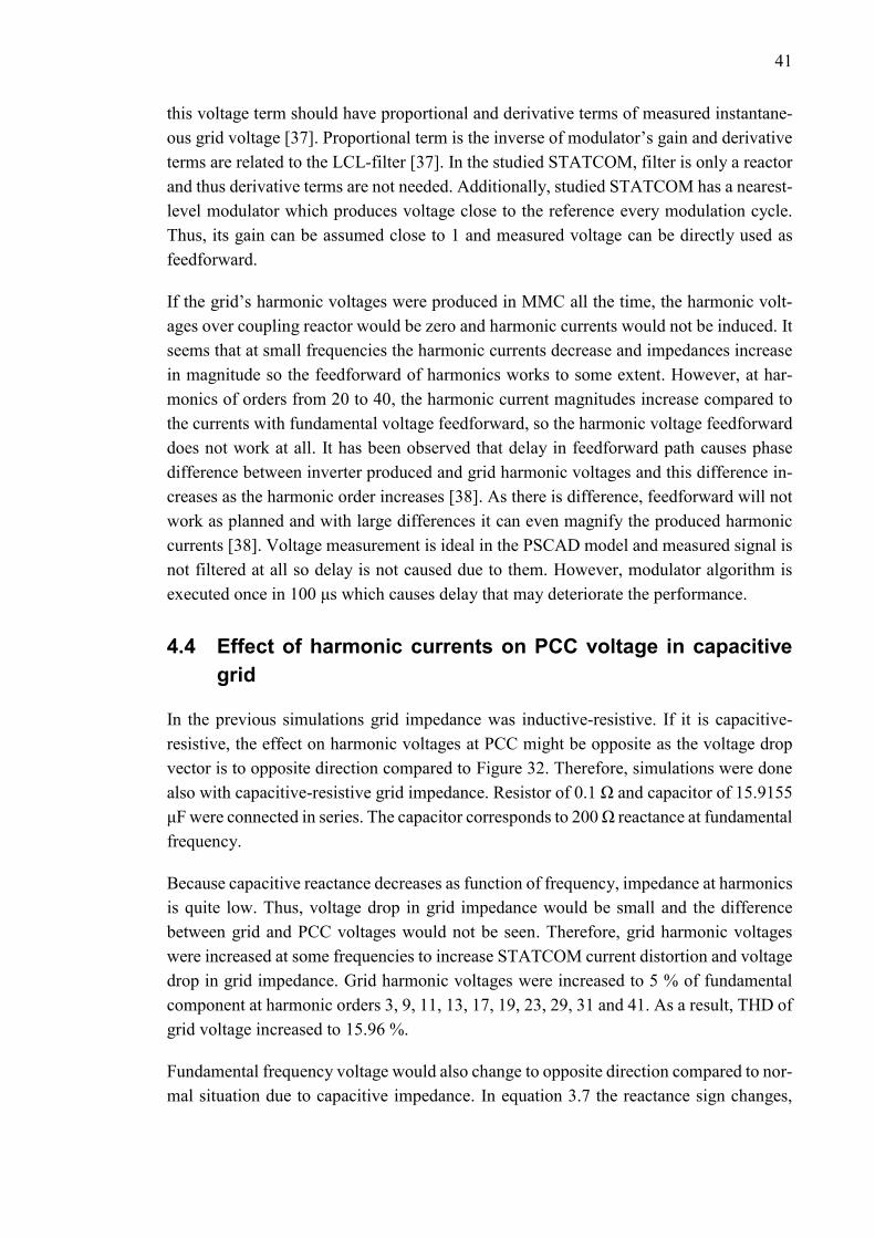
41

this voltage term should have proportional and derivative terms of measured instantane-

ous grid voltage [37]. Proportional term is the inverse of modulator’s gain and derivative

terms are related to the LCL-filter [37]. In the studied STATCOM, filter is only a reactor

and thus derivative terms are not needed. Additionally, studied STATCOM has a nearest-

level modulator which produces voltage close to the reference every modulation cycle.

Thus, its gain can be assumed close to 1 and measured voltage can be directly used as

feedforward.

If the grid’s harmonic voltages were produced in MMC all the time, the harmonic volt-

ages over coupling reactor would be zero and harmonic currents would not be induced. It

seems that at small frequencies the harmonic currents decrease and impedances increase

in magnitude so the feedforward of harmonics works to some extent. However, at har-

monics of orders from 20 to 40, the harmonic current magnitudes increase compared to

the currents with fundamental voltage feedforward, so the harmonic voltage feedforward

does not work at all. It has been observed that delay in feedforward path causes phase

difference between inverter produced and grid harmonic voltages and this difference in-

creases as the harmonic order increases [38]. As there is difference, feedforward will not

work as planned and with large differences it can even magnify the produced harmonic

currents [38]. Voltage measurement is ideal in the PSCAD model and measured signal is

not filtered at all so delay is not caused due to them. However, modulator algorithm is

executed once in 100 μs which causes delay that may deteriorate the performance.

4.4 Effect of harmonic currents on PCC voltage in capacitive

grid

In the previous simulations grid impedance was inductive-resistive. If it is capacitive-

resistive, the effect on harmonic voltages at PCC might be opposite as the voltage drop

vector is to opposite direction compared to Figure 32. Therefore, simulations were done

also with capacitive-resistive grid impedance. Resistor of 0.1 Ω and capacitor of 15.9155

μF were connected in series. The capacitor corresponds to 200 Ω reactance at fundamental

frequency.

Because capacitive reactance decreases as function of frequency, impedance at harmonics

is quite low. Thus, voltage drop in grid impedance would be small and the difference

between grid and PCC voltages would not be seen. Therefore, grid harmonic voltages

were increased at some frequencies to increase STATCOM current distortion and voltage

drop in grid impedance. Grid harmonic voltages were increased to 5 % of fundamental

component at harmonic orders 3, 9, 11, 13, 17, 19, 23, 29, 31 and 41. As a result, THD of

grid voltage increased to 15.96 %.

Fundamental frequency voltage would also change to opposite direction compared to nor-

mal situation due to capacitive impedance. In equation 3.7 the reactance sign changes,

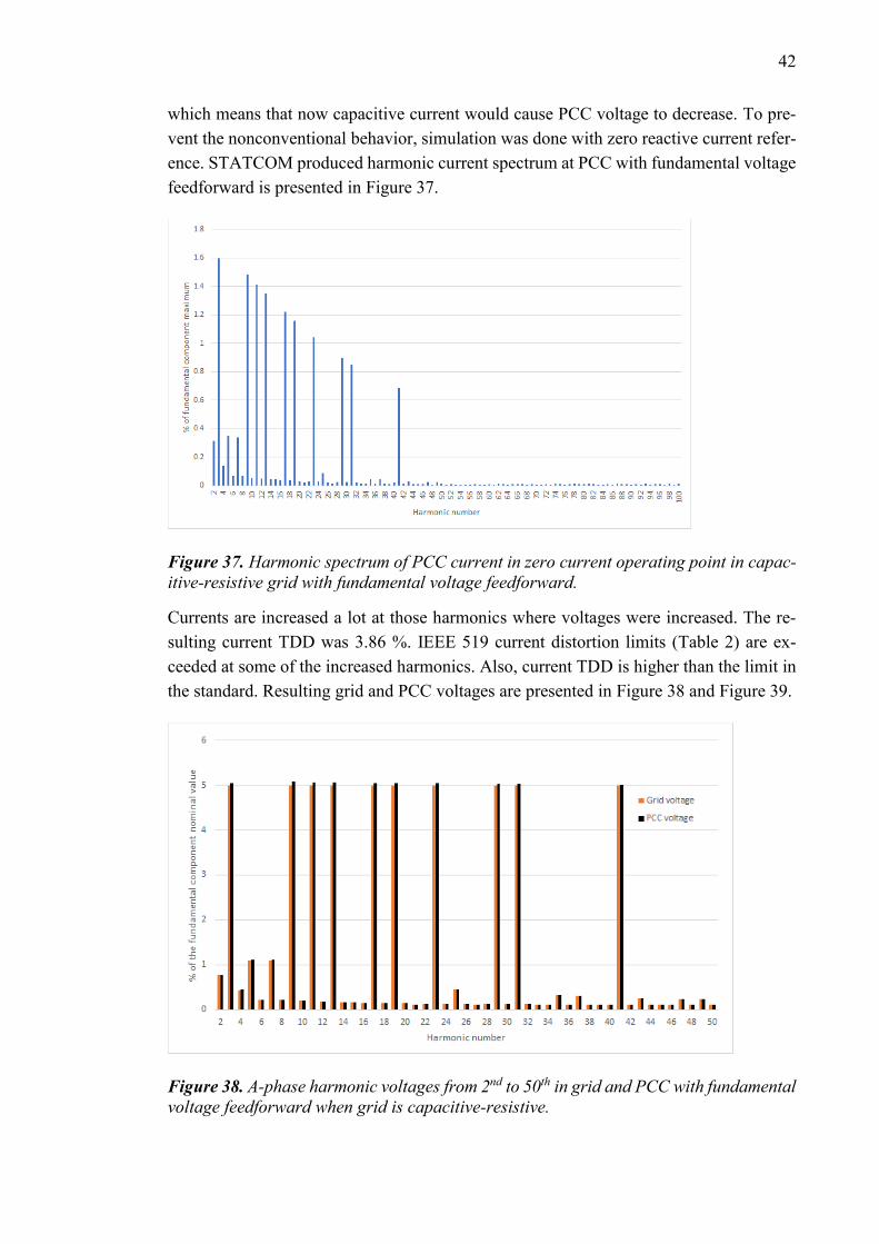
42

which means that now capacitive current would cause PCC voltage to decrease. To pre-

vent the nonconventional behavior, simulation was done with zero reactive current refer-

ence. STATCOM produced harmonic current spectrum at PCC with fundamental voltage

feedforward is presented in Figure 37.

Figure 37. Harmonic spectrum of PCC current in zero current operating point in capac-

itive-resistive grid with fundamental voltage feedforward.

Currents are increased a lot at those harmonics where voltages were increased. The re-

sulting current TDD was 3.86 %. IEEE 519 current distortion limits (Table 2) are ex-

ceeded at some of the increased harmonics. Also, current TDD is higher than the limit in

the standard. Resulting grid and PCC voltages are presented in Figure 38 and Figure 39.

Figure 38. A-phase harmonic voltages from 2nd to 50th in grid and PCC with fundamental

voltage feedforward when grid is capacitive-resistive.

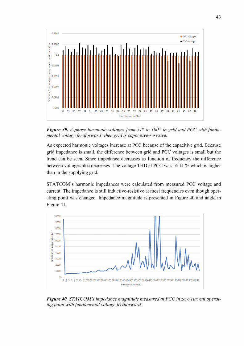
43

Figure 39. A-phase harmonic voltages from 51st to 100th in grid and PCC with funda-

mental voltage feedforward when grid is capacitive-resistive.

As expected harmonic voltages increase at PCC because of the capacitive grid. Because

grid impedance is small, the difference between grid and PCC voltages is small but the

trend can be seen. Since impedance decreases as function of frequency the difference

between voltages also decreases. The voltage THD at PCC was 16.11 % which is higher

than in the supplying grid.

STATCOM’s harmonic impedances were calculated from measured PCC voltage and

current. The impedance is still inductive-resistive at most frequencies even though oper-

ating point was changed. Impedance magnitude is presented in Figure 40 and angle in

Figure 41.

Figure 40. STATCOM’s impedance magnitude measured at PCC in zero current operat-

ing point with fundamental voltage feedforward.

44

Figure 41. STATCOM’s impedance angle measured at PCC in zero current operating

point with fundamental voltage feedforward.

Phasor diagrams were drawn according to the equation 4.3 assuming capacitive grid im-

pedance. In the first diagram STATCOM produced harmonic current is inductive-resis-

tive and in the second diagram it is capacitive-resistive. The diagrams are presented in

Figure 42.

Figure 42. Phasor diagram of grid and PCC harmonic voltages in capacitive grid, when

STATCOM’s harmonic current is a) inductive-resistive, b) capacitive-resistive.

The situation is now opposite compared to inductive grid. When STATCOM’s current is

inductive-resistive, the voltage drop in capacitive grid impedance -jXh,grid causes larger

harmonic voltage magnitude at PCC than in the supplying grid. When the current is ca-

pacitive-resistive, PCC harmonic voltage magnitude is smaller than the voltage magni-

tude in grid.

Simulation with same parameters was done also with instantaneous voltage feedforward.

Harmonic current spectrum at PCC is presented in Figure 43.

Vh,PCC

Ih,STATCOM

-jXh,gridIh,STATCOM

Vh,grid

a) b)

Ih,STATCOM

Vh,PCC

-jXh,gridIh,STATCOM

Vh,grid

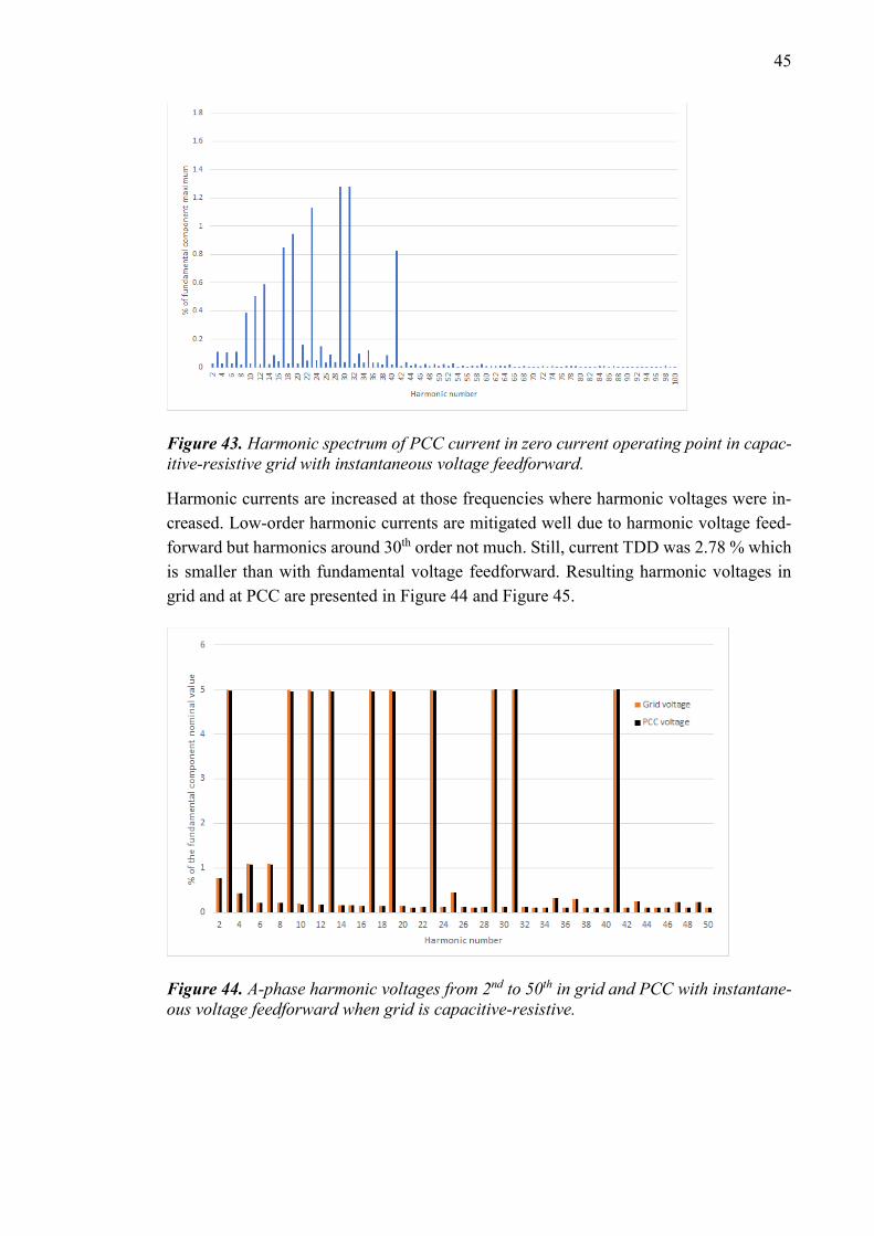
45

Figure 43. Harmonic spectrum of PCC current in zero current operating point in capac-

itive-resistive grid with instantaneous voltage feedforward.

Harmonic currents are increased at those frequencies where harmonic voltages were in-

creased. Low-order harmonic currents are mitigated well due to harmonic voltage feed-

forward but harmonics around 30th order not much. Still, current TDD was 2.78 % which

is smaller than with fundamental voltage feedforward. Resulting harmonic voltages in

grid and at PCC are presented in Figure 44 and Figure 45.

Figure 44. A-phase harmonic voltages from 2nd to 50th in grid and PCC with instantane-

ous voltage feedforward when grid is capacitive-resistive.

46

Figure 45. A-phase harmonic voltages from 51st to 100th in grid and PCC with instanta-

neous voltage feedforward when grid is capacitive-resistive.

Low-order harmonic voltages are decreased a bit at PCC but 29th, 31st and 41st harmonics

are increased compared to grid. The reason can be found from STATCOM’s impedance

measured at PCC whose magnitude is shown in Figure 46 and angle in Figure 47.

Figure 46. STATCOM’s impedance magnitude measured at PCC in zero current operat-

ing point with instantaneous voltage feedforward.

47

Figure 47. STATCOM’s impedance angle measured at PCC in zero current operating

point with instantaneous voltage feedforward.

It seems that STATCOM’s impedance decreases up to 30th harmonic and starts to increase

after that. It explains that the highest harmonic currents are around the 30th harmonic. The

impedance also changes quite randomly between inductive-resistive and capacitive-resis-

tive which explains that at some frequencies harmonic voltages increase at PCC and at

some frequencies they decrease.

4.5 Comparison of voltage feedforward options

Based on the simulation results presented in the earlier subchapters voltage feedforward

options were compared. When instantaneous value of measured secondary busbar voltage

with all the harmonics is used as feedforward, STATCOM’s impedance is quite high at

low-order harmonics. However, the impedance seems to have a dip around 30th harmonic.

That means relatively high harmonic current emissions at those frequencies if there are

harmonic voltages present. High currents at high-order harmonics cause large harmonic

voltage drops in inductive grid where impedance increases as function of frequency. The

impedance angle is also very unpredictable so it can not be predicted if the harmonic

voltage drop causes PCC harmonic voltage to rise or decrease even if grid impedance was

known. Moreover, measuring harmonic voltages might be inaccurate which would dete-

riorate the performance and cause unpredictability even more.

When fundamental component of secondary busbar voltage is used as feedforward,

STATCOM’s impedance is quite predictable. It seems to be inductive-resistive at least

up to 70th harmonic and increases as function of frequency. Impedance is lowest at low-

order harmonics and thus highest harmonic currents appear at those frequencies. How-

ever, low-order harmonic currents can be mitigated by means of current control which is

shown in chapter 5.2. The impedance around 30th harmonic is higher than with instanta-

neous feedforward so the high-order harmonic currents are mitigated more efficiently. On

the other hand, if harmonic voltage feedforward was used for low-order harmonics only,

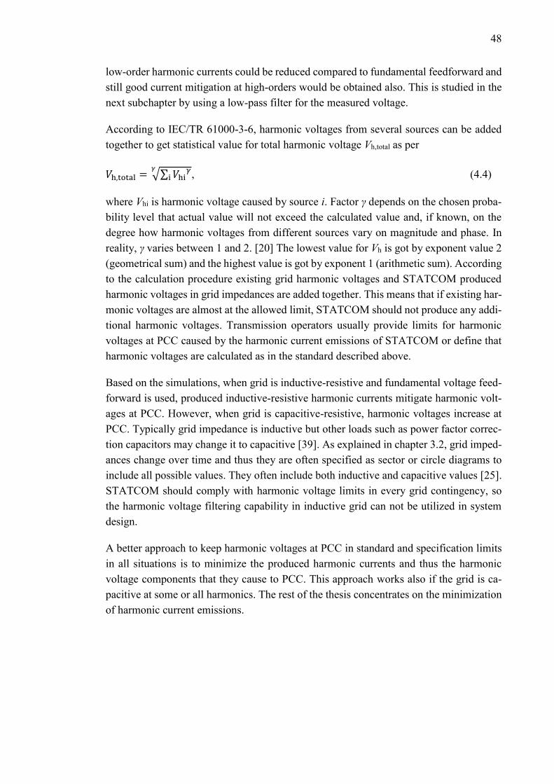
48

low-order harmonic currents could be reduced compared to fundamental feedforward and

still good current mitigation at high-orders would be obtained also. This is studied in the

next subchapter by using a low-pass filter for the measured voltage.

According to IEC/TR 61000-3-6, harmonic voltages from several sources can be added

together to get statistical value for total harmonic voltage Vh,total as per

𝑉h,total = √∑ 𝑉hi𝛾

i𝛾

, (4.4)

where Vhi is harmonic voltage caused by source i. Factor γ depends on the chosen proba-

bility level that actual value will not exceed the calculated value and, if known, on the

degree how harmonic voltages from different sources vary on magnitude and phase. In

reality, γ varies between 1 and 2. [20] The lowest value for Vh is got by exponent value 2

(geometrical sum) and the highest value is got by exponent 1 (arithmetic sum). According

to the calculation procedure existing grid harmonic voltages and STATCOM produced

harmonic voltages in grid impedances are added together. This means that if existing har-

monic voltages are almost at the allowed limit, STATCOM should not produce any addi-

tional harmonic voltages. Transmission operators usually provide limits for harmonic

voltages at PCC caused by the harmonic current emissions of STATCOM or define that

harmonic voltages are calculated as in the standard described above.

Based on the simulations, when grid is inductive-resistive and fundamental voltage feed-

forward is used, produced inductive-resistive harmonic currents mitigate harmonic volt-

ages at PCC. However, when grid is capacitive-resistive, harmonic voltages increase at

PCC. Typically grid impedance is inductive but other loads such as power factor correc-

tion capacitors may change it to capacitive [39]. As explained in chapter 3.2, grid imped-

ances change over time and thus they are often specified as sector or circle diagrams to

include all possible values. They often include both inductive and capacitive values [25].

STATCOM should comply with harmonic voltage limits in every grid contingency, so

the harmonic voltage filtering capability in inductive grid can not be utilized in system

design.

A better approach to keep harmonic voltages at PCC in standard and specification limits

in all situations is to minimize the produced harmonic currents and thus the harmonic

voltage components that they cause to PCC. This approach works also if the grid is ca-

pacitive at some or all harmonics. The rest of the thesis concentrates on the minimization

of harmonic current emissions.

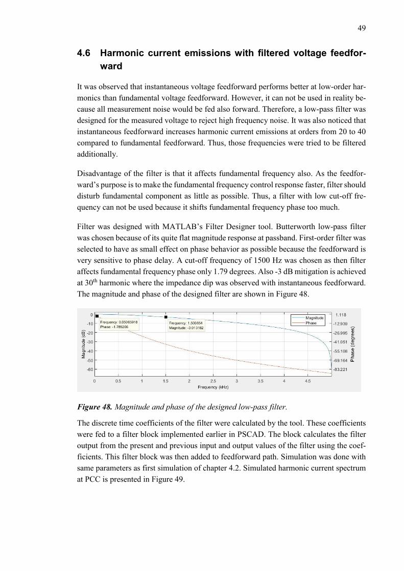
49

4.6 Harmonic current emissions with filtered voltage feedfor-

ward

It was observed that instantaneous voltage feedforward performs better at low-order har-

monics than fundamental voltage feedforward. However, it can not be used in reality be-

cause all measurement noise would be fed also forward. Therefore, a low-pass filter was

designed for the measured voltage to reject high frequency noise. It was also noticed that

instantaneous feedforward increases harmonic current emissions at orders from 20 to 40

compared to fundamental feedforward. Thus, those frequencies were tried to be filtered

additionally.

Disadvantage of the filter is that it affects fundamental frequency also. As the feedfor-

ward’s purpose is to make the fundamental frequency control response faster, filter should

disturb fundamental component as little as possible. Thus, a filter with low cut-off fre-

quency can not be used because it shifts fundamental frequency phase too much.

Filter was designed with MATLAB’s Filter Designer tool. Butterworth low-pass filter

was chosen because of its quite flat magnitude response at passband. First-order filter was

selected to have as small effect on phase behavior as possible because the feedforward is

very sensitive to phase delay. A cut-off frequency of 1500 Hz was chosen as then filter

affects fundamental frequency phase only 1.79 degrees. Also -3 dB mitigation is achieved

at 30th harmonic where the impedance dip was observed with instantaneous feedforward.

The magnitude and phase of the designed filter are shown in Figure 48.

Figure 48. Magnitude and phase of the designed low-pass filter.

The discrete time coefficients of the filter were calculated by the tool. These coefficients

were fed to a filter block implemented earlier in PSCAD. The block calculates the filter

output from the present and previous input and output values of the filter using the coef-

ficients. This filter block was then added to feedforward path. Simulation was done with

same parameters as first simulation of chapter 4.2. Simulated harmonic current spectrum

at PCC is presented in Figure 49.

50

Figure 49. Harmonic spectrum of PCC current in capacitive operating point with low-

pass filtered voltage feedforward.

Calculated current TDD was 0.589 % which is larger than with instantaneous voltage

feedforward but clearly smaller than with fundamental voltage feedforward. Low-order

harmonics are quite well mitigated but not as well as with instantaneous feedforward. The

phase delay of the filter deteriorates the harmonic performance when the frequency in-

creases. Due to delay, harmonic currents of orders from 10 to 20 have increased substan-

tially compared to instantaneous feedforward. However, at high frequencies the magni-

tude of the filter decreases and thus the feedforward effect decreases. That is desirable

because at harmonics around 30th order instantaneous feedforward effect was negative as

it increased harmonics compared to fundamental feedforward. Now, harmonics around

30th order are considerably smaller than with instantaneous feedforward. Still, accurate

harmonic voltage measurement in filter’s passband is needed to achieve this performance.

STATCOM’s impedance magnitude with filtered voltage feedforward is presented in Fig-

ure 50 and angle in Figure 51. Impedance magnitude has increased at low-orders com-

pared to fundamental feedforward and around 30th order compared to instantaneous feed-

forward. However, it has decreased at low-order harmonics up to 20th order in comparison

with instantaneous feedforward. Impedances are capacitive at low-order harmonics so in

inductive grid they would cause increased harmonic voltages to PCC.

51

Figure 50. STATCOM’s impedance magnitude measured at PCC in capacitive operating

point with low-pass filtered voltage feedforward.

Figure 51. STATCOM’s impedance angle measured at PCC in capacitive operating point

with low-pass filtered voltage feedforward.

4.7 Harmonic current emissions with increased reactance

Harmonic current emissions can be decreased by increasing the impedance of STAT-

COM. The effect of increasing the impedance of STATCOM’s passive components is

studied in this chapter. First, transformer’s reactance was increased by 50 % to 0.1725

p.u. Other parameters were same as in the first simulation of chapter 4.2. The harmonic

spectrum of current measured at PCC is shown in Figure 52.

52

Figure 52. Harmonic spectrum of PCC current with higher transformer’s reactance.

Compared to Figure 22, harmonic currents have decreased only slightly. Calculated cur-

rent TDD was 0.749 % which is only a bit lower than with original reactance value.

Next, transformer’s reactance was changed back to its original value and coupling reac-

tor’s inductance was increased by 50 % to 16.5 mH. Other parameters were not changed.

The harmonic spectrum of current measured at PCC is presented in Figure 53.

Figure 53. Harmonic spectrum of PCC current with higher coupling reactor’s induct-

ance.

Calculated current TDD was 0.758 %. Harmonic currents have decreased only a little.

However, as inductance is increased, changing speed of STATCOM’s output current is

slowed down as equation for inductor shows:

53

𝑑𝑖L

𝑑𝑡=

𝑣L

𝐿, (4.5)

where iL is inductor current, vL inductor voltage and L inductance. The increase of induct-

ance can be compensated by increasing the P-gain (proportional gain) of current control-

ler also by 50 %. That causes 50 % higher voltage component over inductor for same

error between current reference and measured current and thus results in same current

changing speed. Therefore, same dynamic performance is achieved as with original reac-

tor and lower P-gain. The simulated harmonic spectrum of PCC current with increased P-

gain and reactance is presented in Figure 54.

Figure 54. Harmonic spectrum of PCC current with higher coupling reactor’s inductance

and P-gain.

Calculated current TDD was 0.571 % so the increase of both factors reduces harmonic

currents considerably. The increase of reactor’s inductance is not an effective way to de-

crease harmonic currents itself but when it is combined with increase of P-gain, effect is

significant.

The disadvantage of increasing the reactance of the components is that more material is

needed and thus costs are increased. Moreover, as reactance is increased, higher converter

voltage is needed to produce same capacitive current as equation 3.18 states. To produce

higher converter voltage more submodules are needed in series which also raises costs.

Increasing current controller’s P-gain without changing any component values was stud-

ied for voltage-source converter connected to grid through an LCL-filter [36]. It was ob-

served that increase of P-gain decreases harmonic currents but makes the converter cur-

rent more oscillatory in transient situations [36]. That would happen for STATCOM too

because higher P-gain causes higher voltage reference and thus higher voltage over cou-

pling reactor for same current error. According to equation 4.5, that increases the current

changing speed.

54

5. SOURCES OF HARMONIC CURRENTS

In the earlier chapter secondary busbar voltage feedforward options were compared. Ad-

vantages of fundamental voltage feedforward were quite predictable behavior of STAT-

COM’s impedance, good mitigation of high-order harmonic currents and no need for har-

monic voltage measurement which might be inaccurate. Disadvantages were higher har-

monic currents at low frequencies. However, it is shown in this chapter that at least in

simulations with ideal current measurement they can be controlled to very small values

by means of current control. Advantage of instantaneous voltage feedforward was better

mitigation of low-order harmonic currents. However, harmonic currents of orders from

20 to 40 were larger than with fundamental feedforward. In addition, exact harmonic

voltage measurement is required. Low-pass filtered voltage feedforward combined the

good mitigation of low-order harmonics and harmonics around 30th order but increased

harmonic currents of orders from 10 to 20. Effect of harmonic currents on PCC harmonic

voltages was studied but it was concluded that this information can not be utilized as the

effect depends on grid impedance which changes over time. It was also shown that har-

monic currents could be decreased by increasing the coupling reactor’s reactance. Its ef-

fect is small itself but when combined with increased current controller’s P-gain the har-

monics could be decreased considerably. The disadvantage is that more reactor material

and converter submodules are needed and therefore costs increase.

In this chapter, it is investigated if modulator or different controllers have effect on STAT-

COM’s harmonic current emissions. Simulations are done where modulator or control

block is made ideal and the produced harmonic current spectrum is compared to the spec-

trum of reference case. The reference case is the first simulation in chapter 4.2 whose

current spectrum is shown in Figure 22. Moreover, solutions to decrease harmonics in the

viewpoint of each control function are proposed or developed. First, the effect of modu-

lator is investigated. Then, current controller and DC-link voltage controller impacts are

studied. Last, manual current q-component control is changed to voltage control and the

changes in harmonic spectrum are investigated. Synchronization to secondary busbar

voltage is simplified in this simulation model so its effect is not studied. In this model it

is implemented as Fast Fourier Transform which extracts the phase angles of secondary

busbar’s fundamental frequency line-to-line voltages.

5.1 Modulator effect

An ideal modulator produces exactly the reference voltage. It also balances submodule

voltages so well that their voltages stay constant. That is impossible in a real system but

this way additional harmonic voltages that are caused by the operation of modulator can

55

be eliminated. Still, produced voltage is not necessarily sinusoidal because reference volt-

age may contain harmonic components. It is investigated if producing the exact reference

voltage decreases harmonic currents of STATCOM. In that case, other modulator

schemes could be considered to improve performance.

Ideal modulator was implemented by setting the output voltage of converter equal to ref-

erence voltage. Submodule voltages were forced to stay at their nominal value. Figure 55

presents simulated harmonic current spectrum measured from PCC when ideal modulator

was used and other parameters were same as in the reference case.

Figure 55. Harmonic spectrum of PCC current with ideal modulator.

Calculated current TDD was 0.774 % which is slightly lower than with original modula-

tor. Harmonic currents are not decreased much but they are more predictable. It seems

that if there are equal voltage magnitudes at some harmonics in grid, the magnitudes of

those harmonic currents decrease linearly as function of frequency. The effect can be seen

at harmonics from 51st to 100th where grid harmonic voltages are equal magnitude (0.1 %

of the fundamental). Produced harmonic currents decrease quite linearly as function of

frequency because the inductive reactances of passive components increase. When the

original modulator was used, these higher frequency harmonics were more unpredictable.

Another example are the harmonics 3, 5 and 7 which also have equal magnitudes in grid

voltage but the current magnitudes decrease linearly when the frequency increases.

Next, harmonic current emissions were simulated using the ideal modulator with sinus-

oidal grid voltage. The harmonic spectrum of current at PCC is shown in Figure 56.

56

Figure 56. Harmonic spectrum of PCC current with ideal modulator and sinusoidal grid

voltage.

Calculated current TDD was only 0.00004 %. It seems that when grid voltage is sinusoi-

dal, modulator causes all the harmonic current emissions. However, the emissions are

already very low with original modulator in that situation (Figure 18) and not usually a

problem.

The original modulator is a modification of nearest-level control modulation scheme. In

this kind of modulator, the spectrum of voltage is spread to all harmonics [34]. If grid

voltage is sinusoidal, those harmonic components appear in current also. In some other

modulator schemes harmonic voltages could be centered to higher frequencies. In phase-

shifted carrier modulation the lowest order harmonics would appear at the sidebands of

the harmonic whose order is the number of submodules in one phase multiplied by the

ratio of carrier frequency to fundamental frequency [34]. If the number of submodules is

high enough, low-order harmonics are decreased a lot [34]. Same voltage waveform and

thus harmonics could also be achieved with level-shifted carrier modulation having an

alternative phase opposition disposition between adjacent two levels [34]. This could be

beneficial if producing currents at some low-order harmonics is forbidden and grid volt-

age does not have those harmonic components. As observed in Figure 55 for ideal mod-

ulator, if there are harmonic voltages in grid voltage, also harmonic currents of same or-

ders appear so the modulator scheme does not really make a difference.

In the earlier chapter, it was concluded that the instantaneous voltage feedforward does

not work as it is planned to. Now, simulation was done to see if using ideal modulator

without delays would improve the harmonic performance when instantaneous feedfor-

ward is used. Grid’s harmonic voltages were set back to reference case values. The har-

monic spectrum of current measured at PCC is shown in Figure 57.

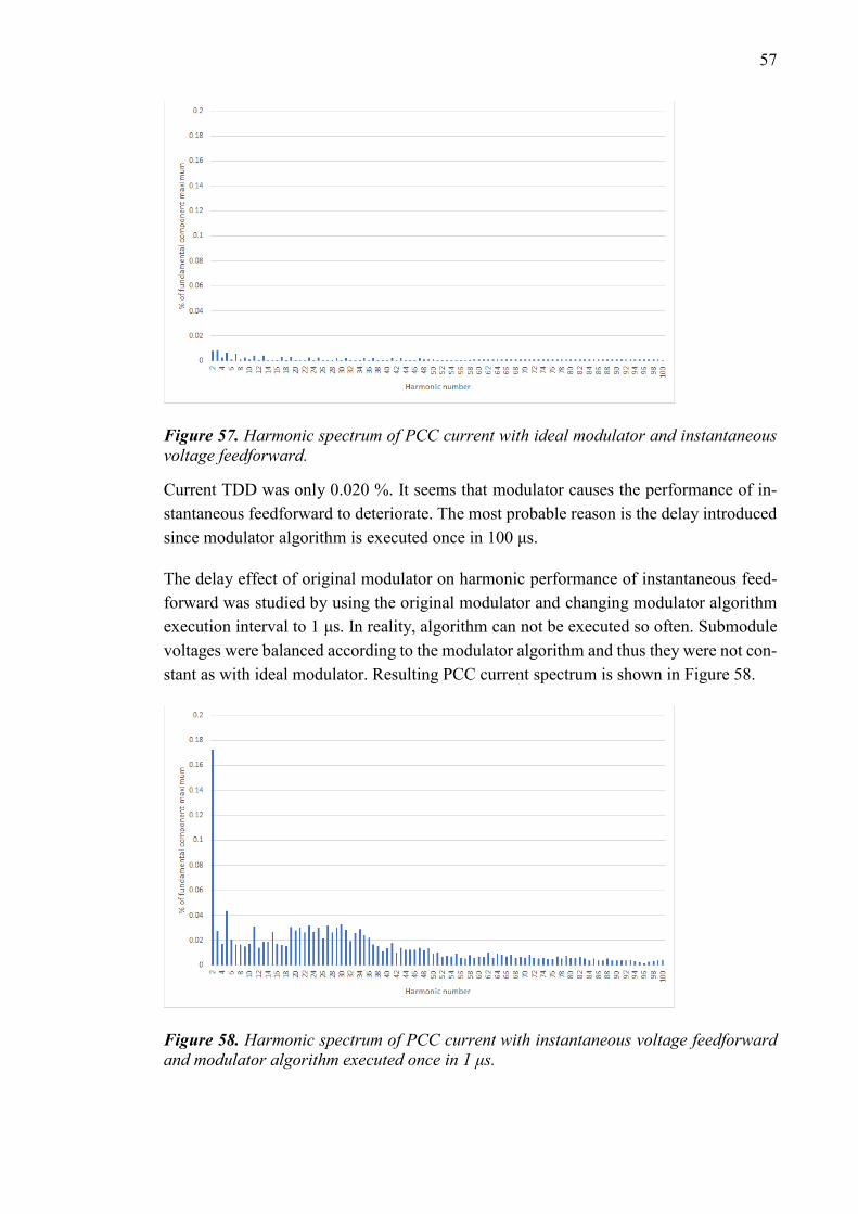
57

Figure 57. Harmonic spectrum of PCC current with ideal modulator and instantaneous

voltage feedforward.

Current TDD was only 0.020 %. It seems that modulator causes the performance of in-

stantaneous feedforward to deteriorate. The most probable reason is the delay introduced

since modulator algorithm is executed once in 100 μs.

The delay effect of original modulator on harmonic performance of instantaneous feed-

forward was studied by using the original modulator and changing modulator algorithm

execution interval to 1 μs. In reality, algorithm can not be executed so often. Submodule

voltages were balanced according to the modulator algorithm and thus they were not con-

stant as with ideal modulator. Resulting PCC current spectrum is shown in Figure 58.

Figure 58. Harmonic spectrum of PCC current with instantaneous voltage feedforward

and modulator algorithm executed once in 1 μs.

58

Current TDD was 0.236 %. Current distortion is larger than with ideal modulator but still

very low except for second harmonic. A more realistic interval of 50 μs was simulated

next and the harmonic spectrum of current is presented in Figure 59.

Figure 59. Harmonic spectrum of PCC current with instantaneous voltage feedforward

and modulator algorithm executed once in 50 μs.

Calculated current TDD was 0.265 % which is a bit more than half of the TDD with 100

μs interval. So, by increasing the modulator’s execution frequency, the harmonic perfor-

mance with instantaneous feedforward could be improved a lot. However, as modulator

algorithm is performed with double frequency, switching frequency is doubled and losses

increase considerably. In addition, the simulation model does not include other delays

and harmonic voltage measurement errors. Thus, the performance of instantaneous feed-

forward may be worse than simulated.

5.2 Current control effect

An ideal current controller would make the current follow its reference exactly. A con-

troller more ideal than the original was implemented by increasing controller’s gain at

some harmonics.

Current control can be implemented in various ways. To track a sinusoidal current refer-

ence PI-controller (proportional-integral controller) can not be used because it can not

remove the steady-state error. One possibility is to transform three-phase current signals

to synchronous reference frame (dq-frame) where they are DC-values and PI-controllers

can be used. Another way is to use PR-controllers (proportional-resonant controllers). In

stationary reference frame for three-phase systems two PR-controllers can be used to con-

trol separately α- and β-components. In single-phase systems conventional transformation

to synchronous frame can not be applied but PR-controllers can still be used. [35]

59

Transfer function for ideal PR-controller is

𝐺PR,ideal(𝑠) = 𝐾P +2𝐾I𝑠

𝑠2+𝜔𝑟𝑒𝑠2, (5.1)

where KP is proportional gain, KI integral gain, ωres resonance frequency and s Laplace

transform variable [35]. Non-ideal PR-controller’s transfer function is

𝐺PR,non−ideal(𝑠) = 𝐾P +2𝐾I𝜔c𝑠

𝑠2+2𝜔c𝑠+𝜔𝑟𝑒𝑠2, (5.2)

where ωc is cut-off frequency which is much smaller than ωres [35]. When resonance

frequency is chosen to fundamental frequency and proportional gain is 1, ideal PR-con-

troller’s gain is infinite at that frequency and zero decibel at other frequencies. Non-ideal

PR-controller’s gain at resonance frequency is high but finite. The peak is wider around

the resonance frequency so frequencies near resonance frequency get magnified also. The

non-ideal controller can therefore control the current even though its frequency changes

slightly which is the case in a utility grid. The width of the resonance peak can be modi-

fied by changing the cut-off frequency. [35] Figure 60 presents the frequency responses

of ideal and non-ideal PR-controllers with parameters KP = 1, KI = 20, ωres = 314 rad/s

and ωc = 10 rad/s.

Figure 60. PR-controller transfer functions, a) ideal, b) non-ideal [35].

In addition to fundamental frequency current control, branches for harmonics can be

added to control them. They do not affect fundamental frequency control because they

are tuned to magnify only controlled harmonics and frequencies near them. To control

harmonics the following transfer function is added to the ideal control function 5.1:

𝐺h,ideal(𝑠) = ∑2𝐾Ih𝑠

𝑠2+(ℎ𝜔res)2h , (5.3)

and the following to the non-ideal transfer function 5.2:

𝐺h,non−ideal(𝑠) = ∑2𝐾Ih𝜔c𝑠

𝑠2+2𝜔c𝑠+(ℎ𝜔res)2h , (5.4)

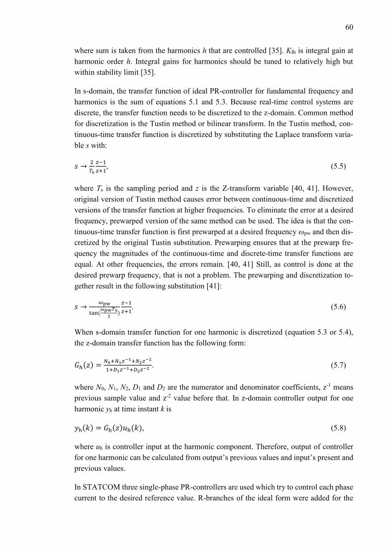
60

where sum is taken from the harmonics h that are controlled [35]. KIh is integral gain at

harmonic order h. Integral gains for harmonics should be tuned to relatively high but

within stability limit [35].

In s-domain, the transfer function of ideal PR-controller for fundamental frequency and

harmonics is the sum of equations 5.1 and 5.3. Because real-time control systems are

discrete, the transfer function needs to be discretized to the z-domain. Common method

for discretization is the Tustin method or bilinear transform. In the Tustin method, con-

tinuous-time transfer function is discretized by substituting the Laplace transform varia-

ble s with:

𝑠 →2

𝑇s

𝑧−1

𝑧+1, (5.5)

where Ts is the sampling period and z is the Z-transform variable [40, 41]. However,

original version of Tustin method causes error between continuous-time and discretized

versions of the transfer function at higher frequencies. To eliminate the error at a desired

frequency, prewarped version of the same method can be used. The idea is that the con-

tinuous-time transfer function is first prewarped at a desired frequency ωpw and then dis-

cretized by the original Tustin substitution. Prewarping ensures that at the prewarp fre-

quency the magnitudes of the continuous-time and discrete-time transfer functions are

equal. At other frequencies, the errors remain. [40, 41] Still, as control is done at the

desired prewarp frequency, that is not a problem. The prewarping and discretization to-

gether result in the following substitution [41]:

𝑠 →𝜔pw

tan(𝜔pw𝑇s

2)

𝑧−1

𝑧+1. (5.6)

When s-domain transfer function for one harmonic is discretized (equation 5.3 or 5.4),

the z-domain transfer function has the following form:

𝐺ℎ(𝑧) =𝑁0+𝑁1𝑧−1+𝑁2𝑧−2

1+𝐷1𝑧−1+𝐷2𝑧−2 . (5.7)

where N0, N1, N2, D1 and D2 are the numerator and denominator coefficients, z-1 means

previous sample value and z-2 value before that. In z-domain controller output for one

harmonic yh at time instant k is

𝑦h(𝑘) = 𝐺h(𝑧)𝑢h(𝑘), (5.8)

where uh is controller input at the harmonic component. Therefore, output of controller

for one harmonic can be calculated from output’s previous values and input’s present and

previous values.

In STATCOM three single-phase PR-controllers are used which try to control each phase

current to the desired reference value. R-branches of the ideal form were added for the

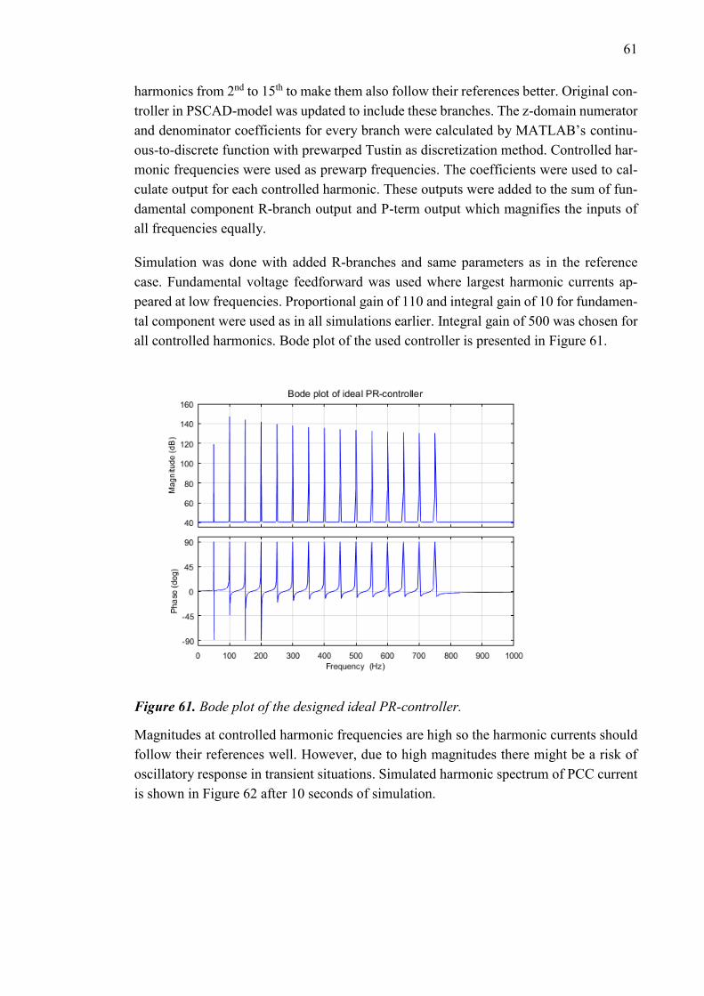
61

harmonics from 2nd to 15th to make them also follow their references better. Original con-

troller in PSCAD-model was updated to include these branches. The z-domain numerator

and denominator coefficients for every branch were calculated by MATLAB’s continu-

ous-to-discrete function with prewarped Tustin as discretization method. Controlled har-

monic frequencies were used as prewarp frequencies. The coefficients were used to cal-

culate output for each controlled harmonic. These outputs were added to the sum of fun-

damental component R-branch output and P-term output which magnifies the inputs of

all frequencies equally.

Simulation was done with added R-branches and same parameters as in the reference

case. Fundamental voltage feedforward was used where largest harmonic currents ap-

peared at low frequencies. Proportional gain of 110 and integral gain of 10 for fundamen-

tal component were used as in all simulations earlier. Integral gain of 500 was chosen for

all controlled harmonics. Bode plot of the used controller is presented in Figure 61.

Figure 61. Bode plot of the designed ideal PR-controller.

Magnitudes at controlled harmonic frequencies are high so the harmonic currents should

follow their references well. However, due to high magnitudes there might be a risk of

oscillatory response in transient situations. Simulated harmonic spectrum of PCC current

is shown in Figure 62 after 10 seconds of simulation.

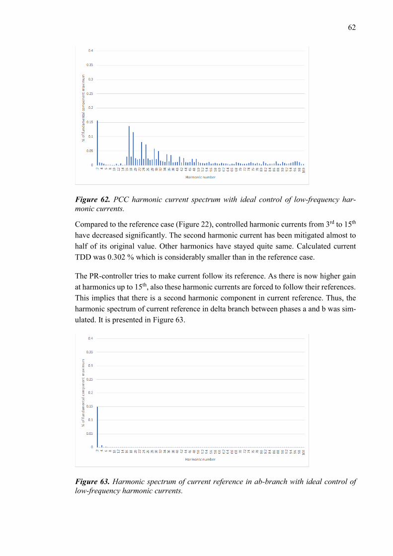
62

Figure 62. PCC harmonic current spectrum with ideal control of low-frequency har-

monic currents.

Compared to the reference case (Figure 22), controlled harmonic currents from 3rd to 15th

have decreased significantly. The second harmonic current has been mitigated almost to

half of its original value. Other harmonics have stayed quite same. Calculated current

TDD was 0.302 % which is considerably smaller than in the reference case.

The PR-controller tries to make current follow its reference. As there is now higher gain

at harmonics up to 15th, also these harmonic currents are forced to follow their references.

This implies that there is a second harmonic component in current reference. Thus, the

harmonic spectrum of current reference in delta branch between phases a and b was sim-

ulated. It is presented in Figure 63.

Figure 63. Harmonic spectrum of current reference in ab-branch with ideal control of

low-frequency harmonic currents.

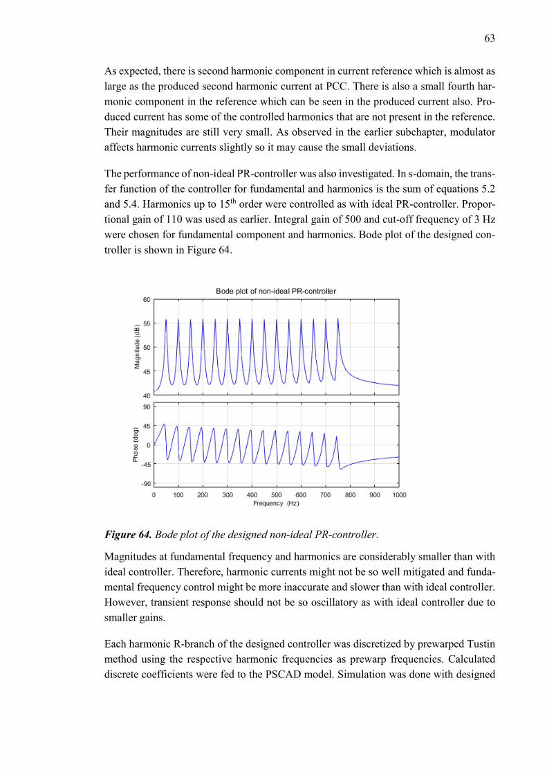
63

As expected, there is second harmonic component in current reference which is almost as

large as the produced second harmonic current at PCC. There is also a small fourth har-

monic component in the reference which can be seen in the produced current also. Pro-

duced current has some of the controlled harmonics that are not present in the reference.

Their magnitudes are still very small. As observed in the earlier subchapter, modulator

affects harmonic currents slightly so it may cause the small deviations.

The performance of non-ideal PR-controller was also investigated. In s-domain, the trans-

fer function of the controller for fundamental and harmonics is the sum of equations 5.2

and 5.4. Harmonics up to 15th order were controlled as with ideal PR-controller. Propor-

tional gain of 110 was used as earlier. Integral gain of 500 and cut-off frequency of 3 Hz

were chosen for fundamental component and harmonics. Bode plot of the designed con-

troller is shown in Figure 64.

Figure 64. Bode plot of the designed non-ideal PR-controller.

Magnitudes at fundamental frequency and harmonics are considerably smaller than with

ideal controller. Therefore, harmonic currents might not be so well mitigated and funda-

mental frequency control might be more inaccurate and slower than with ideal controller.

However, transient response should not be so oscillatory as with ideal controller due to

smaller gains.

Each harmonic R-branch of the designed controller was discretized by prewarped Tustin

method using the respective harmonic frequencies as prewarp frequencies. Calculated

discrete coefficients were fed to the PSCAD model. Simulation was done with designed

64

controller and same parameters as in the reference case. Simulated PCC current is pre-

sented in Figure 65.

Figure 65. PCC harmonic current spectrum with non-ideal control of low-frequency har-

monic currents.

Controlled harmonic currents have decreased significantly compared to the reference

case. Still, mitigation is not as good as with ideal PR-controller. Produced second har-

monic current is almost as large as with ideal control and it results from the second har-

monic in current reference as observed earlier. Other harmonic currents which were not

controlled have increased a bit. Current TDD was 0.432 % which is 43 % higher than

with ideal control. Used integral gain for harmonics was chosen to be same as with ideal

control for comparison. It was not optimized with respect to harmonic performance so it

may still be possible to increase gains at harmonics to decrease currents.

Theoretically, all harmonic currents could be removed by adding R-branches to current

controller for all harmonics. Exceptions are the second and fourth harmonic which are

present in the reference and the small harmonic currents caused by modulator. However,

in reality the measurement for harmonics may not be so accurate as for fundamental com-

ponent which may deteriorate the performance of current control. Harmonic currents are

tried to be controlled to zero or at least almost to zero so the sensor should be very sensi-

tive at harmonics. At the same time, the sensor should accurately measure small DC-

component and the fundamental component which can be up to 1000 A RMS. Currently

used LEM ITL-4000-S fluxgate current transducer’s sensitivity is almost 0 dB up to 10

kHz as can be seen from Figure 66 [42]. However, the sensitivity is measured with 40 A

RMS primary current so characteristics might be worse for smaller currents.

65

Figure 66. LEM ITL-4000-S current transducer’s sensitivity in decibels as function of

frequency [42].

5.3 DC-link voltage control effect

In the earlier subchapter it was found out that there are second and fourth harmonic com-

ponents in current reference. As manual current q-component control is used and q-com-

ponent reference is kept constant, the harmonics must come either from the synchroniza-

tion to secondary busbar voltage or the controllers which control total DC-voltages of

MMC branches to nominal values.

Effect of DC-link voltage control can be removed by setting all submodule voltages con-

stant. Then, total DC-voltages of each branch stay constant all the time and controlling of

branch voltages is not needed. This affects modulator a bit also because DC-voltages of

submodules do not change and thus they are not needed to be balanced either.

Submodule voltages were forced to stay at their nominal values and current control with

ideal PR-controller for harmonics from 2nd to 15th was used with same parameters as be-

fore. Simulated PCC current harmonic spectrum is presented in Figure 67.

66

Figure 67. Harmonic spectrum of PCC current with constant DC-voltages and low-fre-

quency harmonic current control.

Second harmonic current has decreased to same order of magnitude as other low-order

harmonics. This result confirms that controlling of branch DC-voltages causes the second

harmonic to increase. Harmonic spectrum of current reference in ab-branch in this case

is shown in Figure 68.

Figure 68. Harmonic spectrum of current reference with constant DC-voltages and low-

frequency harmonic current control.

Second and fourth harmonic components have disappeared from the reference. Rest of

the harmonics from 2nd to 15th order appearing in PCC current are thus result of modulator

operation or errors in current control.

67

DC-link voltage control consists of two controllers so the exact origin of second harmonic

current was investigated. In the current reference, second harmonic could be any se-

quence. However, second harmonic appears in PCC current also. Therefore, it can not be

zero sequence since zero sequence current can not escape the delta connected STATCOM

or flow through the star-delta connected transformer. Thus, second harmonic should be a

result of control which balances the average of DC-voltages in three branches and pro-

duces current d-component reference. Consequently, simulation with ideal PR-control for

harmonics up to 15th order was repeated and the spectrum of current d-component refer-

ence transformed to the stationary frame was recorded. The reference current term in sta-

tionary frame id,ab,ref due to current d-component reference id,ref is calculated as follows:

𝑖d,ab,ref = √2𝑖d,ref sin(𝜔1𝑡 + 𝜃), (5.9)

where ω1 is the fundamental angular frequency, t time and θ angle provided by synchro-

nization to secondary busbar. The spectrum of the reference is shown in Figure 69.

Figure 69. Harmonic spectrum of current d-component reference in stationary frame

with low-frequency harmonic current control.

Second and fourth harmonics are almost same magnitude as in the total current reference.

These harmonics are therefore a result of controlling the average of DC-voltages in three

MMC branches to the nominal value. As the harmonics participate in DC-link voltage

control in STATCOM, it may be difficult to remove them.

However, it was observed in chapter 4.1 that when grid voltage is sinusoidal, second har-

monic current is very small. So, it seems that DC-link voltage control does not increase

second harmonic current when there are not harmonic voltages present in grid. It was

further studied by repeating the simulation in capacitive operating point with sinusoidal

grid voltage. Simulated current reference in ab-branch is shown in Figure 70.

68

Figure 70. Harmonic spectrum of current reference with sinusoidal grid voltage.

Second harmonic current is negligible in the reference. It can be concluded that second

harmonic current increases due to combined effect of harmonic voltages in grid and con-

trol of average DC-voltage in three MMC branches.

5.4 Voltage control effect

Investigation of voltage control effect on harmonic current emissions is quite simple. In

all previous simulations manual current q-component control was used. It is only needed

to switch on the voltage control function which provides the current q-component refer-

ence. First, simulation was done with voltage reference of 1.05 p.u which resulted in 993

A capacitive current in STATCOM’s delta branch. The operating point is thus almost

same as in the reference case. Harmonic current spectrum at PCC is shown in Figure 71.

69

Figure 71. Harmonic spectrum of PCC current with voltage control (1.05 p.u voltage

reference).

Calculated current TDD was 0.800 % which is almost same as in the reference case.

Moreover, the spectrum resembles reference case spectrum. Low-order harmonics have

increased or decreased slightly compared to it.

However, voltage controller provides current q-component reference and can add har-

monics to it. These harmonics are not seen well in the output current because current

controller’s gain is low at harmonics. Therefore, also the harmonic spectrum of current

reference in ab-branch was recorded. It is presented in Figure 72.

Figure 72. Harmonic spectrum of current reference with voltage control (1.05 p.u voltage

reference).

Low-order harmonics, especially the third harmonic, have increased in the reference com-

pared to manual current q-component control. However, second harmonic has increased

70

only little since there was already a second harmonic component in the reference with

manual current q-component control. As the other low-order harmonics increased but

second harmonic did not, harmonic spectrums of the d-, q- and zero-component refer-

ences were investigated to understand the phenomenon. Current d-component in station-

ary frame was calculated according to equation 5.9 and q-component reference in station-

ary frame iq,ab,ref was calculated as follows:

𝑖q,ab,ref = √2𝑖q,ref cos(𝜔1𝑡 + 𝜃), (5.10)

where iq,ref is current q-component reference in synchronous frame. Spectrums of the ref-

erence components up to 10th harmonic are presented in Figure 73.

Figure 73. Harmonic spectrums of current d-, q-, and zero-component references with

voltage control (1.05 p.u voltage reference).

Second harmonic is substantially larger in q-component reference than in the total current

reference. It seems that the second harmonic reference components cancel each other

partly so that the total second harmonic reference is smaller than the q-component refer-

ence.

Next, effect of voltage control was studied in another operating point. Simulation was

done with voltage reference of 1.0 p.u which resulted in 20 A inductive-resistive current

in STATCOM’s delta branch. Harmonic current spectrum at PCC is shown in Figure 74.

a) d-component reference b) q-component reference c) zero-component reference

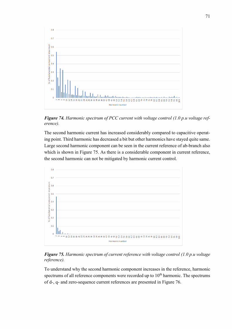
71

Figure 74. Harmonic spectrum of PCC current with voltage control (1.0 p.u voltage ref-

erence).

The second harmonic current has increased considerably compared to capacitive operat-

ing point. Third harmonic has decreased a bit but other harmonics have stayed quite same.

Large second harmonic component can be seen in the current reference of ab-branch also

which is shown in Figure 75. As there is a considerable component in current reference,

the second harmonic can not be mitigated by harmonic current control.

Figure 75. Harmonic spectrum of current reference with voltage control (1.0 p.u voltage

reference).

To understand why the second harmonic component increases in the reference, harmonic

spectrums of all reference components were recorded up to 10th harmonic. The spectrums

of d-, q- and zero-sequence current references are presented in Figure 76.

72

Figure 76. Harmonic spectrums of current d-, q-, and zero-component references with

voltage control (1.0 p.u voltage reference).

Second harmonic in current q-component reference has increased a bit compared to ca-

pacitive operating point. Second harmonic has decreased significantly in current d-com-

ponent and a bit in zero-component reference. It seems that the total second harmonic

current reference increases because other reference components cancel smaller part of the

q-component reference second harmonic than in the capacitive operating point.

Simulation was done also with 0.95 p.u voltage reference. It resulted in 954 A inductive

current in delta branch. Harmonic current spectrum at PCC is presented in Figure 77 and

reference current spectrum in Figure 78.

Figure 77. Harmonic spectrum of PCC current with voltage control (0.95 p.u voltage

reference).

a) d-component reference b) q-component reference c) zero-component reference

73

Figure 78. Harmonic spectrum of current reference with voltage control (0.95 p.u voltage

reference).

Second harmonic current and its reference are even larger in this operating point. Again,

all reference component harmonic spectrums were recorded up to 10th harmonic to see

the composition of total second harmonic reference. They are shown in Figure 79.

Figure 79. Harmonic spectrums of current d-, q-, and zero-component references with

voltage control (0.95 p.u voltage reference).

Second harmonic in d-component reference has increased to same level as in capacitive

operating point. Second harmonic in q- and zero- components have stayed quite same as

in the previous operating point. It seems that in this inductive operating point second

harmonic reference components do not cancel each other like in capacitive operating

a) d-component reference b) q-component reference c) zero-component reference

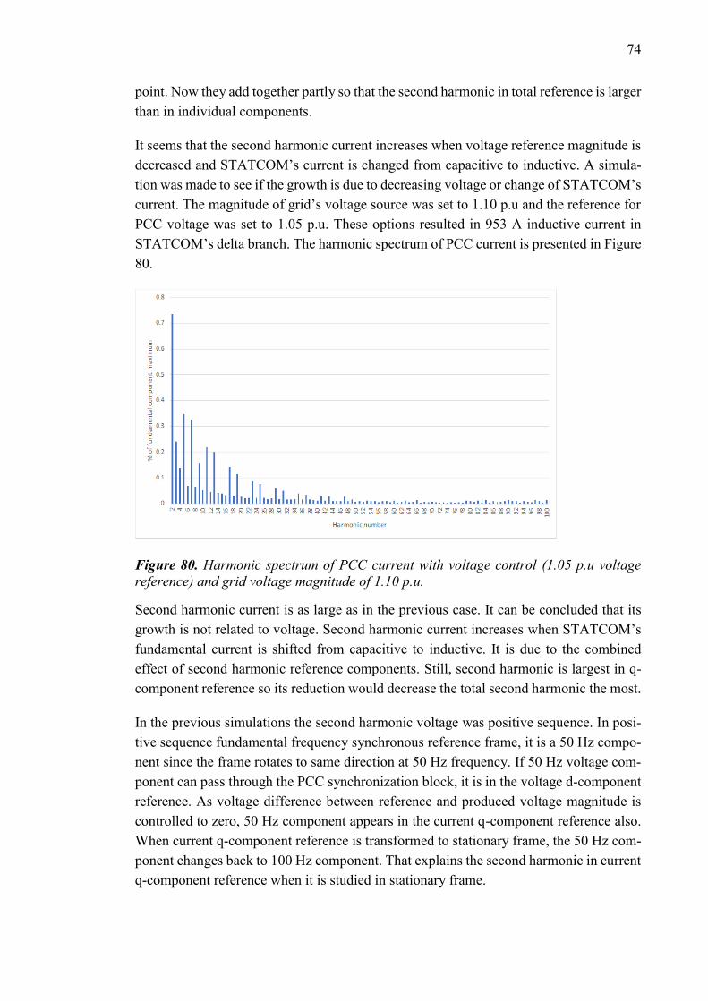
74

point. Now they add together partly so that the second harmonic in total reference is larger

than in individual components.

It seems that the second harmonic current increases when voltage reference magnitude is

decreased and STATCOM’s current is changed from capacitive to inductive. A simula-

tion was made to see if the growth is due to decreasing voltage or change of STATCOM’s

current. The magnitude of grid’s voltage source was set to 1.10 p.u and the reference for

PCC voltage was set to 1.05 p.u. These options resulted in 953 A inductive current in

STATCOM’s delta branch. The harmonic spectrum of PCC current is presented in Figure

80.

Figure 80. Harmonic spectrum of PCC current with voltage control (1.05 p.u voltage

reference) and grid voltage magnitude of 1.10 p.u.

Second harmonic current is as large as in the previous case. It can be concluded that its

growth is not related to voltage. Second harmonic current increases when STATCOM’s

fundamental current is shifted from capacitive to inductive. It is due to the combined

effect of second harmonic reference components. Still, second harmonic is largest in q-

component reference so its reduction would decrease the total second harmonic the most.

In the previous simulations the second harmonic voltage was positive sequence. In posi-

tive sequence fundamental frequency synchronous reference frame, it is a 50 Hz compo-

nent since the frame rotates to same direction at 50 Hz frequency. If 50 Hz voltage com-

ponent can pass through the PCC synchronization block, it is in the voltage d-component

reference. As voltage difference between reference and produced voltage magnitude is

controlled to zero, 50 Hz component appears in the current q-component reference also.

When current q-component reference is transformed to stationary frame, the 50 Hz com-

ponent changes back to 100 Hz component. That explains the second harmonic in current

q-component reference when it is studied in stationary frame.

75

Synchronization includes a first-order low-pass filter for produced voltage d-component.

Used time constant of the filter was 0.01 seconds in the simulations. Transfer function of

the used filter is therefore

𝐿𝑃𝐹(𝑠) =1

1+0.01𝑠. (5.11)

Its magnitude is

|𝐿𝑃𝐹(𝜔)| =1

√1+0.0001𝜔2. (5.12)

Magnitude at 50 Hz, which corresponds to positive sequence second harmonic in the syn-

chronous frame, is

|𝐿𝑃𝐹(50𝐻𝑧)| =1

√1+0.0001∗(2𝜋∗50)2= 0.303. (5.13)

Therefore, part of the 50 Hz component can pass through the low-pass filter. The 50 Hz

component in voltage d-component and the second harmonic in current q-component ref-

erence can be decreased by increasing the low-pass filter’s time constant and thus de-

creasing its gain at 50 Hz. However, increasing the time constant slows down the transient

response of the synchronization [43].

If second harmonic voltage is negative sequence, it rotates to another direction as positive

sequence fundamental synchronous reference frame. In the frame, it is thus a 150 Hz

component. As the frequency is higher, the low-pass filter for voltage d-component

should mitigate the component better. Figure 81 presents the harmonic spectrum of sim-

ulated PCC current when all grid harmonic voltages were same magnitude as before but

negative sequence. Grid voltage was 1.0 p.u and reference for PCC voltage was 0.95 p.u

as in the worst case simulated for positive sequence harmonics.

76

Figure 81. Harmonic spectrum of PCC current with voltage control (0.95 p.u voltage

reference) and negative sequence harmonic voltages.

Second harmonic current is substantially smaller than with positive sequence harmonic

voltages. Magnitudes of other harmonic currents are quite same as with positive sequence

harmonics. Current reference in ab-branch is shown in Figure 82.

Figure 82. Harmonic spectrum of current reference with voltage control (0.95 p.u voltage

reference) and negative sequence harmonic voltages.

The second harmonic has decreased considerably in the reference also. The third har-

monic has increased over 50 % compared to positive sequence case but its magnitude is

still quite low.

In perfectly balanced three-phase system second harmonic voltage is negative sequence

[4]. According to previous simulation, it would not be a problem then. However, in un-

balanced system, the second harmonic voltage may appear at any sequence. As observed,

77

large positive sequence second harmonic voltage causes large current at same frequency

in inductive operating point. That may cause noncompliance with standards or specifica-

tions.

A solution was developed to decrease the second harmonic in current q-component ref-

erence and thus in produced current. A band-stop filter was designed for the voltage d-

component that synchronization produces. Design was done with MATLAB’s Filter De-

signer tool. Positive sequence second harmonic voltage appears in fundamental frequency

synchronous frame as 50 Hz component so filter’s lowest magnitude was designed to 50

Hz. Butterworth 2nd order filter was chosen with lower cut-off frequency of 40 Hz and

higher cut-off frequency of 62 Hz. The magnitude response of the filter is shown in Figure

83.

Figure 83. Magnitude response of the designed band-stop filter.

The most important restriction for the filter is that it should not affect voltage DC-com-

ponent at all because that would deteriorate the accuracy of fundamental voltage control.

As can be seen from the magnitude response, the magnitude of the designed filter is very

close to zero decibel at 0 Hz. In addition, filter offers over 30 dB attenuation at 50 Hz.

A simulation was done with the designed filter in the worst-case operation point with

respect to second harmonic current generation. Voltage reference was set to 0.95 p.u, grid

voltage magnitude to 1.0 p.u and positive sequence harmonic voltages were added in grid.

The simulated harmonic spectrum of PCC current is presented in Figure 84 and spectrum

of reference current in ab-branch in Figure 85.

78

Figure 84. Harmonic spectrum of PCC current with voltage control (0.95 p.u voltage

reference) and band-stop filter.

Figure 85. Harmonic spectrum of current reference with voltage control (0.95 p.u voltage

reference) and band-stop filter.

Second harmonic has decreased considerably both in PCC and reference currents. Pro-

duced second harmonic current is almost as small as in capacitive operating point without

filter. The remaining second harmonic current in the reference was identified earlier to be

result of DC-link voltage control. Now, second harmonic current could be also further

attenuated by current control as its reference is smaller than produced current.

Since filter was added to voltage control path, delay was introduced. Therefore, filter’s

effect on dynamic performance of voltage control was investigated. A step test was done

where voltage reference was changed from 0.95 p.u to 1.05 p.u after 0.5 seconds of sim-

ulation. Measured voltage d-component magnitude at PCC during step test without and

with filter are presented in Figure 86.

79

Figure 86. Dynamic behavior of measured voltage d-component magnitude during step

test without (upper figure) and with (lower figure) band-stop filter.

Control delay is so small that it can not be seen from the figure. In the figure, measured

voltage d-component is smoother with filter because second harmonic is filtered from the

voltage. Alternative option for 50 Hz component filtering would have been a low-pass

filter with lower cut-off frequency than currently used. To achieve same attenuation at 50

Hz with it, very small cut-off frequency and higher filter order should have been used.

That would have decreased the filter’s gain at lower frequencies also and slowed down

the voltage response more.

80

6. FUTURE WORK

There are still some ideas to improve harmonic performance which were not possible to

test in the given time frame or were decided not to be included in the thesis. These ideas

are introduced in this chapter.

Harmonic voltages at PCC can be reduced by actively filtering them. The idea of active

filtering is to inject harmonic currents from the converter so that they cause harmonic

voltage drops in grid impedances which cancel the harmonic voltages at PCC [39]. It is

important to know the grid impedance angles at controlled harmonics as they determine

the phase differences between produced currents and voltage drops [39].

Secondary busbar synchronization effect on harmonic currents was not studied in the the-

sis because the synchronization implementation had been simplified in the used PSCAD

model. Its effect could be studied by building the real synchronization block to the model

and comparing the results with the quite ideal one used in this model.

Modulator’s effect on harmonic currents was observed to be small if there are harmonics

of same order in grid voltage. However, if there is not a voltage component at some har-

monic present, modulator causes still some current at that frequency. The problem of the

modulator is that it produces small currents at all harmonics. If there are some frequencies

where current should not be produced, the modulator prevents that possibility. As ex-

plained before there are some alternative modulator schemes where harmonic currents

caused by the modulator could be shifted to higher frequencies and thus zero current

emissions at some harmonics could be achieved.

Non-ideal current controller, introduced in chapter 5.2, can control harmonic currents

even though frequencies of harmonic components change a bit. Harmonic performance

of the STATCOM system with non-ideal controller could be tested when harmonic fre-

quencies are varied slightly.

81

7. CONCLUSIONS

The studied problem in this thesis was that harmonic currents of STATCOM increase

considerably when harmonics are added to grid voltage. These harmonic currents cause

harmonic voltages at impedances of grid components. The limits for harmonic currents

in reactive power compensation applications originate usually from the limits for PCC

harmonic voltages which are stated in standards and transmission operators’ specifica-

tions. The harmonic voltages caused by STATCOM are usually added to existing har-

monic voltages at PCC. If the existing harmonic voltages are large, the limits for STAT-

COM produced harmonic voltages and currents are strict. The problem, its reasons and

solutions were investigated by simulations in PSCAD.

One major topic studied was the comparison of secondary busbar voltage feedforward

options. The considered options are instantaneous value of the voltage or the fundamental

component of it. The fundamental component feedforward seemed to have some desirable

characteristics such as predictability of the produced harmonic current spectrum, better

current mitigation at harmonic orders from 20 to 40 and no need for harmonic voltage

measurement. Its disadvantage is that low-order harmonic currents are large if there are

large low-order harmonic voltages in grid. With fundamental feedforward, produced har-

monic currents decreased harmonic voltages at PCC at most frequencies but only if grid

is inductive-resistive. Grid’s harmonic impedances change over time and have also ca-

pacitive values. In that case, produced currents cause increasing harmonic voltages at

PCC. Although grid impedances might be mostly inductive, harmonic limits must be re-

spected in every grid contingency.

The idea of instantaneous voltage feedforward is that harmonic voltages over coupling

reactor would be zero and harmonic currents would not be induced. As observed, used

modulator execution frequency causes too much delay so that the feedforward would

work as planned for higher order harmonics. Still, harmonic currents up to 20th order were

smaller than with fundamental feedforward. Harmonic currents decreased considerably

when modulator execution frequency was doubled and instantaneous feedforward was

used. However, switching frequency was doubled and thus losses were increased substan-

tially. Moreover, real life harmonic voltage measurement can be inaccurate and other

possible delays can deteriorate the performance more.

The advantages of feedforward options were tried to be combined by using a low-pass

filter for the voltage feedforward. A low-pass filter was designed to reject high frequency

noise and reduce the effect of feedforward at high-order harmonics. As a result, low-order

harmonics were mitigated compared to fundamental feedforward and harmonics around

30th decreased compared to instantaneous feedforward. Still, low-order harmonics up to

20th order increased in comparison with instantaneous feedforward due to filter delay.

82

One simple solution to decrease harmonic currents is to increase the coupling reactor’s

inductance. Current controller’s proportional gain must be increased with same amount

in percent to have considerable effect on harmonics and same dynamic performance as

with original reactor. Disadvantage of the higher inductance is that more reactor material

and more submodules in converter are needed so costs are increased.

The effect of modulator on harmonics was studied by idealizing it. Ideal modulator pro-

duces exactly the reference voltage every simulation step and keeps submodule voltages

constant. It was observed that with fundamental voltage feedforward all harmonic cur-

rents could be removed if grid voltage was sinusoidal. However, when there were har-

monic voltages in grid, modulator had only a minor effect on harmonic currents. With

instantaneous feedforward and ideal modulator all harmonic currents could be removed

even if harmonic voltages appeared in grid. So, modulator’s effect on harmonics is mainly

its delay which deteriorates the feedforward of harmonic voltages. Moreover, it causes

small currents at all harmonics even though grid voltage is sinusoidal.

Current control with added resonant branches for harmonics seemed to work very well

for low-order harmonics when current measurement was ideal. Better mitigation was

achieved with ideal resonant branches but non-ideal branches should be more stable and

work even if frequencies vary a bit. Fundamental voltage feedforward can be used so

harmonic voltage measurement is not needed. Measuring the quite small harmonic com-

ponents accurately from large total current might still be a challenge in a real system.

Harmonic current control could not remove the second harmonic component. This com-

ponent was present in current reference and thus the second harmonic was controlled to

the reference value. Origin of this component in the reference was identified to be the

control function which controls the average of DC-voltages in three STATCOM delta

branches to the nominal value. However, second harmonic current was not present in the

reference when grid voltage was sinusoidal. Therefore, the second harmonic is due to the

combination of harmonic voltages in grid and DC-link voltage control.

Voltage control had no significant effect on produced harmonic currents except for sec-

ond harmonic. It was observed that second harmonic current increases when the operating

point is shifted from capacitive to inductive. Voltage controller caused quite large second

harmonic to current q-component reference when there was a positive sequence second

harmonic voltage in grid. In capacitive point, d- and zero-components canceled the sec-

ond harmonic in q-component partly so that the total reference was smaller than the q-

component. In inductive point, reference components were partly summed together so the

total second harmonic current reference increased. When second harmonic voltage in grid

was negative sequence, produced second harmonic current was significantly smaller. The

problem was solved by adding a band-stop filter for voltage d-component at 50 Hz which

efficiently mitigated the second harmonic current.

83

REFERENCES

[1] B. Singh, A. Chandra, K. Al-Haddad, Power Quality : Problems and Mitigation

Techniques, John Wiley & Sons, New York, 2014, 599 p.

[2] CIGRE Working Group 14.19, Static Synchronous Compensator (STATCOM),

CIGRE, 2000, 211 p.

[3] E. Fuchs, M.A.S. Masoum, Power Quality in Power Systems and Electrical Ma-

chines, Elsevier Science, San Diego, 2008, 659 p.

[4] S. Santoso, M.F. McGranaghan, R.C. Dugan, H.W. Beaty, Electrical Power Systems

Quality, Third Edition, McGraw-Hill Education, 2012, 528 p.

[5] T. Dao, B.T. Phung, T. Blackburn, Effects of voltage harmonics on distribution

transformer losses, Proceedings of the Power and Energy Engineering Conference (AP-

PEEC), 2015 IEEE PES Asia-Pacific, Brisbane, Australia, November 15–18, 2015,

IEEE, pp. 1-5.

[6] M.A. Prša, K.K. Kasaš-Lažetić, N.D. Mučalica, Skin effect and proximity effect in a

real, high voltage, double three-phase system, Proceedings of the EUROCON - Interna-

tional Conference on Computer as a Tool (EUROCON), Lisbon, Portugal, April 27–29,

2011, IEEE, pp. 1-4.

[7] K.D. Patil, W.Z. Gandhare, Threat of harmonics to underground cables, Proceedings

of the 2012 Students Conference on Engineering and Systems, Allahabad, India, March

16-18, 2012, IEEE, pp. 1-6.

[8] Sumaryadi, H. Gumilang, A. Suslilo, Effect of power system harmonic on degrada-

tion process of transformer insulation system, Proceedings of the 9th International Con-

ference on the Properties and Applications of Dielectric Materials, Harbin, China, July

19–23, 2009, IEEE, pp. 261-264.

[9] S. Chattopadhyay, M. Mitra, S. Sengupta, Electric Power Quality, Springer Nether-

lands, 2011, 179 p.

[10] De La Rosa, Harmonics and Power Systems, CRC Press, 2006, 179 p.

[11] F. Lin, S. Zuo, W. Deng, S. Wu, Modeling and Analysis of Electromagnetic Force,

Vibration, and Noise in Permanent-Magnet Synchronous Motor Considering Current

Harmonics, IEEE Transactions on Industrial Electronics, Vol. 63, Iss. 12, 2016, pp.

7455-7466.

[12] M. Ertl, S. Voss, The role of load harmonics in audible noise of electrical trans-

formers, Journal of Sound and Vibration, Vol. 333, Iss. 8, 2014, pp. 2253-2270.

84

[13] A. Fidigatti, E. Ragaini, Effect of harmonic pollution on low voltage overcurrent

protection, Proceedings of the 14th International Conference on Harmonics and Quality

of Power - ICHQP, Bergamo, Italy, September 26–29, 2010, IEEE, pp. 1-4.

[14] IEEE 519, Recommended Practice and Requirements for Harmonic Control in

Electric Power Systems, IEEE, 2014, 29 p.

[15] IEC 61000-2-2, Compatibility levels for low-frequency conducted disturbances and

signalling in public low-voltage power supply systems, IEC, 2017, 36 p.

[16] IEC 61000-2-4, Compatibility levels in industrial plants for low-frequency con-

ducted disturbances, IEC, 2002, 75 p.

[17] IEC 61000-2-12, Environment – Compatibility levels for low-frequency conducted

disturbances and signalling in public medium-voltage power supply systems, IEC, 2003,

55 p.

[18] IEC 61000-3-2, Limits – Limits for harmonic current emissions (equipment input

current ≤ 16 A per phase), IEC, 2014, 34 p.

[19] IEC 61000-3-12, Limits – Limits for harmonic currents produced by equipment

connected to public low-voltage systems with input current >16 A and ≤75 A per phase,

IEC, 2011, 25 p.

[20] IEC/TR 61000-3-6, Limits – Assessment of emission limits for the connection of

distorting installations to MV, HV and EHV power systems, IEC, 2008, 58 p.

[21] W. Hofmann, W. Just, Reactive Power Compensation : A Practical Guide, Wiley,

Hoboken, 2012, 288 p.

[22] S. Corsi, Voltage Control and Protection in Electrical Power Systems, Springer

Verlag, 2015, 557 p.

[23] J. Dixon, L. Moran, J. Rodriguez, R. Domke, Reactive Power Compensation Tech-

nologies: State-of-the-Art Review, Proceedings of the IEEE, Vol. 93, Iss. 12, 2005, pp.

2144-2164.

[24] R. Smeets, L. van der Sluis, M. Kapetanovic, Switching in Electrical Transmission

and Distribution Systems, John Wiley & Sons, New York, 2014, 425 p.

[25] CIGRE Working Group 14.30, Guide to the Specification and Design Evaluation

of AC Filters for HVDC Systems, CIGRE, 1999, 251 p.

[26] R.S. Thallam, G. Joós, Reactive Power Compensation, in: L. Grigsby (ed.), Electric

Power Generation, Transmission, and Distribution, CRC Press, 2012, pp. 789.

[27] D.P. Kothari, I.J. Nagrath, Modern Power System Analysis, Third ed. Tata

McGraw-Hill Publishing Company Limited, New Delhi, 2003, 694 p.

85

[28] R.M. Mathur, R.K. Varma, Thyristor-Based FACTS Controllers for Electrical

Transmission Systems, IEEE, Piscataway, NJ, 2002, 505 p.

[29] CIGRE Working Group 38-01 Task Force No. 2, Static Var Compensators, CI-

GRE, 1986, 128 p.

[30] E. Barrios-Martínez, C. Ángeles-Camacho, Technical comparison of FACTS con-

trollers in parallel connection, Journal of Applied Research and Technology, Vol. 15,

Iss. 1, 2017, pp. 36-44.

[31] B. Singh, R. Saha, A. Chandra, K. Al-Haddad, Static synchronous compensators

(STATCOM): a review, IET Power Electronics, Vol. 2, Iss. 4, 2009, pp. 297-324.

[32] S. Khomfoi, L.M. Tolbert, Multilevel Power Converters, in: M.H. Rashid (ed.),

Power Electronics Handbook, Elsevier Science, 2011, pp. 455-486.

[33] M. Hagiwara, H. Akagi, Control and Experiment of Pulsewidth-Modulated Modu-

lar Multilevel Converters, IEEE Transactions on Power Electronics, Vol. 24, Iss. 7,

2009, pp. 1737-1746.

[34] K. Sharifabadi, L. Harnefors, H. Nee, S. Norrga, R. Teodorescu, Design, Control,

and Application of Modular Multilevel Converters for HVDC Transmission Systems,

IEEE Press, United Kingdom, 2016, 386 p.

[35] R. Teodorescu, F. Blaabjerg, M. Liserre, P.C. Loh, Proportional-resonant control-

lers and filters for grid-connected voltage-source converters, IEE Proceedings - Electric

Power Applications, Vol. 153, Iss. 5, 2006, pp. 750-762.

[36] E. Twining, D.G. Holmes, Grid current regulation of a three-phase voltage source

inverter with an LCL input filter, IEEE Transactions on Power Electronics, Vol. 18, Iss.

3, 2003, pp. 888-895.

[37] X. Wang, X. Ruan, S. Liu, C.K. Tse, Full Feedforward of Grid Voltage for Grid-

Connected Inverter With LCL Filter to Suppress Current Distortion Due to Grid Volt-

age Harmonics, IEEE Transactions on Power Electronics, Vol. 25, Iss. 12, 2010, pp.

3119-3127.

[38] Q. Yan, X. Wu, X. Yuan, Y. Geng, An Improved Grid-Voltage Feedforward Strat-

egy for High-Power Three-Phase Grid-Connected Inverters Based on the Simplified Re-

petitive Predictor, IEEE Transactions on Power Electronics, Vol. 31, Iss. 5, 2016, pp.

3880-3897.

[39] A. Tarkiainen, R. Pollanen, M. Niemela, J. Pyrhonen, Identification of grid imped-

ance for purposes of voltage feedback active filtering, IEEE Power Electronics Letters,

Vol. 2, Iss. 1, 2004, pp. 6-10.

[40] C. Korlinchak, M. Comanescu, Discrete time integration of observers with continu-

ous feedback based on Tustin's method with variable prewarping, Proceedings of the 6th

IET International Conference on Power Electronics, Machines and Drives, Bristol,

86

United Kingdom, March 27-29, 2012, The Institution of Engineering & Technology, pp.

1-6.

[41] W.Y. Yang, Continuous-Time Systems and Discrete-Time Systems, in: W.Y. Yang

(ed.), Signals and Systems with MATLAB, Springer, Berlin, 2009, pp. 277-306.

[42] Current Transducer ITL 4000-S Datasheet, LEM, 2017, 8 p. Available:

http://www.lem.com/docs/products/itl_4000-s.pdf.

[43] P. Rodriguez, J. Pou, J. Bergas, J.I. Candela, R.P. Burgos, D. Boroyevich, Decou-

pled Double Synchronous Reference Frame PLL for Power Converters Control, IEEE

Transactions on Power Electronics, Vol. 22, Iss. 2, 2007, pp. 584-592.

87

APPENDIX A: CONTROL BLOCK DIAGRAM

Appendix A, Figure 1. Control block diagram of STATCOM.

Syn

chro

ni-

zati

on

to

P

CC

vo

ltag

e

PC

C

volt

age

con

tro

ller

Cu

rre

nt

con

tro

ller

Cu

rre

nt

refe

ren

ce

gen

era

tor

DC

-lin

k vo

ltag

e co

ntr

olle

rs

Vo

ltag

e

refe

ren

ce

gen

era

tor

Mo

du

lato

r

vpcc

,LN

,mea

s

vpcc

,mag

n,re

f

Mea

sure

d su

bm

od

ule

vo

ltag

es

vd,m

eas

iq,r

efid,r

ef

i0,re

fiM

MC,

ref

Ma

nu

al iq

-

con

tro

l

iq,r

ef θ

vse

c,LL

,me

asiM

MC,

mea

s

vMM

C,r

ef

Sub

mod

ule

st

ates

(+1

, 0 o

r -1

)

Mea

sure

d su

bm

odul

e v

olta

ges

iMM

C,m

eas

Syn

chro

niz

atio

n

to s

eco

nd

ary

b

usb

ar

volt

age

vse

c,LL

,me

asSyn

chro

no

us

fra

me

Sta

tio

nar

y fr

ame

(opt

ion

ally

)

88

Explanations for the abbreviations in the control block diagram:

iMMC,meas Measured currents in MMC delta branches

iMMC,ref References for currents in MMC delta branches

id,ref Reference for current d-component

iq,ref Reference for current q-component

i0,ref Reference for current zero-sequence component

vd,meas d-component of measured PCC voltage

vMMC,ref References for MMC delta branch voltages

vpcc,LN,meas Measured line-to-neutral voltages at PCC

vpcc,magn,ref Reference for PCC voltage magnitude

vsec,LL,meas Measured secondary busbar line-to-line voltages

θ Synchronization angle for dq-to-abc transformation

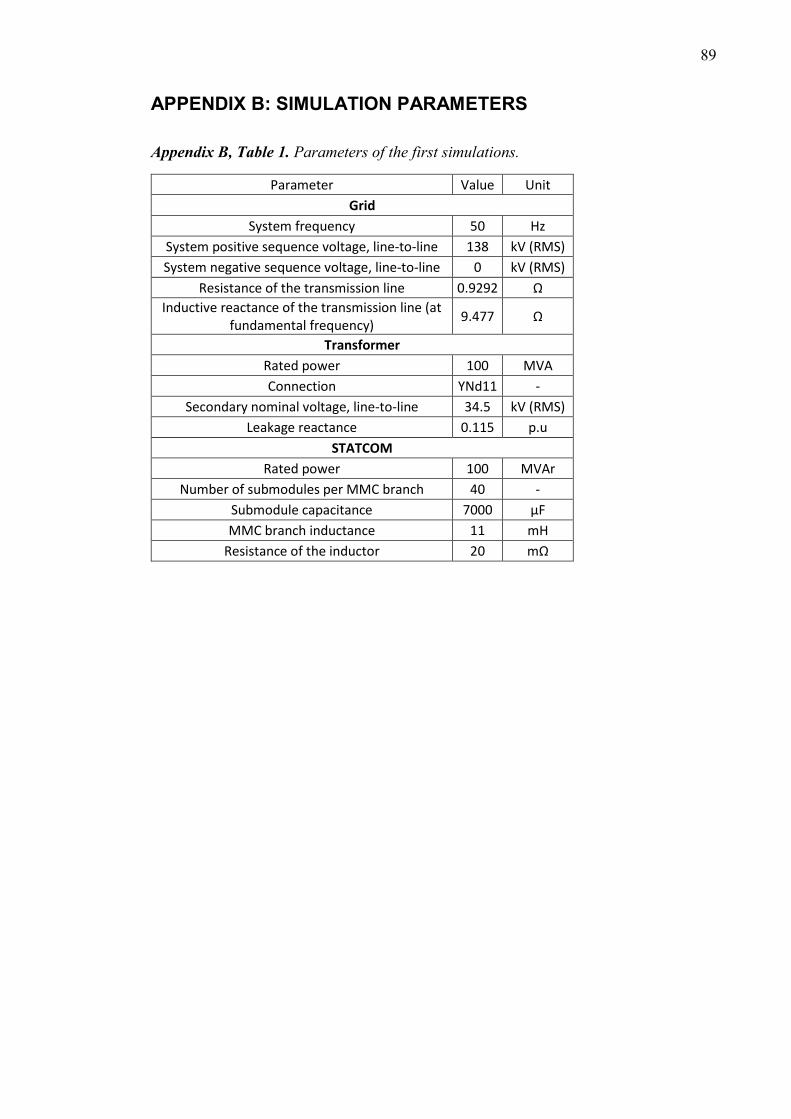
89

APPENDIX B: SIMULATION PARAMETERS

Appendix B, Table 1. Parameters of the first simulations.

Parameter Value Unit

Grid

System frequency 50 Hz

System positive sequence voltage, line-to-line 138 kV (RMS)

System negative sequence voltage, line-to-line 0 kV (RMS)

Resistance of the transmission line 0.9292 Ω

Inductive reactance of the transmission line (at fundamental frequency)

9.477 Ω

Transformer

Rated power 100 MVA

Connection YNd11 -

Secondary nominal voltage, line-to-line 34.5 kV (RMS)

Leakage reactance 0.115 p.u

STATCOM

Rated power 100 MVAr

Number of submodules per MMC branch 40 -

Submodule capacitance 7000 μF

MMC branch inductance 11 mH

Resistance of the inductor 20 mΩ