power laws and scaling of rain events and · pdf filethe concept of self-organized criticality...

POWER LAWS AND SCALING OF RAIN EVENTS AND DRY

SPELLS IN THE CATALONIA REGION

ANNA DELUCA AND ALVARO CORRAL

Abstract. We analyze the statistics of rain-event sizes, rain-event durations, anddry-spell durations in a network of 20 rain gauges scattered in an area situated closeto the NW Mediterranean coast. Power-law distributions emerge clearly for the dry-spell durations, with an exponent around 1.50 ± 0.05, although for event sizes anddurations the power-law ranges are rather limited, in some cases. Deviations frompower-law behavior are attributed to finite-size effects. A scaling analysis helps toelucidate the situation, providing support for the existence of scale invariance in thesedistributions. It is remarkable that rain data of not very high resolution yield findingsin agreement with self-organized critical phenomena.

1. Introduction

The concept of self-organized criticality (SOC) aims for explaining the origin ofpower-law distributed event sizes in a broad variety of systems [1, 2, 3, 4]. Indeed,it has been found that for diverse phenomena that take place in terms of bursts ofactivity interrupting larger quiet periods, the size s of these bursty episodes or eventsfollows a power-law distribution,

(1) Ps(s) ∝1

sτs,

over a certain range of s, with Ps(s) the probability density of the event size and τs itsexponent (and the sign ∝ indicating proportionality).

The paradigmatic example of this behavior is a sandpile that is perturbed by theslow addition of extra grains: most of the time the activity in the pile is negligible,but at some instant a new added grain triggers an instability that propagates throughthe system in the form of an avalanche; these are the high-activity periods whose sizeis power-law distributed; the avalanche size can be measured from the dissipation ofenergy, as the change in potential energy before and after the event, for example [5].

Power-law distributions signal the absence of characteristic scales [4, 6]. The mainidea behind SOC is the recognition that such scale invariance in event sizes is achievedbecause of the existence of a nonequilibrium continuous phase transition whose criticalpoint is an attractor of the dynamics [7, 8, 9]. When the system settles at the criticalpoint, scale invariance and power-law behavior is ensured, as these peculiarities are thedefining characteristics of critical phenomena [4]. (Notice that from this point of view,SOC is just a suggestion for the origin of scale invariance, other mechanism can leadto the same observable results [3].)

1

POWER LAWS AND SCALING OF RAIN EVENTS AND DRY SPELLS IN CATALONIA 2

Although the original idea of SOC was inspired mainly by a variety of systemsin condensed-matter physics [10], the concept has been particularly fruitful in thegeosciences, with a special impact in natural hazards. Indeed, earthquakes [1, 11],landslides and rock avalanches [12], volcanic eruptions [12, 13], forest fires [14], andeven the extinction of biological species [15], have been proposed as realizations ofSOC systems.

However, the penetration of atmospheric science by SOC has been much more mod-est. As far as we know, the pioneering papers are those of [16] and Peters et al.[17, 18, 19], who studied rainfall as an avalanche process. Both authors dealt with lo-cally measured precipitation and defined, independently, a rain event as the sequenceof rain occurrence for which the rain rate (i.e., the activity) is always greater than zero.Then, the focus of the SOC approach is not on the total amount of rain recorded in afixed time period (for instance, one day, or one month), but on the rain event, which iswhat defines in each case the time period of rain-amount integration. In this way, theevent size is the total amount of rain collected during the duration of the event. We canrecognize a contraposition between the anthropogenic perspective, paying attention torain over relatively large time periods, and a more physical approach, looking at thefine structure of the rainfall phenomenon [18].

The analysis of Andrade et al. considered long-term daily rain records from severalweather stations in Brazil, India, Europe, and Australia, with observation times rangingfrom a dozen years up to more than a century. The rain rate was taking values between0.1 mm/day to about 100 mm/day. Although the dry spell (the time between rainevents) seemed to follow a steep power-law distribution (at least for some stations insemi-arid regions), the rain-event size was not reported, and therefore the possibleconnection between SOC and rainfall could not be really checked.

On the other hand, Peters et al. used in their study a totally different dataset,obtained from the operation of a vertically pointing Doppler radar situated in theBaltic coast of Germany. This facility provided rain rates at an altitude between 250m and 300 m above sea level, covering an area of 70 m2, with a detection threshold equalto 0.005 mm/hour at a one-minute temporal resolution. The time period analyzed wasfrom January to July 1999. A power-law event-size distribution was obtained for sbetween about 0.01 mm and 30 mm, with an exponent τs ≃ 1.4. Dry-spell durationsalso seemed to follow a power-law distribution between 5 min and 4 days (roughly),with an exponent τq ≃ 1.4, but superimposed to a daily peak. For the event-durationdistribution the behavior was not so clear, although a power law with an exponentτd ≃ 1.6 could be fit to the data. In any case, the clean power-law behavior obtainedfor the distributions of event sizes allowed to establish a patent parallelism betweenrainfall and SOC phenomena [19].

A radically different approach was followed by [20]. Instead of addressing theirattention to the event-size distribution and looking for a power-law behavior (as inthe overwhelming majority of SOC studies), they analyzed, from the Tropical RainfallMeasuring Mission, satellite microwave estimates of rain rate and vertically integrated(i.e., column) water vapour content in grid points covering the tropical oceans (with a


0.25◦ spatial resolution in latitude and longitude). The results were not only interestingas a support of SOC ideas but also for the characterization of rainfall phenomena andthe problem of atmospheric convection. They showed a relationship between the twovariables in the form of a sharp increase of the rain rate when a threshold value of thewater vapor was reached, analogous to what is obtained in critical phase transitions.Moreover, these authors also demonstrated that most of the time the state of thesystem was close to the transition point (i.e., most of the measurements of the watervapor correspond to values near the critical one), providing perhaps the first directobservational support of the applicability of SOC theory to the natural world. Further,they connected these ideas with the classical concept of atmospheric quasi-equilibriumproposed by Arakawa and Schubert around 35 years ago [21].

In summary, the question of the existence of SOC in rainfall is far from being totallysolved. Power-law size distributions allow a connection to be established: if SOCsystems show distributions that are power law, and the system under study displays apower-law distribution, there exists the possibility that the system is a SOC system,although alternative mechanisms could explain the power law [3, 22]. In any case, thework of [16] resulted inconclusive in terms of establishing a link between rainfall andSOC, whereas the positive power-law findings of [17] could be considered somewhat“incidental”, as it was based in a single dataset from a mid-latitude region.

In contrast, the key findings of Peters and Neelin suggest the existence of an at-tractive critical point in the rainfall transition over the tropical oceans, but curiously,the most common “test” for SOC, the construction of the event-size distribution, hasbarely been applied to tropical precipitation records (but see [23]). The goal of thispaper is to contribute to extend the evidence for SOC in rainfall, studying a climatol-ogy that can be considered as a link between the Baltic-sea case analyzed by Peterset al. and the tropical oceans of Peters and Neelin. With this purpose, we performan in-depth analysis of local (i.e., zero-dimensional) rainfall records in Catalonia, arepresentative region of the Northwestern Mediterranean. Indeed, we can view rainfallthere as something in between the Baltic rain and the tropical convection, dominatedby frontal systems during the Winter and mainly of convective origin in the Sum-mer. Additionally, as a by-product of our study, we obtain a complete characterizationof rain in the Catalonia region, which we consider generalizable to the NorthwesternMediterranean. A much broader study, covering very different climates and using raindata with higher resolution will be presented in [24], in order to verify the universalityof rain-event statistics.

Note that the presence of SOC in rainfall has important consequences for the risksposed by this natural phenomenon. If there is not a characteristic rain-event size, thenthere is neither a definite separation nor a fundamental difference between the smallestharmless rains and the most hazardous storms. Further, the critical evolution of therain events suggests that, at a given instant, it is equally likely that the rain rateintensifies or decreases, the outcome depending on a myriad of uncontrollable details,which makes detailed prediction unattainable in practice [25]. Our findings imply thatthis is the case for Mediterranean storms.


Figure 1. Map showing the position of the rain gauges analyzed acrossCatalonia. The location of the region in the NW of the Mediter-ranean is also shown. (Coast lines and old political borders taken fromhttp://rimmer.ngdc.noaa.gov/coast.)

2. Data

We have analyzed 20 stations in Catalonia (NE Spain) from the database maintainedby the Agencia Catalana de l’Aigua (ACA, http://aca-web.gencat.cat/aca). Thesedata come from a network of rain gauges, called SICAT (Sistema Integral del Cicle del’Aigua al Territori, formerly SAIH, Sistema Automatic d’Informacio Hidrologica); partof the stations belong to the ACA and the rest to the Servei Meteorologic de Catalunya,and they are used to monitor the state of the inland drainage basins of this region. Theinland basins are those comprising the rivers which are born and die in the Catalanterritory [26]. The corresponding sites are listed in Table 1, together with their latitudeand longitude; a map is also provided in Fig. 1. All datasets cover a time period startingon January 1st, 2000, at 0:00, and ending either on June 30th or on July 1st, 2009(spanning roughly 9.5 years), except the Cap de Creus one, which ends on June 19th,2009 (this is just a 0.35 % relative difference in record length). The same database,although for a different time period, was also used in [26].

In all the stations, rain is measured by the same weighing precipitation gauge, thedevice called Pluvio from OTT (http://www.ott-hydrometry.de), either with a ca-pacity of 250 or 1000 mm and working through the balance principle. It measuresboth liquid or/and solid precipitation. The precipitation rate is recorded in intervalsof ∆t = 5 min, with a resolution of 1.2 mm/hour (which corresponds to 0.1 mm in 5min). This precipitation rate can be converted into an energy flux through the latentheat of condensation of water, which yields 1 mm/hour ≃ 690 W/m2 (this is abouthalf the value of the solar constant). An example of a complete record is provided inFig. 2 for the site of Muga.


Table 1. Characteristics of all the sites for the 9-year period 2000-2008.Every site is named by the corresponding river basin or subbasin, the mu-nicipality is included only in ambiguous cases. Ll. stands for Llobregatriver. fM is the fraction of missing records (time missing divided bytotal time); fD is the fraction of discarded times; fr is the fraction ofrainy time (time with r > c divided by total undiscarded time, for atime resolution ∆t = 5 min); a. rate is the annual rain rate, calculatedonly over undiscarded times; c. rate is the rain rate conditioned to rain,i.e., calculated over the (undiscarded) rainy time; Ns is the number ofrain events and Nq the number of dry spells; the rest of symbols areexplained in the text. The differences between Ns and Nq are due to themissing records. Sites are ordered by increasing annual rate. The tableshows a positive correlation between fr, the annual rate, Ns and Nq, andthat these variables are negatively correlated with 〈q〉 and 〈q2〉 / 〈q〉. Incontrast, the rate conditioned to rain is roughly constant, taking valuesbetween 3.3 and 3.8 mm/hour.

site longitude latitude fM fD fr a. rate c. rate Ns Nq 〈s〉〈s2〉〈s〉

〈d〉〈d2〉〈d〉

〈q〉〈q2〉〈q〉

E N % % % mm/yr mm/h mm mm min min min min

1 Gaia 1◦ 20’ 18” 41◦ 14’ 09” 0.08 3.71 1.6 470.9 3.3 5021 5014 0.81 11.7 14.9 92.4 894. 17958.

2 Foix 1◦ 39’ 15” 41◦ 15’ 26” 0.07 3.38 1.6 500.6 3.6 4850 4844 0.90 14.8 15.0 73.1 929. 17823.

3 Baix Ll. S.J. Despı 2◦ 02’ 52” 41◦ 21’ 13” 0.07 2.28 1.7 505.8 3.3 5374 5369 0.83 13.5 15.0 71.6 847. 16723.

4 Garraf 1◦ 41’ 39” 41◦ 13’ 55” 0.09 3.30 1.6 507.8 3.7 4722 4716 0.94 15.2 15.2 68.1 956. 15485.

5 Baix Ll. Castellbell 1◦ 51’ 34” 41◦ 38’ 54” 0.06 2.81 1.7 510.7 3.4 4950 4947 0.90 12.4 15.8 77.2 914. 16060.

6 Francolı 1◦ 10’ 51” 41◦ 21’ 60” 0.44 13.37 1.8 528.2 3.4 4539 4540 0.91 11.3 16.1 78.6 887. 13627.

7 Besos Barcelona 2◦ 12’ 06” 41◦ 27’ 09” 0.15 4.17 1.7 531.8 3.5 4808 4803 0.95 12.1 16.2 70.5 928. 18617.

8 Riera de La Bisbal 1◦ 32’ 15” 41◦ 12’ 53” 0.07 3.66 1.6 540.0 3.8 4730 4724 0.99 13.8 15.8 75.2 950. 18334.

9 Besos Castellar 2◦ 04’ 57” 41◦ 36’ 37” 4.34 13.59 2.0 633.3 3.6 4918 4970 1.00 11.6 16.9 79.5 806. 17276.

10 Ll. Cardener 1◦ 35’ 14” 42◦ 06’ 14” 0.07 3.33 2.1 652.4 3.5 6204 6197 0.92 10.0 15.7 68.6 723. 13986.

11 Ridaura 2◦ 58’ 49” 41◦ 49’ 12” 0.12 2.41 2.0 674.2 3.8 5780 5774 1.02 19.3 16.1 87.7 784. 12702.

12 Daro 3◦ 02’ 22” 41◦ 57’ 59” 0.06 2.09 2.2 684.5 3.6 5553 5547 1.09 16.9 18.0 109.2 818. 14054.

13 Tordera 2◦ 40’ 14” 41◦ 44’ 50” 0.08 2.04 2.3 688.8 3.4 7980 7977 0.76 14.1 13.6 93.2 568. 11999.

14 Baix Ter 2◦ 49’ 32” 41◦ 58’ 37” 0.07 2.71 2.3 710.2 3.6 6042 6036 1.03 16.4 17.4 104.7 746. 12949.

15 Cap de Creus 3◦ 07’ 35” 42◦ 25’ 40” 0.07 2.92 2.3 741.5 3.7 5962 5955 1.09 22.6 17.7 123.3 754. 13864.

16 Alt Llobregat 1◦ 52’ 15” 42◦ 12’ 58” 3.12 5.82 2.6 742.8 3.3 6970 6988 0.90 11.0 16.7 87.9 621. 10675.

17 Muga 2◦ 50’ 10” 42◦ 20’ 42” 0.06 2.56 2.4 749.3 3.6 6462 6457 1.02 31.5 16.9 119.4 698. 11415.

18 Alt Ter Sau 2◦ 24’ 53” 41◦ 58’ 14” 0.08 2.43 2.5 772.1 3.6 6966 6961 0.97 15.2 16.3 112.6 647. 11292.

19 Fluvia 2◦ 57’ 20” 42◦ 09’ 20” 3.09 4.74 2.3 772.4 3.8 6287 6319 1.05 19.0 16.7 99.6 697. 8881.

20 Alt Ter S. Joan 2◦ 14’ 38” 42◦ 13’ 25” 0.07 1.98 2.8 795.1 3.3 8333 8327 0.84 11.4 15.5 91.1 542. 7260.

In order to make the datasets more manageable, zero-rain rates are reported onlyevery hour. This leads us to infer that time intervals larger than 1 hour have to beconsidered as operational errors. The ratio of these missing times to the total timecovered in the record is denoted as fM in Table 1, where it can be seen that this ratiois usually below 0.1 %. However, there are 3 cases in which its value is around 3 or4 %. Other quantities reported in the table are the fraction of time corresponding to


1

10

100

2000 2001 2002 2003 2004 2005 2006 2007 2008 2009

r (mm/h)

t (years)

Figure 2. Evolution of the rate in the Muga site for the 9.5 yearsspanned by the record.

rain, fr, the annual mean rate, and the mean rate conditioned to rain periods. Notethat for a fractal point process a quantity as fr only makes sense for a concrete timeresolution, in our case, ∆t = 5 min.

3. Analysis and Results

3.1. Rain events and dry spells. As we have mentioned in the first section, the keyof our analysis is the rain event [16, 17]. If r(t) denotes the rain rate at discrete time t(in intervals of 5 minutes in our case), a rain event is defined by the sequence of rates{r(tn), r(tn+1), . . . r(tm)} such that r(ti) > c for i = n, n + 1, . . . m, but with r(ti) ≤ cfor i = n − 1 and i = m + 1. In words: a rain event starts when the threshold c issurpassed, all the rates in the event are above the threshold, and it ends when the ratecrosses the threshold from above. In this paper we have considered c = 0, which, dueto the resolution of the record, is equivalent to take c → 1.2− mm/hour (where thesuperscript means that we are just below the value 1.2).

A quantity of interest is the duration d of the event, which is the time period coveredby the sequence of above-threshold rates, i.e., d ≡ tm − tn + ∆t; note that this is amultiple of ∆t = 5 min. Even more relevant it is to consider the size of the event,which is defined as the total rain collected during the event,

s ≡m

∑

i=n

r(ti)∆t ≃∫ tm

tn

r(t)dt;

it is measured in mm and it is always a multiple of 0.1 mm (1.2 mm/hour × 5 min).The event size is proportional, through the latent heat of condensation, to the energy


0

20

40

60

80

100

4 5 6 7 8 9 10 11

r (mm/h)

t (h)

Figure 3. Time evolution of the rate of the rain event with the largestsize in the Muga site. This event took place on April 11, 2002, and isalso the largest (in size) of all sites, with s = 248.7 mm. Time refersto hours since midnight. A very small rain event is also present at thebeginning, with s = 0.3 mm and separated to the main event by a dryspell of duration q = 15 min.

released by the event per unit area, with 1 mm ≃ 2500 kJ/m2 [24], and can be con-sidered a measure of energy dissipation, as is done for SOC systems. Figure 3 showsas an illustration the evolution of the rate for the largest event in the record, whichhappens at the Muga site, whereas Fig. 4(a) displays the sequence of all events in thesame site. Figure 4(b) shows the size of all events in Muga as a function of their du-ration, with considerable resemblance to [27]. Further, the dry spells are the periodsbetween consecutive rain events (then, they verify r(t) ≤ c). If the last record of anevent is at tm and the next event starts at the interval t = tp, the dry-spell duration isq ≡ tp − tm − ∆t, which is also a multiple of 5 min.

When a rain event, or a dry spell, is interrupted due to missing data, we discard thatevent or dry spell, and count the recorded duration as discarded time; the fraction ofthese times in the record appears in Table 1, under the symbol fD. Although in somecases the duration of the interrupted event or dry spell can be bounded from below orfrom above, we have not attempted that estimation.

3.2. Rain-event and dry-spell probability densities. Due to the enormous vari-ability of the 3 quantities just defined, the most informative approach is to work withtheir probability distributions. Taking the size as an example, its probability densityPs(s) is defined as the probability that the size is between s and s + ds divided byds, with ds → 0. Then,

∫ ∞

0Ps(s)ds = 1. This implicitly assumes that s is consid-

ered as a continuous variable (but see below). Note that the annual number densities


0.1

1

10

100

1000

2000 2001 2002 2003 2004 2005 2006 2007 2008 2009

s (mm)

t (years)

10-1

100

101

102

100

101

102

103

s (m

m)

d (min)

Figure 4. (a) Size of all rain events versus their occurrence time in theMuga site. (b) Size of all rain events as a function of their duration inthe same site. Note that the event with the largest size is not the longestone.

[17, 18, 19] are trivially recovered multiplying the probability densities by the totalnumber of events and dividing by total time.

In practice, the estimation of the density from data is performed taking a valueof ds large enough to guarantee statistical significance, and then compute Ps(s) asn(s)/(Ns∆), where n(s) is the number of events with size in the range between s ands + ds, Ns the total number of events, and ∆ is defined as ∆ = Rs(⌊(s + ds)/Rs⌋ −⌊s/Rs⌋), with Rs the resolution of s, i.e. Rs = 0.1 mm, and ⌊x⌋ the integer part ofx (but note that high resolution means low Rs). So, ∆/Rs is the number of possibledifferent values of the variable in the interval considered. Notice that using ∆ insteadof ds in the denominator of the estimation of Ps(s) allows one to take into account the


discreteness of s. If Rs tended to zero, then ∆ → ds and the discreteness effects wouldbecome irrelevant.

How large does ds have to be to guarantee the statistical significance of the estimationof Ps(s)? Working with long-tailed distributions (where the variable covers a broadrange of scales) a very useful procedure is to take a width of the interval ds that isnot the same for all s, but that is proportional to the scale, as [s, s + ds) = [so, bso),[bso, b

2so), . . . [bkso, bk+1so), i.e., ds = (b − 1)s (with b > 1). Given a value of s, the

corresponding value of k that associates s with its bin is given by k = ⌊logb(s/so)⌋.Correspondingly, the optimum choice to assign a point to the interval [s, s + ds) is

given by the value√

bs. This procedure is referred to as logarithmic binning, becausethe intervals appear with fixed width in logarithmic scale [28]. In this paper we havegenerally taken b ≃ 1.58, in such a way that b5 = 10, providing 5 bins per order ofmagnitude.

As the distributions are estimated from a finite number of data, they display statis-tical fluctuations. The uncertainty characterizing these fluctuations is simply relatedto the density by

σD(s)

Ps(s)≃ 1

√

n(s),

where σD(s) is the standard deviation of Ps(s) (do not confound with the standarddeviation of s). This is so because n(s) can be considered a binomial variable [29],and then, the ratio between its standard deviation and mean fulfills σn(s)/〈n(s)〉 =√

Nsp(1 − p)/(Nsp) ≃√

(1 − p)/n(s) ≃ 1/√

n(s), with n(s) ≃ pNs and p ≪ 1. AsPs(s) is proportional to n(s), the same relation holds for its relative uncertainty.

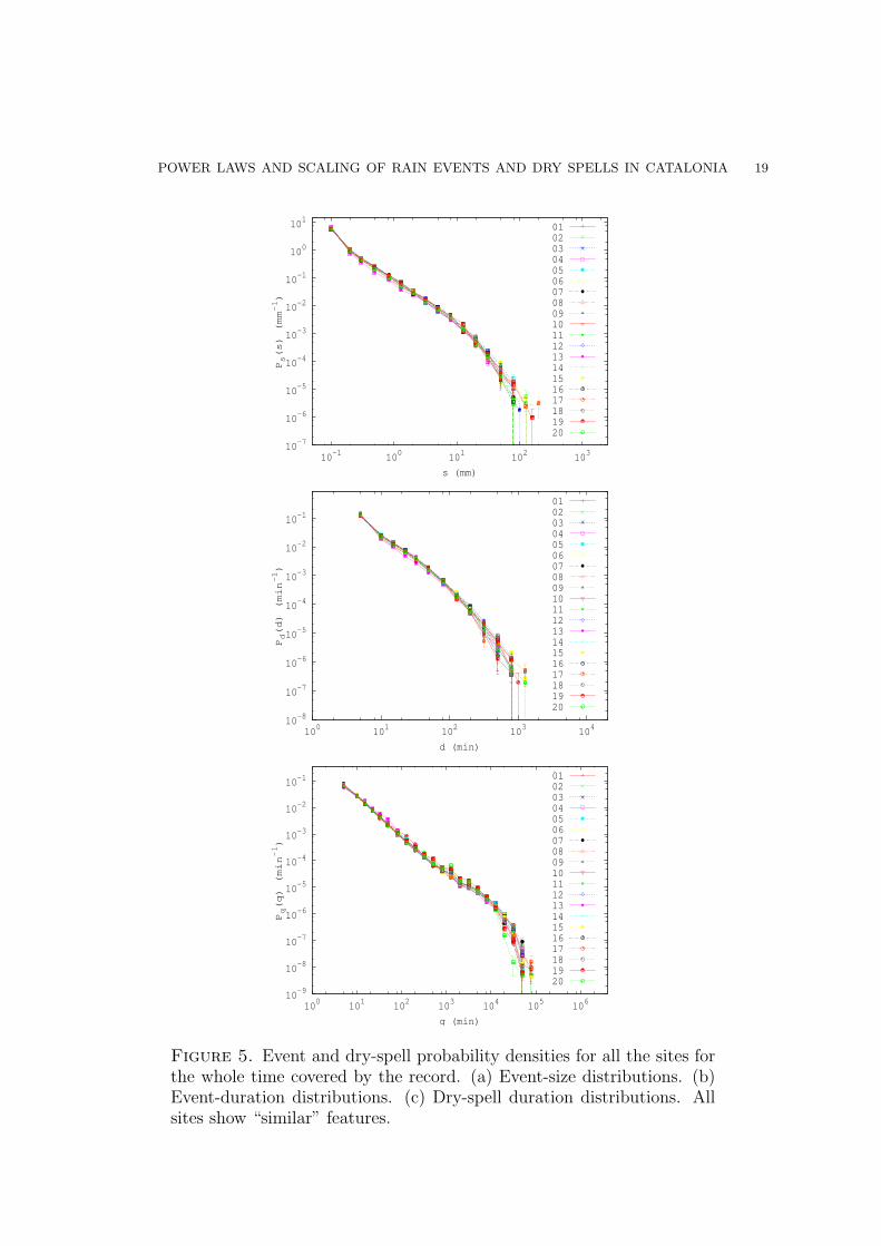
The results for the probability densities Ps(s), Pd(d), and Pq(q) of all the sites understudy are shown in Fig. 5. In all cases the distributions show a very clear behavior,monotonically decreasing and covering a broad range of values. However, to the nakedeye, the power-law behavior necessary for SOC is not clearly apparent, in general(remember that a power law appears as a straight line in a double logarithmic plot,i.e., log Ps(s) = −τs log s + constant). Only the distribution of dry spells, Pq(q), seemsto be clearly linear between certain values of q. Moreover, these are the broadestdistributions, covering a range of more than 4 orders of magnitude, from 5 min toabout a couple of months. In addition, a daily peak seems to be present in somesites (1 day = 1440 min), as in [17]. In the opposite side we find the distributions ofdurations, Pd(d), whose range is the shortest, from 5 min to about 1 day (two and a halfdecades), and for which no straight line is visible in the plot; rather, the distributionsappear as convex. The size distributions Ps(s) are somehow in between, defined forabout 3 orders of magnitude (from 0.1 to 200 mm roughly) and perhaps with a shortrange of power-law behavior.

3.3. Fitting and testing power laws. A quantitative method can put more rigorinto these observations. The idea is based on the recipe proposed by [30], but gener-alized to our problem. Essentially, an objective procedure is required in order to findthe optimum range in which a power law may hold. Taking again the event size for


illustration, we report the power-law exponent fit between the values of smin and smax

which yield the maximum number of data in that range but with a p−value greaterthan 10%. The method is described in detail in [24], but we summarize it in the nextparagraphs.

For a given value of the pair smin and smax, the maximum-likelihood (ML) power-lawexponent is estimated for the events whose size lies in that range. This exponent yieldsa fit of the distribution, and the goodness of such a fit is evaluated by means of theKolmogorov-Smirnov (KS) test [31]. The purpose is to get a p−value, which is theprobability that the KS test gives a distance between true power law data and its fitlarger than the distance obtained between the empirical data and its fit.

For instance, p = 20% would mean that truly power-law distributed data were closerthan the empirical data to their respective fits in 80% of the cases, but in the rest 20%of the cases a true power law were at a larger distance than the empirical data. So, insuch a case the KS distance turns out to be somewhat large, but not large enough toreject that the data follow a power law with the ML exponent.

As in the case in which some parameter is estimated from the data there is noclosed formula to calculate the p−value, we perform Monte Carlo simulations in orderto compute the statistics of the Kolmogorov-Smirnov distance and from there thep−value. In this way, for each smin and smax we get a number of data in that range anda p−value. We look for the values of the extremes (smin and smax) which maximize thenumber of data in between but with the restriction that the p−value has to be greaterthan 10% (this threshold is arbitrary, but the conclusions do not change if it is moved).The maximization is performed sweeping 100 values of smin and 100 values of smax, inlog-scale, in such a way that all possible ranges (within this log-resolution) are takeninto account. We have to remark that, in contrast with [24], we have considered alwaysdiscrete probability distributions, both in the ML fit and in the simulations. Noticealso that the method is not based on the estimation of the probability densities shownin the previous subsections.

The results of this method are in agreement with the visual conclusions obtained inthe previous subsection, as can be seen in Table 2. Starting with the size statistics, 13out of the 20 sites yield reasonable results, with an exponent τs between 1.43 and 1.54over a logarithmic range smax/smin from 12 to more than 200. For the rest of the sites,the range is too short (less than one decade). In the application of the algorithm, ithas been necessary to restrict the value of smin to be smin ≥ 0.2 mm; otherwise, as thedistributions have a concave shape (in logscale) close to the origin (which means thatthere are many more events in that scale than at larger scales), the algorithm (whichmaximizes the number of data in a given range) prefers a short range with many dataclose to the origin than a larger range with less data away from the origin. Perhaps avariation of the algorithm in which the quantity that is maximized is the logarithmicrange would not need this restriction.

For the distribution of durations the results are worse, as expected (worse in thesense that the power-law fit is worse than in the previous case). Only 4 sites do notgive totally unacceptable results, with τd ranging from 1.66 to 1.74 and dmax/dmin from


6 to 12. The other sites yield too short ranges for the power law be of any relevance.The situation is analogous to the case of the distribution of sizes, but the resultingranges are much shorter here [24]. Notice that the excess of events with d = 5 min,eliminated from the fits imposing dmin ≥ 10 min, has no counterpart in the value ofthe smallest rate (not shown), and therefore, this extra number of events is probablydue to problems in the time resolution of the data.

Considerably better are the results for the dry spells. 16 sites give consistent results,with τq from 1.45 to 1.55 in a range qmax/qmin from 30 to almost 300. It is noticeablethat in these cases qmax is always below 1 day. Perhaps, the removal by hand of dryspells around that value could enlarge a little the power-law range. In the rest ofsites, either the range is comparatively too short (for example, for the Gaia site, thepower-law behavior of Pq(q) is interrupted at around q = 100 min), or the algorithmhas a tendency to include the bump the distributions show between the daily peak (qbeyond 1000 min) and the tail. This makes the value of the exponent smaller.

In summary, the best power laws for the distributions of durations are too short tobe relevant, and the fits for the sizes are in the limit of what is acceptable or not (somecases are clear and some other not). Only the distributions of dry spells give reallygood power laws (with τq = 1.50 ± 0.05, and for more than two decades in 6 sites).

3.4. Non-parametric scaling. Nevertheless, the fact that a power-law behavior doesnot exist over a broad range of values does not rule out the existence of SOC [4]. Infact, the fulfillment of a power-law distribution in the form of Eq. (1) is only validwhen finite-size effects are “small”, which only happens for large enough systems. Ingeneral, when these effects are taken into account, SOC behavior leads to distributionsof the form [4, 24]

(2) Ps(s) = s−τsGs(s/sξ) for s > sl,

where Gs(x) is a scaling function that is essentially constant for x < 1 and decays fastfor x > 1, accounting in this way for the finite-size effects when s is above the crossovervalue sξ; the size sl is just a lower cutoff limiting the validity of this description. Noticethat for a power-law behavior to hold over an appreciable range, it is necessary that thescales given by sl and sξ are well separated, i.e., sl ≪ sξ. As sξ increases with systemsize, typically as sξ ∝ LDs (with Ds the so-called avalanche dimension, or event-sizedimension), the power-law condition (1) can only be fulfilled for large enough systemsizes.

However, it is not clear what the system size L is for rainfall. May it be the verticalextension of the clouds, or the depth of the troposphere? In any case, we do not needto bother about its definition since, whatever it is, it is not accessible to us (rememberthat all our data are just local rain rates). Nevertheless, the scaling ansatz (2) still canbe checked from data. First, notice that the ansatz implies that the k−order momentof s scale with L as

(3) 〈sk〉 ∝ LDs(k+1−τs) for 1 < τs < k + 1,


Table 2. Results of the power-law fitting and goodness-of-fit tests ap-plied to event sizes, event durations, and drought durations, for the pe-riod of 9 and a half years specified in the main text. The table displaysthe minimum and maximum fitting range, the ratio of these values (loga-rithmic range), total number of events, number of events in fitting range(Ns, Nd, and Nq, for s, d, and q, respectively), and the power-law expo-nent with its uncertainty (one standard deviation) calculated as stated by[32] and displayed between parenthesis as the variation of the last digit.All the fits have a p−value larger than 10 %. The results of [18], labeledas ChP, are also included, the fitting ranges are estimated visually fromtheir plots.

site smin smaxsmax

smin

Ns Ns τs

mm mm

1 0.2 36.1 180.5 5393 1886 1.54(2)

2 0.2 0.9 4.5 5236 1323 1.64(6)

3 0.2 31.1 155.5 5749 2111 1.53(2)

4 0.2 2.4 12.0 5108 1745 1.43(3)

5 0.2 28.0 140.0 5289 2106 1.52(2)

6 0.2 13.6 68.0 4924 1969 1.49(2)

7 0.2 21.1 105.5 5219 2234 1.51(2)

8 0.2 42.6 213.0 5112 2047 1.53(2)

9 0.2 1.0 5.0 5366 1459 1.53(5)

10 0.2 3.8 19.0 6691 2452 1.51(2)

11 0.2 13.0 65.0 6224 2373 1.49(2)

12 0.2 0.8 4.0 5967 1500 1.53(6)

13 0.3 20.0 66.7 8330 1853 1.45(2)

14 0.2 0.7 3.5 6525 1711 1.56(6)

15 0.3 1.1 3.7 6485 1102 1.39(7)

16 0.2 0.7 3.5 7491 1852 1.59(5)

17 0.2 16.1 80.5 6962 2853 1.52(2)

18 0.2 8.3 41.5 7511 2847 1.51(2)

19 0.2 19.9 99.5 6767 2742 1.47(2)

20 0.2 0.7 3.5 9012 2047 1.69(5)

ChP 0.01 30 300 – – 1.4

dmin dmaxdmax

dmin

Nd τd

min min

10 100 10.0 1668 1.67(4)

10 40 4.0 1581 1.60(6)

10 60 6.0 1726 1.66(5)

10 35 3.5 1564 1.41(7)

10 35 3.5 1530 1.58(7)

10 35 3.5 1441 1.59(7)

10 35 3.5 1621 1.51(7)

10 40 4.0 1567 1.55(6)

10 40 4.0 1658 1.51(6)

10 35 3.5 2066 1.57(6)

10 50 5.0 1932 1.56(5)

10 40 4.0 1889 1.49(6)

10 125 12.5 2288 1.74(3)

10 50 5.0 2299 1.62(4)

10 50 5.0 2095 1.64(5)

10 40 4.0 2385 1.59(5)

10 35 3.5 2087 1.60(6)

10 35 3.5 2238 1.57(6)

10 35 3.5 1958 1.60(6)

10 85 8.5 2972 1.66(3)

10 300 30 – 1.6

qmin qmaxqmax

qmin

Nq Nq τq

min min

95 740 7.8 5387 743 1.75(7)

5 1365 273.0 5231 4729 1.46(1)

10 800 80.0 5745 3207 1.53(2)

5 980 196.0 5103 4520 1.47(1)

20 945 47.3 5287 1706 1.45(2)

20 625 31.3 4926 1537 1.47(3)

5 1280 256.0 5215 4734 1.51(1)

15 975 65.0 5107 2098 1.50(2)

10 900 90.0 5419 2889 1.55(2)

25 825 33.0 6685 1758 1.48(3)

45 21075 468.3 6219 2005 1.24(1)

5 1175 235.0 5961 5376 1.47(1)

130 20600 158.5 8328 1501 1.27(2)

5 1075 215.0 6520 5906 1.47(1)

15 745 49.7 6479 2560 1.51(2)

5 1070 214.0 7510 6789 1.50(1)

10 685 68.5 6958 3719 1.52(1)

20 620 31.0 7507 2302 1.53(2)

50 1085 21.7 6800 1378 1.26(3)

15 515 34.3 9007 3367 1.50(2)

5 ∗6000 1200 – – 1.4∗ Disregarding the daily peak.

if sl ≪ sξ, see [4]. Second, Eq. (2) can be written in a slightly different form, as ascaling law,

(4) Ps(s) = L−DsτsFs(s/LDs) for s > sl,

where the new scaling function Fs(x) is defined as Fs(x) ≡ x−τsGs(x/a) (a is theconstant of proportionality between sξ and LDs). This form of Ps(s) (in fact, Ps(s, L)),with an arbitrary F , is the well-known scale-invariance condition [4, 6]. Changes ofscale (linear transformations) in s and L may leave the shape of the function Ps(s, L)unchanged (this is what scale invariance means, power laws are just a particular case).


Substituting LDs ∝ 〈s2〉 / 〈s〉 and LDsτs ∝ L2Ds/ 〈s〉 ∝ 〈s2〉2 / 〈s〉3 (from the scalingof

⟨

sk⟩

, assuming τs < 2) into Eq. (4) leads to

(5) Ps(s) = 〈s〉3⟨

s2⟩−2 Fs(s 〈s〉 /

⟨

s2⟩

)

where Fs(x) is essentially the scaling function Fs(x), absorbing the proportionality

constants. Therefore, if scaling holds, a plot of 〈s2〉2 Ps(s)/ 〈s〉3 versus s 〈s〉 / 〈s2〉 forall the sites has to yield a collapse of the distributions into a single curve, which drawsFs(x) (a similar procedure is outlined in [33]). In order to proceed, the mean and thequadratic mean, 〈s〉 and 〈s2〉, can be easily estimated from data. These values, andthe corresponding ones for d and q are displayed for all sites in Table 1.

The outcome for Ps(s), Pd(d), and Pq(q) is shown in Fig. 6, with reasonable results,especially for the distribution of dry spells. In this case, the plot suggests that thescaling function Gq(x) has a maximum around x ≃ 1, but this does not invalidate ourapproach, which assumed constant Gq(x) for small x and a fast decay for large x.

Note that the quotient 〈s2〉 / 〈s〉 gives the scale for the crossover value sξ (as sξ ∝〈s2〉 / 〈s〉, with a constant of proportionality that depends on the scaling function Gs

and on sl/sξ), and therefore it is the ratio of the second moment to the mean and notthe mean which describes the scaling behavior of the distribution. For the case of eventsizes, we get values of 〈s2〉 / 〈s〉 between 10 and 30 mm (see Table 1), and therefore thecondition sl ≪ sξ is very well fulfilled (assuming that the moment ratio 〈s2〉 / 〈s〉 is ofthe same order as sξ), which is a test for the consistency of our approach. For dry spells〈q2〉 / 〈q〉 is between 5 and 13 days, which is even better for the applicability of thescaling analysis. The case of the event durations is somewhat “critical”, with 〈d2〉 / 〈d〉between 70 and 120 min, which yields dξ/dl in the range from 14 to 24. Nevertheless,we observe that the condition sl ≪ sξ for the power law to show up is stronger thanthe same condition for the scaling analysis to be valid.

3.5. Parametric scaling. Further, a scaling ansatz as Eq. (2) or (4) allows an esti-mation of the exponent τs, even in the case in which a power law cannot be fit to the

data. From the scaling of the moments of s we get, taking k = 1, LDs ∝ 〈s〉1/(2−τs) and

LDsτs ∝ 〈s〉τs/(2−τs) (again with τs < 2); so, substituting into Eq. (4),

(6) Ps(s) = 〈s〉−τs/(2−τs) Fs(s/ 〈s〉1/(2−τs)).

One only needs to find the value of τs that optimizes the collapse of all the distributions,i.e., that makes the previous equation valid, or at least as close to validity as possible.

We therefore need a measurement to quantify distance between rescaled distribu-tions. In order to do that, we have chosen to work with the cumulative distributionfunction, Ss(s) ≡

∫ ∞

sPs(s

′)ds′, rather than with the density (to be rigorous, Ss(s)is the complementary of the cumulative distribution function, and is called survivorfunction or reliability function in some contexts). The reason to work with Ss(s) isdouble: the estimation of the cumulative distribution function does not depend of anarbitrarily selected bin width ds [31], and it does not give equal weight to all scales


in the representation of the function (i.e., in the number of points that constitute thefunction). The scaling laws (4) and (6) turn out to be, then,

(7) Ss(s) = L−Ds(τs−1)Hs(s/LDs),

(8) Ss(s) = 〈s〉−(τs−1)/(2−τs) Hs(s/ 〈s〉1/(2−τs)),

with Hs(x) and Hs(x) the corresponding scaling functions.The first step of the method of collapse is to merge all the pairs {s, Ss(s)}i into a

unique rescaled function {x, y}. If i = 1, . . . , 20 runs for all sites, and j = 1, . . . ,Ms(i)for all the different values that the size of events takes on site i (note that Ms(i) ≤Ns(i)), then,

xℓ(τ) ≡ log(sji/ 〈s〉1/(2−τ)i ),

yℓ(τ) ≡ log(Ss i(sji) 〈s〉τ/(2−τ)i ),

with sji the j-th value of the size in site i, 〈s〉i the mean on s in i, Ss i(sji) the cumulativedistribution function in i, and τ a possible value of the exponent τs. The index ℓ labelsthe new function, from 1 to

∑

∀i Ms(i), in such a way that xℓ(τ) ≤ xℓ+1(τ); i.e., thepairs xℓ(τ), yℓ(τ) are sorted by increasing x.

Then, we just compute

(9) D(τ) ≡∑

∀ℓ

(

[xℓ(τ) − xℓ+1(τ)]2 + [yℓ(τ) − yℓ+1(τ)]2)

,

which represents the sum of all Euclidean distances between the neighboring points ina (tentative) collapse plot in logarithmic scale. The value of τ which minimizes thisfunction is identified with the exponent τs in Eq. (2). We have tested the algorithmapplying it to SOC models whose exponents are well known, as the one in [34].

The results of this method applied to our datasets, not only for the size distributionsbut also to the distributions of d, are highly satisfactory. There is only one requirement:the removal of the first point in each distribution (s = 0.1 mm and d = 5 min), aswith the ML fits. The exponents we find are τs = 1.52 ± 0.12 and τd = 1.69 ± 0.01, inagreement with the ones obtained by the power-law fitting method presented above,and the corresponding rescaled plots are shown in Fig. 7. The performance of themethod is noteworthy, taking into account that the mean values of the distributionsshow little variation in most cases. In addition, the shape of the scaling function Gs can

be obtained by plotting, as suggested by Eq. (2), sτsPs(s) versus s/ 〈s〉1/(2−τs), and thesame for the other variable, d. Figure 8 displays what is obtained for each distribution.

4. Discussion and Conclusions

We have obtained evidence that rainfall in the Mediterranean region studied is com-patible with self-organized criticality. For the distributions of rain-event sizes we getpower-law exponents which are valid for at least one decade or even two in the ma-jority of sites. For the rest of the sites the fitting range is too short, but this seemsto be due to an inadequacy of the algorithm that looks for the optimum fitting range,


rather than to a real short power-law range in the data. The values of the exponents,τs ≃ 1.50±0.05, are in reasonable agreement with the value reported for the Baltic seain [17], τs ≃ 1.4, more taking into account the different nature of the data analyzed andthe disparate fitting procedures. So, we cannot rule out that the apparent agreement isa product of serendipity. For the distributions of event durations, the fitting ranges aremuch shorter, reaching in the best case one decade, although the obtained exponentsin this case, τd ≃ 1.70 ± 0.05, are compatible too with the Baltic-sea result, τd ≃ 1.6.Again, we suspect that the algorithm is the responsible for the failure in the other sites.

Nevertheless, for both observables (s and d) the range of the power laws seems ratherlimited. This is explained by the existence of finite size effects, as it is the case in other(self-organized and non-self-organized) critical phenomena. A finite-size analysis, interms of combinations of powers of the moments of the distributions, supports thisconclusion. The collapse of the distributions is a clear signature of scale-invariance:different sites share a common shape of the rain-event and dry-spell distributions, andthe only difference is in the scale of those distributions, which depends on system size.In the ideal case, in an infinite system, the power laws could then be extended withno upper cutoff. Further, the collapse of the distributions allows one an independentestimate of the power-law exponents, in surprising agreement with the values obtainedby the maximum-likelihood fit. Overall, these results are notable, in our opinion, asthey support the idea that rainfall events follow a law of dissipation analogous to theGutenberg-Richter law for earthquakes [35] and other natural hazards [12, 13, 14, 15,36], which is the hallmark of SOC systems; up to now this evidence rested essentiallyon observations in a single place [17, 18, 19, 23].

However, comparison with the new results of [24] suggests that data resolution mightplay an important role in the determination of the exponents. With a minimum de-tection rate of 0.2 mm/hour and a time resolution ∆t = 1 min it was found therethat τs ≃ 1.18, for several sites with disparate climatic characteristics, using essentiallythe same statistical techniques as in here. Better time resolution and lower detectionthreshold allow the detection of smaller events (a minimum s =0.003 mm in [24] ver-sus 0.1 mm in our case), so it is possible that we cannot see the “true” asymptotic(small s) power-law regime and that, due to the presence of the tail, we get a largervalue of the exponent. Another study with relatively poor resolution (0.1 mm/hourbut ∆t = 1hour) yielded distributions apparently compatible with τs ≃ 1.5 for smalls [37]. But one has to take also into account that a change in the detection thresholdhas a non-trivial repercussion in the size and duration of the events and the dry spells(an increase in the threshold can split one single event into two or more separate onesand vice versa). Therefore, we urge studies which explore the effects of resolution anddetection-threshold value in high-resolution rain data. (Obviously, with poor resolutiondata the detection threshold cannot be decreased, but it can be artificially increasedin very accurate data.)

On the other hand, the interpretation of the results for the distributions of dry spellsis not so clear. These distributions yield by far the best power-law fits, with exponentsin the range τq ≃ 1.50 ± 0.05 and in agreement with the previous result by [17].


However, power-law waiting times (or quiet times) between events is not a requirementfor SOC; in fact, it was previously believed that SOC avalanches happen followinga totally memoryless process, leading therefore to exponential distributions for thewaiting times. This belief has been recently denied, see for instance [38], althougha solution to this problem is not known yet. Nevertheless, in order to compare withSOC models, one would need to consider that in those cases the events are defined in aspatially extended system (in two or three dimensions), whereas our measurements aretaken in a point of the system collecting only information on the vertical scale. Thisstatement is general and should affect all the aspects of our research. Comparison with[24] shows that our value of the exponent is higher. But in this case, our power-lawrange is enough to guarantee that our estimation of the exponents are robust, and wecan only explain the discrepancy with [24] by the non-trivial effect of the change in thedetection thresholds.

In summary, we conclude that the statistics of rainfall events in the NW Mediter-ranean area studied is not essentially different to what is expected from the SOCparadigm and was confirmed essentially in one single place, up to now [24]. This con-cordance is not only qualitative but also quantitative, as only the mean rain rate isenough to characterize rain occurrence; in other words, the rain rate sets the scalearound which all events are distributed following a common shape of the probabilitydensity. This seems to indicate that SOC observables do not allow to detect climaticdifferent between regions (apart of the obvious ones given by annual rates), but shedlight on universal properties of rainfall generation. The results of this paper are veryvaluable, taking into account that the ACA network was not designed for the studyof the fine structure of rainfall; the database we use is probably in the limit of whatcan lead to detect the presence of SOC. This can motivate other researchers to lookfor SOC in intermediate-quality data, extending the evidence and the understandingof this complex phenomenon.

5. acknowledgements

This work would not have been possible without the collaboration of the AgenciaCatalana de l’Aigua (ACA), which generously shared its rain data with us. We havebenefited a lot from a long-term collaboration with Ole Peters, and are grateful also toR. Romero and A. Rosso, for addressing us towards the ACA data and an importantreference [33], and to J. E. Llebot for providing support and encouragement. Thankyou also to Joaquim Farguell from ACA. A.D. enjoys a Ph.D. grant of the Centrede Recerca Matematica. Her initial research was supported from the Explora-Ingenio2010 project FIS2007-29088-E. Other grants related to this work are FIS2009-09508and 2009SGR-164. A.C. is a participant of the CONSOLIDER i-MATH project.

References

[1] P. Bak. How Nature Works: The Science of Self-Organized Criticality. Copernicus, New York,1996.

[2] H. J. Jensen. Self-Organized Criticality. Cambridge University Press, Cambridge, 1998.


[3] D. Sornette. Critical Phenomena in Natural Sciences. Springer, Berlin, 2nd edition, 2004.[4] K. Christensen and N. R. Moloney. Complexity and Criticality. Imperial College Press, London,

2005.[5] V. Frette, K. Christensen, A. Malthe-Sørenssen, J. Feder, T. Jøssang, and P. Meakin. Avalanche

dynamics in a pile of rice. Nature, 379:49–52, 1996.[6] A. Corral. Scaling and universality in the dynamics of seismic occurrence and beyond. In

A. Carpinteri and G. Lacidogna, editors, Acoustic Emission and Critical Phenomena, pages225–244. Taylor and Francis, London, 2008.

[7] C. Tang and P. Bak. Critical exponents and scaling relations for self-organized critical phenomena.Phys. Rev. Lett., 60:2347–2350, 1988.

[8] R. Dickman, A. Vespignani, and S. Zapperi. Self-organized criticality as an absorbing-state phasetransition. Phys. Rev. E, 57:5095–5105, 1998.

[9] R. Dickman, M. A. Munoz, A. Vespignani, and S. Zapperi. Paths to self-organized criticality.Braz. J. Phys., 30:27–41, 2000.

[10] P. Bak, C. Tang, and K. Wiesenfeld. Self-organized criticality: an explanation of 1/f noise. Phys.Rev. Lett., 59:381–384, 1987.

[11] A. Sornette and D. Sornette. Self-organized criticality and earthquakes. Europhys. Lett., 9:197–202, 1989.

[12] B. D. Malamud. Tails of natural hazards. Phys. World, 17 (8):31–35, 2004.[13] F. Lahaie and J. R. Grasso. A fluid-rock interaction cellular automaton of volcano mechanics:

Application to the Piton de la Fournaise. J. Geophys. Res., 103 B:9637–9650, 1998.[14] B. D. Malamud, G. Morein, and D. L. Turcotte. Forest fires: An example of self-organized critical

behavior. Science, 281:1840–1842, 1998.[15] K. Sneppen, P. Bak, H. Flyvbjerg, and M. H. Jensen. Evolution as a self-organized critical

phenomenon. Proc. Natl. Acad. Sci. USA, 92:5209–5213, 1995.[16] R. F. S. Andrade, H. J. Schellnhuber, and M. Claussen. Analysis of rainfall records: possible

relation to self-organized criticality. Physica A, 254:557–568, 1998.[17] O. Peters, C. Hertlein, and K. Christensen. A complexity view of rainfall. Phys. Rev. Lett.,

88:018701, 2002.[18] O. Peters and K. Christensen. Rain: Relaxations in the sky. Phys. Rev. E, 66:036120, 2002.[19] O. Peters and K. Christensen. Rain viewed as relaxational events. J. Hidrol., 328:46–55, 2006.[20] O. Peters and J. D. Neelin. Critical phenomena in atmospheric precipitation. Nature Phys.,

2:393–396, 2006.[21] A. Arakawa and W. H. Schubert. Interaction of a cumulus cloud ensemble with the large-scale

environment, part I. J. Atmos. Sci., 31:674–701, 1974.[22] R. Dickman. Rain, power laws, and advection. Phys. Rev. Lett., 90:108701, 2003.[23] J. D. Neelin, O. Peters, J. W.-B. Lin, K. Hales, and C. E. Holloway. Rethinking convective quasi-

equilibrium: observational constraints for stochastic convective schemes in climate models. Phil.Trans. R. Soc. A, 366:2581–2604, 2008.

[24] O. Peters, A. Deluca, A. Corral, J. D. Neelin, and C. Holloway. Universality of rain event sizedistributions. J. Stat. Mech., to be submitted, 2010.

[25] E. Martin, A. Shreim, and M. Paczuski. Activity-dependent branching ratios in stocks, solarx-ray flux, and the Bak-Tang-Wiesenfeld sandpile model. Phys. Rev. E, 81:016109, 2010.

[26] M.-C. Llasat, M. Ceperuelo, and T. Rigo. Rainfall regionalization on the basis of the precipitationconvective features using a raingauge network and weather radar observations. Atmos. Res.,83:415–426, 2007.

[27] L. Telesca, V. Lapenna, E. Scalcione, and D. Summa. Searching for time-scaling features inrainfall sequences. Chaos, Solitons and Fractals, 32:35–41, 2007.

[28] S. Hergarten. Self-Organized Criticality in Earth Systems. Springer, Berlin, 2002.


[29] R. von Mises. Mathematical Theory of Probability and Statistics. Academic Press, New York,1964.

[30] A. Clauset, C. R. Shalizi, and M. E. J. Newman. Power-law distributions in empirical data. SIAMRev., 51:661–703, 2009.

[31] W. H. Press, S. A. Teukolsky, W. T. Vetterling, and B. P. Flannery. Numerical Recipes inFORTRAN. Cambridge University Press, Cambridge, 2nd edition, 1992.

[32] H. Bauke. Parameter estimation for power-law distributions by maximum likelihood methods.Eur. Phys. J. B, 58:167–173, 2007.

[33] A. Rosso, P. Le Doussal, and K. J. Wiese. Avalanche-size distribution at the depinning transition:A numerical test of the theory. Phys. Rev. B, 80:144204, 2009.

[34] K. Christensen, A. Corral, V. Frette, J. Feder, and T. Jøssang. Tracer dispersion in a self-organized critical system. Phys. Rev. Lett., 77:107–110, 1996.

[35] H. Kanamori and E. E. Brodsky. The physics of earthquakes. Rep. Prog. Phys., 67:1429–1496,2004.

[36] A. Corral, A. Osso, and J. E. Llebot. Scaling of tropical-cyclone dissipation. Nature Phys., 6:693–696, 2010.

[37] A. P. Garcıa-Marın, F. J. Jimenez-Hornero, and J. L. Ayuso. Applying multifractality and theself-organized criticality theory to describe the temporal rainfall regimes in Andalusia (southernSpain). Hydrol. Process., 22:295–308, 2008.

[38] A. Corral. Comment on “Do earthquakes exhibit self-organized criticality?”. Phys. Rev. Lett.,95:159801, 2005.

A. Deluca and A. CorralCentre de Recerca MatematicaEdifici Cc, Campus BellaterraE-08193 Bellaterra (Barcelona), Spain

E-mail address: A. Corral, ([email protected])


10-7

10-6

10-5

10-4

10-3

10-2

10-1

100

101

10-1

100

101

102

103

Ps(s) (mm-1)

s (mm)

0102030405060708091011121314151617181920

10-8

10-7

10-6

10-5

10-4

10-3

10-2

10-1

100

101

102

103

104

Pd(d) (min-1)

d (min)

0102030405060708091011121314151617181920

10-9

10-8

10-7

10-6

10-5

10-4

10-3

10-2

10-1

100

101

102

103

104

105

106

Pq(q) (min-1)

q (min)

0102030405060708091011121314151617181920

Figure 5. Event and dry-spell probability densities for all the sites forthe whole time covered by the record. (a) Event-size distributions. (b)Event-duration distributions. (c) Dry-spell duration distributions. Allsites show “similar” features.


10-4

10-3

10-2

10-1

100

101

102

103

104

10-2

10-1

100

101

102

<s2>2 Ps(s)/<s>3 (dimensionless)

s <s>/<s2> (dimensionless)

0102030405060708091011121314151617181920

10-4

10-3

10-2

10-1

100

101

102

10-1

100

101

102

<d2>2 Pd(d)/<d>3 (dimensionless)

d <d>/<d2> (dimensionless)

0102030405060708091011121314151617181920

10-4

10-3

10-2

10-1

100

101

102

103

104

105

10-4

10-3

10-2

10-1

100

101

102

<q2>2 Pq(q)/<q>3 (dimensionless)

q <q>/<q2> (dimensionless)

0102030405060708091011121314151617181920

Figure 6. The same distributions of the previous plot but rescaled witha combination of their moments following Eq. (5).


10-6

10-5

10-4

10-3

10-2

10-1

100

101

10-1

100

101

102

103

Ps(s)<s>

τ s/(2-

τ s)

s/<s>1/(2-τs)

0102030405060708091011121314151617181920

10-1

100

101

102

103

104

105

106

10-3

10-2

10-1

100

Pd(d)<d>

τ d/(2-

τ d)

d/<d>1/(2-τd)

0102030405060708091011121314151617181920

Figure 7. The distributions in Fig. 5 rescaled this time by a powerof the mean, following Eq. (6), excluding dry-spell distributions. Thevalues of the exponents are τs = 1.52 and τd = 1.69. Units aremm−(τs−1)/(2−τs) for the abscissa and mm2(τs−1)/(2−τs) for the ordinatein (a), and min−(τd−1)/(2−τd) for the abscissa and min2(τd−1)/(2−τd) for theordinate in (b).


10-3

10-2

10-1

100

10-1

100

101

102

sτ sPs(s)

s/<s>1/(2-τs)

0102030405060708091011121314151617181920

10-2

10-1

100

101

10-4

10-3

10-2

10-1

dτ dPd(d)

d/<d>1/(2-τd)

0102030405060708091011121314151617181920

Figure 8. The rescaled distributions of the previous plot multiplied bysτs , or dτd in order to make apparent the shape of the scaling functionsGs and Gd. Units in the abscissae are as in the previous plot, whereas inthe ordinates these are mmτs−1 and minτd−1.

power laws and scaling of rain events and · pdf filethe concept of self-organized criticality...

Documents