power grid security analysis : an optimization approachdano/theses/verma.pdfpower grid security...
TRANSCRIPT

Power Grid Security Analysis : AnOptimization Approach
by
Abhinav Verma
Submitted in partial fulfillment of the
requirements for the degree
of Doctor of Philosophy
in the Graduate School of Arts and Sciences
COLUMBIA UNIVERSITY
2009

ABSTRACT
Power Grid Security Analysis : An Optimization Approach

Contents
1 Introduction 1
1.1 Previous work on vulnerability problems . . . . . . . . . . . . . . . . 3
1.2 Our Contribution . . . . . . . . . . . . . . . . . . . . . . . . . . . . . 7
1.3 Review of Power Flow Models . . . . . . . . . . . . . . . . . . . . . . 8
1.3.1 AC Power Flow Model . . . . . . . . . . . . . . . . . . . . . . 8
1.3.2 Linear Power Flow Models . . . . . . . . . . . . . . . . . . . . 11
1.4 Review of Basic Mathematics . . . . . . . . . . . . . . . . . . . . . . 16
1.4.1 Network Flows . . . . . . . . . . . . . . . . . . . . . . . . . . 16
1.4.2 Benders’ Decomposition . . . . . . . . . . . . . . . . . . . . . 18
1.4.3 Lagrangians . . . . . . . . . . . . . . . . . . . . . . . . . . . . 19
2 The “N - k” problem 21
2.1 Problem Definition . . . . . . . . . . . . . . . . . . . . . . . . . . . . 23
2.1.1 Non-monotonicity . . . . . . . . . . . . . . . . . . . . . . . . . 30
2.1.2 Brief review of previous work . . . . . . . . . . . . . . . . . . 33
i

2.2 An algorithm for the min-cardinality problem . . . . . . . . . . . . . 34
2.2.1 Discussion . . . . . . . . . . . . . . . . . . . . . . . . . . . . . 39
2.3 A better mixed-integer programming formulation . . . . . . . . . . . 41
2.3.1 Setting M . . . . . . . . . . . . . . . . . . . . . . . . . . . . . 48
2.3.2 Tightening the formulation . . . . . . . . . . . . . . . . . . . . 50
2.3.3 Strengthening the Benders cuts . . . . . . . . . . . . . . . . . 52
2.4 Implementation details . . . . . . . . . . . . . . . . . . . . . . . . . . 55
2.5 Computational experiments the with min-cardinality model . . . . . . 56
2.5.1 Data sets . . . . . . . . . . . . . . . . . . . . . . . . . . . . . 56
2.5.2 Goals of the experiments . . . . . . . . . . . . . . . . . . . . . 58
2.5.3 Results . . . . . . . . . . . . . . . . . . . . . . . . . . . . . . . 58
2.5.4 Comparison with pure enumeration . . . . . . . . . . . . . . . 65
2.5.5 One configuration problems . . . . . . . . . . . . . . . . . . . 67
3 A continuous, nonlinear attack problem 69
3.1 Solution methodology . . . . . . . . . . . . . . . . . . . . . . . . . . . 73
3.1.1 Some comments . . . . . . . . . . . . . . . . . . . . . . . . . . 75
3.1.2 Laplacians . . . . . . . . . . . . . . . . . . . . . . . . . . . . . 77
3.1.3 Observations . . . . . . . . . . . . . . . . . . . . . . . . . . . 80
3.2 Relationship to the standard N-k problem . . . . . . . . . . . . . . . 82
3.3 Efficient computation of the gradient and Hessian . . . . . . . . . . . 84
ii
3.4 Implementation details . . . . . . . . . . . . . . . . . . . . . . . . . . 87
3.5 Experiments . . . . . . . . . . . . . . . . . . . . . . . . . . . . . . . . 90
3.5.1 Data sets . . . . . . . . . . . . . . . . . . . . . . . . . . . . . 90
3.5.2 Focus of the experiments . . . . . . . . . . . . . . . . . . . . . 91
3.5.3 Basic run behavior . . . . . . . . . . . . . . . . . . . . . . . . 91
3.5.4 Alternative starting points . . . . . . . . . . . . . . . . . . . . 99
3.5.5 Distribution of attack weights . . . . . . . . . . . . . . . . . . 101
3.5.6 Comparison with the minimum-cardinality attack model . . . 103
4 Nonlinear Flow Model 109
4.1 Introduction . . . . . . . . . . . . . . . . . . . . . . . . . . . . . . . . 110
4.2 Model Description . . . . . . . . . . . . . . . . . . . . . . . . . . . . 112
4.3 Throughput maximization . . . . . . . . . . . . . . . . . . . . . . . . 116
4.4 Linear Programming Approximation . . . . . . . . . . . . . . . . . . 122
4.5 Computational Results . . . . . . . . . . . . . . . . . . . . . . . . . . 125
4.6 Capacitated Nonlinear Flow Model . . . . . . . . . . . . . . . . . . . 127
4.6.1 Model Description . . . . . . . . . . . . . . . . . . . . . . . . 128
5 NP-completeness proof 134
5.1 Proof of Theorem 4.6.2 . . . . . . . . . . . . . . . . . . . . . . . . . . 134
iii

List of Figures
2.1 A simple example. . . . . . . . . . . . . . . . . . . . . . . . . . . . . 27
2.2 Non-monotone example. . . . . . . . . . . . . . . . . . . . . . . . . . 31
3.1 Primal values approaching termination. . . . . . . . . . . . . . . . . . 100
4.1 Non-monotone example. . . . . . . . . . . . . . . . . . . . . . . . . . 132
4.2 Flow on arc (1, 2) v Throughput. . . . . . . . . . . . . . . . . . . . . 132
5.1 “Banana” network. . . . . . . . . . . . . . . . . . . . . . . . . . . . . 135
5.2 “Variable” network. . . . . . . . . . . . . . . . . . . . . . . . . . . . . 137
5.3 “Clause” network. . . . . . . . . . . . . . . . . . . . . . . . . . . . . . 138
5.4 Linking Arcs. . . . . . . . . . . . . . . . . . . . . . . . . . . . . . . . 139
iv

List of Tables
2.1 Min-cardinality problem, 57-bus test case . . . . . . . . . . . . 59
2.2 Min-cardinality problem, 118-bus test case . . . . . . . . . . . 60
2.3 Min-cardinality problem, small network . . . . . . . . . . . . . 62
2.4 Min-cardinality problem, larger network . . . . . . . . . . . . 64
2.5 Pure enumeration, 98 nodes 204 arcs . . . . . . . . . . . . . . 66
2.6 49 nodes, 84 arcs, one configuration . . . . . . . . . . . . . . . . 67
3.1 57 nodes, 78 arcs, Γ(2) . . . . . . . . . . . . . . . . . . . . . . . 93
3.2 118 nodes, 186 arcs, Γ(2) . . . . . . . . . . . . . . . . . . . . . 94
3.3 49 nodes, 84 arcs, constraint set Γ(1) . . . . . . . . . . . . . . 95
3.4 49 nodes, 84 arcs, constraint set Γ(2) . . . . . . . . . . . . . . 96
3.5 300 nodes, 409 arcs, constraint set Γ(2) . . . . . . . . . . . . 97
3.6 600 nodes, 990 arcs, constraint set Γ(2) . . . . . . . . . . . . 98
3.7 649 nodes, 1368 arcs, Γ(2) . . . . . . . . . . . . . . . . . . . . . 99
3.8 Impact of changing the starting point . . . . . . . . . . . . . . 101
v

3.9 Solution histogram . . . . . . . . . . . . . . . . . . . . . . . . . . . 102
3.10 Comparison between models . . . . . . . . . . . . . . . . . . . . 107
4.1 Computational Results . . . . . . . . . . . . . . . . . . . . . . . . 128
vi

ACKNOWLEDGMENTS
vii

CHAPTER 1. INTRODUCTION 1
Chapter 1
Introduction
Recent large-scale power grid failures have highlighted the need for effective computa-
tional tools for analyzing vulnerabilities of electrical transmission networks. Blackouts
are extremely rare, but their consequences can be severe. Recent blackouts had, as
their root cause, an exogenous damaging event (such as a storm) which developed
into a system collapse even though the initial quantity of disabled power lines was
small.
As a recent example, the August 14, 2003 blackout in the northeast of the U.S.
resulted in a loss of estimated 61.8 GW of electric load and affected 50 million people
[35]. The cost associated with this blackout was about $6 billion as estimated by
the U.S. Department of Energy (DOE) [36]. While many factors contributed to the
prevailing operating conditions on that afternoon, just three transmission lines that
underwent faults and subsequent outages in relatively short succession initiated the

CHAPTER 1. INTRODUCTION 2
blackout process. These line outages irreversibly overloaded the system and resulted
in a very fast and dramatic blackout.
As a result, a problem that has gathered increasing importance is what might
be termed the vulnerability evaluation problem: given a power grid, is there a small
set of power lines whose removal will lead to system failure? Here, “smallness” is
parameterized by an integer k, and indeed experts have called for small values of k
(such as k = 3 or 4) in the analysis. Additionally, an explicit goal in the formulation
of the problem is that the analysis should be agnostic: we are interested in rooting out
small, “hidden” vulnerabilities of a complex system which is otherwise quite robust; as
much as possible the search for such vulnerabilities should be devoid of assumptions
regarding their structure. This problem is not new, and researchers have used a
variety of names for it: network interdiction, network inhibition and so on, although
the “N - k problem” terminology is common in the industry (where “N” is the number
of arcs). We will provide a more complete review of the (rather extensive) literature
later on; the core central theme is that the N − k problem is very highly intractable,
even for small values of k – the pure enumeration approach is simply impractical.
In addition to the combinatorial explosion, another significant difficulty is the need
to model the laws of physics governing power flows in a sufficiently accurate and yet
computationally tractable manner: power flows are much more complex than “flows”
in traditional applications.
A critique that has been leveled against optimization-based approaches to the

CHAPTER 1. INTRODUCTION 3
N − k problem is that they tend to focus on large values of k, say k = 8. When
k is large the problem tends to become easier, but on the other hand the argument
can be made that the cardinality of the attack is unrealistically large. At the other
end of the spectrum lies the case k = 1, which can be addressed by enumeration but
may not yield useful information. The middle range, 2 ≤ k ≤ 5, is both relevant and
difficult, and is our primary focus.
1.1 Previous work on vulnerability problems
There is a large amount of prior work on optimization methods applied to blackout-
related problems. Typically work has focused on identifying a small set of arcs whose
removal (to model complete failure) will result in a network unable to deliver a min-
imum amount of demand. A problem of this type can be solved using mixed-integer
programming techniques techniques. Generally speaking, the mixed-integer programs
to be solved can prove quite challenging.
Salmeron, Wood, and Baldick [4] employed a linearized power flow model and used
a bilevel optimization framework along with mixed-integer programming to analyze
the security of the electric grid. The critical elements of the grid were identified
by maximizing the long-term disruption in the power system operation. The bilevel
optimization framework has also been used by Arroyo and Galiana [6] and Alvarez
[5].

CHAPTER 1. INTRODUCTION 4
Bilevel programming problem can be viewed as a static version of the noncoopera-
tive two-person game introduced by Von Stackelberg [34] in the context of unbalanced
economic markets. In the basic model, control of the decision variables is partitioned
amongst the players who seek to optimize their individual payoff functions. Perfect
information is assumed so that both players know the objective and feasible choices
available to the other. The fact that the game is said to be ’static’ implies that each
player has only one move. The leader goes first and attempts to minimize net costs.
In doing so, he must anticipate all possible responses of his opponent, termed the
’follower’. The follower observes the leader’s decision and reacts in a way that is
personally optimal without regard to extramural effects. Because the set of feasible
choices available to either player is interdependent, the leader’s dependent affects both
the follower’s payoff and allowable actions, and vice versa. Bard [33] gives a detailed
account of the theory and practical algorithms for bilevel optimization problems.
A different line of research on vulnerability problems focuses on attacks with
certain structural properties. An examples of this approach is used in Pinar et. al.
[8]. Here, as an approximation to the N − k problem in the “lossless” power flow
model (see Chapter 4 for a detailed discussion of “lossless” power flow model), the
authors formulate a linear mixed-integer program to solve the following combinatorial
problem: remove a minimum number of arcs, such that in the resulting network there

CHAPTER 1. INTRODUCTION 5
is a partition of the nodes into two sets, N1 and N2, such that
D(N1) + G(N2) + cap(N1, N2) ≤ Qmin.
Here D(N1) is the total demand in N1, G(N2) is the total generation capacity in N2,
cap(N1, N2) is the total capacity in the (non-removed) arcs between N1 and N2, and
Qmin is a minimum amount of demand that needs to be satisfied. The quantity in
the left-hand side in the above expression is an upper-bound on the total amount of
demand that can be satisfied – the upper-bound can be strict because under power
flow laws it may not be attained.
Thus this is an approximate model that could underestimate the effect of an
attack (i.e. the algorithm may produce attacks larger than strictly necessary). On
the other hand, methods of this type bring to bear powerful mathematical tools, and
thus can handle larger problems than algorithms that rely on generic mixed-integer
programming techniques.
Another example of the same approach is used in Lesieutre et.al. [11],[12]. Here,
the authors approached this problem from a graph theoretical perspective, by looking
for subgraphs in a given graph that are loosely connected to the rest of the graph and
have a significant load/generation mismatch. Our method in Chapter 3 can also be
viewed as an example of this approach.
There is also a significant literature on network reinforcement problem. In these
problems there is a fixed set of scenarios and in each scenario a subset of edges is

CHAPTER 1. INTRODUCTION 6
deleted. The objective is to add to the network a minimum-cost set of power lines
(edges), so that in each scenario the power flow in every edge is within its capacity.
Bienstock and Mattia [7] used the direct current power flow model and mixed integer
linear programming to find the most cost-effective way to increase edge capacities
to avoid cascading outages for a given set of failure scenarios. Oliviera et al. [32]
have used similar models and techniques to study how to add power lines to improve
system resilience.
Finally, in addition to these largely static analysis, system dynamics for cascading
events has also drawn a lot of interest. In [26]-[28], Dobson et al. used a long-term
model of the grid to study how failure of a component affects other components in
the system, to reveal failure statistics consistent with those observed in the power
grid. The same authors have also studied probabilistic models with the aim to better
understand cascade propagation [29]-[31]. Bienstock and Mattia [7] consider network
reinforcement problem in a model which considers the dynamics of a cascade in a
multistage fashion. These models for behavior of a grid under stress are much sophis-
ticated which attempt to capture the multistage nature of blackouts, and are thus
more comprehensive than the static models considered above and in this thesis.

CHAPTER 1. INTRODUCTION 7
1.2 Our Contribution
In this thesis we take an approach based on strict optimization. First we look at
N − k problem where we present results using two models. The first (Chapter 2.2) is
a new linear mixed-integer programming formulation that explicitly models a “game”
between a fictional attacker seeking to disable the network, and a controller who tries
to prevent a collapse by selecting which generators to operate and adjusting generator
outputs and demand levels. As far as we can tell, the problem we consider here is more
general than has been previously studied in the literature; nevertheless our approach
yields practicable solution times for larger instances than previously studied.
The second model (Chapter 3) is given by a new, continuous nonlinear program-
ming formulation whose goal is to capture, in a compact way, the interaction between
the underlying physics and the network structure. While both formulations provide
substantial savings over the pure enumerational approach, the second formulation
appears particularly effective and scalable; enabling us to handle in an optimiza-
tion framework models an order of magnitude larger than those we have seen in the
literature.
In Chapter 4 we study some properties of the so-called “lossless” flow model.
The “lossless” flow model can be viewed as a refinement to the linearized power flow
model. We look at the throughput maximization problem (operate network so as to
satisfy maximum demand) for both capacitated and uncapacitated case. We present

CHAPTER 1. INTRODUCTION 8
efficient algorithms for the uncapacitated version of the problem and prove that the
capacitated version is NP-hard. As far as we can tell, the properties of the “lossless”
flow model and the throughput maximization problem have not been studied formally
in literature before.
1.3 Review of Power Flow Models
In this section we review power flow models, with special emphasis on the widely used
linear or DC power flow model.
1.3.1 AC Power Flow Model
For general background on power networks we refer the reader to [3]. Broadly speak-
ing, a power grid is made up of three components: generation, transmission and
distribution. At one end of the grid there are the generators (power units) that pro-
duce power at relatively high voltage. At the other end is consumption, primarily
in metropolitan areas. There, power is conveyed at fairly low voltages by means of
(relatively) simple sub-networks known as distribution networks. Between generation
and consumption lies the transmission network, whose purpose it to convey power
from one to the other. Transmission networks operate at fairly high voltages (for
efficiency); both generators and distribution networks are connected to transmission
networks by means of transformers.

CHAPTER 1. INTRODUCTION 9
For a number of economic and political reasons, modern transmission networks
are large and complex, spanning great distances and conveying power from many
generators to many metropolitan areas located far away. The reader familiar with
e.g. telecommunication networks may expect that one can control how power flows
in a network. In fact, this is actually not true - power flows according to the laws of
physics and one can only indirectly in consequence this flow.
A power system is predominantly in steady state operation or in a state that could
with sufficient accuracy be regarded as steady state. In a power system there are
always small load changes, switching actions, and other transients occurring so that
in a strict mathematical sense most of the variables are time dependent. However,
these variations are (most of the time) so small that an algebraic, i.e. not time varying
model of the power system is justified. For the purpose of this study, we will only
look at power system in steady state.
Steady state power flows are usually studied using the so-called AC flow model.
(For convenience we will usually use the standard node, edge graph-theoretic termi-
nology, although we will sometimes use the term “line” to refer to an edge). In this
model, the voltage at a node k of the network is represented by a complex number,
Ukejθk , where j =
√−1 and θk is the angle at k. The power flowing from k to q
along the (undirected) edge {k, q} depends on known parameters gkq; bkq; bshkq and is
CHAPTER 1. INTRODUCTION 10
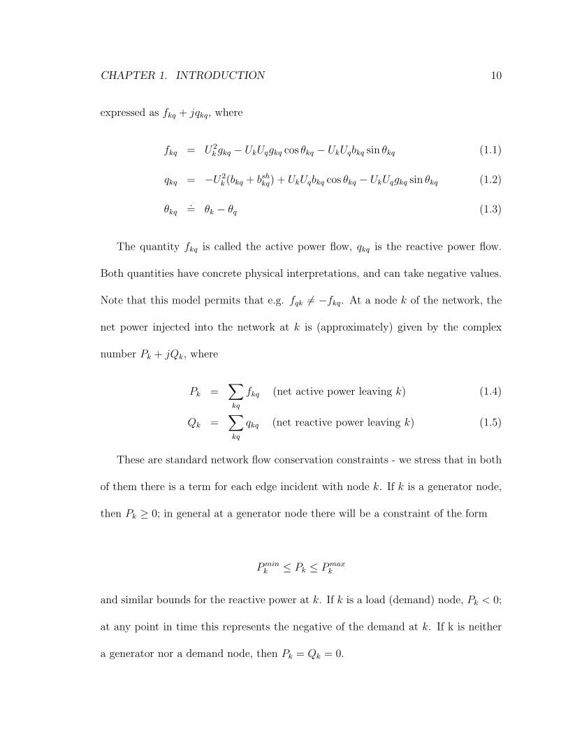
expressed as fkq + jqkq, where
fkq = U2kgkq − UkUqgkq cos θkq − UkUqbkq sin θkq (1.1)
qkq = −U2k (bkq + bshkq) + UkUqbkq cos θkq − UkUqgkq sin θkq (1.2)
θkq.= θk − θq (1.3)
The quantity fkq is called the active power flow, qkq is the reactive power flow.
Both quantities have concrete physical interpretations, and can take negative values.
Note that this model permits that e.g. fqk 6= −fkq. At a node k of the network, the
net power injected into the network at k is (approximately) given by the complex
number Pk + jQk, where
Pk =∑kq
fkq (net active power leaving k) (1.4)
Qk =∑kq
qkq (net reactive power leaving k) (1.5)
These are standard network flow conservation constraints - we stress that in both
of them there is a term for each edge incident with node k. If k is a generator node,
then Pk ≥ 0; in general at a generator node there will be a constraint of the form
Pmink ≤ Pk ≤ Pmax
k
and similar bounds for the reactive power at k. If k is a load (demand) node, Pk < 0;
at any point in time this represents the negative of the demand at k. If k is neither
a generator nor a demand node, then Pk = Qk = 0.

CHAPTER 1. INTRODUCTION 11
The model given by constraints (1.1)-(1.5) provides a fairly accurate approxima-
tion of the steady state behavior of a power grid. Nevertheless, it suffers from two
shortcomings: First, it can be expensive to solve, and second, the system may have
multiple solutions (the solution set may be discrete; less frequently, the system may
even be infeasible). Partly in order to remedy the second difficulty, the most popular
approaches to computing AC power flows rely on iterative methods, which require an
initial “guess” of the solution. Such a guess is relatively easy to arrive at when one
is familiar with the network being solved but not so if the network is in an unusual
configuration; an incorrect guess can lead to convergence to the “wrong” solution.
Human input in this loop is frequently used. Among the popular iterative meth-
ods used are Gauss-Seidel iterative method and the Newton-Raphson method. For a
detailed review of these methods we refer the interested reader to [3].
1.3.2 Linear Power Flow Models
In order to bypass the shortcomings of the AC power flow model, and primarily the
speed issue, a linear model is frequently used. This is the so-called DC flow model,
which relies on some estimations, primarily that θkq ≈ 0 for each edge {k, q} and
Uk ≈ 1 for any node k. The (approximate) active power constraint (1.1) becomes
− xkqfkq + θk − θq = 0 for all{k, q} (1.6)
where xkq.= − 1
bkqis the series resistance. This equation is analogous to Ohms law

CHAPTER 1. INTRODUCTION 12
applied to a resistor carrying a dc current:
• fkq is the dc current
• θk and θq are the dc voltages at resistor terminals
• xkq is the resistance for edge {k, q}.
Also note that because of (1.6), we have fqk = −fkq for each edge {k, q}, in other
words the two equations (1.6) corresponding to {k, q} are equivalent. Alternatively,
we can view the network as directed, and use a negative flow value to indicate flow
in the direction of the reversed edge.
When analyzing a power network, there is an additional, critical, operational re-
quirement. For each edge {k, q} there is a “capacity” ukq, representing a thermal limit.
In the DC ow model, we should have | fkq |≤ ukq. This (or the appropriate statement
in the AC flow model) is not a constraint that enters into the solution procedure - the
power flow values are determined by the physics of the network, whereas the capacity
constraint is simply a desirable outcome. Should an edge exceed its capacity, then
eventually it will burn up (how long this takes depends on the overload) but normally
protection equipment will disconnect the edge when the failure point is approached.
We stress that a small overload is tolerable and that the protection equipment will
not act immediately in such a case. Note: we will use the term “capacity” because
of its familiar interpretation in optimization.

CHAPTER 1. INTRODUCTION 13
From the description above, it is evident that the DC power flow model is a
rather parsimonious description of the underlying AC power flow model (1.1)-(1.5).
We would like to stress that the use of DC power flow model is very popular in
literature even when it is not clearly justified.
Finally we summarize the linearized, or DC power flow model, which we will use
for the most part in this thesis: We represent power grid by a directed network N ,
where:
• Each node corresponds to a “generator” (i.e., a supply node), or to a “load”
(i.e., a demand node), or to a node that neither generates nor consumes power.
• If node i corresponds to a generator, then there are values 0 ≤ Pmini ≤ Pmax
i .
If the generator is operated, then its output must be in the range [Pmini , Pmax
i ];
if the generator is not operated, then its output is zero. In general, we expect
Pmini > 0. We denote by C the set of generator nodes.
• If node i corresponds to a demand, then there is a value Dnomi (the “nominal”
demand value at node i). We will denote the set of demands by D.
• The arcs ofN represent power lines. For each arc (i, j), we are given a parameter
xij > 0 (the resistance) and a parameter uij (the capacity).
Given a set C of operating generators, a power flow is a solution to the system of
constraints given next. In this system, for each arc (i, j), we use a variable fij to

CHAPTER 1. INTRODUCTION 14
represent the (power) flow on (i, j) – possibly fij < 0, in which case power is effectively
flowing from j to i. In addition, for each node i we will have a variable θi (the “phase
angle” at i). Finally, if i is a generator node, then we will have a variable Pi, while if
i represents a demand node, we will have a variable Di. The constraints are:
∑(i,j)∈δ+(i)
fij −∑
(j,i)∈δ−(i)
fji =
Pi i ∈ C
−Di i ∈ D
0 otherwise
(1.7)
θi − θj − xijfij = 0 ∀(i, j) (1.8)
|fij| ≤ uij, ∀(i, j) (1.9)
Pmini ≤ Pi ≤ Pmax
i ∀i ∈ C (1.10)
0 ≤ Dj ≤ Dnomj ∀j ∈ D (1.11)
We will denote this system by P (N , C). Constraint (1.7) models flow conservation,
while (1.10) and (1.11) describe generator and demand node bounds. Optionally, one
may impose additional constraints, in particular bounds on the θi or on the quantities
|θi − θj| (over the arcs (i, j)).
Basic results
A useful property satisfied by the linearized model is given by the following result.
Lemma 1.3.1 Let C be given, and suppose N is connected. Then for any choice of

CHAPTER 1. INTRODUCTION 15
nonnegative values Pi (for i ∈ C) and Di (for i ∈ D) such that
∑i∈C
Pi =∑i∈D
Di, (1.12)
system (1.7)-(1.8) has a unique solution in the fij; thus, the solution is also unique
in the θi − θj (over the arcs (i, j)).
Proof. Let N denote the node-arc incidence of the network [1], let b be the vector
with an entry for each node, where bi = Pi for i ∈ C, bi = −Di for i ∈ D, and bi = 0
otherwise. Writing X for the diagonal matrix with entries xij, then (1.7)-(1.8) can
be summarized as
Nf = b, (1.13)
NT θ − Xf = 0. (1.14)
Pick an arbitrary node v; then system (1.13-1.14) has a solution iff it has one with θv =
0. As is well-known, N does not have full row rank, but writing N for the submatrix of
N with the row corresponding to v omitted then the connectivity assumption implies
that N does have full row rank [1]. In summary, writing b for the corresponding
subvector of b, we have that (1.13-1.14) has a solution iff
Nf = b, (1.15)
NTη − Xf = 0. (1.16)
where the vector η has an entry for every node other than v. Here, (1.16) implies
f = X−1NTη, and so (1.15) implies that η = (NX−1NT )−1b (where the matrix is

CHAPTER 1. INTRODUCTION 16
invertible since N has full row rank). Consequently, f = X−1NT (NX−1NT )−1b.
Remark 1.3.2 We stress that Lemma 1.3.1 concerns the subsystem of P (N , C)
consisting of (1.7) and (1.8). In particular, the “capacities” uij play no role in the
determination of solutions.
When the network is not connected Lemma 1.3.1 can be extended by requiring that
(1.12) hold for each component.
Definition 1.3.3 Let (f, θ, P,D) be feasible a solution to P (N , C). The throughput
of (f, θ, P,D) is defined as
∑i∈DDi∑
i∈DDnomi
. (1.17)
The throughput of N is the maximum throughput of any feasible solution to P (N , C).
1.4 Review of Basic Mathematics
In this section we present some background on some basic mathematical concepts
and notations that we have used throughout the thesis.
1.4.1 Network Flows
For general background on network flows we refer the reader to [1]. Matrix repre-
sentations of graphs have long been used to apply algebraic techniques to analyze

CHAPTER 1. INTRODUCTION 17
graphs. Here we review the node-arc incidence matrix and the Laplacian matrix, as
two of the commonly used representations for graphs. The node-arc incidence matrix
of a graph is used in flow problems, and we will use this representation to present
power flow equations. The Laplacian matrix for graphs, on the other hand, underlies
spectral graph theory, which can be used to analyze the connectedness of graphs.
Let G = (V,E) be a directed network defined by a set V of n nodes and a set E
of m directed arcs. We use (i, j) to denote an edge that goes from vertex i to vertex
j . We define the node-arc incidence matrix, N , of this graph as an n ×m matrix,
where the kth row of N represents the vertex k , and the lth column represents the
lth edge, (i, j) between nodes i and j. Each column has only two non-zeros at the
rows that represent the end vertices of the respective edge. The entry is −1 or 1,
depending on whether the respective edge is directed from or to the corresponding
vertex, respectively.
We will say that two nodes i and j are connected if the graph contains at least
one path from node i to node j. A graph is connected if every pair of its nodes is
connected; otherwise the graph is disconnected.
Next we turn our attention to defining Laplacians of graphs. The interested reader
is referred to [24] for more detailed material. We have a directed network G with n
nodes and m arcs and with node-arc incidence matrix N . We assume G is connected.

CHAPTER 1. INTRODUCTION 18
For a positive diagonal matrix Y ∈ Rm×m we will write
L = NYNT , J = L +1
n11T . (1.18)
where 1 ∈ Rn is the vector (1, 1, . . . , 1)T . L is called a generalized Laplacian. We have
that L is symmetric positive-semidefinite. If λ1 ≤ λ2 ≤ . . . ≤ λn are the eigenvalues
of L, and v1, v2, . . . , vn are the corresponding unit-norm eigenvectors, then
λ1 = 0, but λi > 0 for i > 1, (1.19)
because G is connected, and thus L has rank n− 1. The same argument shows that
since N1 = 0, we can assume v1 = n−1/2 1. Finally, since different eigenvectors are
are orthogonal, we have 1Tvi = 0 for 2 ≤ i ≤ n.
1.4.2 Benders’ Decomposition
The well known Benders’ decomposition technique [13] is based on the idea of exploit-
ing decomposable structure present in the formulation of a given problem so that its
solution can be obtained from the solution of several smaller sub-problems. One is
the follower problem which is obtained by fixing a number of decision variables of
the initial problem to a feasible value. The second problem is the restricted master
problem which is expected to provide the optimal solution after several iterations. At
each iteration a cut or (several) cuts are added to the master problem. The cuts are
deduced from the solution of the follower problem in each iteration of the algorithm.

CHAPTER 1. INTRODUCTION 19
In each iteration, cuts are appended to restricted master problem which is solved
again to optimality.
One can generally prove that Benders’ decomposition termites in a finite number
of iterations, though the number of iterations can be exponential. Benders’ decompo-
sition methods can be viewed as a special case of cutting-plane methods. As is the case
for cutting-plane methods for combinatorial optimization, there is no adequate gen-
eral theory to explain why Benders’ decomposition, when adequately implemented,
tends to converge in few iterations.
Benders’ decomposition algorithms have long enjoyed popularity in many con-
texts. In the case of stochastic programming with large number of scenarios, they
prove essential in that they effectively reduce a massively large continuous problem
into a number of much smaller independent problems. In the context of non-convex
optimization the appeal of decomposition is that it vastly reduces combinatorial com-
plexity.
1.4.3 Lagrangians
For a comprehensive discussion on Lagrangian duality see [2]. In mathematical pro-
gramming, the method of Lagrangian duality provides a construction for finding the
minimum of a function subject to constraints. The basic idea in Lagrangian duality
is to take the constraints into account by augmenting the objective function with a
weighted sum of the constraint functions.

CHAPTER 1. INTRODUCTION 20
One can use Lagrangian duality to derive the dual problem to any mathematical
program. The dual problem is always a convex optimization problem (i.e. minimizing
a convex function over a convex set) and thus is generally easier than the original
problem, both in terms of computational effort and optimality guarantees.
In the case of a convex optimization problem (subject to appropriate regular-
ity constraints) there is “strong duality”, i.e. the value of the original problem and
the value of the dual are the same. Strong duality does not, in general, hold for
non-convex optimization problems, in which case the dual merely provides a bound
(a lower bound in the case of a minimization problem). The non-zero gap between
the objective values of the original problem and its dual is known as the “duality gap”.

CHAPTER 2. THE “N - K” PROBLEM 21
Chapter 2
The “N - k” problem
In this chapter we present our algorithm for the N − k problem as applicable to the
linearized power flow model.
As discussed in the previous chapter, the linearized power flow model is an ap-
proximation to the AC power flow model which describes the steady state dynamics
of the power network. The issue of whether to use the more exact nonlinear formu-
lation, or the approximate DC formulation, is rather thorny. On the one hand, the
linearized formulation certainly is an approximation only. On the other hand, the
AC formulation can prove intractable or otherwise inappropriate (e.g. the formula-
tion may have multiple solutions), and, we stress, is itself in any case an approximate
model of the underlying physics.
For these reasons, studies that require multiple power flow computations tend to
rely on the linearized formulation. This will be the approach we take in this thesis,

CHAPTER 2. THE “N - K” PROBLEM 22
though some of our techniques extend directly to the AC model. An approach such as
ours can therefore be criticized because it relies on an ostensibly approximate model;
on the other hand we are able to focus more explicitly on the basic combinatorial
complexity that underlies the N − k problem. In contrast, an approach that uses the
AC model would have a better representation of the physics, but at the cost of not
being able to tackle the combinatorial complexity quite as effectively, for the simple
reason that the theory and computational machinery for linear programming are far
more mature, effective and scalable than those for nonlinear, nonconvex optimization.
In summary, both approaches present limitations and benefits. In this thesis, our bias
is toward explicitly handling the combinatorial nature of the problem.
A final point that we would like to stress is that whether we use the AC or DC
power flow model, the resulting problems have a far more complex structure than (say)
traditional single- or multi-commodity flow models because of side-constraints such
as (1.8). Constraints of this type give rise to counter-intuitive behavior reminiscent
of Braess’s Paradox [14].
The model we consider in this section can be further enriched by including many
other real-life constraints. For example, when considering the response to a contin-
gency one could insist that demand be curtailed in a (geographically) even-handed
pattern, and not in an aggregate fashion, as we do below and has been done in the
literature. Or we could impose upper bounds on the number of stand-by power units
that are turned on in the event of a contingency (and this itself could have a ge-

CHAPTER 2. THE “N - K” PROBLEM 23
ographical perspective). Many such realistic features suggest themselves and could
give rise to interesting extensions to the problem we consider here.
2.1 Problem Definition
We begin by formally defining the N − k problem : Let N be a network with n
nodes and m arcs representing a power grid. We denote the set of arcs by E and
the set of nodes by V . A fictional attacker wants to remove a small number of arcs
from N in order to maximize damage. Somewhat informally (and, as it turns out,
incompletely), the goal of the attacker is that in the resulting network all feasible
flows should have low throughput. At the same time, a controller is operating the
network; the controller responds to an attack by appropriately choosing the set C
of operating generators, their output levels, and the demands Di, so as to feasibly
obtain high throughput.
Thus, the attacker seeks to defeat all possible courses of action by the controller,
in other words, we are modeling the problem as a Stackelberg game between the
attacker and the controller, where the attacker moves first. To cast this in a precise
way we will use the following definition. We let 0 ≤ Tmin ≤ 1 be a given value.
Definition 2.1.1 Given a network N ,
• An attack A is a set of arcs removed by the attacker.

CHAPTER 2. THE “N - K” PROBLEM 24
• Given an attack A, the surviving network N − A is the subnetwork of N
consisting of the arcs not removed by the attacker.
• A configuration is a set C of generators.
• We say that an attack A defeats a configuration C, if either (a) the maximum
throughput of any feasible solution to P (N −A, C) is strictly less than Tmin,
or (b) no feasible solution to P (N −A, C) exists. Otherwise we say that C
defeats A.
• We say that an attack is successful, if it defeats every configuration.
• The min-cardinality attack problem consists in finding a successful attack
A with |A| minimum.
Our primary focus will be on the min-cardinality attack problem. Before proceeding
further we would like to comment on our model, specifically on the parameter Tmin.
In a practical use of the model, one would wish to experiment with different values
for Tmin – for the simple reason that an attack A which is not successful for a given
choice for Tmin could well be successful for a slightly larger value; e.g. no attack
or cardinality 3 or less exists that reduces demand by 31%, and yet there exists an
attack of cardinality 3 that reduces satisfied demand by 30%. In other words, the
minimum cardinality of a successful attack could vary substantially as a function of
Tmin.

CHAPTER 2. THE “N - K” PROBLEM 25
Given this fact, it might appear that a better approach to the power grid vul-
nerability problem would be to leave out the parameter Tmin entirely, and instead
redefine the problem to that of finding a set of k or fewer arcs to remove, so that the
resulting network has minimum throughput (here, k is given). We will refer to this
as the budget-k min-throughput problem. However, there are reasons why this latter
problem is less attractive than the min-cardinality problem.
(a) Clearly, in a sense, the min-cardinality and min-throughput problems are duals
of each other. A modeler considering the min-throughput problem would want
to run that model multiple times, because given k, the value of the budget-k
min-throughput problem could be much smaller than the value of the budget-
(k+1) min-throughput problem. For example, it could be the case that using a
budget of k = 2, the attacker can reduce throughput by no more than 5%; but
nevertheless with a budget of k = 3, throughput can be reduced by e.g. 50%.
In other words, even if a network is “resilient” against attacks of size ≤ 2, it
might nevertheless prove very vulnerable to attacks of size 3. For this reason,
and given that the models of grids, power flows, etc., are rather approximate,
a practitioner would want to test various values of k – this issue is obviously
related to what percentage of demand loss would be considered tolerable, in
other words, the parameter Tmin.
(b) From an operational perspective it should be straightforward to identify rea-

CHAPTER 2. THE “N - K” PROBLEM 26
sonable values for the quantity Tmin; whereas the value k is more obscure and
bound to models of how much power the adversary can wield.
(c) Because of a subtlety that arises from having positive quantities Pmini , explained
next, it turns out that the min-throughput problem is significantly more com-
plex and is difficult to even formulate in a compact manner.
We will now expand on (c). One would expect that when a configuration C is defeated
by an attack A, it is because only small throughput solutions are feasible in N −A.
However, because the lower bounds Pmini are in general strictly possible, it may also
be the case that no feasible solution to P (N −A, C) exists.
Example 2.1.2 Consider the following example on a network N with three nodes
(see Figure 2.1), where
1. Nodes 1 and 2 represent generators; Pmin1 = 2, Pmax
1 = 4, Pmin2 = 0, and
Pmax2 = 4,
2. Node 3 is a demand node with Dnom3 = 6. Furthermore, Tmin = 1/2.
3. There are three arcs; arc (1, 2) with x12 = 1 and u12 = 1, arc (2, 3) with x23 = 1
and u23 = 5, and arc (1, 3) with x13 = 1 and u13 = 3.
When the network is not attacked, the following solution is feasible: P1 = P2 = 3,
D3 = 6, f12 = 0, f13 = f23 = 3, θ1 = θ2 = 0, θ3 = −3. This solution has throughput

CHAPTER 2. THE “N - K” PROBLEM 27
1
2 3
D3_nom = 6P2_min = 0, P4_max = 4
x_23 = 1, u_23 = 5
x_13 = 1x_12 = 1, u_12 = 1
P1_min = 2, P1_max = 4
u_13 = 3
Figure 2.1: A simple example.
100%. On the other hand, consider the attack A consisting of the single arc (1, 3),
and suppose we choose the configuration C = {1, 2} (i.e. we operate both generators).
Since Pmin1 > u12, P (N −A, C) has no feasible solution, and A defeats C (in spite
of the fact that we can still meet 100% of the demand).
Likewise, A defeats the configuration where we only operate generator 1. Thus,
A is successful if and only if it also defeats the configuration where we only operate
generator 2, which it does not since in that configuration we can feasibly send up to
four units of flow on (2, 3) and Tmin = 1/2 < 4/6.
As the example highlights, it is important to understand how an attack A can
defeat a particular configuration C. It turns out that there are three different ways
for this to happen.

CHAPTER 2. THE “N - K” PROBLEM 28
(i) Consider a partition of the nodes of N into two classes, N1 and N2. Write
Dk =∑
i∈D∩Nk
Dnomi , k = 1, 2, and (2.1)
P k =∑
i∈C∩Nk
Pmaxi , k = 1, 2, (2.2)
e.g. the total (nominal) demand in N1 and N2, and the maximum power gener-
ation in N1 and N2, respectively. The following condition, should it hold, would
guarantee that A defeats C:
Tmin∑j∈D
Dnomj −min{D1, P 1} −min{D2, P 2} >
∑(i,j)/∈A : i∈N1, j∈N2
uij +
∑(i,j)/∈A : i∈N2, j∈Nj
uij.(2.3)
To understand this condition, note that for k = 1, 2, min{Dk, P k} is the maxi-
mum demand within Nk that could possibly be met using power flows that do
not leave Nk. Consequently the left-hand side of (2.3) is a lower bound on the
amount of flow that must travel between N1 and N2, whereas the right-hand
side of (2.3) is the total capacity of arcs between N1 and N2 under attack A.
In other words, condition (2.3) amounts to a mismatch between demand and
supply. A special case of (2.3) is that where in N −A there are no arcs between
N1 and N2, i.e. the right-hand side of (2.3) is zero.
(ii) Consider a partition of the nodes of N into two classes, N1 and N2, such that
in N −A there are no arcs between N1 and N2. Then attack A defeats C if
∑iD∩∈N1
Dnomi <
∑i∈C∩N1
Pmini , (2.4)

CHAPTER 2. THE “N - K” PROBLEM 29
i.e., the minimum power output withinN1 exceeds the maximum demand within
N1. Note that (ii) may apply even if (i) does not.
(iii) Even if (i) and (ii) do not hold, it may still be the case that the system (1.7)-
(1.11) does not admit a feasible solution. To put it differently, suppose that
for every choice of demand values 0 ≤ Di ≤ Dnomi (for i ∈ D) and supply
values Pmini ≤ Pi ≤ Pmax
i (for i ∈ C) such that∑
i∈C Pi =∑
i∈DDi the unique
solution to system (1.7)-(1.8) in network N −A (as per Lemma 1.3.1) does not
satisfy the “capacity” inequalities |fij| ≤ uij for all arcs (i, j) ∈ N − A. Then
A defeats C. This is the most subtle case of all – it involves the interplay of
flow conservation and Ohm’s law.
Note that in particular in case (ii), the defeat condition is unrelated to throughput.
Nevertheless, should case (ii) arise, it is clear that the attack has succeeded (against
configuration C) – this makes the min-throughput problem difficult to model; our
formulation for the min-cardinality problem, given in Section 2.2, does capture the
three defeat criteria above.
From a practical perspective, it is important to handle models where the values
Pmini are positive. It is also important to model standby generators that are turned
on when needed, and to model the turning off of generators that are unable to dis-
pose of their minimum power output, post-attack. All these features arise in practice.

CHAPTER 2. THE “N - K” PROBLEM 30
Example 2.1.2 above shows that models where generators cannot be turned off can
exhibit unreasonable behavior. Of course, the ability to select the operating genera-
tors comes at a cost, in that in order to certify that an attack is successful we need
to evaluate, at least implicitly, a possibly exponential number of control possibilities.
As far as we can tell, most (or all) prior work in the literature does require that
the controller must always use the configuration G consisting of all generators. As the
example shows, however, if the quantities Pmini are positive there may be attacks A
such that P (N −A, G) is infeasible. Because of this fact, algorithms that rely on
direct application of Benders’ decomposition or bilevel programming are problematic,
and invalid formulations can be found in the literature.
Our approach works with general Pmin ≥ 0 quantities; thus, it also applies to the
case where we always have Pmini = 0. In this case our formulation is simple enough
that a commercial integer program solver can directly handle instances larger than
previously reported in the literature.
2.1.1 Non-monotonicity
Consider the example in Figure 2.2, where we assume Tmin = 0.3. Notice that there
are two parallel copies of arcs (2, 4) and (3, 5), each with capacity 10 and impedance 1.
It is easy to see that the network with no attack is feasible: we operate generator 1 and
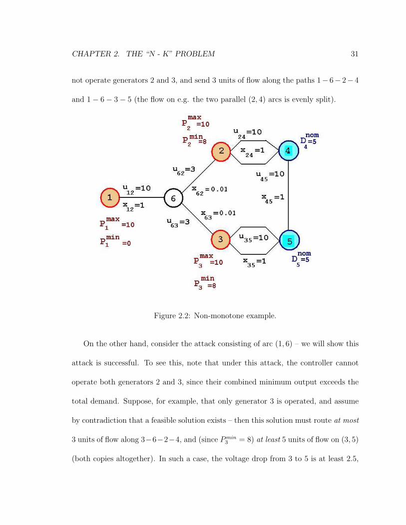
CHAPTER 2. THE “N - K” PROBLEM 31
not operate generators 2 and 3, and send 3 units of flow along the paths 1− 6− 2− 4
and 1− 6− 3− 5 (the flow on e.g. the two parallel (2, 4) arcs is evenly split).
Figure 2.2: Non-monotone example.
On the other hand, consider the attack consisting of arc (1, 6) – we will show this
attack is successful. To see this, note that under this attack, the controller cannot
operate both generators 2 and 3, since their combined minimum output exceeds the
total demand. Suppose, for example, that only generator 3 is operated, and assume
by contradiction that a feasible solution exists – then this solution must route at most
3 units of flow along 3−6−2−4, and (since Pmin3 = 8) at least 5 units of flow on (3, 5)
(both copies altogether). In such a case, the voltage drop from 3 to 5 is at least 2.5,

CHAPTER 2. THE “N - K” PROBLEM 32
whereas the voltage drop from 3 to 4 is at most 1.56. In other words, θ4 − θ5 ≥ 0.94,
and so we will have f45 ≥ 0.94 – thus, the net inflow at node 5 is at least 5.94. Hence
the attack is indeed successful.
However, there is no successful attack consisting of arc (1, 6) and another arc. To
see this, note that if one of (2, 6), (3, 6) or (4, 5) are also removed then the controller
can just operate one of the two generators 2, 3 and meet eight units of demand.
Suppose that (say) one of the two copies of (3, 5) is removed (again, in addition to
(1, 6)). Then the controller operates generator 2, sending 2.5 units of flow on each of
the two parallel (2, 4) arcs; thus θ2 − θ4 = 2.5. The controller also routes 3 units of
flow along 2 − 6 − 3 − 5, and therefore θ2 − θ5 = 3.06. Consequently θ4 − θ5 = .56,
and f45 = .56, resulting in a feasible flow which satisfies 4.44 units of demand at 4
and 3.56 units of demand at 5.
In fact, it is straightforward to show that no successful attack of of cardinality 2
exists – hence we observe non-monotonicity.
By elaborating on the above, one can create examples with arbitrary patterns in
the cardinality of successful attacks. One can also generate examples that exhibit
non-monotone behavior in response to controller actions. In both cases, the non-
monotonicity can be viewed as a manifestation of the so-called “Braess’s Paradox”
[14]. In the above example we can observe combinatorial subtleties that arise from
the ability of the controller to choose which generators to operate, and from the lower
bounds on output in operating generators. Nevertheless, it is clear that the critical

CHAPTER 2. THE “N - K” PROBLEM 33
core reason for the complexity is the interaction between voltages and flows, i.e. be-
tween “Ohm’s law” (1.8) and flow conservation (1.7) – the combinatorial attributes of
the problem exercise this interaction. Thus, we view it as crucial that an optimization
model address the interaction in an explicit manner.
2.1.2 Brief review of previous work
The min-cardinality problem, as defined above, can be viewed as a bilevel program
(see 1.1 for definition of bilevel programming) where both the master problem and
the subproblem are mixed-integer programs – the master problem corresponds to
the attacker (who chooses the arcs to remove) and the subproblem to the controller
(who chooses the generators to operate). In general, such problems are extremely
challenging. A recent general-purpose algorithm for such integer programs is given in
[21].
Alternatively, each configuration of generators can be viewed as a “scenario”. In
this sense our problem resembles a stochastic program, although without a probabil-
ity distribution. Recent work [22] considers a single commodity max-flow problem
under attack by an interdictor with a limited attack budget; where an attacked arc is
removed probabilistically, leading to a stochastic program (to minimize the expected
max flow). A deterministic, multi-commodity version of the same problem is given
in [23].
Previous work on the power grid vulnerability models has focused on cases where

CHAPTER 2. THE “N - K” PROBLEM 34
either the generator lower bounds Pmini are all zero, or all generators must be operated
(the single configuration case). Algorithms for these problems have either relied
on heuristics, or on mixed-integer programming techniques, usually a direct use of
Benders’ decomposition or bilevel programming. [5] considers a version of the min-
throughput problem with Pmini = 0 for all generators i, and presents an algorithm
using Benders’ decomposition (also see references therein). They analyze the so-called
IEEE One-Area and IEEE Two-Area test cases, with, respectively, 24 nodes and 38
arcs, and 48 nodes and 79 arcs. Also see [4].
[6] studies the IEEE One-Area test case, and allows Pmini > 0, but does not allow
generators to be turned off; the authors present a bilevel programming formulation
which, unfortunately, is incorrect, due to reasons outlined above.
2.2 An algorithm for the min-cardinality problem
In this section we will describe an iterative algorithm for the min-cardinality attack
problem. The algorithm iterates in Benders-like fashion, solving at each iteration two
mixed-integer programs. Before describing the algorithm we need to introduce some
notation and concepts.
Let A be a given attack. Suppose the controller attempts to defeat the attacker by
choosing a certain configuration C of generators. Denote by zA the indicator vector
for A, i.e. zAij = 1 iff (i, j) ∈ A. Then the controller needs to solve the following linear

CHAPTER 2. THE “N - K” PROBLEM 35
program:
KC(A) : tC(zA)
.= min t (2.5)
Subject to:
∑(i,j)∈δ+(i)
fij −∑
(j,i)∈δ−(i)
fji =
Pi i ∈ G
−Di i ∈ D
0 otherwise
(2.6)
θi − θj − xijfij = 0 ∀ (i, j) /∈ A (2.7)
uij t − |fij| ≥ 0, ∀ (i, j) /∈ A (2.8)
fij = 0, ∀(i, j) ∈ A (2.9)
Pmini ≤ Pi ≤ Pmax
i ∀i ∈ C (2.10)
Pi = 0, ∀i ∈ G − C (2.11)∑j∈D
Dj ≥ Tmin
(∑j∈D
Dnomj
), (2.12)
0 ≤ Dj ≤ Dnomj ∀j ∈ D (2.13)
Remark 2.2.1 Using the convention that the value of an infeasible linear program
is infinite, A defeats C if and only if tC(zA) > 1.
Thus, an attackA is not successful if and only if we can find C ⊆ G with tC(zA) ≤ 1;
we test for this conditions by solving the problem:
minC⊆G
tC(zA).

CHAPTER 2. THE “N - K” PROBLEM 36
This is done by replacing, in the above formulation, equations (2.10), (2.11) with
Pmini yi ≤ Pi ≤ Pmax
i yi, ∀i ∈ G, (2.14)
yi = 0 or 1, ∀i ∈ G. (2.15)
Here, yi = 1 if the controller operates generator i.
The min-cardinality attack problem can now be written as follows:
min∑(i,j)
zij (2.16)
tC (z) > 1, ∀ C ⊆ G, (2.17)
zij = 0 or 1, ∀ (i, j). (2.18)
This formulation, of course, is impractical, because we do not have a compact way
of representing any of the constraints (2.17), and there are an exponential number of
them.
Putting these issues aside, we can outline an algorithm for the min-cardinality
attack problem. Our algorithm will be iterative, and will maintain a “master attacker”
mixed-integer program which will be a relaxation of (2.16)-(2.18) – i.e. it will have
objective (2.16) but weaker constraints than (2.17). Initially, the master attacker
MIP will include no variables other than the z variables, and no constraints other
than (2.18). The algorithm proceeds as follows.

CHAPTER 2. THE “N - K” PROBLEM 37
Basic algorithm for min-cardinality attack problem
Iterate:
1. Attacker: Solve master attacker MIP and let z∗ be its
solution.
2. Controller: Search for a set C of generators such that tC(z∗) ≤ 1.
(2.a) If no such set C exists, EXIT:∑ij z∗ij is the minimum cardinality of a successful attack.
(2.b) Otherwise, suppose such a set C is found.
Add to the master attacker MIP a system of valid inequalities
that cuts off z∗.
Go to 1.
As discussed above, the search in Step 2 can be implemented by solving a mixed
integer program. Since in 2.b we add valid inequalities to the master, then inductively
we always have a relaxation of (2.16)-(2.18) and thus the value of the master at any
execution of step 1, i.e. the value∑
ij z∗ij, is a lower bound on the cardinality of any
successful attack. Thus the exit condition in step 2.a is correct, since it proves that
the attack implied by z∗ is successful.
The implementation of Case 2.b, on the other hand, requires some care. Assuming
we are in case 2.b, we have that tC(z∗) ≤ 1, and certainly the linear program KC(A)
is feasible. The optimal dual solution would therefore (apparently) furnish a Benders
cut that cuts off z∗. However this would be incorrect since the structure of constraints

CHAPTER 2. THE “N - K” PROBLEM 38
(2.5)-(2.13)) depends on z∗ itself.
Instead, we need to proceed as in two-stage stochastic programming with recourse,
where the z variables play the role as “first-stage” variables and also appear in the
second-stage problem (the subproblem); solutions to the dual of the second-stage
problem can then be used to generate cuts to add to the master problem. Toward
this goal, we proceed as follows, given C and z∗:
B.1 Write the dual of KC(∅).
B.2 As is standard in interdiction-type problems (see [23], [22], [21], [5]), the dual is
then “combinatorialized” by adding the z variables and additional constraints.
For example, if βij indicates the dual of constraint (2.7), then we add, to the
dual of KC(∅), inequalities of the form
βij −M1ijzij ≤ 0, −βij −M1
ijzij ≤ 0,
for an appropriate constant M1ij > 0. We proceed similarly with constraint (2.8),
obtaining the “combinatorial dual”. This combinatorial dual is the functional
equivalent of the second-stage problem in stochastic programming.
B.3 Fix the zij variables in the combinatorial dual to z∗; this yields a problem that
is equivalent to KC(z∗) and has the general structure
tC(z∗) = max cTv
Pv ≤ b + Qz∗. (2.19)

CHAPTER 2. THE “N - K” PROBLEM 39
Here, the v are variables, P and Q are matrices, and b is a vector, of appro-
priate dimensions; and we have a maximization problem since the KC() are
minimization problems. We obtain a cut of the form
αT (b+Qz) ≥ 1 + ε
where ε > 0 is a small constant and α is the vector of optimal dual variables to
(2.19). Since by assumption tC(z∗) ≤ 1 this inequality cuts off z∗.
Note the use of the tolerance ε. The use of this parameter gives more power to the
controller, i.e. “borderline” attacks are not considered successful. In a strict sense,
therefore, we are not solving the optimization problem to exact precision; nevertheless
in practice we expect our relaxation to have negligible impact so long as ε is small.
A deeper issue here is how to interpret truly borderline attacks that are successful
according to our strict model (and which our use of ε disallows); we expect that
in practice such attacks would be ambiguous and that the approximations incurred
in modeling power flows, estimating demands levels, and so on, not to mention the
numerical sensitivity of the integer and linear solvers being used, would have a far
more significant impact on precision.
2.2.1 Discussion
In order to make the outline provided in B.1-B.3 into a formal algorithm, we need
to specify the constants M1ij. As is well-known, the folklore of integer programming

CHAPTER 2. THE “N - K” PROBLEM 40
dictates that the M1ij should be chosen small to improve the quality of the linear
programming relaxation of the master problem.
While this is certainly true, we have found that popular optimization packages
show significant numerical instability when solving power flow linear programs. In
fact, in our experience it is primarily this behavior that mandates that the M1ij should
be kept as small as possible. In particular we do not want the M1ij to grow with net-
work since this would lead to an nonscalable approach.
It turns out that our formulation KC(A) is not ideal toward this goal. A partic-
ularly thorny issue is that the attack A may disconnect the network, and proving
“reasonable” upper bounds on the dual variables to (for example) constraint (2.6),
when the network is disconnected, does not seem possible. In the next section we
describe a different formulation for the min-cardinality attack problem which is much
better in this regard. Our eventual algorithm will apply steps B.1 - B.3 to this im-
proved formulation, while the rest of our basic algorithmic methodology as described
above will remain unchanged.

CHAPTER 2. THE “N - K” PROBLEM 41
2.3 A better mixed-integer programming formula-
tion
As before, let A be an attack and C a (given) configuration of generators. Let yC ∈ RG
be the indicator vector for C, i.e. yCi = 1 if i ∈ C and yCi = 0 otherwise. Consider the
following linear program:
K∗C(A) : t∗C(zA)
.= min t (2.20)
Subject to:
(αCi )∑
(i,j)∈δ+(i)
fij −∑
(j,i)∈δ−(i)
fji =
Pi i ∈ G
−Di i ∈ D
0 otherwise
(2.21)
(βCij) θi − θj − xijfij = 0 ∀ (i, j) /∈ A (2.22)
(pCij, qCij) uij t − |fij| ≥ 0, ∀ (i, j) /∈ A (2.23)
(ωC+ij , ωC−ij ) t − |fij| ≥ 1, ∀ (i, j) ∈ A (2.24)
(γC+i , γC+i ) Pmini yCi ≤ Pi ≤ Pmax
i yCi ∀i ∈ G (2.25)
(µC)∑j∈D
Dj ≥ Tmin
(∑j∈D
Dnomj
), (2.26)
(∆Cj ) Dj ≤ Dnomj ∀j ∈ D (2.27)
P ≥ 0, D ≥ 0. (2.28)
To the left of each constraint we have indicated the corresponding dual variable –

CHAPTER 2. THE “N - K” PROBLEM 42
(2.23) is really two constraints written as one, and the same with (2.24).
Note that we do not force fij = 0 for (i, j) ∈ A. Moreover arcs (i, j) ∈ A are also
exempted from constraint (2.22). Thus, the controller has significantly more power
than in KC(A). However, because of constraint (2.24), we have t∗C(zA) > 1 as soon
as any of the arcs in A actually carries flow. We can summarize these remarks as
follows:
Remark 2.3.1 A defeats C if and only if t∗C(zA) > 1.
Note that the above formulation depends on C only through constraint (2.25). Us-
ing appropriate matrices Af , Aθ, AP , AD, At, and vector b, the formulation can be
abbreviated as
K∗C(A) : t∗C(zA)
.= min t
Subject to:
Aff + Aθθ + APP + ADD + Att ≥ b
Pmini yCi ≤ Pi ≤ Pmax
i yCi , ∀i ∈ G

CHAPTER 2. THE “N - K” PROBLEM 43
Allowing the y quantities to become 0/1 variables, we obtain the problem
t∗(zA).= min t (2.29)
Subject to:
Aff + Aθθ + APP + ADD + Att ≥ b (2.30)
Pmini yi ≤ Pi ≤ Pmax
i yi, ∀i ∈ G (2.31)
yi = 0 or 1, ∀i ∈ G. (2.32)
This is the controller’s problem: we have that t∗(zA) ≤ 1 if and only if there exists
some configuration of the generators that defeats A.
However, for the purposes of this section, we will assume C is given and that the yC
are constants. We can now write the dual of K∗C(A), suppressing the index C from
the variables, for clarity.
AC(A) : max∑i∈G
yCi Pmini γ−i −
∑i∈G
yCi Pmaxi γ+
i −∑j∈D
Dnomj ∆j +
∑j∈D
Dnomj µj +
∑(i,j)∈E
(ω+ij + ω−ij)
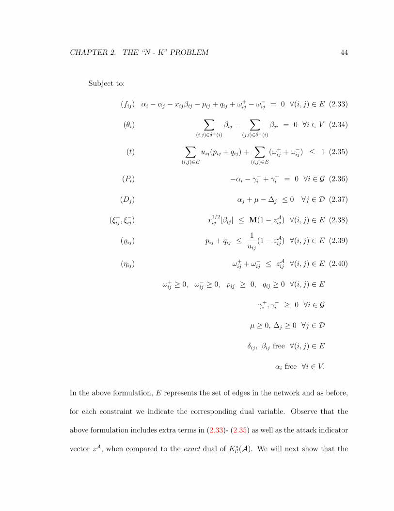
CHAPTER 2. THE “N - K” PROBLEM 44
Subject to:
(fij) αi − αj − xijβij − pij + qij + ω+ij − ω−ij = 0 ∀(i, j) ∈ E (2.33)
(θi)∑
(i,j)∈δ+(i)
βij −∑
(j,i)∈δ−(i)
βji = 0 ∀i ∈ V (2.34)
(t)∑
(i,j)∈E
uij(pij + qij) +∑
(i,j)∈E
(ω+ij + ω−ij) ≤ 1 (2.35)
(Pi) −αi − γ−i + γ+i = 0 ∀i ∈ G (2.36)
(Dj) αj + µ−∆j ≤ 0 ∀j ∈ D (2.37)
(ξ+ij , ξ
−ij) x
1/2ij |βij| ≤ M(1− zAij ) ∀(i, j) ∈ E (2.38)
(%ij) pij + qij ≤1
uij(1− zAij ) ∀(i, j) ∈ E (2.39)
(ηij) ω+ij + ω−ij ≤ zAij ∀(i, j) ∈ E (2.40)
ω+ij ≥ 0, ω−ij ≥ 0, pij ≥ 0, qij ≥ 0 ∀(i, j) ∈ E
γ+i , γ
−i ≥ 0 ∀i ∈ G
µ ≥ 0, ∆j ≥ 0 ∀j ∈ D
δij, βij free ∀(i, j) ∈ E
αi free ∀i ∈ V.
In the above formulation, E represents the set of edges in the network and as before,
for each constraint we indicate the corresponding dual variable. Observe that the
above formulation includes extra terms in (2.33)- (2.35) as well as the attack indicator
vector zA, when compared to the exact dual of K∗C(A). We will next show that the

CHAPTER 2. THE “N - K” PROBLEM 45
above formulation is equivalent to the exact dual of K∗C(A).
The dual constraint for variable fij in K∗C(A) is given by :
αi − αj − xijβij − pij + qij = 0 ∀(i, j) s.t. zAij = 0
αi − αj + ω+ij − ω−ij = 0 ∀(i, j) s.t. zAij = 1
Constraints (2.38) and (2.39) force βij = pij = qij = 0 when zAij = 1 while (2.40)
insures ω+ij = ω−ij = 0 when zAij = 0. Hence, the above two dual constraints can be
combined together and expressed as (2.33). The extra terms in (2.34) and (2.35) can
be explained similarly. Hence the above formulation AC(A) is equivalent to the dual
of K∗C(A).
In (2.38), M is an appropriately chosen constant (we will provide a precise value
for it below). Note that we are scaling βij by x1/2ij – this is allowable since x
1/2ij > 0;
the reason for this scaling will become clear below.
Abbreviating
(αC, βC, pC, qC, ωC+, ωC−, γC−, γC+, µC,∆C) = ψC,
we have that AC(A) can be rewritten as:
max{wTC ψ
C : AψC ≤ b + B(1− zA
) }(2.41)
where A, B, wC and b are appropriate matrices and vectors. Consequently, we can

CHAPTER 2. THE “N - K” PROBLEM 46
now rewrite the min-cardinality attack problem:
min∑(i,j)
zij (2.42)
Subject to: tC ≥ 1 + ε, ∀ C ⊆ G (2.43)
wTC ψC − tC ≥ 0, ∀ C ⊆ G, (2.44)
AψC + Bz ≤ b + B ∀ C ⊆ G, (2.45)
zij = 0 or 1, ∀ (i, j). (2.46)
This formulation, of course, is exponentially large. An alternative is to use Ben-
ders cuts – having solved the linear program AC(A), let (f , θ, t, P , D, ξ+, ξ−, %, η) be
optimal dual variables. Then the resulting Benders cut is
tC +∑
(i,j)∈E
((ξ+ij + ξ−ij)M(1− zij)) +
∑(i,j)∈E
(1
uij%ij(1− zij)) +
∑(i,j)∈E
ηijzij ≥ 1 + ε,
(2.47)
We can now update our algorithmic template for the min-cardinality problem.

CHAPTER 2. THE “N - K” PROBLEM 47
Updated algorithm for min-cardinality attack problem
Iterate:
1. Attacker: Solve master attacker MIP, obtaining attack A.
2. Controller: Solve the controller’s problem (2.29)-(2.32) to search
for a set C of generators such that t∗C(zA) ≤ 1.
(2.a) If no such set C exists, EXIT:
A is a minimum cardinality successful attack.
(2.b) Otherwise, suppose such a set C is found. Then
(2.b.1) Add to the master the Benders’ cut (2.47), and, optionally
(2.b.2) Add to the master the entire system (2.43)-(2.45),
Go to 1.
Clearly, option (2.b.2) can only be exercised sparingly (if ever). Below we will discuss
how we choose, in our implementation, between (2.b.1) and (2.b.2). We will also
describe how to (significantly) strengthen the straightforward Benders cut (2.47).
One point to note is that the cuts (or systems) arising from different configurations
C reinforce one another.
At each iteration of the algorithm, the master attacker MIP becomes a stronger
relaxation for the min-cardinality problem, and thus its solution in step 1 provides a
lower bound for the problem. Thus, if in a certain execution of step 2 we certify that
t∗C(zA) > 1 for every configuration C, we have solved the min-cardinality problem to
optimality.

CHAPTER 2. THE “N - K” PROBLEM 48
What we have above is a complete outline of our algorithm. In order to make the
algorithm effective we need to further sharpen the approach. In particular, we need
set the constant M to as small a value as possible, and we need to develop stronger
inequalities than the basic Benders’ cuts.
2.3.1 Setting M
In this section we show how to choose for M a value that does not grow with network
size (see Section 2.2.1 for detailed discussion).
Lemma 2.3.2 We can set
M = max(i,j)∈E
{1
√xij uij
.
}(2.48)
Proof. Given an attack A, consider a connected component K of N −A. For any arc
(i, j) with both ends in K, ω+ij + ω−ij = 0 by (2.40). Hence we can rewrite constraints
(2.33)-(2.34) over all arcs with both ends in K as follows:
NTKαK − XKβK = pK − qK , (2.49)
NKβK = 0. (2.50)
Here, NK is the node arc incidence matrix of K, αK , βK , pK , qK are the restrictions
of α, β, p, q to K, and XK is the diagonal matrix diag{xij : (i, j) ∈ K}. From this
system we obtain
NKX−1K NKαK = NKX
−1K (pK − qK). (2.51)

CHAPTER 2. THE “N - K” PROBLEM 49
The matrix NKX−1K NK has one-dimensional null space and thus we have one degree of
freedom in choosing αK . Thus, to solve (2.51), we can remove from NK an arbitrary
row, obtaining NK , and remove the same row from αK , obtaining αK . Thus, (2.51)
is equivalent to:
NKX−1K NKαK = NKX
−1K (pK − qK), (2.52)
The matrix NKX−1K NK and thus (2.52) has a unique solution (given pK − qK); we
complete this to a solution to (2.51) by setting to zero the entry of αK that was
removed. Moreover,
X−1/2K NT
KαK = X−1/2K NT
KαK = X−1/2K NT
K(NKX−1K NT
K)−1NKX−1K (pK − qK). (2.53)
The matrix
M = X−1/2K NT
K (NKX−1K NT
K)−1 NKX−1/2K
is symmetric and idempotent, e.g. MMT = I. Thus, from (2.53) we get
‖X−1/2K NT
KαK‖2 ≤ ‖M‖2 ‖X−1/2K (pK − qK)‖2 ≤ ‖X−1/2
K (pK − qK)‖2, (2.54)
where the last inequality follows from the idempotent attribute. Because of con-
straints (2.35), (2.39) and (2.40), we can see that the right-hand side of (2.54) is
upper-bounded by the value of the convex maximization problem,
max∑
(i,j)∈E
x−1ij (pij − qij)2 (2.55)
s.t.∑
(i,j)∈E
uij(pij + qij) ≤ 1 (2.56)
pij ≥ 0, qij ≥ 0, (2.57)

CHAPTER 2. THE “N - K” PROBLEM 50
which, as is easily seen, equals
max(i,j)∈E
{1
xiju2ij
}.
2.3.2 Tightening the formulation
In this Section we describe a family of inequalities that are valid for the attacker
problem. These cuts seek to capture the interplay between the flow conservation
equations and Ohm’s law. First we present a technical result.
Lemma 2.3.3 Let Q be matrix with r rows with rank r, and let A = QT (QQT )−1Q ∈
Rr×r. Let B := I − A. Then for any p ∈ Rr we have
‖p‖22 = ‖Ap‖2
2 + ‖Bp‖22 (2.58)
‖p‖1 ≥ |(Ap)j|+ |(Bp)j| ∀j = 1 . . . r (2.59)
Proof. A and B are symmetric and idempotent, i.e., A2 = A, B2 = B, and any
p ∈ Rr can be written as p = Ap+Bp. Multiplying equation this by p and using the
fact that A and B are symmetric and idempotent we get (2.58):
pTp = pTAp+ pTBp (2.60)
= pTA2p+ pTB2p (2.61)
‖p‖22 = ‖Ap‖2
2 + ‖Bp‖22 (2.62)
We also have ATB = A(I − A) = A − A2 = 0, so yTATBy = 0 for any y ∈ Rr.
Thus, if we rename Ap = x and Bp = y, then the following holds: p = x+ y, xTy =

CHAPTER 2. THE “N - K” PROBLEM 51
0, ‖p‖22 = ‖x‖2
2 + ‖y‖22.
Let 1 ≤ j ≤ r. We have
‖p‖22 − (|xj|+ |yj|)2 = ‖x‖2
2 + ‖y‖22 − (|xj|+ |yj|)2 =
∑i,i 6=j
x2i +
∑i,i 6=j
y2i − 2|xjyj|
where the first equality follows from (2.58). Since xTy = 0, we have |xjyj| =
|∑
i,i 6=j xiyi|. Hence,
∑i,i 6=j
x2i +
∑i,i 6=j
y2i − 2|xjyj| =
∑i,i 6=j
x2i +
∑i,i 6=j
y2i − 2
∣∣∣∣∣∑i,i 6=j
xiyi
∣∣∣∣∣ (2.63)
≥∑i,i 6=j
x2i +
∑i,i 6=j
y2i − 2
∑i,i 6=j
|xiyi| (2.64)
=∑i,i 6=j
(|xi| − |yi|)2 (2.65)
≥ 0 (2.66)
So we have ‖p‖22 − (|xj|+ |yj|)2 ≥ 0, which implies ‖p‖1 ≥ ‖p‖2 ≥ (|xj|+ |yj|) ∀j =
1 . . . r.
As a consequence of this result we now have:
Lemma 2.3.4 Given configuration C, the following inequalities are valid for system
(2.45)-(2.46) for each (i, j) ∈ E:
x− 1
2ij |αCi − αCj |+ x
12ij|βCij| ≤ x
− 12
ij wCij + M(1− zij) (2.67)
x− 1
2ij |αCi − αCj |+ x
12ij|βCij| ≤
∑(k,l)
x− 1
2kl (pCkl + qCkl) + wCij (2.68)
where M := max(k,l)∈E{ 1√xklukl
} as before.

CHAPTER 2. THE “N - K” PROBLEM 52
Proof. Suppose first that zij = 0. Let K be the component containing (i, j) after the
attack. Then by (2.53) and (2.49),
X−1/2NTKαC = AX−1/2(pC − qC), (2.69)
X1/2βC = (I − A)X−1/2(pC − qC), (2.70)
where A = X−1/2NKT
(NKX−1NK
T)−1NKX
−1/2. Thus, we have
x−1/2ij |αCi − αCj |+ x
1/2ij |βCij| ≤
∑(k,l)
x−1/2kl (pCkl + qCkl) ≤ M (2.71)
where the first inequality follows from (2.59) proved in Lemma 2.3.3, and the second
bound is obtained as in the proof of Lemma 2.3.2.
Suppose now that zij = 1. Here we have |αCi − αCj | ≤ ωCij, by (2.33), (2.39), (2.38).
Using these (2.67)-(2.68) can be easily shown.
Inequalities (2.67)-(2.68) strengthen system (2.45)-(2.46); when case step (2.b.2)
of the min-cardinality algorithm is applied then (2.58), (2.59) will become part of the
master problem. If case (2.b.1) is applied, then the vector ψC = (αC, βC, pC, qC, ωC+, ωC−,
γC−, γC+, µC,∆C) is expanded by adding two new dual variables per arc (i, j).
2.3.3 Strengthening the Benders cuts
Typically, the standard Benders cuts (2.47) prove weak. One manifestation of this
fact is that in early iterations of our algorithm for the min-cardinality attack prob-

CHAPTER 2. THE “N - K” PROBLEM 53
lem, the attacks produced in Step 1 will tend to be “weak” and, in particular, of
very small cardinality. Here we discuss two routines that yield substantially stronger
inequalities, still in the Benders mode.
In Step 2 of the algorithm, given an attack A, we discover a generator configura-
tion C that defeats A, and from this configuration a cut is obtained. However, it is
not simply the configuration that defeats A, but, rather, a vector of power flows. If
we could somehow obtain a “stronger” vector of power flows, the resulting cut should
prove tighter. To put it differently, a vector of power flows that are in some sense
“minimal” might also defeat other attacks A′ that are “stronger“ than A; in other
words, they should produce stronger inequalities. One way of thinking about this is
in analogy with the classical max-flow min-cut paradigm for single commodity flows.
We implement this rough idea in two different ways. Consider Step 2 of the min-
cardinality attack algorithm, and suppose case (2.b) takes place. We execute steps I
and II below, where in each case A∗ is initialized as E − A, and f ∗ is initialized as
the power flow that defeated A:
(I) First, we add the Benders’ cut (2.47).
Also, initializing B = A, we run the following procedure, for k = 1, 2, . . . , |E −
A|:
CHAPTER 2. THE “N - K” PROBLEM 54
(I.0) Let (ik, jk) = argmin{|f ∗ij| : (i, j) ∈ A∗
}.
(I.1) If the attack B ∪ (ik, jk) is not successful, then reset B ← B∪ (ik, jk), and
update f ∗ to the power flow that defeats the (new) attack B.
(I.2) Reset A∗ ← A∗ − (ik, jk).
At the end of the loop, we have an attack B which is not successful, i.e. B is
defeated by some configuration C ′. If B = A we do nothing. Otherwise, we add
to the master problem the Benders cut arising from B and C ′.
(II) Set F = ∅ and C ′ = C. We run the following step, for k = 1, 2, . . . , |E −A|:
(II.0) Let (ik, jk) ∈ A∗ be such that its flow has minimum absolute value.
(II.1) Test whether A is successful against a controller which is forced to satisfy
the condition
fij = 0, ∀ (i, j) ∈ F ∪ (ik, jk). (2.72)
(II.2) If not successful, let C ′ be the configuration that defeats the attack, and
reset f ∗ to the corresponding power flow that satisfies (2.72). Reset F ←
F ∪ (ik, jk),
(II.3) Reset A∗ ← A∗ − (ik, jk).
Comment. Procedure (I) produces attacks of increasing cardinality. At termination,
if A 6= B, then and C 6= C ′, and yet B is still not successful. In some sense in this

CHAPTER 2. THE “N - K” PROBLEM 55
case C ′ is a ’stronger’ configuration than C and the resulting Benders’ cut ’should’ be
tighter than the one arising from C and A. We say ’should’ because the previously
discussed non-monotonicity property of power flow problems could mean that C ′ does
not defeat A. Nevertheless, in general, the new cut is indeed stronger.
In contrast with (I), procedure (II) considers a progressively weaker controller. In
fact, because we are forcing flows to zero, but we are not voiding Ohm’s equation
(1.8), the power flow that defeats A while satisfying (2.72) is a feasible power flow
for the original network. Thus, at termination of the loop,
C ′ defeats every attack A′ of the form A′ = A ∪ E for each E ⊆ F .
Thus, if F 6= ∅ the cut obtained in (II) should be particularly strong.
One final comment on procedures (I) and (II) is that each “test” requires the
solution of the controller’s problem (2.29)-(2.32), a mixed-integer program. In our
testing, such problems can be solved extremely fast using a commercial solver.
2.4 Implementation details
Our implementation is based on the updated algorithmic outline given in Section 2.3.
In step (2.b.1) we add the Benders’ cut with strengthening as in section 2.3.3, so we
may add two cuts. We execute Step (2.b.2) so that the relaxation includes up to two
full systems (2.43)-(2.45) at any time: when a system is added at iteration k, say,

CHAPTER 2. THE “N - K” PROBLEM 56
it is replaced at iteration k + 4 by the system corresponding to the configuration C
discovered in Step 2 of that iteration. Because at each iteration the cut(s) added in
step (2.b.1) cut-off the current vector zA, the procedure is guaranteed to converge.
2.5 Computational experiments the with min-cardinality
model
In the experiments reported in this section we used a 3.4 GHz Xeon machine with
2 MB L2 cache and 8 GB RAM. All experiments were run using a single core. The
LP/IP solver was Cplex v. 10.01, with default settings. Altogether, we report on 118
runs of our algorithm.
2.5.1 Data sets
For our experiments we used problem instances of two types; all problem instances
are available for download.
(a) Two of the IEEE “test cases” [20]: the “57 bus” case (57 nodes, 78 arcs, 4
generators) and the “118 bus” case (118 nodes, 186 arcs, 17 generators).
(b) Two artificial examples were also created. One was a “square grid” network with
49 nodes and 84 arcs, 4 generators and 14 demand nodes. We also considered
a modified version of this data set with 8 generators but equal sum∑
i∈G Pmaxi .

CHAPTER 2. THE “N - K” PROBLEM 57
We point out that square grids frequently arise as difficult networks for combi-
natorial problems; they are sparse while at the same time the “squareness” gives
rise to symmetry. We created a second artificial network by taking two copies of
the 49-node network and adding a random set of arcs to connect the two copies;
with resistances (resp. capacities) equal to the average in the 49-node network
plus a small random perturbation. This yielded a 98- node, 204-arc network,
with 28 demand nodes, and we used 10, 12, and 15 generator variants.
In all cases, each of the generator output lower bounds Pmini was set to a random
fraction (but never higher than 80%) of the corresponding Pmaxi .
An important consideration involves the capacities uij – should capacities be too
small, or too large, the problem we study tends to become quite easy (i.e. the net-
work is either trivially too tightly capacitated, or has very large capacity surpluses).
For example, if a generator accounts for, say, 20% of all demand then in a tightly
capacitated situation the removal of just one arc incident with that node could con-
stitute a successful attack for Tomin large. For the purposes of our study, we assumed
constant capacities for the two networks in (a) and the initial network in (b); these
constants were scaled, through experiments with our algorithm, precisely to make
the problems we solve difficult. A topic of further research would be to analyze the
N − k problem under regimes where capacities are significantly different across arcs,
possibly reflecting a condition of pre-existing stress. In Section 3.5, which addresses
experiments involving the second model in this paper, we consider some variations in

CHAPTER 2. THE “N - K” PROBLEM 58
capacities.
2.5.2 Goals of the experiments
The experiments focus, primarily, on the computational workload incurred by our
algorithm. First, does the running time, and, in particular, the number of iterations,
grow very rapidly with network size? Second, does the number of generators expo-
nentially impact performance – does the algorithm need to enumerate a large fraction
of the generator configurations? In general, what features of a problem instance ad-
versely affect the algorithm – i.e., is there any particular pattern among the more
difficult cases we observe?
As noted above, previous studies in the literature have considered examples with
up to 79 arcs (and sparse). In this paper, in addition to considering significantly
larger examples (from a combinatorial standpoint) we also face the added combina-
torial complexity caused by the generator configurations. Potentially, therefore, our
algorithm could rapidly break down – thus, our focus on performance.
2.5.3 Results
Tables 2.1-2.4 contain our results; Tables 2.1 and 2.2 refer to the 57-bus and 118-
bus case, respectively, Table 2.3 considers the artificial 49-node case and Table 2.4
considers the 98-node case.
We will make some preliminary remarks about the tables; this will be followed

CHAPTER 2. THE “N - K” PROBLEM 59
57 nodes, 78 arcs, 4 generators
Entries show: (iteration count), CPU seconds,
Attack status (F = cardinality too small, S = attack success)
Attack cardinality
Min. throughput 2 3 4 5 6
0.75 (1), 2, F (2), 3, S
0.70 (1), 1, F (3), 7, F (48), 246, F (51), 251, S
0.60 (2), 2, F (3), 6, F (6), 21, F (6), 21, S
0.50 (2), 2, F (3), 7, F (6), 13, F (6), 13, F (6), 13, S
0.30 (1), 1, F (2), 3, F (2), 3, F (2), 3, F (2), 3, F
Table 2.1: Min-cardinality problem, 57-bus test case
by an analysis of the results. In the tables, each row corresponds to a value of the
minimum throughput Tmin, while each column corresponds to an attack cardinality.
For each (row, column) combination, the corresponding cell is labeled “Not Enough”
when using any attack of the corresponding cardinality (or smaller) the attacker will
not be able to reduce demand below the stated throughput, while “Success” means
that some attack of the given cardinality (or smaller) does succeed. Further, we also
indicate the number of iterations that the algorithm took in order to prove the given
outcome (shown in parentheses) as well as the corresponding CPU time in seconds.
Thus, for example, in Table 2.2, the algorithm proved that using an attack of size 3 or

CHAPTER 2. THE “N - K” PROBLEM 60
118 nodes, 186 arcs, 17 generators
Entries show: (iteration count), CPU seconds,
Attack status (F = cardinality too small, S = attack success)
Attack cardinality
Min. throughput 2 3 4
0.92 (4), 18, S
0.90 (5), 180, F (6), 193, S
0.88 (4), 318, F (6), 595, S
0.84 (2), 23, F (6), 528, F (148), 6562, S
0.80 (2), 18, F (5), 394, F (7), 7755, F
0.75 (2), 14, F (4), 267, F (7), 6516, F
Table 2.2: Min-cardinality problem, 118-bus test case
smaller we cannot reduce total demand below 75% of the nominal value; this required
4 iterations which overall took 267 seconds. At the same time, in 7 iterations (6516
seconds) the algorithm found a successful attack of cardinality 4.
As a preliminary remark on the 57- and 118-bus cases, the significantly higher
CPU times for the second case could be explained by the much larger number of
arcs. The larger number of generators could also be a cause – however, the number of
generator configurations in the second case is more than eight thousand times larger
than in the first; much larger than the actual slowdown shown by the tables. In

CHAPTER 2. THE “N - K” PROBLEM 61
general, we believe that the total number of generators plays a second-order role in
the complexity of the algorithm, and that the primary agent behind complexity is the
number of arcs.
Table 2.3 presents experiments with our algorithm on the 49-node, 84-arc net-
work, first using 4 and then 8 generators. The sum of maximum generator outputs,∑i∈G P
maxi , is the same for both cases; the demand nodes and their nominal demand
values are identical.
Not surprisingly, the network with 8 generators proves more resilient – for example,
an attack of cardinality 5 is needed to reduce throughput below 84%, whereas the
same can be achieved with an attack of size 3 in the case of the 4-generator network.
Also note that the running-time performance does not significantly degrade as we
move to the 8-generator case, even though the number of generator configurations is
511. Not surprisingly, the most time-consuming cases are those where the adversary
fails, since here the algorithm must prove that this is the case (i.e. prove that no
successful attack of a given cardinality exists) while in a “success” case the algorithm
simply needs to find some successful attack of the right cardinality.

CHAPTER 2. THE “N - K” PROBLEM 62
49 nodes, 84 arcs
Entries show: (iteration count), CPU seconds,
Attack status (F = cardinality too small, S = attack success)
4 generators
Attack cardinality
Min. throughput 2 3 4 5
0.84 (4), 129, F (4), 129, S
0.82 (4), 364, F (35), 1478, F (36), 1484, S
0.78 (4), 442, F (4), 442, F (26), 746, S
0.74 (4), 31, F (11), 242, F (168), 4923, F (168), 4923, S
0.70 (3), 31, F (4), 198, F (10), 1360, F (203), 3067, S
0.62 (4), 86, F (4), 86, F (131), 2571, F (450), 34298, F
8 generators
Attack cardinality
Min. throughput 2 3 4 5
0.90 (1), 13, F (3), 133, S
0.86 (1), 59, F (5), 357, F (13), 1291, S
0.84 (1), 48, F (4), 227, F (41), 2532, F (43), 2535, S
0.80 (1), 14, F (4), 210, F (8), 1689, F (50), 2926, S
0.74 (1), 8, F (3), 101, F (10), 1658, F (68), 23433, F
Table 2.3: Min-cardinality problem, small network

CHAPTER 2. THE “N - K” PROBLEM 63
Table 2.4 describes similar tests, but now on the 98-node, 204-arc network, and
using 10, 12 and 15 generators. Note that in the 15 generator case there are over
30000 generator configurations that must be examined, at least implicitly, in order to
certify that a given attack is successful.
As in the case of Table 2.3, we note that the number of generators does not have
an exponential impact on the overall running time. Also, a point worth dwelling on
is that, with a few exceptions, the running time tends to decrease, for a given attack
cardinality, once the minimum throughput is sufficiently past the threshold where no
successful attack exists. This can be explained as follows: as the minimum throughput
decreases the controller has more ways to defeat the attacker – if no attack can
succeed a pure enumeration algorithm would have to enumerate all possible attacks;
thus arguably our cutting-plane approach does indeed discover useful structure that
limits enumeration (i.e., the cuts added in step (2.b.1) of our algorithm enable us to
prove an effective lower bound on the minimum attack cardinality needed to obtain
a successful attack).
Also the CPU time increases with decreasing minimum throughput so long as a
successful attack does exist. This can also be explained, as follows: in order for the
algorithm to terminate it must generate a successful attack, but this search becomes
more difficult as the minimum throughput decreases (the controller has more options).
Roughly speaking, in summary, we would expect the problem to be “easiest” near
extreme values of the minimum threshold; all tables tend to confirm this expectation.

CHAPTER 2. THE “N - K” PROBLEM 64
98 nodes, 204 arcs
Entries show: (iteration count), CPU seconds,
Attack status (F = cardinality too small, S = attack success)
10 generators
Attack cardinality
Min. throughput 2 3 4
0.89 (2) 177, F (30) 555, S
0.86 (2), 195, F (12), 5150, F (14), 5184, S
0.84 (2), 152, F (11), 7204, F (35), 223224, F
0.82 (2), 214, F (9), 11458, F (16), 225335, F
0.75 (2), 255, F (9), 5921, F (17), 151658, F
0.60 (1), 4226, F N/R
12 generators
Attack cardinality
Min. throughput 2 3 4
0.92 (2), 318, F (11), 7470, F (14), 11819, S
0.90 (2), 161, F (11), 14220, F (18), 16926, S
0.88 (2), 165, F (10), 11178, F (15), 284318, S
0.84 (2), 150, F (9), 4564, F (16), 162645, F
0.75 (2), 130, F (9), 7095, F (15), 93049, F
15 generators
Attack cardinality
Min. throughput 2 3 4
0.94 (2), 223, F (11), 654, S
0.92 (2), 201, F (11), 10895, F (18), 11223, S
0.90 (2), 193, F (11), 6598, F (16), 206350, S
0.88 (2), 256, F (9), 15445, F (18), 984743, F
0.84 (2), 133, F (9), 5565, F (15), 232525, F
0.75 (2), 213, F (9), 7550, F (11), 100583, F
Table 2.4: Min-cardinality problem, larger network

CHAPTER 2. THE “N - K” PROBLEM 65
2.5.4 Comparison with pure enumeration
Here we compare our algorithm with the pure enumeration approach. As noted
before, even though the controller’s problem (2.29)-(2.32) is a mixed-integer program,
modern commercial solvers handle it with ease. Thus the enumeration approach,
where we enumerate all possible attacks of a given cardinality, should be applicable
at least in case of small problems. When a successful attack of the cardinality under
consideration exists, the enumeration approach might “get lucky” and find it quickly;
on the other hand when the given cardinality is insufficient to defeat the controller
all attacks will need to be enumerated.
In order to effect a comparison, we first estimated, for each network, the time
needed to solve one controller’s problem by choosing 1000 random attacks and av-
eraging their solution time. We then multiplied this estimated average time by the
number of cases that need to be enumerated.
In table 2.5 we tabulate the projected time(in seconds) it would take if a pure
numeration approach was used. The column ’time per MIP ’ indicates the average
time (in seconds) taken by CPLEX to solve one instance of controller MIP . The
following table summarizes our results; the numbers in parentheses indicate the total
number of enumerations required, while each cell entry indicates the projected total
CPU time.

CHAPTER 2. THE “N - K” PROBLEM 66
Attack cardinality
2 3 4
(20706) (1394204) (70058751)
10 generators
Min. throughput Time per MIP
0.89 0.051550 1067 71870
0.86 0.052284 1083 72894 3662973
0.84 0.052853 1094 73687 3702811
0.82 0.055451 1148 77310 3884826
0.75 0.077676 1608 108296 5441916
0.60 0.110078 2279 153471 7711957
12 generators
Min. throughput Time per MIP
0.94 0.0546667 1132 76216
0.92 0.056725 1174 79086 3974116
0.90 0.052853 1685 113518 5704293
0.88 0.063490 1314 88518 4448030
0.84 0.090882 1881 126708 6367104
0.75 0.113589 2351 158365 7957849
15 generators
Min. throughput Time per MIP
0.92 0.066127 1369 92195 4632806
0.90 0.052853 1685 113518 5704293
0.88 0.097627 2024 136290 6848586
0.84 0.116882 2420 162957 8188631
0.75 0.124245 2576 173496 8711927
Table 2.5: Pure enumeration, 98 nodes 204 arcs

CHAPTER 2. THE “N - K” PROBLEM 67
2.5.5 One configuration problems
Min. Throughput Min. Attack Size Time (sec.)
0.95 2 2
0.90 3 20
0.85 4 246
0.80 5 463
0.75 6 2158
0.70 6 1757
0.65 7 3736
0.60 7 1345
0.55 8 2343
0.50 8 1328
Table 2.6: 49 nodes, 84 arcs, one configuration
For completeness, in Table 2.6 we present results where we study one-configuration
problems where the set of generators that the controller operates are fixed. For a
given minimum demand throughput, the table shows the minimum attack cardinality
needed to defeat the controller. Problems of this type correspond most closely to those
previously studied in the literature. Here we applied the mixed-integer programming
formulation (2.42)-(2.46) restricted to the single configuration C = G. Rather than use
our algorithm, we simply solved these problems using Cplex, with default settings.

CHAPTER 2. THE “N - K” PROBLEM 68
The table shows the CPU time needed to solve the minimum-cardinality problem
corresponding to the minimum throughput shown in the first column. The point
here is that our formulation (2.42)-(2.46) proves significantly effective in relation to
previous methods.
Not surprisingly, the problem becomes easier as the attack cardinality increases –
more candidates (for optimal attack) exist.

CHAPTER 3. A CONTINUOUS, NONLINEAR ATTACK PROBLEM 69
Chapter 3
A continuous, nonlinear attack
problem
In this chapter we study a new attack model. Our goals are twofold:
• First, we want to more explicitly capture how the flow conservation equations
(1.7) interact with the power-flow law (1.8) in order to produce flows in ex-
cess of capacities. More generally, we are interested in directly incorporating
the interaction of the laws of physics with the graph-theoretic structure of the
network into an algorithmic procedure. It is quite clear that the complexity
of combinatorial problems on power flows, such as the min-cardinality attack
problem, is primarily due to this interaction.
• Second, there are ways other than the outright disabling of a power line, in

CHAPTER 3. A CONTINUOUS, NONLINEAR ATTACK PROBLEM 70
which the functioning of the line could be hampered. There is a sense (see
e.g. [35]) that recent real-world blackouts were not simply the result of discrete
line failures; rather the system as a whole was already under “stress” when the
failures took place. In fact, the operation of a power grid can be viewed as a
noisy process, this in addition to the fact that even the AC power flow model is
an approximation. Rather than attempting to model the noise and complexity
in detail, we seek a generic modeling methodology that can serve to expose
system vulnerabilities.
The approach we take relies on the fact that one can approximate a variety of com-
plex physical phenomena that (negatively) affect the performance of a line by simply
perturbing that line’s resistance (or, for AC models, the conductance, susceptance,
etc.). In particular, by significantly increasing the resistance of an arc we will, in
general, force the power flow on that line to zero. This modeling approach becomes
particularly effective, from a system perspective, when the resistances of many arcs
are simultaneously altered in an adversarial fashion.
Accordingly, our second model works as follows:
(I) The attacker sets the resistance xij of any arc (i, j).
(II) The attacker is constrained: we must have x ∈ F for a certain known set F .
(III) The output of each generator i is fixed at a given value Pi, and similarly each

CHAPTER 3. A CONTINUOUS, NONLINEAR ATTACK PROBLEM 71
demand value Di is also fixed at a given value.
(IV) The objective of the attacker is to maximize the overload of any arc, that is to
say, the attacker wants to solve
maxx∈F
maxij
{|fij|uij
}, (3.1)
where the fij are the resulting power flows.
In view of Lemma 1.3.1, (III) implies that in (d) the vector f is unique for each choice
of x; thus the problem is well-posed.
In future work we plan to relax (III). But (I), (II), (IV) already capture a great deal
of the inherent complexity of power flows. Moreover, suppose that e.g. the value of
(3.1) equals 1.25. Then even if we allow demands to be reduced, but insist that this
be done under a fair demand-reduction discipline (one that decreases all demands by
the same factor) the system will lose 25% of the total demand if overloads are to be
avoided. Thus we expect that the impact of (III), under this model, may not be severe.
For technical reasons, it will become more convenient to deal with the inverses of
resistances, the so-called “conductances.” For each (i, j) ∈ E, write yij = 1/xij, and
let y be the vector of yij. Then we are interested in a problem of the form
maxy∈Γ
maxij
{|fij(y)|uij
}, (3.2)

CHAPTER 3. A CONTINUOUS, NONLINEAR ATTACK PROBLEM 72
where Γ is an appropriate set, and as just discussed the notation fij(y) is justified.
A relevant example of a set Γ is that given by:
∑ij
1
yij≤ B,
1
xUij≤ yij ≤
1
xLij∀ (i, j), (3.3)
whereB is a given ’budget’, and, for any arc (i, j), xLij and xUij and indicates a minimum
and maximum value for the resistance at (i, j). Suppose the initial resistances xij
are all equal to some common value x, and we set xLij = x for every (i, j), and
B = k θ x + (|E| − k)x, where k > 0 is an integer and θ > 1 is large. Then, roughly
speaking, we are approximately allowing the adversary to make the resistance of
(up to) k arcs “very large”, while not decreasing any resistance, a problem closely
reminiscent of the classical N−K problem. We will make this statement more precise
later.
If the objective in (3.2) is convex then the optimum will take place at some extreme
point. In general, the objective is not convex; but computational experience shows
that we tend to converge to points that are either extreme points, or very close to
extreme points (see the computational section).
Obviously, the problem we are describing differs from the standard N-k problem
(though in Section 3.2 we present some comparisons). However, in our opinion we
obtain a more effective approach for handling modeling noise; the much better scal-
ability of the solution method provides further encouragement.

CHAPTER 3. A CONTINUOUS, NONLINEAR ATTACK PROBLEM 73
3.1 Solution methodology
Problem (3.2) is not smooth. However, it is equivalent to:
maxy,p
∑ij
fij(y)
uij(pij − qij) (3.4)
s.t.∑ij
(pij + qij) = 1, (3.5)
y ∈ Γ, p, q ≥ 0. (3.6)
In order to work with this formulation we need to develop a more explicit represen-
tation of the functions fij(y). This will require a sequence of technical results given
in the following section; however a brief discussion of our approach follows.
We sketch a proof of the equivalence. Suppose (y∗, p∗, q∗) is an optimal solution to
(3.4-3.6); let (i, j) be such that |fij(y∗)|/uij = maxij |fij(y∗)|/uij. Then without loss
of generality if fij(y∗) > 0 (resp., fij(y
∗) ≤ 0) we will have p∗ij
= 1 (resp., q∗ij
= 1) and
all other p∗, q∗ equal to zero. This proves the equivalence once way and the converse
is similar.]
Problem (3.4), although smooth, is not concave. A relatively recent research thrust
has focused on adapting techniques of (convex) nonlinear programming to nonconvex
problems. This work has resulted in a very large literature with interesting and
useful results; see [18], [16]. Since one is attempting to solve non-convex minimization
(and thus, NP-hard) problems, there is no guarantee that a global optimum will be

CHAPTER 3. A CONTINUOUS, NONLINEAR ATTACK PROBLEM 74
found by these techniques. One can sometimes assume that a global optimum is
approximately known; and the techniques then are likely to converge to the optimum
from an appropriate guess.
In any case, (a) the use of nonlinear models allows for much richer representation of
problems, (b) the very successful numerical methodology backing convex optimization
is brought to bear, and (c) even though only a local optimum may be found, at least
one is relying on an agnostic, “honest” optimization technique as opposed to a pure
heuristic or a method that makes structural assumptions about the nature of the
optimum in order to simplify the problem.
In our approach we will indeed rely on this methodology – items (a)-(c) precisely
capture the reasons for our choice. Points (a) and (c) are particularly important
in our blackout context: we are very keen on modeling the nonlinearities, and on
using a truly agnostic algorithm to root out hidden weaknesses in a network. And
from a computational perspective, the approach does pay off, because we are able to
comfortably handle problems with on the order of 1000 arcs.
As a final point, note that in principle one could rely on a branch-and-bound
procedure to actually find the global optimum. This will be a subject for future
research.

CHAPTER 3. A CONTINUOUS, NONLINEAR ATTACK PROBLEM 75
3.1.1 Some comments
As noted above, research such that described in [18], [16] has led to effective algorithms
that adapt ideas from convex nonlinear programming to nonconvex settings. Sup-
pose we consider a a linearly constrained problem of the form min {F(x) : Ax ≥ b}.
Implementations such as LOQO [17] or IPOPT [19] require, in addition to some rep-
resentation of the linear constraints Ax ≥ b, subroutines for computing, at any given
point x,
(1) The functional value F(x),
(2) The gradient ∇F (x), and, ideally,
(3) The Hessian ∇2F (x).
If routines for e.g. the computation of the Hessian are not available, then auto-
matic differentiation (potentially incurring a computational cost). At each iteration
the algorithms will evaluate the subroutines and perform additional work, i.e. ma-
trix computations. Possibly, the cumulative run-time accrued in the computation of
(1)-(3) could represent a large fraction of the overall run-time. Accordingly, there
is a premium on developing fast routines for the three computations given above,
especially in large-scale settings. This a major goal in the developments given below.
Additionally, a given optimization problem may admit many mathematically equiv-
alent formulations. However, different formulations may lead to vastly different con-

CHAPTER 3. A CONTINUOUS, NONLINEAR ATTACK PROBLEM 76
vergence rates and run-times. This can become especially critical in large-scale ap-
plications. Broadly speaking, one can seek two (sometimes opposing) goals:
(a) Compactness, i.e. “small” size of a formulation. This is important in the
sense that numerical linear algebra routines (such as computation of Cholesky
factorizations) is a very significant ingredient in the algorithms we are concerned
with. A large reduction in problem size may well lead to significant reduction
in run-times.
(b) “Representativity”. Even if two formulations are equivalent, one of them may
more directly capture the inherent structure of the problem, in particular, the
interaction between the objective function and constraints.
Our techniques achieve both (a) and (b). We will construct an explicit representation
of the functions fij(y) given above, such that the three evaluation steps discussed in
(1)-(3) indeed admit efficient implementations using sparse linear algebra techniques.
Moreover, the approach is “compact” in that, essentially, the only variables we deal
with are the yij – we do not use the straightforward indirect representation involving
not just the y variables, but also variables for the flows and the angles θ. As we will
argue below, our approach does indeed pay off. Our techniques lead to fast conver-
gence, both in terms of the overall run-time and in terms of the iteration count, even
in cases where the number of lines is on the order of 1000.

CHAPTER 3. A CONTINUOUS, NONLINEAR ATTACK PROBLEM 77
In what follows, we will first provide a review of some relevant material in linear
algebra (Section 3.1.2). This material is used to make some structural remarks in
Section 3.1.3. Section 3.2 presents a result relating the model to the standard N-k
problem. Section 3.3 describes our algorithms for computing the gradient and Hessian
of the objective function for problem (3.4-3.6). Finally, Section 3.4 presents details
of our implementation, and Section 3.5 describes our numerical experiments.
3.1.2 Laplacians
In this section we present some background material on linear algebra and Laplacians
of graphs – the results are standard but we include a proof for completeness and
continuity. See [24] for relevant material.
As before we have a directed network G with n nodes and m arcs and with node-
arc incidence matrix N . As before we assume G is connected. For a positive diagonal
matrix Y ∈ Rm×m we will write
L = NYNT , J = L +1
n11T . (3.7)
where 1 ∈ Rn is the vector (1, 1, . . . , 1)T . L is called a generalized Laplacian. We have
that L is symmetric positive-semidefinite. If λ1 ≤ λ2 ≤ . . . ≤ λn are the eigenvalues
of L, and v1, v2, . . . , vn are the corresponding unit-norm eigenvectors, then
λ1 = 0, but λi > 0 for i > 1, (3.8)
because G is connected, and thus L has rank n− 1. The same argument shows that

CHAPTER 3. A CONTINUOUS, NONLINEAR ATTACK PROBLEM 78
since N1 = 0, we can assume v1 = n−1/2 1. Finally, since different eigenvectors are
are orthogonal, we have 1Tvi = 0 for 2 ≤ i ≤ n.
Lemma 3.1.1 L and J have the same eigenvectors, and all but one of their eigen-
values coincide. Further, J is invertible.
Proof. By (3.8),
Lv1 = 0, Jv1 =1
n11Tv1 = v1, (3.9)
and further
Jvi = Lvi = λivi. (3.10)
Lemma 3.1.2 Let b ∈ Rn. Any solution to the system of equations Lα = b is of the
form
α = J−1b+ δ1,
for some δ ∈ R.
Proof. We have that L =∑n
i=2 λivivTi , and, by Lemma 3.1.1, J−1 =
∑ni=2
1λiviv
Ti +
1n11T . Now, the system of equations Lα = b is feasible if and only if b lies in the
column space of matrix L and when it is so we can write b =∑n
i=2 vi(vTi b). Assuming
that this is the case, defining
α.= J−1b =
n∑i=2
1
λivi(v
Ti b) (3.11)

CHAPTER 3. A CONTINUOUS, NONLINEAR ATTACK PROBLEM 79
we will have Lα = b. Suppose that α is another vector satisfying Lα = b. Then
L(α− α) = 0, and consequently α = α + δ1, for some δ.
Define
P = I − J.
Note that the eigenvalues of P are 0 and 1− λi, 2 ≤ i ≤ n; thus if we have
∑(u,v)
yuv < 1/2, for all u, (3.12)
then it is not difficult to show that
0 < 1− λi < 1, for all i ≥ 2. (3.13)
(See [25] for related background). In such a case we can write
J−1 = (I − P )−1 = I + P + P 2 + P 3 + . . . , (3.14)
in other words, the series in (3.14) converges to J−1.
Lemma 3.1.3 For any integer k > 0, P k = (I −NYNT )k − 1n11T .
Proof. We will prove the statement by induction on k, while also proving that (I −
NYNT )k11T = 11T . The case k = 1 holds by definition. For the general inductive
step, we have
P k+1 =
[(I −NYNT )k − 1
n11T
]P
= (I −NYNT )k+1 − 1
n(I −NYNT )k11T − 1
n11T
[(I −NYNT )− 1
n11T
]= (I −NYNT )k+1 − 1
n11T ,

CHAPTER 3. A CONTINUOUS, NONLINEAR ATTACK PROBLEM 80
because by induction
(I −NYNT )k11T = (I −NYNT )k−1(I −NYNT )11T = 11T ,
and
11T[(I −NYNT )− 1
n11T
]= 11T − 1
n11T11T = 0.
The second inductive statement is similarly proved.
3.1.3 Observations
Consider problem (3.4)-(3.6), where, as per our modeling assumption (III), b denotes
the (fixed) net supply vector, i.e. bi = Pi for a generator i, bi = −Di for a demand
node i, and bi = 0 otherwise. Denoting by Y the diagonal matrix with entries 1/yij,
we have that given Y the unique power flows f and voltages θ are obtained by solving
the system
NT θ − Y −1f = 0 (3.15)
Nf = b. (3.16)
In what follows, it will be convenient to assume that condition (3.13) holds, i.e.
1 − λi < 1 for each i. Next we argue that without loss of generality we can assume
that this holds.
As noted above, this condition will be satisfied if∑
(u,v) yuv < 1/2 for all u (eq.
(3.12) above). Suppose we were to scale all yi by a common multiplier µ > 0, and

CHAPTER 3. A CONTINUOUS, NONLINEAR ATTACK PROBLEM 81
instead of system (3.15-3.16), we consider:
NT θ − µ−1Y −1f = 0
Nf = µ b.
We have that (f, θ) is a solution to (3.15-3.16) iff (µf, θ) is a solution to (3.17-3.17).
Thus, if we assume that the set Γ in our formulation (3.4)-(3.6) is bounded (as is
the case if we use (3.3)) then, without loss of generality, (3.12) indeed holds. Conse-
quently, in what follows we will assume that
∃ r < 1 such that 1− λi < r for 2 ≤ i ≤ n. (3.17)
By Lemma 3.1.2 each solution to (3.15)-(3.16) is of the form
θ = J−1b+ δ1 for some δ ∈ R, (3.18)
f = Y NTJ−1b.
For each arc (i, j) denote by nij the column of N corresponding to (i, j), i.e., nij :=
Neij, where eij ∈ Rm is the vector with a 1 at entry (i, j) and zero otherwise. Using
(3.14) we therefore have
fij = yijnTij
[I + P + P 2 + P 3 + . . .
]b, ∀(i, j), and (3.19)
θi − θj = nTijθ = nTij[I + P + P 2 + P 3 + . . .
]b = nTij
∞∑k=0
P k b,
In the following we will be handling expressions with infinite series such as the above.
In order to facilitate the analysis we need a ’uniform convergence’ argument, as fol-

CHAPTER 3. A CONTINUOUS, NONLINEAR ATTACK PROBLEM 82
lows. Given y ∈ Γ, note that we can write
P = P (y) = U(y)Λ(y)U(y)T ,
where U(y) is a unitary matrix and Λ(y) is the diagonal matrix containing the eigen-
values of P (y). Hence, for any k ≥ 1 and any arc (i, j) (and dropping the dependence
on yst for simplicity),
|nTijP kb| = |nTijUΛkUT b| < νk, (3.20)
for some ν < 1, by (3.17). We will rely on this bound below.
3.2 Relationship to the standard N-k problem
As a first consequence of (3.20) we have the following result, showing that appropriate
assumptions the continuous model we consider is related to the network vulnerability
models in Section 2.
Lemma 3.2.1 Let S be a set of arcs whose removal does not disconnect G. Suppose
we fix the values yij = 1/xij for each arc (i, j) /∈ S, and we likewise set yst = ε for
each arc (s, t) ∈ S. Let (f(y), θ(y)) denote the resulting power flow, and let (f , θ) the
solution to the power flow problem on G− S.
Then

CHAPTER 3. A CONTINUOUS, NONLINEAR ATTACK PROBLEM 83
(a) limε→0 fst(y) = 0, for all (s, t) ∈ S,
(b) For any (u, v) /∈ S, limε→0 fuv(y) = fuv.
(c) For any (u, v), limε→0(θu(y)− θv(y)) = θu − θv.
Proof. (a) Let G = G− (s, t), let N be node-arc incidence matrix of G, Y the restric-
tion of Y to E − (s, t), and P = I − N Y NT − 1n11T .
For any integer k ≥ 1 we have by Lemma 3.1.3
limε→0
P k = limε→0
(I −NYNT )k − 1
n11T = (I − N Y NT )k − 1
n11T = P k.
Consequently, by (3.19), for any (s, t) ∈ S,
limε→0
fst = limε→0
[ystn
Tst
(∞∑k=0
P k
)b
]=
∞∑k=0
[limε→0
yst(nTstP
kb)]
= 0,
where the exchange between summation and limit is valid because of (3.20). The
proof of (b), (c) are similar.
Lemma 3.2.1 can be interpreted as describing a particular type of attack that is
feasible for the adversary under our models. Our computational experiments show
that the pattern assumed by the Lemma is approximately correct: given an attack
budget, the attacker tends to concentrate most of the attack on a small number of
arcs (essentially, making their resistance very large), while at the same time attacking
a larger number of lines with a small portion of the budget.

CHAPTER 3. A CONTINUOUS, NONLINEAR ATTACK PROBLEM 84
3.3 Efficient computation of the gradient and Hes-
sian
In the following set of results we determine efficient closed-form expressions for the
gradient and Hessian of the objective in (3.2). As before, we denote by nij the column
of the node-arc incidence matrix of the network corresponding to arc (i, j). First we
present a technical result. This will be followed by the development of formulas for
the gradient (eqs. (3.22 - 3.23)) and the Hessian (eqs. (3.24-3.26)).
Lemma 3.3.1 For any integer k > 0, and any arc (i, j)
(a) 1TP k = 0,
(b)∂
∂yij
[P kb
]= P
∂
∂yij
[P k−1b
]− nijnTijP k−1b.
Proof. Note that 1TP = 1T (I−J) = 1T (I−NYNT − 1n11T ) = 0. Hence 1TP k = 01.
1Continued on next page . . .

CHAPTER 3. A CONTINUOUS, NONLINEAR ATTACK PROBLEM 85
∂
∂yij
[P kb
]=
∂
∂yij
[PP k−1b
]=
∂
∂yij
I − ∑(u,v)∈E
yuv nuvnTuv −
1
n11T
P k−1b
=
∂
∂yij
[P k−1b
]− ∂
∂yij
∑(u,v)∈E
yuv nuvnTuv
P k−1b
− ∂
∂yij
[1
n11TP k−1b
]
=∂
∂yij
[P k−1b
]− ∂
∂yij
∑(u,v)∈E
yuv nuvnTuv
P k−1b
=
∂
∂yij
[P k−1b
]−∑
(u,v)∈E
∂
∂yij
[yuv nuvn
TuvP
k−1b]
=∂
∂yij
[P k−1b
]−∑
(u,v)∈E
[∂yuv∂yij
]nuvn
TuvP
k−1b−∑
(u,v)∈E
yuv∂
∂yij
[nuvn
TuvP
k−1b]
=∂
∂yij
[P k−1b
]− nijnTijP k−1b−
∑(u,v)∈E
yuv nuvnTuv
∂
∂yij
[P k−1b
]
=
I − ∑(u,v)∈E
yuv nuvnTuv
∂
∂yij
[P k−1b
]− nijnTijP k−1b
=
[P +
1
n11T
]∂
∂yij
[P k−1b
]− nijnTijP k−1b
= P∂
∂yij
[P k−1b
]− nijnTijP k−1b+
∂
∂yij
[1
n11TP k−1b
]= P
∂
∂yij
[P k−1b
]− nijnTijP k−1b.
where the third and the last equality follow from (a).

CHAPTER 3. A CONTINUOUS, NONLINEAR ATTACK PROBLEM 86
Using the above recursive formula we can write the following expressions:
∂
∂yij[Pb] = −nijnTijb
∂
∂yij[P 2b] = P
∂
∂yij[Pb]− nijnTijPb
∂
∂yij[P 3b] = P 2 ∂
∂yij[Pb]− PnijnTijPb− nijnTijP 2b
∂
∂yij[P 4b] = P 3 ∂
∂yij[Pb]− P 2nijn
TijPb− PnijnTijP 2b− nijnTijP 3b
...
∂
∂yij[P kb] = P k−1 ∂
∂yij[Pb]− P k−2nijn
TijPb− P k−3nijn
TijP
2b− . . .− nijnTijP k−1b
Consequently, defining
∇ij =∂
∂yij
[I + P + P 2 + . . .
]b, (3.21)
we have
∇ij =[I + P + P 2 + . . .
] ∂
∂yij[Pb] −
(I + P + P 2 + . . .
)nijn
Tij
(P + P 2 + P 3 + . . .
)b
= −[I + P + P 2 + . . .
]nijn
Tijb −
(I + P + P 2 + . . .
)nijn
Tij
(I + P + P 2 + . . .− I
)b
= −(I + P + P 2 + . . .
)nijn
Tij
(I + P + P 2 + . . .
)b
= −J−1 nijnTij θ,
where the last equality follows from (3.18) and (3.14), and the fact that nTij1 = 0.

CHAPTER 3. A CONTINUOUS, NONLINEAR ATTACK PROBLEM 87
Using (3.19), the gradient of function fuv(y) with respect to the variables yij can be
written as:
∂fuv∂yij
= yuv nTuv
∂
∂yij
[I + P + P 2 + P 3 + . . .
]b = yuv n
Tuv ∇ij, (i, j) 6= (u, v)(3.22)
∂fij∂yij
= nTij[I + P + P 2 + P 3 + . . .
]b + yij n
Tij
∂
∂yij
[I + P + P 2 + P 3 + . . .
]b
= nTij∇ij + yijnTij∇ij. (3.23)
We similarly develop closed-form expressions for the second-order derivatives. For
(u, v) 6= (i, j), (u, v) 6= (h, k), we have the following :
∂2fuv∂yij∂yhk
= yuvnTuv [ (I + P + P 2 + P 3 + . . .)nijn
Tij (I + P + P 2 + P 3 + . . .)nhkn
Thk
+ (I + P + P 2 + P 3 + . . .)nhknThk (I + P + P 2 + P 3 + . . .)nijn
Tij θ
= −yuvnTuvJ−1[nijn
Tij∇hk + nhkn
Thk∇ij
]. (3.24)
Similarly, the remaining terms are:
∂2fuv∂y2
uv
= 2nTuv∇uv − 2 yuvnTuvJ
−1nuvnTuv∇uv, (3.25)
∂2fuv∂yuv∂yij
= nTuv ∇ij − yuv nTuvJ
−1[nijn
Tij ∇i + nuvn
Tuv ∇ij
](3.26)
3.4 Implementation details
We use LOQO [17] to solve problem (3.4)-(3.6), using Γ ={y ≥ 0 :
∑ij
1yij≤ B
}with values of B that we selected. LOQO is an infeasible primal-dual, interior-point
method applied to a sequence of quadratic approximations to the given problem. The

CHAPTER 3. A CONTINUOUS, NONLINEAR ATTACK PROBLEM 88
procedure stops if at any iteration the primal and dual problems are feasible and with
objective values that are close to each other, in which case a local optimal solution is
found. For numerical reasons, LOQO additionally uses an upper bound on the overall
number of iterations to perform.
At each iteration of the method applied by LOQO, it requires the Hessian and gradient
of the objective function and the constraints. The latter are easy to derive. Note that
using (3.22), (3.23), (3.24)-(3.26) one can obtain compact, closed-form expressions for
the Hessian and gradient of the objective. This approach requires the computation
of quantities nTuvJ−1nij for each pair of arcs (i, j), (u, v). At any given iteration, we
compute and (appropriately) store these quantities (which can be done in O(n2 +nm)
space).
In order to compute nTuvJ−1nij, for given (i, j) and (u, v), we simply solve the sparse
linear system on variables κ, λ:
NTκ− Y −1λ = 0 (3.27)
Nλ = nij. (3.28)
As in (3.18), we have κ = J−1nij + δ1 for some real δ. But then nTuvκ = nTuvJ−1nij,
the desired quantity. In order to solve (3.27)-(3.28) we use Cplex (to solve a nominal
linear program).

CHAPTER 3. A CONTINUOUS, NONLINEAR ATTACK PROBLEM 89
We point out that, alternatively, LOQO can perform symbolic differentiation in or-
der to directly compute the Hessian and gradient. We could in principle follow this
approach in order to solve a problem with objective (3.4), constraints (3.5), (3.6) and
(1.7), (1.8). We prefer our approach because it employs fewer variables (we do not
need the flow variables or the angles) and primal feasibility is far simpler.
In our implementation, we fix a value for the iteration limit, but apply additional
stopping criteria:
(1) If both primal and dual are feasible, we consider the relative error between the
primal and dual values, ε = PV - DVDV , where ’PV’ and ’DV’ refer to primal
and dual values respectively. If the relative error ε is less than some desired
threshold we stop, and report the solution as “ε-locally-optimal.”
(2) If on the other hand we reach the iteration limit without a stopping as in
[(1)], then we consider the last iteration at which we had both primal and dual
feasible solutions. If such an iteration exists, then we report the corresponding
configuration of resistances along with the associated congestion value. If such
an iteration does not exist, then the report the run as unsuccessful.
Finally, we provide to LOQO the starting point xij = xLij for each arc (i, j).

CHAPTER 3. A CONTINUOUS, NONLINEAR ATTACK PROBLEM 90
3.5 Experiments
In the experiments reported in this section we used a 2.66 GHz Xeon machine with
2 MB L2 cache and 16 GB RAM. All experiments were run using a single core.
Altogether we report on 37 runs of the algorithm.
3.5.1 Data sets
For our tests we used the 58- and 118-bus test cases as in Section 2.5 with some varia-
tions on the capacities; as well as the 49-node “square grid” example and three larger
networks created using the replication technique described at the start of Section 2.5:
a 300-node, 409-arc network, a 600-node, 990-arc network, and a 619-node, 1368-arc
network. Additional artificial networks were created to test specific conditions. All
data sets are available for download.
We considered several three constraint sets Γ as in (3.3):
(1) Γ(1), where for all (i, j), xLij = 1 and xUij = 5,
(2) Γ(2), where for all (i, j), xLij = 1 and xUij = 10,
(3) Γ(3), where for all (i, j), xLij = 1 and xUij = 20.
In each case, we set B =∑
(i,j) xLij + ∆B, where ∆B represents an “excess budget”.
Note that for example in the case ∆B = 30, under Γ(2), the attacker can increase
(from their minimum value) the resistance of up to 3 arcs by a factor of 10 (with 3

CHAPTER 3. A CONTINUOUS, NONLINEAR ATTACK PROBLEM 91
units of budget left over). And under Γ(1), up to 6 arcs can have their resistance
increased by a factor of 5. In either case we have a situation reminiscent of the N −k
problem, with small k.
3.5.2 Focus of the experiments
In these experiments, we first study how the algorithm scales as network size increases
(up to on other order of 1000) and as ∆B increases. A second point of focus is the
stability of the underlying (nonlinear) solver – e.g., does our algorithm frequently
produce poor results because the solver experiences numerical difficulties.
Next, is there significant impact of alternate starting point choices for the algo-
rithm, and does that constitute evidence of lack of robustness.
An important point we want to study concerns the structure of the solutions pro-
duced by the algorithm – what is the distribution of the xij obtained at termination,
and is there a logic to that distribution?
A final set of experiments carry out a comparison with results obtained using the
standard N − k model.
3.5.3 Basic run behavior
Tables 3.1-3.6 present results for different networks and scenarios. Each column
corresponds to a different value of ∆B. For each run, “Max Cong” is the numerical
value of the maximum arc congestion (as in (3.1)) at termination. Additionally, we

CHAPTER 3. A CONTINUOUS, NONLINEAR ATTACK PROBLEM 92
present the CPU time (in seconds) taken by the algorithm, the number of iterations,
and the termination criterion, which is indicated by “Exit Status”, with the following
interpretation:
(1) ’ ε-L-opt.’: the algorithm computed an ε-locally-optimal solution.
(2) ’PDfeas, Iter: lastItn’: the algorithm reached the iteration limit without
finding an ε-locally-optimal solution, but there was an iteration at which both
primal and dual problems were feasible. ’lastItn’ gives the last iteration at
which both primal and dual solutions were feasible.
(3) ’opt.’: the algorithm attained LOQO’s internal optimality tolerance.
Tables 3.1 and 3.2 contain results for the 57- and 118-bus networks, respectively,
both using set Γ(2). Tables 3.3 and 3.4 handle the 49-node, 84-arc network, with 14
demand nodes and 4 generators that we considered in section 2.5, using sets Γ(1) and
Γ(2) respectively.
Table 3.5 presents similar results for the network with 300 nodes, 409 arcs (42
generators and 172 loads). Note that for the runs ∆B ≥ 20 the maximum load value
is identical; the optimal solution values xij were nearly identical, independent of the
initial point given to LOQO.
Table 3.6 contains the results for the network with 600 nodes, and 990 arcs (344
demand nodes and 98 generators) under set Γ(2). We observed an interesting issue
in the case where ∆B = 10. Here, LOQO terminated with a solution in which for

CHAPTER 3. A CONTINUOUS, NONLINEAR ATTACK PROBLEM 93
Table 3.1: 57 nodes, 78 arcs, Γ(2)
Iteration Limit: 700, ε = 0.01
∆B
9 18 27 36
Max Cong 1.070 1.190 1.220 1.209
Time (sec) 8 19 19 19
Iterations 339 Limit Limit Limit
Exit Status ε-L-opt. PDfeas. PDfeas. PDfeas.
Iter: 700 Iter: 700 Iter: 700
some arc (i, j), both pij > 0 and qij > 0 (refer to formulation (3.4)-(3.6). The value in
parenthesis indicates the true value of the maximum congestion obtained by solving
the network controller’s problem if we were to use the resistance values (xij) given by
LOQO.
Finally, Table 3.7 presents experiments on the network with 649 nodes and 1368
arcs. Here, exit status ’DF’ means that dual feasibility was achieved, but not pri-
mal feasibility. In such a case, the budget constraint (3.3) was violated – the largest

CHAPTER 3. A CONTINUOUS, NONLINEAR ATTACK PROBLEM 94
Table 3.2: 118 nodes, 186 arcs, Γ(2)
Iteration Limit: 700, ε = 0.01
∆B
9 18 27 36
Max Cong 1.807 2.129 2.274 2.494
Time (sec) 88 200 195 207
Iterations Limit 578 Limit Limit
Exit Status PDfeas. ε-L-opt. PDfeas. PDfeas.
Iter: 302 Iter: 700 Iter: 700
(scaled) violation we observed was 1e − 03. Even though this is a small violation,
LOQO’s threshold for primal feasibility is 1e − 06; we simply scaled down any re-
sistance value xij > xminij so as to obtain a solution satisfying (3.3). In Table 3.7,
the quantity following the parenthesis in the “Max Cong” line indicates the resulting
maximum congestion, obtained by solving a controller’s problem on the network using
the reduced resistance values.

CHAPTER 3. A CONTINUOUS, NONLINEAR ATTACK PROBLEM 95
Table 3.3: 49 nodes, 84 arcs, constraint set Γ(1)
Iteration Limit: 800, ε = 0.01
∆B
5 10 15 20 25 30
Max Cong 0.673054 0.750547 0.815623 0.865806 0.901453 0.951803
Time (sec) 12 15 18 19 28 22
Iterations 258 347 430 461 Limit 492
Exit Status ε-L-opt. ε-L-opt. ε-L-opt. ε-L-opt. PDfeas ε-L-opt.
Iter: 613
Comments: The algorithm appears to scale, fairly reliably, to cases with approx-
imately 1000 arcs; at that point the internal solver (LOQO) starts to develop some
difficulties.
For any given network, note that the computed solution does vary as a func-
tion of the parameter ∆B, and in the expected manner, as reflected by the “Max
Cong” values. However the performance of the algorithm (running time or number
of iterations) appears stable as a function of ∆B. By “stable” what we mean is

CHAPTER 3. A CONTINUOUS, NONLINEAR ATTACK PROBLEM 96
Table 3.4: 49 nodes, 84 arcs, constraint set Γ(2)
Iteration Limit: 800, ε = 0.01
∆B
5 10 15 20 25 30
Max Cong 0.67306 0.751673 0.815584 0.8685 0.91523 0.9496
Time (sec) 9 13 34 3 29 30
Iterations 177 295 Limit Limit Limit Limit
Exit Status ε-L-opt. ε-L-opt. PDfeas PDfeas PDfeas PDfeas
Iter: 800 Iter: 738 Iter: 624 Iter: 656

CHAPTER 3. A CONTINUOUS, NONLINEAR ATTACK PROBLEM 97
Table 3.5: 300 nodes, 409 arcs, constraint set Γ(2)
Iteration Limit: 500, ε = 0.01
∆B
9 18 27 36
Max Cong 0.590690 0.694101 0.771165 0.771165
Time (sec) 208 1248 981 825
Iterations 91 Limit 406 320
Exit Status opt. PDfeas opt. opt
Iter: 318
that even though larger ∆B values correspond to larger numbers of arcs that could
be maximally interdicted, the workload incurred by the algorithm does not increase
“combinatorially” as function of ∆B. In our opinion, this is a significant distinction
between this algorithm and the algorithm presented above for the N − k problem.
To put it differently, the algorithm in this section appears to allow for practicable
analysis of the impact of multiple choices ∆B; this is a critical feature in that param-
eterizes the risk-aversion of the model.

CHAPTER 3. A CONTINUOUS, NONLINEAR ATTACK PROBLEM 98
Table 3.6: 600 nodes, 990 arcs, constraint set Γ(2)
Iteration Limit: 300, ε = 0.01
∆B
10 20 27 36 40
Max Cong 0.082735 (0.571562) 1.076251 1.156187 1.088491 1.161887
Time (sec) 11848 7500 4502 11251 7800
Iterations Limit 210 114 Limit 208
Exit Status PDfeas ε-L-opt. ε-L-opt. PDfeas ε-L-opt.
Iter: 300 Iter: 300
The above tables appear to show scalability, but what can be considered typical
convergence behavior for the algorithm? Figure 3.1 presents a different view on the
progress on a typical run. This run concerns the network in Table 3.6 (600 nodes,
990 arcs). The chart shows the primal value computed by LOQO on the last 299
iterations (the previous iterations include some values out of scale). It appears that
the algorithm computes several local optima and then settles for a long hill climb.

CHAPTER 3. A CONTINUOUS, NONLINEAR ATTACK PROBLEM 99
Table 3.7: 649 nodes, 1368 arcs, Γ(2)
Iteration Limit: 500, ε = 0.01
∆B
20 30 40 60
Max Cong (0.06732) 1.294629 1.942652 (0.049348) 1.395284 2.045111
Time (sec) 66420 36274 54070 40262
Iterations Limit 374 Limit Limit
Exit Status DF ε-L-opt. DF PDfeas
Iter: 491
3.5.4 Alternative starting points
The question we consider here is how the final solution computed by the algorithm
varies as a function of the starting point.
Table 3.8 shows runs using the network with 49 nodes and 90 arcs, using set Γ(3)
with ∆B = 57. For each run we list the maximum congestion at termination, and the
top six arcs interdicted arcs, with the corresponding resistance values in parentheses.
Four different choices of starting point were considered.

CHAPTER 3. A CONTINUOUS, NONLINEAR ATTACK PROBLEM 100
0
0.5
1
1.5
2
2.5
3
0 50 100 150 200 250 300 350
primal value
Figure 3.1: Primal values approaching termination.
For the first test the starting point was constructed by setting all resistances values
to their lower bounds, i.e., xij = 1. For the second, we set the resistance of three
randomly selected arcs to the maximum value, while the remaining arcs were set to
the lower bound, i.e xij = 20, (i, j) ∈ I ⊂ E, |I| = 3, xkl = 1, (k, l) ∈ E \ I.
For the third test, we set the resistance of six randomly chosen arcs to half of the
maximum, and the resistance of the remaining arcs were set to the minimum value,
i.e, xij = 10, (i, j) ∈ I ⊂ E, |I| = 6, xkl = 1, (k, l) ∈ E \ I. For the last test, we used,
as starting point, the solution found in the test using the third starting point.
We note that there is a difference of (at most) 1.5% in the resulting congestion

CHAPTER 3. A CONTINUOUS, NONLINEAR ATTACK PROBLEM 101
value; while at the same time, and more crucially, the set of heavily interdicted arcs
does not change. Results such as these are typical of what we have found in our
experiments.
Table 3.8: Impact of changing the starting point
Test
1 2 3 4
Max Cong 2.149673 2.127635 2.164906 2.181400
29(7.79), 27(7.20) 29(7.79), 27(7.23) 29(8.73), 27(8.21) 29(8.37), 27(7.80)
Top 6 Arcs 41(7.03), 67(7.02) 41(6.91), 67(7.97) 41(7.03), 67(7.02) 41(7.57), 67(7.54)
54(6.72), 79(5.71) 54(6.58), 79(5.53) 54(7.52), 79(6.48) 54(7.24), 79(6.26)
3.5.5 Distribution of attack weights
A significant question in the context of our model and algorithm concerns the struc-
ture of the attack chosen by the adversary. The adversary is choosing continuous
values and has great leeway in how to choose them; potentially, for example, the

CHAPTER 3. A CONTINUOUS, NONLINEAR ATTACK PROBLEM 102
adversary could choose them uniformly equal (which, we would argue, would make
the model quite uninteresting). The experiments in this section address these issues.
Table 3.9 describes the distribution of xij values at termination of the algorithm,
for a number of networks and attack budgets. For each test we show first (in parenthe-
ses) the number of nodes and arcs, followed by the the attack budget and constraint
set. The data for each test shows, for each range of resistance values, the number of
arcs whose resistance falls in that range.
Table 3.9: Solution histogram
(49, 90) ∆B = 57,Γ(3) (300, 409) ∆B = 27,Γ(2) (600, 990) ∆B = 36,Γ(2)
Range Count Range Count Range Count
[ 1, 1 ] 8 [ 1, 1 ] 1 [ 1, 1 ] 14
( 1, 2 ] 72 ( 1, 2 ] 405 ( 1, 2 ] 970
( 2, 3 ] 4 ( 2, 9 ] 0 ( 2, 5 ] 3
( 5, 6 ] 1 ( 9, 10 ] 3 ( 5, 6 ] 0
( 6, 7 ] 1 ( 6, 7 ] 1
( 7, 8 ] 4 ( 7, 9 ] 0
( 8, 20 ] 0 ( 9, 10 ] 2
Note that in each test case the adversary can increase the resistance of up to
(roughly) three arcs to their maximum value. The pattern we observe in the table

CHAPTER 3. A CONTINUOUS, NONLINEAR ATTACK PROBLEM 103
is that in all three cases (i) many resistances take relatively small values and (ii) a
small number of arcs have high resistance. Recall that for set Γ(2) we always have
xmaxij = 10, thus in the case of the (300, 409) network exactly three arcs are in the top
range, while for the (600, 990) network two are in the top range and one more has
relatively high resistance. In the case of the small network there is also a concentration
’at the top’ though not in the very highest segment. We have observed this type of
behavior in many runs.
3.5.6 Comparison with the minimum-cardinality attack model
The experiments in this section have as a first goal to effect a comparison with the
N − k model as embodied by the mixed-integer programming approach considered in
Section 2.2. A direct comparison on a case-by-case basis is not possible for a number
of reasons (more on this below) but the purpose of the tests is to investigate whether
on “similar” data the two models behave in similar ways.
A second goal of the experiments is to investigate the impact of one of our model-
ing assumptions (assumption (III) in Section 3), namely that demands and supplies
are fixed. Ideally, our model should be robust, that is to say, the attack computed in
a run of the algorithm should remain effective even if the controller has the power to
adjust demands (so-called “load-shedding”) .
A common thread runs through both goals. Turning to the first goal, it turns out

CHAPTER 3. A CONTINUOUS, NONLINEAR ATTACK PROBLEM 104
that the modeling assumption (III) is, in fact, what makes a direct comparison with
the N − k model difficult. In principle, in the model in Section 2.2 one could set the
desired minimum throughput to 100%, i.e. set Tmin = 1.0. But in that case an attack
that disconnects a demand node, even one with tiny demand, would be considered a
success for the attacker.
To deal with these issues and still obtain a meaningful comparison, we set an
example with 49 nodes and 90 arcs, in which no demand or generator node can be
disconnected from the rest by removing up to three arcs. In each case there are 4
generators and 14 demand nodes. A family of problem instances was then obtained
by scaling up all capacities by a common constant.
In terms of the mixed-integer programming model, in each instance we constructed
one-configuration problem (generator lower bounds = 0) with Tmin = 1, with the
goal of investigating its vulnerability should up to three arcs be removed. Here
we remind the reader that the algorithms 2.2 seek a minimum-cardinality attack
that defeat the controller, and not the most severe attack of a given cardinality.
Once our problem is solved the optimal attack is certified to be successful (and of
minimum-cardinality), but not necessarily the most severe attack of that cardinality.
Nevertheless, by adjusting our formulation (2.42)-(2.46) we can search for a successful

CHAPTER 3. A CONTINUOUS, NONLINEAR ATTACK PROBLEM 105
attack of any given cardinality, if it exists. The problem we obtain is:
t∗ = max t (3.29)
Subject to:∑(i,j)
zij ≤ k, (3.30)
wTC ψC − t ≥ 0, ∀ C ⊆ G, (3.31)
AψC + Bz ≤ b + B ∀ C ⊆ G, (3.32)
zij = 0 or 1, ∀ (i, j). (3.33)
where k (= 3) is a the number of arcs that the attacker can be remove. However, all
this formulation guarantees is that t∗ > 1 if and only if a successful attack of cardi-
nality ≤ k exists – because of the nature of our formulation, when t∗ > 1 then t∗ will
be an approximation (in general, close) to the highest severity. A final detail is that
since 3 lines will not disconnect the demands from the generators, the “severity” of an
attack as per formulation (3.30)-(3.33) is the maximum arc congestion post-attack;
thus putting the problem on a common ground with the nonlinear models we consider.
For our experiments we used Γ(1) (which allows resistances to increase by up to a
factor of 20) with an excess budget of 60, on the network with 49 nodes, 90 arcs,
4 generators and 14 demand nodes. Note that the parameters allow the attacker to
concentrate the budget on three arcs.
Table 3.10 contains the results. Each row corresponds to a different experiment,

CHAPTER 3. A CONTINUOUS, NONLINEAR ATTACK PROBLEM 106
where the value indicated by σ was used to scale all capacities (with respect to the
original network). As σ increases the network becomes progressively more difficult to
interdict.
In the ’MIP’ section, the column headed ’Cong’ indicates the congestion (max.
arc overload) in the network obtained by removing the arcs produced by the mixed-
integer programming model, and the column headed ’ATTACK’ indicates which arcs
were removed by the MIP.
In the ’NONLINEAR’ section, ’Cong’ indicates the maximum congestion resulting
from the increase in resistances computed by the model. We also list the six arcs with
highest resistance (and the resistance values).
The column headed ’Impact’ indicates the maximum congestion obtained by delet-
ing the three arcs with maximum resistance (as computed by the model), while leaving
all other resistances unchanged.
We also performed additional tests with our second goal in mind, that is to say,
testing the robustness of our solutions with respect to decreased demand levels. In
the first test, we removed the top three (post-attack) highest resistance arcs, while
keeping all other resistances unchanged, while allowing the controller to reduce total
demand by up to 10% with the objective of minimizing the maximum congestion.
This computation can be formulated as a linear program; the resulting minimum
congestion value is shown in the column labeled ’I-10%’. Note that to some degree
this test also addresses the comparison with the N − k model.

CHAPTER 3. A CONTINUOUS, NONLINEAR ATTACK PROBLEM 107
Similarly, but now using all resistance values as computed by the nonlinear model,
and without removing any arcs, we allowed the controller to reduce total demand by
up to 10%, again with the objective of minimizing the maximum congestion. The
column labeled ’C-10%’ shows the resulting congestion value.
Table 3.10: Comparison between models
σ MIP NONLINEAR
Cong Attack Cong Top 6 Arcs Impact I- 10% C- 10%
29(7.79), 27(7.20), 41(7.03),
1.0 1.44088 29,32,45 2.14967 67(7.02), 54(6.72), 79(5.71) 1.71758 1.33454 1.67145
29(8.28), 27(7.72), 41(7.32),
1.2 1.43132 27,29,41 1.78687 67(7.19), 54(6.92), 79(5.78) 1.43132 1.11211 1.38642
29(8.31), 27(7.74), 41(7.53),
1.4 1.22685 27,29,41 1.55634 67(7.48), 54(7.18), 79(6.15) 1.22685 0.95324 1.21329
29(8.18), 27(7.58), 41(7.53),
1.6 1.07349 27,29,41 1.35995 67(7.58), 54(7.22), 79(6.25) 1.07349 0.83409 1.05458
29(8.43), 27(7.90), 41(7.53),
1.8 0.692489 18,57,60 1.20271 67(7.48), 54(7.18), 79(6.12) 0.95421 0.74141 0.93595
29(7.87), 27(7.29), 41(7.04),
2.0 0.68630 20,89,45 1.07733 67(7.01), 54(6.70), 79(5.63) 0.85889 0.66727 0.83878

CHAPTER 3. A CONTINUOUS, NONLINEAR ATTACK PROBLEM 108
Comments. As before, we see that the solutions to the nonlinear model tend to
concentrate the attack on a relatively small number of lines, while at the same time
investing small portions of the attack budget on other lines. This helps highlight the
significant overlap between the results from the two models. Note that in the cases
for σ = 1.2, 1.4, 1.6 the set of attacked lines show high correlation.
Moreover, the two models are consistent: the severity of the attack as measured
by the maximum congestion levels (the ’Cong’ parameters), for both models, decrease
as the scale increases (as one should expect).
The last three columns of the table address our second set of questions – they
appear to show that the solution computed by the nonlinear model is robust; even
as the controller reduces total demand, the congestion level is proportionally reduced
(only).

CHAPTER 4. NONLINEAR FLOW MODEL 109
Chapter 4
Nonlinear Flow Model
Up to this point we have considered linearized power flow model which as discussed
is an approximation to the underlying stead state dynamics of a power grid. In this
chapter we consider a nonlinear power flow model and study some of its features. The
nonlinear flow model is also known as “lossless” flow model (see [8], [9]) and can be
thought of a refinement to the linearized power flow model but is not as general as
the AC power flow model (1.1)-(1.5).
We also consider the throughput maximization problem, which is defined as oper-
ating the power grid so as to satisfy maximum demand, when the underlying power
flow model is nonlinear. Throughput maximization is an important operational prob-
lem that the network controller faces on a regular basis. Typically the network con-
troller has access to average demand pattern at different geographical locations across
the day. This demand pattern varies significantly throughout the day, both in relative

CHAPTER 4. NONLINEAR FLOW MODEL 110
and absolute terms and hence the network controller has to solve this problem several
times a day.
The throughput maximization problem is also important for contingency analysis.
One approach to studying network vulnerability problem is to test the performance
of network (defined in terms of fraction of total demand satisfied) against a set of
pre-identified contingencies. The contingency list could be exponentially large and
hence it is critical to solve this problem extremely fast.
We study both capacitated and uncapacitated versions of the problem. For the
uncapacitated version we present efficient algorithms which provide lower and upper
bounds to the objective values. Our computational experience with IEEE “test” cases
as well as several randomly generated networks is very encouraging, both in terms of
quality of solution (gap between lower and upper bounds) as well as the time taken
to find the solution. We motivate why the problem is difficult for the uncapacitated
version and finally prove that it is NP-hard.
4.1 Introduction
The dynamics of a power grid are typically modeled by a network together with
equations describing power injections (generation and consumption) and power flows.
Flows are governed by balance equations, and, significantly, by the laws of physics.
The level of accuracy used to model the physics gives rise to several models, usually

CHAPTER 4. NONLINEAR FLOW MODEL 111
described by nonlinear, non-convex systems of equation; the most complex of them
being the so-called AC power flow models (1.1)-(1.5).
In chapter (1.3.2) we discussed DC power flow model and its salient properties.
The DC power flow model is a linear approximation to the steady state system which
has certain desirable properties from an optimization perspective. In this section,
we discuss a refinement to the linear power flow model which incorporates some
nonlinearities associated with the steady state AC power flow model. Our model
which is introduced and analyzed in following sections is non-convex and nonlinear,
but is not as general as the steady state AC power flow model.
Though a nonlinear model is a better approximation to the steady state AC
power flow model, it comes with costs. From an optimization perspective, introducing
non-convex nonlinearities makes the problem difficult specially in terms of getting
guaranteed optimal solutions since all nonlinear optimizers provide solutions which
are locally optimal.
In the following sections we analyze properties regarding uniqueness and non-
monotonicity. We give an effective algorithm for the throughput maximization prob-
lem. Our algorithm provides lower and upper bounds for the objective function.
Our computational experience shows that the algorithm that we propose is efficient
on two fronts: First, the algorithm scales well to networks with thousands of arcs,
and second, and perhaps more importantly, the gap between the lower and upper
bounds which are found by the algorithm, is small in relative sense for large number

CHAPTER 4. NONLINEAR FLOW MODEL 112
of instances.
4.2 Model Description
We consider a lossless system and assume the voltages on nodes are fixed: thus the
dependence of real power injections at nodes on the phase angle variables θ can be
fully described by active power constraints, making the reactive power constraints
unnecessary.
For a detailed account of lossless system we refer the interested reader to [3]. The
“lossless” model has been studied in literature for identification of multiple contin-
gencies from optimization and power systems communities. Pinar et al. [8],[9], use
the “lossless” model and proposed a method that connected the feasibility boundary
of power flow equations with spectral graph theory. Later, Pinar et al. [10] extended
their approach to include reactive power and proposed a nonlinear programming for-
mulation to identify critical lines, failure of which can cause severe blackouts.
We assume that the network has n nodes and m arcs. For each arc (i, j), we use
a variable fij to represent the (active power) flow on (i, j) – if fij > 0 (resp. fij < 0)
indicates that power flows from i to j (resp., from j to i). In addition, for each node
i we will have a variable θi (the “phase angle” at i). Finally, bi represents net power
injection at any node i: if bi > 0, then i represents a generator node, if bi < 0, then i
represents a demand node, and if bi = 0 then i represents a transhipment node.

CHAPTER 4. NONLINEAR FLOW MODEL 113
The set of feasible power flows and phase angles consists of the solutions to the
following system (FEAS):
FEAS :∑
(i,j)∈δ+(i)
fij −∑
(j,i)∈δ−(i)
fji = bi ∀i ∈ N (4.1)
sin(θi − θj)− xijfij = 0 ∀(i, j) ∈ A (4.2)
| θi − θj | ≤π
2∀(i, j) ∈ A (4.3)
Constraint (4.1) models flow conservation, while (4.2) describes angle-equations.
Constraint (4.3) is required for steady state stability of the system. Note that when
the above system is feasible we must have
∑i
bi = 0.
Also, we note that the function sin−1 has range [−π/2, π/2]; consequently (4.2) and
(4.3) and can simply be replaced by the constraints
θi − θj = sin−1(xijfij), |θi − θj| ≤ 1. (4.4)
System FEAS can be thought of as a refinement to the linear (DC) power flow model,
where model voltages on nodes are assumed fixed and angle difference θi − θj is as-
sumed small, and thus approximated as sin(θi − θj) ≈ θi − θj. See [3] for further
background.

CHAPTER 4. NONLINEAR FLOW MODEL 114
There is a structural theorem that can be established with regards to system FEAS:
Lemma 4.2.1 Assume FEAS is feasible for a given demand-supply vector b. Then
there is a unique vector of flows fij feasible for FEAS.
In fact, there is a stronger theorem that can be shown, as follows.
Theorem 4.2.2 Consider the following system of equations:
FLOW :∑
(i,j)∈δ+(i)
fij −∑
(j,i)∈δ−(i)
fji = bi ∀i ∈ N (4.5)
θi − θj − hij(fij) = 0 ∀(i, j) ∈ A (4.6)
−uij ≤ fij ≤ uij, (4.7)
where for each arc (i, j),
• uij ≥ 0,
• The function hij is antisymmetric (h(t) = −h(−t)) and strictly increasing in
the range [−uij, uij].
Then there is a unique vector of flows fij feasible for FLOW.
Proof. Let (f 1, θ1) and (f 2, θ2) be two solutions to FLOW and assume f 1 6= f 2. We
will show this leads to a contradiction. We can assume, without loss of generality,
that
f 2ij ≥ f 1
ij for each arc (i, j),

CHAPTER 4. NONLINEAR FLOW MODEL 115
since any arc that does not satisfy this condition can be reversed, as previously (here
we use the antisymmetry of h).
Thus, defining f = f 2 − f 1, and θ = θ2 − θ1, we have that 0 ≤ f , and
Nf = 0, (4.8)
θi − θj = hij(f2ij)− hij(f 1
ij) for each (i, j) (4.9)
Since f ≥ 0 and f 6= 0, condition (4.8) shows that there is a directed cycle C, such
that fij > 0 for each arc (i, j) ∈ C. But the functions hij are strictly increasing; thus
the right-hand side of equation (4.9) is strictly positive for each (i, j) ∈ C. Adding
up these equations over arcs of C provides the desired contradiction.
Observe that if FEAS is feasible for a given demand-supply vector b, the capacities
play no role in determining the unique flows. The DC power flow model also had a
similar property.
Definition 4.2.3 Let N be the node-arc incidence matrix for the network and con-
sider the diagonal matrix X ∈ Rm×m = diag(xij). We define the set Sβ as follows:
Sβ := {b ∈ Rn | ∃ (f, θ) ∈ Rm+n : Nf − b = 0,
− sin−1(Xf) +NT θ = 0 } (4.10)

CHAPTER 4. NONLINEAR FLOW MODEL 116
4.3 Throughput maximization
In the throughput maximization problem we want to choose generator outputs and
demand amounts (both within limits) so as to deliver a maximum amount of total
demand in a feasible way, i.e., while satisfying flow balance and angle-equations.
Denoting by G the set of generator nodes and by D the set of demand nodes, the
problem can be formulated as:
TP : max.∑i∈G
bi (4.11)
s.t. b ∈ Sβ (4.12)
0 ≤ bi ≤ bi ∀i ∈ G (4.13)
bj ≤ bj ≤ 0 ∀j ∈ D (4.14)
We will use Lagrangian duality (for a comprehensive discussion, see [2]) to derive
the dual to the problem NC; a convex optimization problem (i.e. minimizing a
convex function over a convex set). This problem is generally easier than the original
problem, both in terms of computational effort and optimality guarantees.
In the case of a convex optimization problem (subject to appropriate regularity
constraints) there is “strong duality”, i.e. the value of the original problem and the
dual are the same. Strong duality does not, in general, hold for non-convex optimiza-
tion problems, in which case the dual merely provides a bound (a lower bound in the
case of a minimization problem). The non-zero gap between the objective values of

CHAPTER 4. NONLINEAR FLOW MODEL 117
the original problem and its dual is known as the “duality gap”, see [2].
By expanding constraints (4.12), the throughput maximization problem can be writ-
ten as:
t∗ = max∑i∈G
bi (4.15)
subject to
( αi )∑
(i,j)∈δ+(i)
fij −∑
(j,i)∈δ−(i)
fji − bi = 0 ∀i ∈ N (4.16)
( βij ) θi − θj − sin−1(xijfij) = 0 ∀(i, j) ∈ A (4.17)
( p+i , pi ) 0 ≤ bi ≤ bi ∀i ∈ G (4.18)
( qj, q−j ) bj ≤ bj ≤ 0 ∀j ∈ D (4.19)
In the formulation above we have written to the left of each constraint the correspond-
ing Lagrange multiplier. In the case of e.g. (4.18), pi is the multiplier for bi ≤ bi and
−p+i is the multiplier for −bi ≤ 0. Thus, the Lagrangian function for TP is given by:
L(b, f, θ, α, β, p, q, p+, q−) = 1T bG + αT (−b + Nf) + βT ( NT θ − sin−1(xf))
+ pT (bG − bG) + qT (bD − bD) + bTGp+ − bTDq
−
Here, 1 is the vector of all ones of suitable dimension, θ is the vector with entries θi for

CHAPTER 4. NONLINEAR FLOW MODEL 118
i ∈ N , bG is the vector with entries bi for i ∈ G (and similarly with bG, bD and bD), and
sin−1(xf) is the vector with entries sin−1(xijfij). We also have (p, q, p+, q−) ≥ 0. The
dual function l(α, β, p, q, p+, p−) is defined as the maximum value of the Lagrangian
function L(·) over (b, f, θ):
l(α, β, p, q, p+, q−) = supb,f,θL(b, f, θ, α, β, p, q, p+, q−) (4.20)
By convention, when the Lagrangian is unbounded above (as a function of (b, f, θ)),
the dual function has value +∞. Observe that the Lagrangian L is an affine function
in the dual variables (α, β, p, q, p+, q−); thus, as is well known, since the dual function
l(·) is the point-wise maximum of a family of affine functions of (α, β, p, q, p+, q−), it
is convex, even though problem TP is not.
We can use l(α, β, p, q, p+, q−) to obtain upper bounds on the optimal value t∗ of TP;
for any (p, q, p+, q−) ≥ 0 and any α, β we have :
l(α, β, p, q, p+, q−) ≥ t∗ (4.21)
[This is easy to verify by considering any feasible point (b, f, θ) for TP.] Assuming
l(α, β, p, q, p+, q−) < +∞, the dual function gives a nontrivial lower bound on t∗ only
when (p, q, p+, q−) ≥ 0 and (α, β, p, q, p+, q−) ∈ dom l.
The best (smallest) upper bound obtained through this procedure is obtained by
minimizing the dual function l(·) over (α, β, p, q, p+, q−) subject to (p, q, p+, q−) ≥ 0:
infα,β,p,q,p+,q−
l(α, β, p, q, p+, q−) = infα,β,p,q,p+,q−
supb,f,θL(b, f, θ, α, β, p, q, p+, q−)

CHAPTER 4. NONLINEAR FLOW MODEL 119
Now we will construct an explicit representation of the “sup” above. Note that in
the Lagrangian L(·), each variable bi, (i ∈ G) is free (unrestricted in sign) and its
coefficient is 1− αi − pi + p+i . Thus, unless
1− αi − pi + p+i = 0, (4.22)
the “sup” in (4.20) will take value +∞. We can now use (4.22) to eliminate multiplier
p+i Similar conditions hold for variables bj, j ∈ D and θi, i ∈ N . As a result, and
recalling that p+, q− ≥ 0, the following constraints can be imposed when computing
the “sup” in (4.20):
∑(i,j)∈δ+(i)
βij −∑
(j,i)∈δ−(i)
βji = 0 ∀i ∈ N
αi + pi ≥ 1 ∀i ∈ G
−αj + qj ≥ 0 ∀j ∈ D
Next, the coefficient of variable fij in the Lagrangian L is (αi−αj)fij−βij sin−1(xijfij).
For each variable fij we need to maximize this expression for a given choice of
(αi, αj, βij) subject to the constraint that |xijfij| ≤ 1. Let us formally define this
function as
g(αi − αj, βij) := max|xijfij |≤1
[(αi − αj)fij − xijβij sin−1 fij].
Notice that since αi and αj appear in the function g(·) only as the difference (αi −
αj), we can define a new variable νij := αi − αj and rewrite g(·) as g(νij, βij) :=

CHAPTER 4. NONLINEAR FLOW MODEL 120
max|xijfij |≤1(νijfij − βij sin−1(xijfij)).
In summary, the dual problem can be written as :
d∗ = minα,β,p,q,ν
∑i∈G
pibi −∑j∈D
qjbj +∑
(i,j)∈A
g(νij, βij) (4.23)
subject to ∑(i,j)∈δ+(i)
βij −∑
(j,i)∈δ−(i)
βji = 0 ∀i ∈ N
αi + pi ≥ 1 ∀i ∈ G
−αj + qj ≥ 0 ∀j ∈ D
αi − αj − νij = 0 ∀(i, j) ∈ A
pi ≥ 0 ∀i ∈ G, qj ≥ 0 ∀j ∈ D
The function g(νij, βij) = max|xijfij |≤1(νijfij − βij sin−1(xijfij)) is a point-wise maxi-
mum of a family of affine functions in (νij, βij) and hence is convex (in νij, βij). The
next result provides an explicit representation for g(νij, βij); for convenience we as-
sume the arc (i, j) is given and we drop subscripts in the notation. We will also use
the convention that 0/0 = 1.
Lemma 4.3.1 The function g(ν, β) is given by :

CHAPTER 4. NONLINEAR FLOW MODEL 121
g(ν, β) =
max {νx−1
√1− β2
ν2x2 − β cos−1(βνx),−νx−1 + π
2β} β ≥ 0, ν ≥ 0, βx ≤ ν
−νx−1 + π2β β ≥ 0, ν ≥ 0, βx > ν
−νx−1 + π2β β ≥ 0, ν ≤ 0
max {−νx−1
√1− β2
ν2x2 + β cos−1(βνx), νx−1 − π
2β} β ≤ 0, ν ≤ 0, −βx ≤ −ν
νx−1 − π2β β ≤ 0, ν ≤ 0, −βx > −ν
νx−1 − π2β β ≤ 0, ν ≥ 0
(4.24)
Proof. We show the result for the case β ≥ 0, ν ≥ 0, β ≤ ν, the remaining cases
follow similarly. If β = ν = 0 the expression in (4.24) is correct as per our con-
vention, and so we assume 0 < β (≤ ν). Let f denote the maximizer of the (uni-
variate) function g(f) := νf − β sin−1(xf); thus f is either a stationary point
or an extreme point. The stationary points for the function g(f) are given by
±x−1
√1− β2
ν2x2 and the extreme points are given by ±x−1. If β ≥ 0, ν ≥ 0, β ≤ ν,
the stationary point −x−1
√1− β2
ν2x2 and the extreme point x−1 can be immediately
ruled out. Substituting the remaining two possible values for f in g(f), we obtain
g(ν, β) = max
{νx−1
√1− β2
ν2x2 − β cos−1(βνx),−νx−1 + π
2β
}.
As discussed prior to the proof, g(ν, β) is convex. This can also be seen explicitly
using the above representation. Next we will show how to approximate the dual
problem (4.23) with a linear program.

CHAPTER 4. NONLINEAR FLOW MODEL 122
4.4 Linear Programming Approximation
In the previous section we provided a (highly nonlinear) convex description for the
dual (4.23). Here we will approximate that description with a linear program.
For a convex function h(y) in variable y the first-order Taylor approximation is
in fact a global under-estimator of the function, i.e., for any point y0 in domain of
function h,
h(y) ≥ ∇h(y0)T (y − y0) + h(y0) (4.25)
The nonlinearity arising in the dual problem (4.23) is due to functions g(νij, βij) in
the objective. Hence, using (4.25) and Lemma 4.3.1, each function g(νij, βij) can be
approximated as a maximum of several piecewise affine function in (νij, βij).
Next we show how to get a linear approximation for the function g(νij, βij) (4.24).
Lemma 4.4.1 The first-order Taylor approximation to the function h(ν, β) :=√
1− β2
ν2 −
β cos−1(βν) defined on the domain: β ≥ 0, ν ≥ 0, β ≤ ν at any point (νi, βi) such that
βi
νi= k where k is a constant is given by :
h(ν, β) ≥ −(cos−1 k) β + (√
1− k2) ν (4.26)
Proof. The gradient of the function h(ν, β) is given by ∂h∂ν
=√
1− β2
ν2 and ∂h∂β
=
− cos−1(βν).

CHAPTER 4. NONLINEAR FLOW MODEL 123
As mentioned earlier, in order get a LP-approximation to the dual problem (4.23),
we need to express the function g(ν, β) (4.24) as a maximum of affine functions in
variables (ν, β). From a computational point of view, one should look for a tight
approximation using as few affine-pieces as possible. Since g(ν, β) is a bi-variate
function in (ν, β), the number of affine-pieces required to sufficiently approximate the
function can be large as one would have to sample in both the variables ν and β.
Lemma (4.4.1) shows that the Taylor-series approximation to the function h(ν, β) at
all points of the form βν
= k for a given constant k is the same and given by (4.26).
Hence one only needs to sample at points of the form βν
= k for different values of
0 ≤ k ≤ 1 and the number of pieces required to approximate the function is linear
instead of quadratic.
For β ≤ 0, ν ≤ 0,−β ≤ −ν, we can similarly approximate the function g(ν, β)
as a maximum of affine functions where the number of functions is linear. For other
regions the function g(ν, β) is affine, which we can simply add as constraints.
The LP-approximation to the dual problem (4.23) can now be given as:

CHAPTER 4. NONLINEAR FLOW MODEL 124
lpd∗ = min∑i∈G
bipi −∑j∈D
bjqj +∑
(i,j)∈A
tij (4.27)
subject to
%kνij − σkβij − tij ≤ 0 ∀k ∈ K, ∀(i, j) ∈ A (4.28)
−νij +π
2βij − tij ≤ 0 ∀(i, j) ∈ A (4.29)
−%kνij + σkβij − tij ≤ 0 ∀k ∈ K, ∀(i, j) ∈ A (4.30)
νij −π
2βij − tij ≤ 0 ∀(i, j) ∈ A (4.31)∑
(i,j)∈δ+(i)
βij −∑
(j,i)∈δ−(i)
βji = 0 ∀i ∈ N (4.32)
αi + pi ≥ 1 ∀i ∈ G (4.33)
−αj + qj ≥ 0 ∀j ∈ D (4.34)
αi − αj − xijνij = 0 ∀(i, j) ∈ A (4.35)
pi ≥ 0 ∀i ∈ G, qj ≥ 0 ∀j ∈ D, tij ≥ 0 ∀(i, j) ∈ A
In problem lpd∗ constraints (4.28)-(4.31) represent affine approximation for function
g(νij, βij). The set K represents the values where (νij, βij) is sampled, the constants
%k > 0 and σk > 0 are gradients evaluated at point (νkij, βkij) and the variable tij
estimates the function value g(νij, βij). Finally constraints (4.32)-(4.35) are the re-
maining affine constraints from problem d∗ (4.23).
We mention again that the LP-approximation to dual (4.27) is still a relaxation

CHAPTER 4. NONLINEAR FLOW MODEL 125
of the network controller’s problem (4.15). In particular, by weak-duality t∗ ≤ lpd∗,
so the LP-approximation (4.27) gives the network controller more power in terms of
demand satisfied.
4.5 Computational Results
Our algorithm finds upper and lower bounds to the optimal solution of the through-
put maximization problem. We obtain an upper bound for TP by solving the LP-
approximation to the dual problem lpd (we use CPLEX [15]). Having computed the
solution to the linear program we can evaluate it using the exact objective for the
dual; thereby obtaining an upper bound.
To obtain a lower bound for TP we use IPOPT [19] on formulation (4.11)-(4.14).
IPOPT is a primal-dual interior-point algorithm with a filter line-search method for
nonlinear programming; in our case IPOPT can only be guaranteed to find a local
maximum but nevertheless we obtain a valid lower bound for TP.
In our experience with several instances of the problem, we observe that the duality
gap is usually quite small.
We have also developed a heuristic which gives us another lower bound for TP.
This involves linearizing the non-linear angle equation and iteratively solving a series
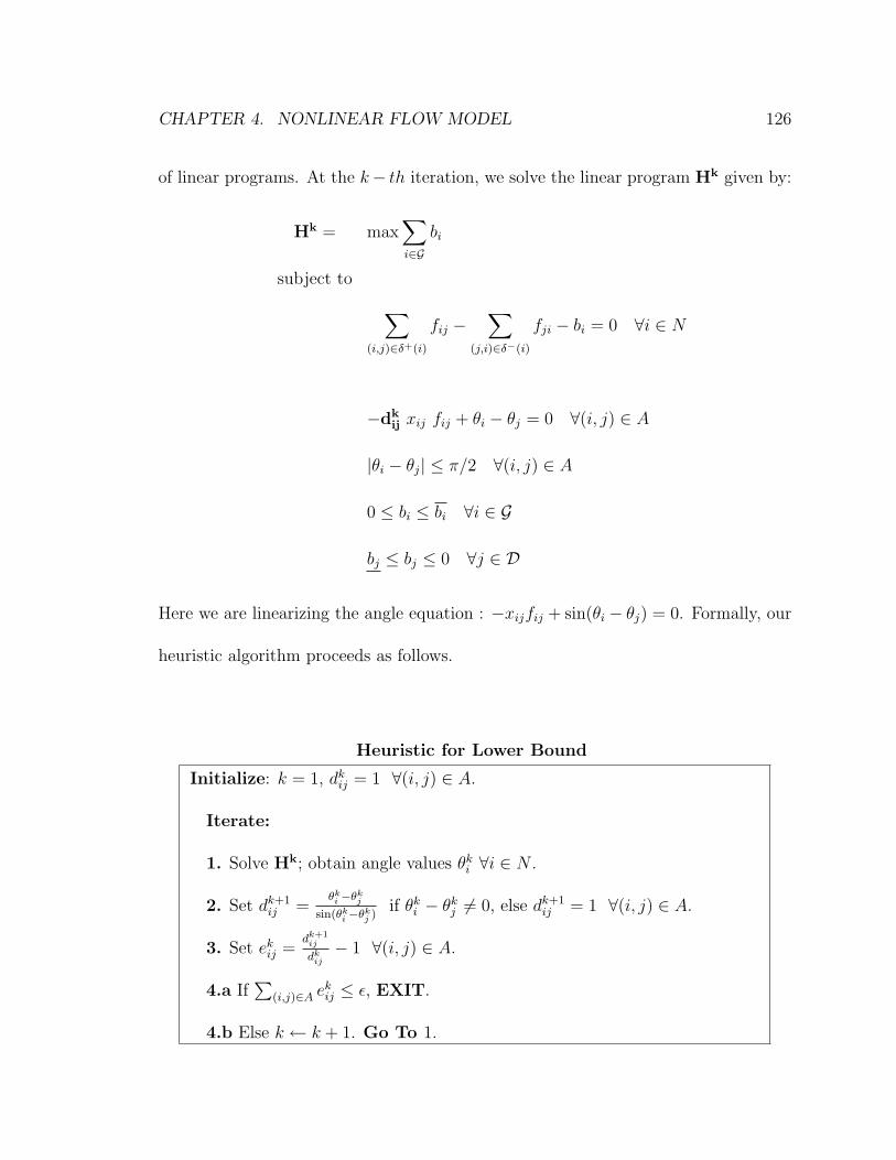
CHAPTER 4. NONLINEAR FLOW MODEL 126
of linear programs. At the k− th iteration, we solve the linear program Hk given by:
Hk = max∑i∈G
bi
subject to ∑(i,j)∈δ+(i)
fij −∑
(j,i)∈δ−(i)
fji − bi = 0 ∀i ∈ N
−dkij xij fij + θi − θj = 0 ∀(i, j) ∈ A
|θi − θj| ≤ π/2 ∀(i, j) ∈ A
0 ≤ bi ≤ bi ∀i ∈ G
bj ≤ bj ≤ 0 ∀j ∈ D
Here we are linearizing the angle equation : −xijfij + sin(θi − θj) = 0. Formally, our
heuristic algorithm proceeds as follows.
Heuristic for Lower Bound
Initialize: k = 1, dkij = 1 ∀(i, j) ∈ A.
Iterate:
1. Solve Hk; obtain angle values θki ∀i ∈ N .
2. Set dk+1ij =
θki −θk
j
sin(θki −θk
j )if θki − θkj 6= 0, else dk+1
ij = 1 ∀(i, j) ∈ A.
3. Set ekij =dk+1
ij
dkij− 1 ∀(i, j) ∈ A.
4.a If∑
(i,j)∈A ekij ≤ ε, EXIT.
4.b Else k ← k + 1. Go To 1.

CHAPTER 4. NONLINEAR FLOW MODEL 127
We believe that the lower bound heuristic besides providing a valid lower bound
would specially be useful on very big networks (with several thousand arcs) where
IPOPT may not scale very well.
Table 4.1 summarizes the results of our testing with different networks. For all
networks we scaled demand and supply vectors by total demand, so the maximum
demand that can be satisfied is 1. The first column gives the size of network, the
column L1 gives the lower bound obtained by solving TP using IPOPT while L2 gives
that obtained by our heuristic. The column U gives the upper bound obtained by
solving the LP-relaxation to the dual problem while the last column gives the duality
gap between the best found lower bound and upper bound. In each column the value
in parenthesis is the time taken in seconds.
From the results, we see that the “duality” gap is quite low for most instances.
The algorithm also scales well as the network size increases. The time taken to solve
an instance is extremely small ranging from fraction of seconds for small networks to
a few seconds on the big networks.
4.6 Capacitated Nonlinear Flow Model
In the previous section we considered throughput maximization problem when the
underlying flow model is nonlinear. In this section we consider a slight generaliza-

CHAPTER 4. NONLINEAR FLOW MODEL 128
Table 4.1: Computational Results
Network Size L1 L2 U % gap
13 nodes, 30 arcs 0.77180 (0.01) 0.77180 (0.01) 0.77914 (0.00) 0.951 %
49 nodes, 84 arcs 0.54800 (0.02) 0.54787 (0.03) 0.55911 (0.02) 2.027 %
98 nodes, 204 arcs 0.77345 (0.04) 0.77282 (0.13) 0.79076 (0.13) 2.236 %
300 nodes, 409 arcs 0.76749 (0.10) 0.76736 (0.19) 0.76813 (0.12) 0.083 %
600 nodes, 990 arcs 0.55429 (0.45) 0.55397 (0.68) 0.55999 (3.43) 1.028 %
649 nodes, 1368 arcs 0.67272 (1.22) 0.66756 (1.44) 0.67692 (6.94) 0.624 %
tion to the problem considered in the previous section. We look at the throughput
maximization problem when the underlying flow model is nonlinear with the addi-
tional constraint that flow on every arc is within pre-specified capacity. Intuitively,
the capacitated version of the throughput maximization problem seems like a minor
modification to the uncapacitated one, but as we shall see, is considerably difficult in
terms of finding good global solutions.
4.6.1 Model Description
We begin by specifying the model. As before, fij indicates power flow on arc (i, j), θi
represents “phase angle” at node i, while bi denotes net supply emanating from node

CHAPTER 4. NONLINEAR FLOW MODEL 129
i. The set of feasible power flows and phase angles consists of the solutions to the
following system (CFEAS):
CFEAS :∑
(i,j)∈δ+(i)
fij −∑
(j,i)∈δ−(i)
fji = bi ∀i ∈ N (4.36)
sin(θi − θj)− xijfij = 0 ∀(i, j) ∈ A (4.37)
| fij | ≤ uij ∀(i, j) ∈ A (4.38)
| θi − θj | ≤π
2∀(i, j) ∈ A (4.39)
As before, constraint (4.36) models flow conservation, while (4.37) describes angle-
equations. Constraint (4.38) specifies maximum flow permissible for each arc while
(4.39) is required for steady state stability of the system. Observe that the system
CFEAS reduces to the system FEAS((4.1)-(4.3)) if the capacity of every arc is
greater than the inverse of resistance for the arc, i.e., uij ≥ 1/xij for all arc (i, j).
Also, we note that the function sin−1 has range [−π/2, π/2]; consequently (4.37)
(4.39) and (4.38) can simply be replaced by the constraints
θi − θj = sin−1(xijfij), |θi − θj| ≤ θij (4.40)
where θij = sin−1(min{1, xijuij}). Hence instead of capacity constraints (4.38) one
can alternatively specify “phase” angle bound constraints for each arc (i, j) which
can be represented by (4.40). Before going further, we define the set Sβ.

CHAPTER 4. NONLINEAR FLOW MODEL 130
Definition 4.6.1 Let N be the node-arc incidence matrix for the network and con-
sider the diagonal matrix X ∈ Rm×m = diag(xij). The vector θ ∈ Rm is the vector
of all angle bounds θij given by (4.40). We define the set of feasible supply-demand
vectors Sβ as follows:
Sβ := {b ∈ Rn | ∃ (f, θ) ∈ Rm+n : Nf − b = 0,
− sin−1(Xf) +NT θ = 0, | NT θ | ≤ θ } (4.41)
We further define the set of feasible supply vector SGβ as the set Sβ restricted to the
generator nodes G.
Let G be the set of generator nodes and D be the set of demand nodes while bi be
the maximum supply for generator node i ∈ G and −bj be the maximum demand for
demand node j ∈ D. Similar to the uncapacitated version, we define the throughput
maximization problem as following:
CTP : max.∑i∈G
bi
s.t. b ∈ Sβ
0 ≤ bi ≤ bi ∀i ∈ G
bj ≤ bj ≤ 0 ∀j ∈ D
Theorem 4.6.2 The capacitated version of throughput maximization problem (CPT)
is NP-hard.

CHAPTER 4. NONLINEAR FLOW MODEL 131
Proof. See Chapter 5.1.
Non-Monotonicity
Now we try to motivate why the capacitated version of throughput maximization
problem is difficult. The system of equations is highly nonlinear and non-convex, so
we can not hope for an algorithm which will perform exceedingly well on all instances.
Moreover, we will show by means of an example that the set Sβ can also be disjoint.
This leads to disjunctions in the space of decision variables b (demand-supply vector).
We believe this is the primary source of difficulty for solving the capacitated version
of throughput maximization problem.
Consider the example in Figure 4.1: the network has 5 nodes and 6 arcs, with one
source (node 0) and one sink (node 4). The resistances for arcs (0, 2) and (2, 4) are
2.50 and 4.00 respectively, while all other arcs have resistance of 1. The capacity of
arc (1, 2) is 0.005 while capacity for any other arc (i, j) is chosen such that xijuij = 1.
We solve CFEAS given by (4.36)-(4.39) for different demand-supply values. While
solving CFEAS we first ignore flow capacity constraints (4.38) to get unique value
of flow for each arc. We then check if flow on any arc is above capacity. If that
is the case then CFEAS is not feasible for current demand-supply value, otherwise
CFEAS is feasible with flows as computed without capacity constraints. Since our
example has a single generator and demand node, the demand-supply value is same

CHAPTER 4. NONLINEAR FLOW MODEL 132
0
3
4
2
1x_13 = u_13 = 1
x_01 = u_01 = 1
x_24 = 4u_24 = 0.25
x_02 = 2.5u_02 = 0.4
x_34 = u_34 = 1
x_12 = 1u_12 = 0.005
Figure 4.1: Non-monotone example.
0 0.1 0.3 0.4 0.5 0.6 0.7 1 0.156 0.783 0.8807 0.951−0.02
−0.015
−0.01
−0.005
0
0.005
0.01
0.015
Figure 4.2: Flow on arc (1, 2) v Throughput.

CHAPTER 4. NONLINEAR FLOW MODEL 133
as throughput.
Figure 4.2 presents flow on arc (1, 2) for different throughput values (computed
without enforcing capacity constraints). From the plot it is evident that the flow on
arc (1, 2) behaves in a non-monotonous fashion. Initially the flow increases (and is
positive) but eventually decreases and changes sign as throughput value increases.
Finally we apply capacity constraint (4.38) to get values of throughput for which the
flow is within capacity. The set of feasible supply value is highlighted in the plot and
is given by :
SGβ = [0, 0.156] ∪ [0.783, 0.8807] (4.42)
In this example, the set of feasible supply values SGβ as defined in Definition 4.6.1
is disjoint. This leads to disjunctions in the space of decision variables b (demand-
supply vector). One can easily come up with examples where the feasible region is a
collection of discrete points and continuous regions. The resolution of this disjunction
requires either branching or Integer Programming based techniques.

Chapter 5
NP-completeness proof
This section outlines the proof for Theorem 4.6.2. Also refer to remark 5.1.6 at the
end of the proof.
5.1 Proof of Theorem 4.6.2
We will use the following problem for NP-hardness proof.
Problem 5.1.1 We are given m clauses C1, . . . , Cm involving n Boolean variables
x1, . . . , xn where each clause Ci has exactly three variables. The one-in-three 3-
SAT problem is to determine whether there exists a truth assignment to the variables
so that each clause has exactly one true literal (and thus exactly two false literals).
Given an instance of the Problem 5.1.1 we will transform it into an instance of our
capacitated throughput maximization problem. Before that we need to define some
134

CHAPTER 5. NP-COMPLETENESS PROOF 135
terms and introduce notations.
We define the “banana” network as following : Consider the network described
by Figure 5.1: the network has 6 nodes and 7 arcs, with one source (node 0) and one
sink (node 5). The resistances for arcs (0, 2) and (2, 4) are 2.50 and 4.00 respectively,
while all other arcs have resistance of 1. The capacities of arcs (1, 2) and (4, 5) are
0.005 and 0.783 respectively, while capacity for any other arc (i, j) is chosen such
that xijuij = 1. The network is similar to the one described by Figure 4.1 but has an
additional arc ((4, 5)) and an extra node (5).
0
3
4
2
1x_13 = u_13 = 1
x_01 = u_01 = 1
x_24 = 4u_24 = 0.25
x_02 = 2.5u_02 = 0.4
x_34 = u_34 = 1
x_12 = 1u_12 = 0.005
5x_45 = 1
u_45 = 0.783
Figure 5.1: “Banana” network.
Lemma 5.1.2 The set of feasible supply values (as defined by 4.6.1) for the “banana”
network is given by SGβ = [0, 0.156] ∪ {0.783}.
Proof. From (4.42) the set of feasible supply values for the network described by
Figure 4.1 is [0, 0.156] ∪ [0.783, 0.8807]. The “banana” network is same as the one
described by Figure 4.1 other than the presence of an additional arc and node. Since

CHAPTER 5. NP-COMPLETENESS PROOF 136
the extra arc (4, 5) is the only arc incident to the sink node 5, the throughput of
the “banana” network is bounded by the capacity of this arc which is 0.783. Hence
SGβ = [0, 0.156] ∪ {0.783} for the “banana” network.
For the rest of the proof we define F := 0.156 and G := 0.783 as the lower and upper
threshold values of throughput in the “banana” network. Hence, for the “banana”
network SGβ = [0, F ] ∪ {G}.
For each variable in the one-in-three 3-SAT problem 5.1.1, we define a “variable”
network (Figure 5.2) as following : Take two copies of the “banana” network and
connect their sinks with a super-sink. The capacity of arcs incident to the super-
sink is “large” while the resistance of these arcs is “small”, so that these arcs are
never critical in any throughput maximization problem. The maximum demand at
super-sink is F +G while the maximum supply at each of the two sources is G.
Figure 5.2 describes the “variable” network: B-upper and B-lower refer to the two
copies of the “banana” network, node t is the super-sink while nodes s1 and s2 are
the two sources.
Lemma 5.1.3 When the throughput value of the “variable” network is F +G, one of
its component “banana” network carries a flow of exactly F while the other component
carries a flow of exactly G.

CHAPTER 5. NP-COMPLETENESS PROOF 137
s1
s2
t
B−lower
B−upper
F+G
G
G
Figure 5.2: “Variable” network.
Proof. Let x and y denote the flows on the component “banana” networks. From
Lemma 5.1.2 we know that the flows on component “banana” networks lie in a dis-
continuous interval, i.e., x, y ∈ [0, F ]∪{G}. Since throughput is F +G, we must have
x+y = F +G. The result follows immediately by using the above two in conjunction.
Next we define a “clause” network for every clause in the one-in-three 3-SAT problem
5.1.1. We take three copies of the “banana” network and connect their sinks with a
super-sink. Each copy of the “banana” network refers to one of the three literals in
the clause. As with the “varaible” network the capacity of arcs incident to the super-
sink is “large”while the resistance of these arcs is “small”. The maximum demand at
super-sink is F + 2G while the maximum supply at each of the three sources is G.
Figure 5.3 describes the “clause” network. There is one “banana” network for
each literal in the clause.

CHAPTER 5. NP-COMPLETENESS PROOF 138
s1
t
s3G
G
G
F+ 2Gs2
Figure 5.3: “Clause” network.
Lemma 5.1.4 When the throughput value of the “clause” network is F + 2G, one
of its component “banana” network carries a flow of exactly F while the other two
components carry flow of G each.
Proof. Same as the proof of Lemma 5.1.3.
Now we define the “linking” arcs which will transform any instance of Problem 5.1.1
to our problem. For each clause we do the following:
• If a variable occurs as a positive literal we introduce two arcs : The first (second)
arc connects the left-most (right-most) node of “banana” network corresponding
to the given variable in the “clause” network with the left-most (right-most) node
of the upper “banana” network in the “variable” network. This is illustrated in
Figure 5.4.
• If a variable occurs as a negative literal we again introduce two arcs : The

CHAPTER 5. NP-COMPLETENESS PROOF 139
first (second) arc connects the left-most (right-most) node of “banana” network
corresponding to the given variable in the “clause” network with the left-most
(right-most) node of the lower “banana” network in the “variable” network.
The capacity for every “linking” arc is 0 while the resistance for every such arc is
1. We will refer to the pair of “banana” networks between every clause and variable
as “parallel” sub-networks. In Figure 5.4 the “banana” networks denoted by B-upper
and x1 are “parallel”.
B−lower
B−upper
Variable x_1
x_1
x_2
~x_3
G
G
G
G
G
Clause c1 :
x_1 + x_2 + ~x_3
F+G
F+2G
Figure 5.4: Linking Arcs.
This completes the transformation of any instance of one-in-three 3-SAT to an in-
stance of our problem, we call the network so obtained as the “transformed” network.

CHAPTER 5. NP-COMPLETENESS PROOF 140
Clearly the transformation was done in polynomial size in the input data.
Lemma 5.1.5 Any instance of one-in-three 3-SAT to our problem is satisfiable if
and only if the maximum throughput value in the “transformed” network is n(F +
G) +m(F + 2G).
Proof. Suppose the maximum throughput value is n(F + G) + m(F + 2G). The
“transformed” network has n + m demand nodes, one for each clause and variable.
The maximum demand value at a demand node corresponding to a variable is F +G
while the same for a demand node corresponding to a clause is F + 2G. Since the
throughput value is n(F + G) + m(F + 2G) every demand node is being served its
maximum demand value.
Since the capacities of arcs connecting the “variable” and “clause” network is zero,
no amount of flow is transmitted between the two. Now, using Lemmas 5.1.3 and
5.1.4, we have that for every “variable” network one component carries a flow of F
and the other carries a flow of G while for every “clause” network one component
carries a flow of F and the other two carry flow of G.
Now we insist that the flow in optimal solution must have the following struc-
ture : the flow on the two components of “parallel” sub-network is same for every
such “parallel” sub-network in the “transformed” network. This is illustrated by
the following argument. Since the capacities of arcs connecting the components of
“parallel” sub-network is zero, no amount of flow is transmitted between the two.

CHAPTER 5. NP-COMPLETENESS PROOF 141
Moreover, by applying Ohm’s Law (4.40), we must have that the angle difference
between the two components of “parallel” sub-network is same. Hence the flows on
the two components of “parallel” sub-network must be same.
Now we obtain a Boolean assignment by the following rule : We define the value
of Boolean variable to be TRUE if and only if the in the “variable” network, the flow
on the upper “banana” network is F and flow on the lower “banana” network is G.
We will show that the assignment so obtained is satisfiable. In each “clause” net-
work, the literal with flow F corresponds to TRUE assignment while those with flow
G correspond to FALSE assignments. Hence there is exactly one TRUE assignment
and exactly two FALSE assignments.
Lets consider the case when a negative literal is given a TRUE assignment, which
means that the corresponding variable should assume a FALSE assignment. For a
negative literal the “parallel” sub-network is obtained by connecting the end-points
of the lower “banana” network in the “variable” network to that in the “clause”
network. Since the negative literal is TRUE the corresponding “banana” network in
the “clause” network as well as the lower “banana” network in the variable network
will carry a flow of F , hence the upper “banana” network in the “variable” network
must carry a flow of G. Hence, from the rule defined above, the corresponding
variable will be given an assignment of FALSE. Hence the rule is consistent with
the assignment that was anticipated. Similar results can be easily shown for the
remaining cases.

CHAPTER 5. NP-COMPLETENESS PROOF 142
The other way round can be proved similarly by starting with the assignment rule
and then following steps in reverse order.
Remark 5.1.6 Figure 4.2 that we plotted before showed flow on arc (1, 2) as a func-
tion of throughput of the network (described by figure 4.1). There are two basic prob-
lems with the proof:
(1) In the proof, we need to assume that f12, as a function of throughput, has the
desired structure between the two points where the curve crosses the horizontal
line (at the capacity u12). That is to say, we need to assume that the curve first
increases monotonely, and then decreases monotonely. However, we plotted
figure 4.2 by sampling several values of throughput and calculating f12 at those
values.
(2) In fact, the two points where the curve crosses the horizontal line probably have
irrational values, so we cannot express them exactly in the NP-completeness
proof.
Of the two problems, (2) is the harder one, but actually we can fix them both at once.
The following result does the job.
Before we show the result, lets introduce some notation : Given a solution (f, θ),
let us denote by T (f, θ), or T for short, the throughput, i.e. f01 + f02. Lets also
denote the angle difference between two nodes i and j by θij, i.e. θij = θi − θj.

CHAPTER 5. NP-COMPLETENESS PROOF 143
Theorem 5.1.7 For any ε > 0 there exists δ > 0 with the following property: if (f, θ)
and (f , θ) be feasible solutions with T (f, θ) < T (f , θ) < T (f, θ)+δ, then |f12−f12| ≤ ε.
Proof. We will assume that δ > 0 is given and will show later how to choose it as
a function of ε. So assume that T (f, θ) < T (f , θ) < T (f, θ) + δ. Without loss of
generality assume θ0 = θ0. Since T (f, θ) < T (f , θ) we must have θ1 < θ1 or θ2 < θ2,
or both.
Assume first that θ1 < θ1 and θ2 ≥ θ2 ( the symmetric case, θ1 ≥ θ1 and θ2 ≤ θ2,
is identical and will be skipped).
Since θ21 > θ21, we have f21 > f21. Also, f01 > f01. So f13 > f13 and θ13 > θ13,
and θ3 < θ3. Similarly, f34 > f34, and so θ34 > θ34, and θ4 < θ4. Thus thus θ24 > θ24,
and f24 > f24.
Now, T (f , θ) = f24 + f13 = f24 + f01 + f21 > f24 + f01 + f21 = T (f, θ) + f21− f21.
So, f21 < f21 < f21 + δ.
Assume next that θ1 < θ1 and θ2 < θ2. Then for i = 1, 2, f0i < f0i, and so
f0i < f0i < f0,i + δ, and using the second-order Taylor approximation,
θ0i ≤ θ0i + O(δ1/2)
(when |θ0i| is near π/2 the first-order term goes to zero), and so
|θi − θi| ≤ O(δ1/2).

CHAPTER 5. NP-COMPLETENESS PROOF 144
From this we obtain:
|f21 − f21| ≤ O(δ1/2).
Using δ = O(ε2) the theorem follows.
We constructed the curve in figure 4.2 by sampling on a fine grid. The theorem
shows that the actual functional value can differ from what the curve shows, but only
by very small amounts. This allows the NP-completeness proof to go through.

Bibliography
[1] R. K. Ahuja, T. L. Magnanti, and J. B. Orlin. Network Flows: Theory, Algo-
rithms, and Applications. Prentice Hall, NJ (1993).
[2] S. Boyd and L. Vandenberghe, Convex Optimization, Cambridge University
Press (2004).
[3] G. Andersson, Modelling and Analysis of Electric Power Systems. Lecture 227-
0526-00, Power Systems Laboratory, ETH Zurich, March 2004. Download from
http://www.eeh.ee.ethz.ch/downloads/academics/courses/227-0526-00.pdf.
[4] J. Salmeron, K. Wood, and R. Baldick, Analysis of Electric Grid Security Under
Terrorist Threat, IEEE Trans. Power Systems 19 (2004), 905–912.
[5] R. Alvarez, Interdicting Electric Power Grids, Masters’ Thesis, U.S. Naval Post-
graduate School, 2004.
145

BIBLIOGRAPHY 146
[6] J. Arroyo and F. Galiana, On the Solution of the Bilevel Programming Formu-
lation of the Terrorist Threat Problem, IEEE Trans. Power Systems, Vol. 20
(2005), 789–797.
[7] D. Bienstock and S. Mattia, Using mixed-integer programming to solve power
grid blackout problems , Discrete Optimization 4 (2007), 115–141.
[8] A. Pinar, J. Meza, V. Donde, and B. Lesieutre, Optimization Strategies for
the Vulnerability Analysis of the Power Grid, submitted to SIAM Journal on
Optimization (2007).
[9] V. Donde, V. Lopez, B. Lesieutre, A. Pinar, C. Yang, and J. Meza, Identification
of severe multiple contingencies in electric power networks, Proceedings of the
37th North American Power Symposium, Ames, Iowa (2005).
[10] A.Pinar, A. Reichert, and B.Lesieutre, Computing Criticality of Lines in Power
Systems, Lawrence Berkeley National Laboratory. Paper LBNL-61763 (2006).
[11] B. Lesieutre, A. Pinar, and S. Roy, Power system extreme event detection: The
vulnerability frontier, Proc. 41st Hawaii International Conference on System
Sciences, Hawaii (2008).
[12] B. Lesieutre, S. Roy, V. Donde, and A. Pinar, Power sytem extreme event screen-
ing using graph partitioning,Proceedings of the 38th North American Power Sym-
posium, Carbondale, Illinois (2006).

BIBLIOGRAPHY 147
[13] J.F. Benders, Partitioning procedures for solving mixed variables programming
problems, Numerische Mathematik 4 (1962), 238–252.
[14] D. Braess, Uber ein Paradox der Verkerhsplannung, Unternehmenstorchung Vol.
12 (1968) 258–268.
[15] ILOG CPLEX 11.0. ILOG, Inc., Incline Village, NV.
[16] H. Y. Benson, D. F. Shanno, and R. J. Vanderbei, Interior-point methods for
nonconvex nonlinear programming: jamming and comparative numerical testing,
Math. Programming 99, 35 – 38 (2004).
[17] Vanderbei, R. 1997. LOQO User’s manual, Statistics and Operations Research
Technical report No SOR-97-08, Princeton University.
[18] R. Fletcher, N. I. M. Gould, S. Leyffer, Ph. L. Toint, and A. Wachter, Global
convergence of trust-region SQP-filter algorithms for general nonlinear program-
ming, SIAM J. Optimization 13, 635–659 (2002).
[19] A. Wachter and L. T. Biegler, On the Implementation of a Primal-Dual Inte-
rior Point Filter Line Search Algorithm for Large-Scale Nonlinear Programming,
Mathematical Programming 106, 25–57, (2006).
[20] The IEEE reliability test system–1996, IEEE Trans. Power Syst., vol. 14 (1999)
1010 - 1020.

BIBLIOGRAPHY 148
[21] S.T. DeNegre and T.K Ralphs, A Branch-and-cut Algorithm for Integer Bilevel
Linear Programs, COR@L Technical Report, Lehigh University (2008).
[22] U. Janjarassuk and J. T. Linderoth, Reformulation and Sampling to Solve a
Stochastic Network Interdiction Problem, to appear, Networks (2008).
[23] C. Lim and J.C. Smith, Algorithms for Discrete and Continuous Multicommodity
Flow Network Interdiction Problems, IIE Transactions 39, 15-26, 2007.
[24] S. Boyd, Convex Optimization of Graph Laplacian Eigenvalues, Proc. Interna-
tional Congress of Mathematicians 3 (2006), 1311–1319.
[25] B. Mohar, The Laplacian spectrum of graphs, in: Y. Alavi, G. Chartrand, O.
Oellermann, A. Schwenk (Eds.), Graph Theory, Combinatorics, and Applica-
tions, London Math. Soc. Lecture Notes, Wiley-Interscience, 871-898 (1991).
[26] B. Carreras, V. Lynch, I. Dobson, and D. Newman, Dynamics, criticality, and
selforganization in a model for blackouts in power transmission systems, Proc.
35th Hawaii International Conference on System Sciences, Hawaii (2002).
[27] B. Carreras, V. Lynch, M. Sactjen, I. Dobson, and D. Newman, Modeling black-
out dynamics in power transmission networks with simple structure, Proc. 34th
Hawaii International Conference on System Sciences, Maui, Hawaii (2001).

BIBLIOGRAPHY 149
[28] I. Dobson, B. Carreras, V. Lynch, and D. Newman, An initial model for complex
dynamics in electric power system blackouts, Proc. 34th Hawaii International
Conference on System Sciences, Maui, Hawaii (2001).
[29] Dynamical and probabilistic approaches to the study of blackout vulnerability
of the power transmission grid, Proc. 37th Hawaii International Conference on
System Sciences, Hawaii (2004).
[30] I. Dobson, J. Chen, J. Thorp, B. Carreras, and D. Newman, Examining criticality
of blackouts in power system models with cascading events, Proc. 35th Hawaii
International Conference on System Sciences, Hawaii (2002).
[31] I. Dobson, K. Wierzbicki, B. Carreras, V. Lynch, and D. Newman, An estimator
of propagation of cascading failure, Proc. 39th Hawaii International Conference
on System Sciences, Hawaii (2006).
[32] G. Oliviera, S. Binato, L. Bahiense, L. Thome, and M. Pereira, Security-
constrained tranmission planning: a mixed-integer disjunctive approach, Op-
timization Online (2004).
[33] J. F. Bard, Practical Bilevel Optimization: Algorithms and Applications, Kluwer
Academic Publishers (1998).
[34] H. Von Stackelberg, The Theory of Market Economy, Oxford University Press,
Oxford (1952).

BIBLIOGRAPHY 150
[35] U.S.-Canada Power System Outage Task Force, Final Report on the August 14,
2003 Blackout in the United States and Canada: Causes and Recommendations,
April 5, 2004. Download from: https://reports.energy.gov.
[36] Electric Consumer Research Council (ELCON), The Economic Impacts of the
August 2003 Blackout, February 2004.