potential flows

The Use of MathCad in Teaching IdealFluid Flow with Complex Variables*

MICHAEL REX MAIXNERMaine Maritime Academy, Castine, Maine ME, USA. E-mail: [email protected]

The use of MathCad for the visualization of two-dimensional, irrotational, steady, incompressibleflow patterns is discussed, along with the appropriate mathematical background. MathCad'scontour plotting capabilities and its ability to handle complex numbers permit rapid depiction ofbasic flows and linear combinations of these flows with relative ease, allowing students toconcentrate on understanding the material and broader concepts. Sample output, recommendedlecture topics, and suggested topics for further study are presented, and the address of a web sitecontaining a prepared lecture is provided (http://www.mathsoft.com/appsindex.html).

NOMENCLATURE

a cylinder radiusf complex function used in definition of

Milne-Thompsoncircle theorem (see text)F � �� i , complex potential

F 0 � dF

dz� uÿ iv, complex velocity

�F 0 � u� iv, velocityi � ��ÿ1

p(Note the carat (^) atop the letter

i to differentiate it from the letter i whenemployed as a subscript or index.)

i index associated with x-directionj index associated with y-directionn number of subdivisions in x- and y-

directionsQ array of source and sink strengths in von

KaÂrmaÂn problem (see text)r � jzj �

��x2 � y2

p, modulus of position

in the complex planeUo magnitude of free stream velocityu velocity in the x-directionv velocity in the y-directionV � jF 0j � j�F 0j, magnitude of velocityx real component of position in the

complex planeX array of source and sink locations in von

KaÂrmaÂn problem (see text)y imaginary component of position in the

complex planez � x� iy � rei�, position in the complex

plane� orientation angle of free-stream relative

to positive x-axis� orientation angle of doublet relative to

positive x-axisÿ vortex strength� angle of position in the complex plane,

measured counter-clockwise from posi-tive x-axis

� source (or sink) strength� doublet strength� = Re(F), potential function = Im(F), stream function

INTRODUCTION

FLOW VISUALIZATION has been an invaluabletool in the study of ideal and real fluid flows,providing a synergism that allows the student togain an understanding not only of the phenomen-ological aspects of the flow, but also of the under-lying mathematics. Detailed analysis of these flowvisualizations permits not only the streamline andequipotential patterns to be obtained, but also thelocation of critical points in the flow, such asstagnation points. Numerous methods of flowvisualization exist, and include electric analogs,experimental techniques (hydrogen bubblemethod, smoke tunnels, aluminum flakes sprinkledon the surface of dye-colored water, dye injection,etc. [1, 2]). Given the requisite time and patience,qualitative sketches of potential flow patternsprovide additional insight into the underlyingphysics. A natural outgrowth of sketches is theuse of computer graphics to assist in these visual-izations, but early attempts at the use of computersfor this purpose were generally limited to main-frame machines with, eventually, time-sharingworkstations with graphics terminals [3±6]. Morerecent developments in flow visualization withpersonal computers are provided in the references[7±9]. MathCad, a relatively inexpensive and read-ily available calculation software product, com-bines an excellent contour plotting capability andthe ability to perform calculations with complexfunctions. This makes it an extremely powerfultool in the visualization of ideal fluid flow patternsby individual users on personal computers.* Accepted 6 June 1999.

456

Int. J. Engng Ed. Vol. 15, No. 6, pp. 456±468, 1999 0949-149X/91 $3.00+0.00Printed in Great Britain. # 1999 TEMPUS Publications.

Students with a background in basic fluidmechanics and complex variables are quickly ableto obtain plots of streamlines and equipotentiallines.

At Maine Maritime Academy, the course`Numerical and Computer Methods for Engineer-ing Design' (Es490) is taken in the spring term ofthe third year of a five-year marine engineeringsystems curriculum. Prior to that, students havehad basic courses in fluid mechanics and struc-tured computer programming, and will also havebeen introduced to complex variables. Es490 alsofollows an introductory design course, and istaken in conjunction with an intermediate designcourse. The course provides students with a varietyof numerical methods and techniques (numericalintegration, differentiation, finite differencemethods, interpolation, curve fitting, solution ofdifferential equations and systems of differentialequations, etc.) that may be used throughoutthe remainder of their curriculum, including thetwo-semester capstone design sequence taken inthe fifth year. Excel spreadsheets, QBASIC,and MathCad are utilized to complete a varietyof problems (structural, electrical, fluid mech-anics, optimization, aerodynamics, heat transfer,etc.).

As part of this course, students receiveinstruction in the representation of ideal fluidflows as a complex function whose real andimaginary parts are, respectively, the potentialand stream functions. Following this basicinstruction and several examples, students arerequired to solve problems involving linearcombinations of these potential flows, to drawelementary conclusions from these representa-tions, and, in general, to recognize the powerof this method, especially when used in conjunc-tion with boundary layer methods at fluid-structure interfaces. The prototype of thisinstructional method was employed in theearly 1980s by the author when on the facultyof the Department of Mechanical Engineeringat the Naval Postgraduate School in Monterey,California. At that time, an IBM 360 main-frame was required to run the program, withstudents utilizing time-sharing stations and separ-ate Tektronix graphics screens to view the flowpatterns. With the advent and proliferation ofpersonal computers and software since then, thesame capability is now available on desktop andlaptop computers. The intent of this instructionalpackage (originally at the Naval PostgraduateSchool and in its current incarnation at MaineMaritime Academy) was to relieve students ofthe laborious plotting associated with flow visual-ization. The student is thus able to investigatemany more combinations of basic potential flowsand, consequently, obtain a better understandingof the subject matter. It is this method and itsspecific implementation in Es490 at Maine Mari-time Academy with which the remainder of thisarticle is concerned.

BACKGROUND

Students who took the pilot version of Es490 inthe fall of 1998 and spring of 1999 were required topurchase the student edition of MathCad, version7. The professional edition of MathCad was alsoavailable for both classroom instruction and after-hours use on the local-area network. The topic ofpotential flows is presented in the latter part of theterm, so students will already be familiar withMathCad when this subject is reached.

A detailed lesson plan file in MathCad work-sheet format is provided to all students to followalong during the lectures and to use as a studyguide. A copy of the lesson plan may be obtainedthrough the MathCad web site or directly from theauthor by e-mail. Due to the number of illus-trations embedded in the lesson plan and the gridsize used for illustrations, it is recommended thatthe program be run on a computer with at least aPentium processor, otherwise the refresh times forsuccessive screens becomes excessively long. Alter-natively, the grid coarseness may be increased byreducing the number of grid points (see nextsection) with a concomitant reduction in graphicquality.

The background for this topic may be found invarious mathematics [10,11] and fluid mechanics[12] texts; many of the details are omitted here forthe sake of brevity, but may be found in the lessonplan placed on the MathCad web site. Instructionbegins with a review of the basics of complexnumber theory, whereby an imaginary number, z,may be represented in either rectangular (x- and y-components) or polar (r- and �-components):

z � x� iy � rei� � r�cos �� i sin �� 1�where � = arctan (y/x).

For the two-dimensional, irrotational, steadyflow of an incompressible fluid, the u- and v-components of velocity (in the x- and y-directions,respectively) are related by the Cauchy-Riemannequations:

v � ÿ @ @x� @�@y

�2�

u � @ @y� @�@x

:

where � and are, respectively, the equipotentialand stream functions for the flow; they are ortho-gonal, and give rise to the complex potentialfunction:

F�z� � ��x; y� � i �x; y� �3�Most students readily grasp the significance of astreamline (a line of constant ) and recognizethat there can be no velocity normal to a stream-line. The concept of an equipotential (a line ofconstant �) is usually not as easily mastered, andmust be reinforced through the correlation of the

The Use of MathCad in Teaching Ideal Fluid Flow with Complex Variables 457

Cauchy-Riemann equations with plots of equi-potential lines in ideal flow patterns.

The student is then shown that the complexvelocity may therefore be obtained from:

F 0�z� � dF

dz� @F

@x� @�

@x� i

@

@x� uÿ iv �4�

MathCad's built-in derivative function may beemployed in this last equation. Note that inorder to obtain the actual velocity, we must take:

�F 0�z� � u� iv �5�Finally, the magnitude of the velocity may beobtained from:

V�z� � jF 0�z�j � j�F 0�z�j � ��F 0 � F 0j1=2 � �u2 � v2�1=2

�6�

DISCRETIZATION OF FLOW FIELD

Prior to displaying any of the more interestingpotential flows, a grid must be established, with thegrid intersections being the points at which � and will be calculated. A grid is employed with x andy each bounded by �1.5, with the domain sub-divided into a number of rectangles in the x- and y-directions. All grid points are then offset slightlyby the same amount xoffset = yoffset = 0.0001;should the user decide to place a singularity at,say, z � 0� i0, (a common choice), then calcula-tion will not be performed `at' the singularity. Thisshift is essentially transparent to the user from thispoint on. An equal number of grid points isutilized in each direction, with indices in the x-and y-directions, respectively, of i � 0! n andj � 0! n; with n � 25, this gives, in all, (n + 1)2 =676 points in the plotting area. MathCad's defaultindex counter is set to 0 so that all vector and matrixsubscripts begin with 0; the grid point corres-ponding to i = 0, j = 0 is situated at the lower leftcorner of the plotting area.

The complex offset zoffset and complex grid-points zi,j are defined as:

zoffset � xoffset � iyoffset �7�

xi � xmin � i � �xmax ÿ xmin�n

yj � ymin � j � �ymax ÿ ymin�n

zi;j � zoffset � �xi � iyj�(The choice of zoffset and the grid size (i.e., n) mayresult in large values of F(z), depending on howclose a grid intersection lies to the location of asingularity. Since MathCad may arbitrarily selectthe contour values, adjacent contours may thenappear very dense or very sparse. The user may berequired to make judicious choices of n and thelocation of singularities to produce suitablecontour density.)

Once the grid is established and and/or � areevaluated at each grid point, MathCad's contourplotting capability is used to plot or �. MathCadperforms a linear interpolation between gridpointsto establish contours of the quantity being plotted(either � or ); the �ij or ij are stored as a matrixof equally spaced values, without reference to thecoordinates at which � or are evaluated. Thedefault plotting limits for grid positions areÿ1 � x � 1 and ÿ1 � y � 1, and must be changedby the user to reflect the values previously chosen(i.e., xmin � x � xmax and ymin � y � ymax).

Version 7 of MathCad limits the user to onecontour plot per graph. If, instead, two contourplots were allowed, then lines of constant � andlines of constant could be viewed on the sameplot, thereby illustrating the orthogonality of thesetwo functions. Instead, the user must plot � and on separate graphs; if placed in close proximity toone another, though, the orthogonality is readilydiscernable. MathCad Version 8 has enhancedthree-dimensional and contour plotting capabil-ities, which allow the plotting of two sets ofcontours on the same graph.

BASIC FLOWS

With the preliminaries out of the way, thestudent is now introduced to the basic potentialflows.

Free streamA free stream of magnitude Uo and inclined at

an angle to the positive x-axis of � will have thepotential function:

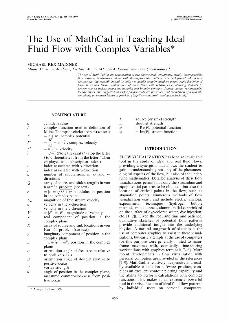
Ffreestream�z� � Uozeÿi� �8�Recalling that � is the real part of the complexfunction, and that is the imaginary part, wehave �i,j = Re(Ffreestream(zi,j)) and i,j =Im (Ffreestream(zi,j)). In the lesson plan, items suchas � and Uo are included in the text as `mathregions' so that they may be varied as desired. Infact, the student is encouraged to do so, and toexamine changes in the output ± this is the realbenefit of a program such as MathCad. As aconsequence of the Cauchy-Riemann equations,the streamlines and equipotential lines are ortho-gonal for all potential flows and for all linearcombinations of these flows. MathCad allowsvarious modifications to the contour plots, includ-ing colors or shades of gray between successivecontours, automatic contour plotting, choice ofnumbers of contours, etc. Figure 1 depicts theequipotential lines and streamlines for a freestream of magnitude Uo = 1 and � � �=3.

Source/SinkThe complex potential for a source is given as:

Fsource�z� � �

2�ln�zÿ zsource� �9�

M. Maixner458

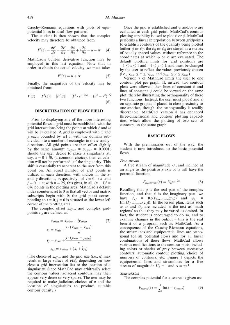
A sink is merely a source of negative strength. InFig. 2 the equipotential lines and streamlines areplotted for a source of strength of � = 2� andlocated at zsource = 0, using the relations i,j =Im(Fsource(zi,j)) and �i,j = Re(Fsource(zi,j)). Noticethat the streamlines all emanate from the originof the source, and that the equipotential lines andstreamlines are everywhere perpendicular. Notealso the concentrations of the streamlines alongthe negative x-axis ± this is the location (withinMathCad) of the so-called Riemann cut; the valueof jumps by a value of 2� as the Riemann cut istraversed.

DoubletA doublet is formed when a source and sink of

equal magnitude are brought together, maintain-ing the product of strength and separation at aconstant value. In the limit, as the separationbetween the source and sink tends towards zero,a doublet of strength � will result with an orienta-

tion relative to the positive x-axis of angle � (fluidemanating from the doublet on the side originallyoccupied by the source, and fluid entering thedoublet on the side originally occupied by thesink); the complex potential is given as:

Fdoublet�z� � ÿ�eÿi�

2��zÿ zdoublet� �10�

Equipotential lines and streamlines for a doublet atthe origin and with strength � = 2� and orientation� = � are depicted in Fig. 3.

VortexFor a vortex of strength ÿ (a positive value of ÿ

results in a counter-clockwise velocity), thecomplex potential is:

Fvortex�z� � ÿiÿ

2�ln�zÿ zvortex� �11�

Fig. 1. Equipotentials and streamlines for free stream of strength U0 � 1 and � � �=3. Note the orthogonality of the two plots.

Fig. 2. Equipotentials and streamlines for source of strength � � 2�.


Figure 4 depicts the equipotentials and streamlinesfor a vortex of strength ÿ = 2� situated at theorigin. At this point, students are shown how theequipotentials for a source are analogous to thestreamlines for a vortex, and vice-versa; this is dueto the fact that their complex potentials are similar,differing only by a factor of ÿi.

COMBINATIONS OF BASIC FLOWS

`Bathtub' vortexBy combining a sink and a vortex, the following

complex potential results:

Fbathtub�z� � ÿ �

2�ln�zÿ zsink� ÿ iÿ

2�ln�zÿ zvortex�

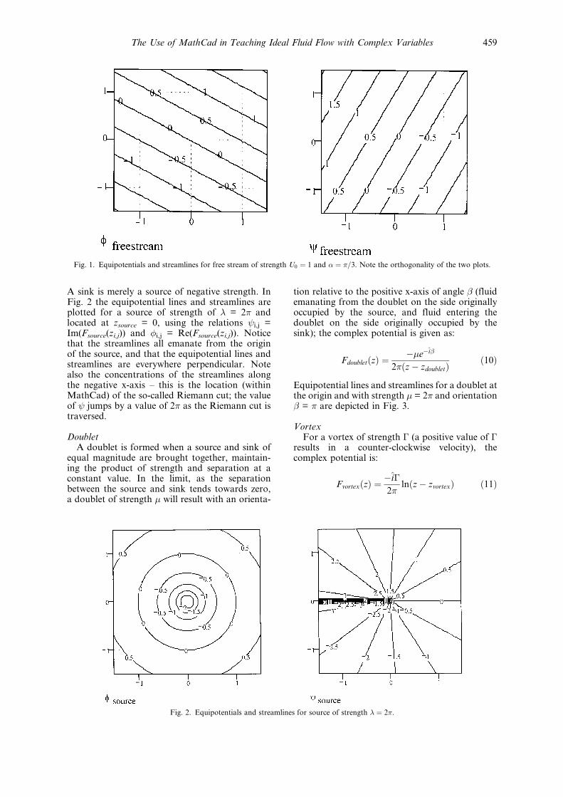
�12�Choosing � = ÿ = 2� and zsink = zvortex = 0, a plotof the streamlines for this flow (Fig. 5) shows thatthe streamlines spiral, with the flow directed

toward the origin. Were a source used instead ofa sink, the flow would spiral outward from theorigin, much as is obtained in a centrifugal pump.

Aircraft trailing vortex systemWhen two vortices of equal magnitude, opposite

sign, and located at z1 and z2 are combined, thefollowing complex potential results:

FTV �z� �ÿiÿ

2��ln�zÿ z1� ÿ ln�zÿ z2�� 13�

�ÿiÿ

2�ln

zÿ z1

zÿ z2

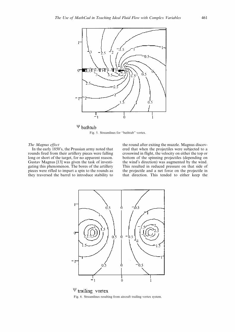
� �Figure 6 depicts the streamlines obtained from twosuch vortices of magnitude 2� and situated z = �1.In fact, what this situation represents is the flowpattern exhibited by a lifting wing, with a trailingvortex emanating from each wingtip. The vorticesare `images' of one another, and result in a plane ofsymmetry at mid-span (x = 0), where = 0.

Fig. 3. Equipotentials and streamlines for a doublet of strength � � 2� and orientation � � �.

Fig. 4. Equipotentials and streamlines for vortex of strength ÿ � 2�.

M. Maixner460

The Magnus effectIn the early 1850's, the Prussian army noted that

rounds fired from their artillery pieces were fallinglong or short of the target, for no apparent reason.Gustav Magnus [13] was given the task of investi-gating this phenomenon. The bores of the artillerypieces were rifled to impart a spin to the rounds asthey traversed the barrel to introduce stability to

the round after exiting the muzzle. Magnus discov-ered that when the projectiles were subjected to acrosswind in flight, the velocity on either the top orbottom of the spinning projectiles (depending onthe wind's direction) was augmented by the wind.This resulted in reduced pressure on that side ofthe projectile and a net force on the projectile inthat direction. This tended to either keep the

Fig. 5. Streamlines for ``bathtub'' vortex.

Fig. 6. Streamlines resulting from aircraft trailing vortex system.


projectile aloft for a longer time (low pressureregion on top) or a shorter time (low pressureregion on the bottom). It is this same phenomenonwhich causes golf balls, baseballs, and other spin-ning spherical objects to deflect in flight [14]. (Seethe article by Swanson [15] for a more recentdiscussion of this effect.) The power of complexvariables may be used to depict this region ofhigher velocity for the two-dimensional, ratherthan the three-dimensional case (i.e., the Magnusproblem of a spinning cylinder, rather than aspinning sphere). This particular problem may beeasily handled with MathCad.

Consider the combination of a freestream ofmagnitude Uo = 1 oriented � = 0 (flow in thepositive x-direction) and a doublet of strength2�Uo oriented � = � (in the negative x-direction)and situated at the origin. This results in a cylinderof unit radius whose surface is the locus of pointswhere = 0. Since there can be no flow throughthe surface of the cylinder (i.e. no normal velocityon the cylinder), the tangential velocity is the totalvelocity along this surface. We will also include avortex of strength ÿ at the origin ± this will later bevaried to investigate the effect of circulation onthe flow pattern. The complex potential thatresults is:

FMagnus�z� � Uoeÿi�zÿ �eÿi�

2�zÿ iÿ

2�ln z �14�

With ÿ = 0, the resulting streamline plot is shownin Fig. 7(a); stagnation points exist on the cylinderat the intersection of the cylinder surface with thex-axis. As the vortex circulation is increased toÿ � ÿ2� (i.e. circulation in a clockwise direction),the stagnation points move to locations on thelower two quadrants of the cylinder, as seen in Fig.7(b). Further increasing the circulation to ÿ � ÿ4�results in the stagnation points meeting at thebottom of the cylinder, Fig. 7(c), and a furtherincrease results in one stagnation point movinginto the flow, and the other moving inside thecylinder, Fig. 7(d)!

The region of more densely packed streamlineson the upper surface of the cylinder corresponds toa region of higher velocity since the free streamvelocity adds to the rotational velocity imparted bythe spinning cylinder. From Bernoulli's theorem,this is also a region of lower pressure, so that a netforce in the positive y-direction results. At thispoint, a discussion of viscous effects and separ-ation is appropriate, since the real flow wouldseparate from the cylinder somewhere in the firstquadrant (i.e. on the downstream side of the uppersurface). It is also instructive to plot the velocity onthe surface of the cylinder at several points for theideal (i.e. unseparated) flow. A device employingthis principle (a 26-meter high `turbosail') will beinstalled as a means of supplementing moreconventional means of propulsion on Calypso II,the research vessel for the Cousteau Society ± it isanticipated that fuel savings on the order of 30 per

cent will be realized when compared to the fuelconsumption of a more conventional vessel of thesame size [16].

PROBLEMS FOR FURTHER STUDY

The basic flows and combinations thereof arecontained in the lesson plan posted on the Math-Cad web site; the following constitute additionalproblems which may be employed as homeworks,projects, or to merely spark discussion.

Wing in ground effectAs an extension of the lifting wing problem,

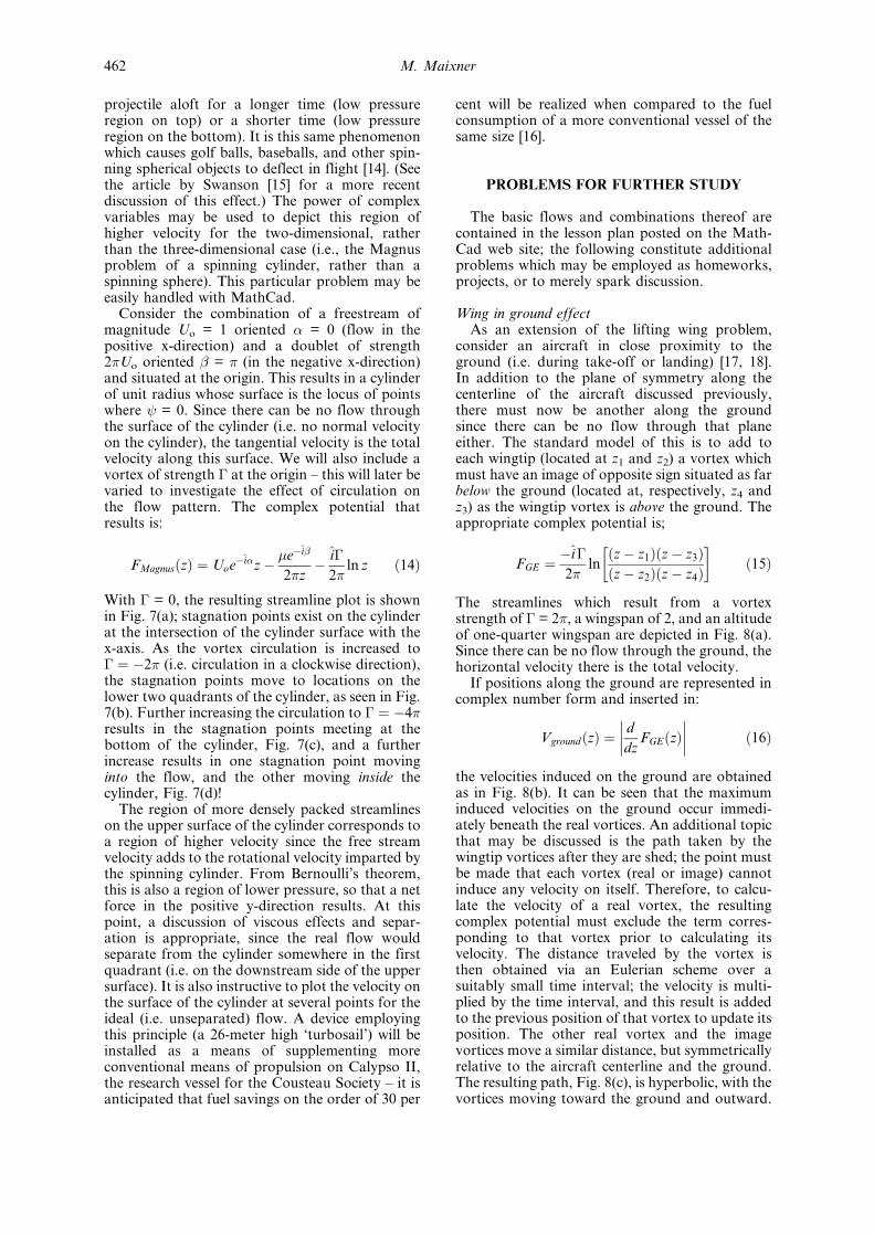
consider an aircraft in close proximity to theground (i.e. during take-off or landing) [17, 18].In addition to the plane of symmetry along thecenterline of the aircraft discussed previously,there must now be another along the groundsince there can be no flow through that planeeither. The standard model of this is to add toeach wingtip (located at z1 and z2) a vortex whichmust have an image of opposite sign situated as farbelow the ground (located at, respectively, z4 andz3) as the wingtip vortex is above the ground. Theappropriate complex potential is;

FGE � ÿiÿ

2�ln�zÿ z1��zÿ z3��zÿ z2��zÿ z4��

�15�

The streamlines which result from a vortexstrength of ÿ = 2�, a wingspan of 2, and an altitudeof one-quarter wingspan are depicted in Fig. 8(a).Since there can be no flow through the ground, thehorizontal velocity there is the total velocity.

If positions along the ground are represented incomplex number form and inserted in:

Vground�z� � d

dzFGE�z�

�� 16�

the velocities induced on the ground are obtainedas in Fig. 8(b). It can be seen that the maximuminduced velocities on the ground occur immedi-ately beneath the real vortices. An additional topicthat may be discussed is the path taken by thewingtip vortices after they are shed; the point mustbe made that each vortex (real or image) cannotinduce any velocity on itself. Therefore, to calcu-late the velocity of a real vortex, the resultingcomplex potential must exclude the term corres-ponding to that vortex prior to calculating itsvelocity. The distance traveled by the vortex isthen obtained via an Eulerian scheme over asuitably small time interval; the velocity is multi-plied by the time interval, and this result is addedto the previous position of that vortex to update itsposition. The other real vortex and the imagevortices move a similar distance, but symmetricallyrelative to the aircraft centerline and the ground.The resulting path, Fig. 8(c), is hyperbolic, with thevortices moving toward the ground and outward.

M. Maixner462

At this point, a discussion is appropriate of theeffect that the trailing vortices shed by a largeaircraft could have on smaller aircraft, and whythere can be a significant wait on the ground asaircraft queue for take-off.

Von KaÂrmaÂn problemIn the 1920s, Theodore von KaÂrmaÂn was

contracted by the Zeppelin company to investigatethe pressure distributions on airship hulls. Hisingenious method of combining various singula-rities to obtain the required airship body profiles,although created for the axisymmetric case, maybe easily demonstrated with MathCad using com-binations of the two-dimensional singularities

discussed above. For a detailed discussion of themethod, see References [19±22].

Von KaÂrmaÂn's method begins by placing a seriesof sources towards the bow along the centerline(i.e. the x-axis) of the body, and a series of sinks onthe centerline towards the stern. The body ispresumed to be operating head-on into a freestream of magnitude Uo. The sum of all sourcesshould equal the sum of all sinks, so that there willnot be any flow through the body. What isrequired is the proper combination of source andsink strengths and locations so that the body'soutline is matched by the = 0 streamline.

A drawback of MathCad (before version 8) isthat no other plot may be superposed on a contour

Fig. 7. Streamlines for flow about a cylinder with: (a) No circulation, with two stagnation points situated on x-axis; (b) Circulation ofintermediate strength ÿ � ÿ2�, with two stagnation points moving down and towards each other; (c) Critical circulation of ÿ � ÿ4�,resulting in one stagnation point at the bottom of the cylinder; (d) Circulation of strength ÿ � ÿ4:03�, with one stagnation point

moving towards the origin (inside cylinder) and the other in the flow moving away from the cylinder.


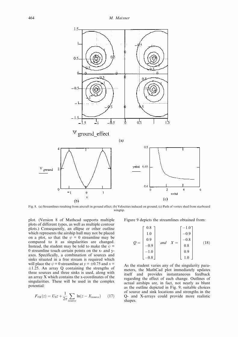
plot. (Version 8 of Mathcad supports multipleplots of different types, as well as multiple contourplots.) Consequently, an ellipse or other outlinewhich represents the airship hull may not be placedon a plot, so that the = 0 streamline may becompared to it as singularities are changed.Instead, the student may be told to make the =0 streamline touch certain points on the x- and y-axes. Specifically, a combination of sources andsinks situated in a free stream is required whichwill place the = 0 streamline at y =�0.75 and x =�1.25. An array Q containing the strengths ofthree sources and three sinks is used, along withan array X which contains the x-coordinates of thesingularities. These will be used in the complexpotential:

FVK�z� � U0z� 1

2�

Xisource

ln�zÿ Xisource� �17�

Figure 9 depicts the streamlines obtained from:

Q �

0:8

1:0

0:9

ÿ0:9

ÿ1:0

ÿ0:8

2666666664

3777777775and X �

ÿ1:0

ÿ0:9

ÿ0:8

0:8

0:9

1:0

2666666664

3777777775�18�

As the student varies any of the singularity para-meters, the MathCad plot immediately updatesitself and provides instantaneous feedbackregarding the effect of each change. Outlines ofactual airships are, in fact, not nearly as bluntas the outline depicted in Fig. 9; suitable choicesof source and sink locations and strengths in theQ- and X-arrays could provide more realisticshapes.

Fig. 8. (a) Streamlines resulting from aircraft in ground effect; (b) Velocities induced on ground; (c) Path of vortex shed from starboardwingtip.

M. Maixner464

Circle theoremWith the aircraft trailing vortex example, the

aircraft centerline was seen to be a plane throughwhich no flow passed; similarly, an aircraft inground effect also had no flow through the planethat represented the ground. This technique isreferred to as the method of images, and is notrestricted to plane boundaries. In fact, Milne-Thompson's circle theorem [23] states that if thecomplex potential f(z) represents a flow withoutsingularities for |z| < a, then:

F�z� � f �z� � �fa2

z

� ��19�

represents the same flow at infinity with a circle ofradius `a' at the origin. (When used on a function,the overbar notation �f indicates that all complexconstants in the original function f are now theircomplex conjugates.) In the case of a vortex situatedat zreal in the vicinity of a circular cylinder of unitradius, the circle theorem gives the complex potential:

F�z� � ÿiÿ

2�ln�zÿ zreal� � iÿ

2�ln

1

zÿ �zreal

� ��20�

Following a bit of algebra, this equation may berecast as:

F�z� �ÿiÿ

2�ln�zÿ zreal� � iÿ

2�ln zÿ 1

�zreal

� �ÿ iÿ

2�ln z� iÿ

2�ln�ÿ�zreal� �21�

Studying the right hand side of this last equationreveals that the first term is the real vortex; thesecond term is an image vortex of equal (butopposite) strength situated at 1=�zreal ; the thirdterm is a vortex of the same magnitude and senseas the real vortex, but located at the origin; thelast term is a constant which ensures that thelocus of = 0 coincides with |z| = a = 1. Hadthe last term been left off, there would still be acircular streamline on |z| = a = 1, but itsvalue would be non-zero. It is a simple matterto plot the resulting streamlines using either ofthe last two equations in MathCad; additionally,if the second equation is used, the change instreamline values which occurs when the lastterm is included or left out can be readily andquickly observed.

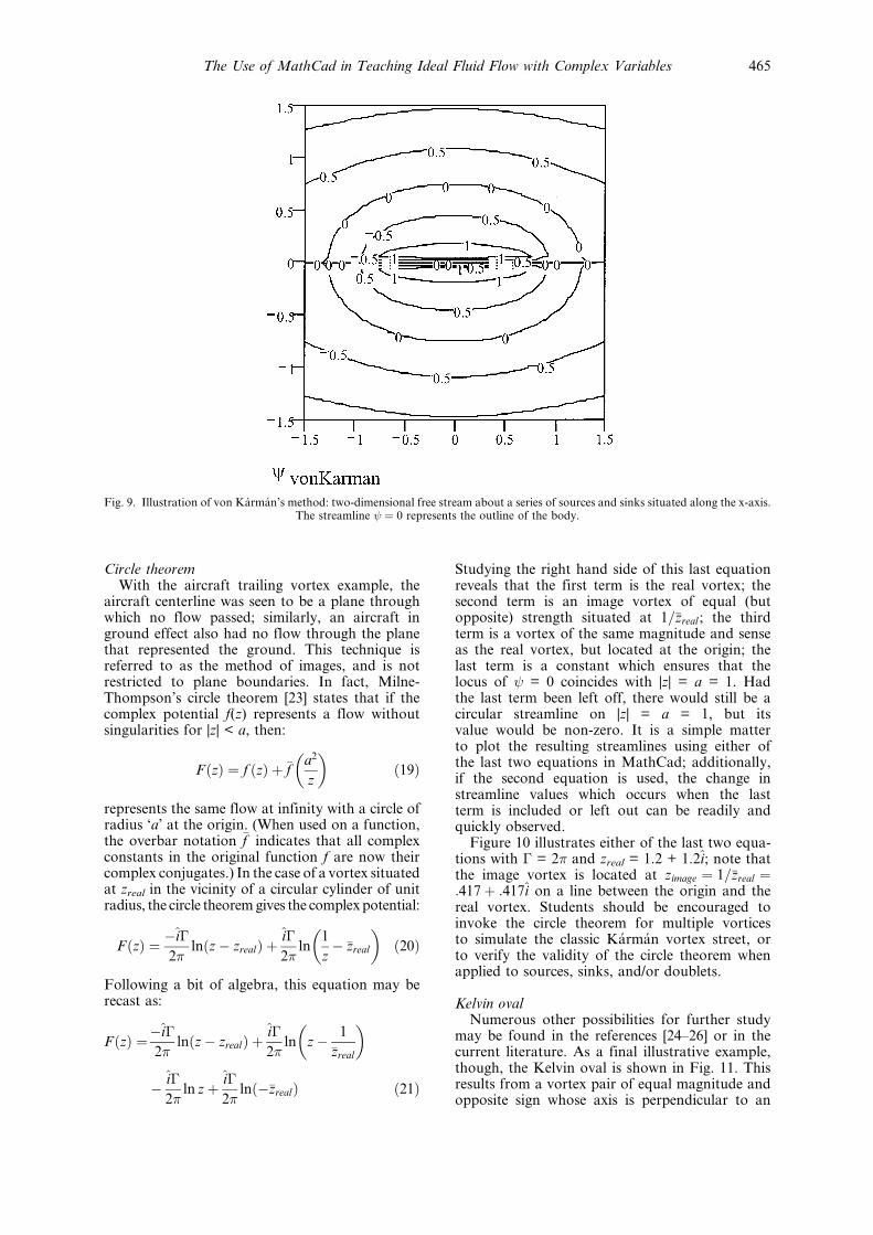
Figure 10 illustrates either of the last two equa-tions with ÿ = 2� and zreal = 1.2 + 1.2i; note thatthe image vortex is located at zimage � 1=�zreal �:417� :417i on a line between the origin and thereal vortex. Students should be encouraged toinvoke the circle theorem for multiple vorticesto simulate the classic KaÂrmaÂn vortex street, orto verify the validity of the circle theorem whenapplied to sources, sinks, and/or doublets.

Kelvin ovalNumerous other possibilities for further study

may be found in the references [24±26] or in thecurrent literature. As a final illustrative example,though, the Kelvin oval is shown in Fig. 11. Thisresults from a vortex pair of equal magnitude andopposite sign whose axis is perpendicular to an

Fig. 9. Illustration of von KaÂrmaÂn's method: two-dimensional free stream about a series of sources and sinks situated along the x-axis.The streamline � 0 represents the outline of the body.


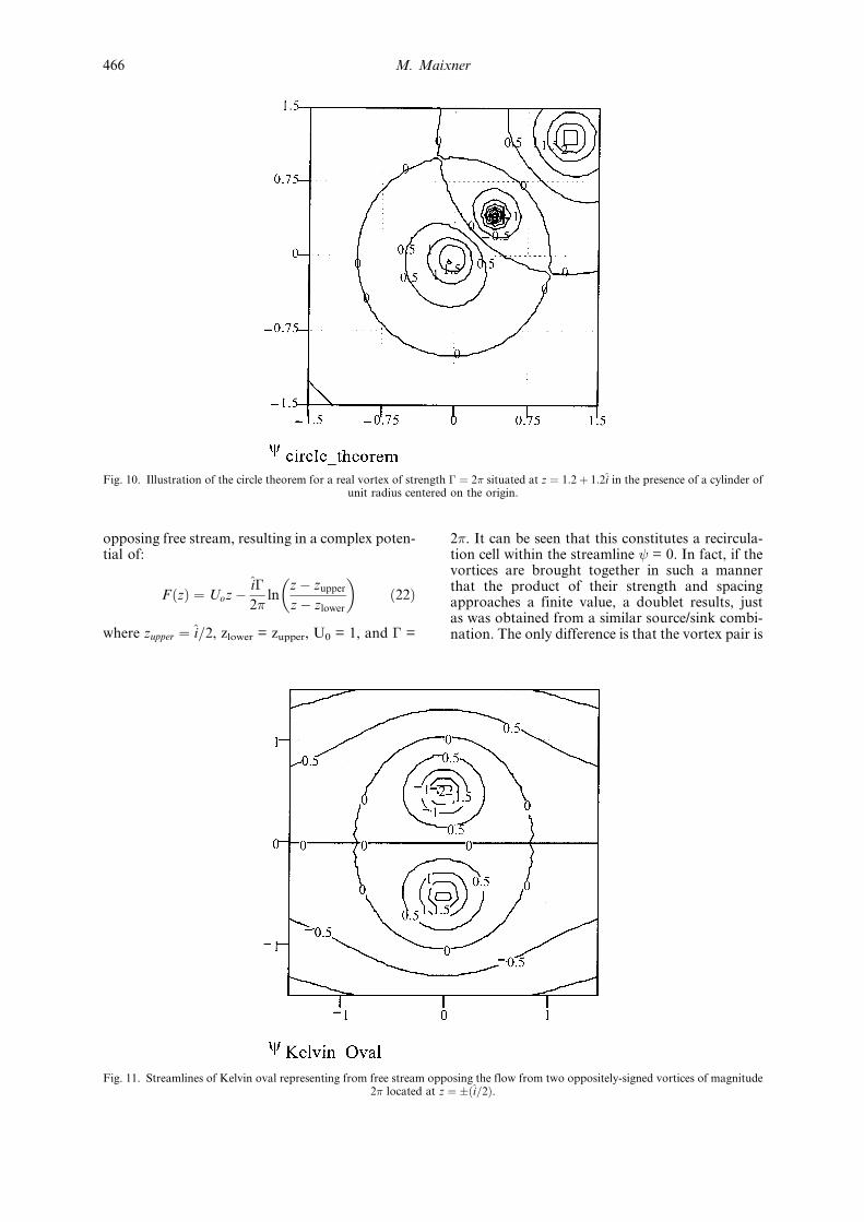
opposing free stream, resulting in a complex poten-tial of:

F�z� � Uozÿ iÿ

2�ln

zÿ zupper

zÿ zlower

� ��22�

where zupper � i=2, zlower = zupper, U0 = 1, and ÿ =

2�. It can be seen that this constitutes a recircula-tion cell within the streamline = 0. In fact, if thevortices are brought together in such a mannerthat the product of their strength and spacingapproaches a finite value, a doublet results, justas was obtained from a similar source/sink combi-nation. The only difference is that the vortex pair is

Fig. 11. Streamlines of Kelvin oval representing from free stream opposing the flow from two oppositely-signed vortices of magnitude2� located at z � ��i=2�.

Fig. 10. Illustration of the circle theorem for a real vortex of strength ÿ � 2� situated at z � 1:2� 1:2i in the presence of a cylinder ofunit radius centered on the origin.

M. Maixner466

oriented perpendicular to the free stream, while thesource/sink combination lies on an axis parallel tothe free stream.

CONCLUSION

MathCad is an inexpensive and readily availablecalculation software package which, even in thestudent version, contains a powerful contour plot-ting routine and the ability to perform calculationswith complex numbers. These features make it an

excellent choice for teaching ideal fluid flow withcomplex variables. The lesson plan provided on theMathCad web site may be easily modified to suitindividual teaching preferences or topics. Withminimal effort, the lesson plan may be changedto provide instruction in electrostatics. The streamfunction for the fluid flow problem is analogousto the potential function in the electrostatic analog;likewise, the potential function � (and the equipo-tentials) of the fluid flow problem find theirparallels in the stream function (and lines offorce) of electrostatics.

REFERENCES

1. G. J. Hokensen and R. D. W. Bowersox, Flow visualization, in Handbook of Fluid Dynamics andFluid Machinery, Volume II: Experimental and Computational Fluid Dynamics, ed. J. A. Schetz andA. E. Fuhs, Wiley, New York, (1996) pp. 1019 ±1039.

2. B. Carr and V. E. Young, Videotapes and movies on fluid dynamics and fluid machines, inHandbook of Fluid Dynamics and Fluid Machinery, Volume II: Experimental and Computa-tional Fluid Dynamics, ed. J. A. Schetz and A. E. Fuhs, Wiley, New York, (1996) pp. 1171±1189.

3. J. C. Bruch, Jr. and R. C. Wood, The teaching of hydrodynamics using computer generateddisplays, Bull. Mech. Engng. Educ., 9, (1970) pp. 105±115.

4. D. R. Broome, Interactive graphics display of inviscid fluid flows developed using conformaltransformations, IJMEE, 6 (4), (1978) pp.191±195.

5. J. C. Bruch, Jr., The use of interactive computer graphics in the conformal mapping area,Computers & Graphics, 1, (1975) pp. 361±374.

6. R. C. Wood and J. C. Bruch, Jr., Teaching complex variables with an interactive computer system,IEEE Transactions on Education, V-15 (1), (Feb 1972) pp. 73±80.

7. J. Mittleman and A. K. Mitra, Exploring two-dimensional potential flow on a personal computer,Computers in Education Journal, IV (1), (Jan±Mar 1994) pp. 70±76.

8. T. A. Fenaish, Numerical experiments on potential flow configurations, Computers in EducationJournal, II (4), (Oct±Dec 1992) pp. 17±20.

9. R. C. Ertekin and B. Padmanabhan, Graphical aid in potential flow problems: computer programPOTFLO, Computers in Education Journal, IV (4), (Oct±Dec 1994) pp. 24±31.

10. F. B. Hildebrand, Advanced Calculus for Applications, Prentice-Hall, Englewood Cliffs NJ (1962)Ch. 10.

11. E. Kreyszig, Advanced Engineering Mathematics, 8th ed., Wiley, New York (1999) Ch. 12.12. V. L. Streeter, E. B. Wylie and L. W. Bedford, Fluid Mechanics, 9th ed., WCB/McGraw-Hill,

Boston (1998) Ch. 8.13. G. Magnus, UÈ ber die Abweichung von Geschossen [On the deviation of shots (projectiles)], Abh.

Der Berlin Akad, 1851; UÈ ber die Abweichung der Geschosse und Auffallende Erscheinungen beiRotierenden KoÈrpern, Ann. Phys., 88, 1853, p. 1.

14. J. W. Strutt, Lord Rayleigh, On the irregular flight of a tennis ball, Messenger of Math., 7 (1877);Scientific Papers, 1, pp. 344±46.

15. W. M. Swanson, The Magnus effect: a summary of investigations to date, Journal of BasicEngineering, Trans. Am. Soc. Mech. Eng., 83D, (September 1961) pp. 461±470.

16. The Cousteau Society, Calypso IIÐA Revolutionary, Environmentally Friendly Ship, web site http://www.pilot.infi.net/ ~merriam/cousteau/page/calyp2.htm (March 10, 1999).

17. J. K. Harvery and F. J. Perry, Flowfield produced by trailing vortices in the vicinity of the ground,AIAA Journal, 9, (8), (1971) pp. 1659±60.

18. Z. C. Zheng and R. L. Ash, Study of aircraft wake vortex behavior near the ground, AIAA Journal,34 (3), (March 1996) pp. 580±589.

19. T. von KaÂrmaÂn, Berechnung der Druckverteilung an LuftschiffkoÈrpoÂrn, Abhandlungen aus demAerodynamischen Institut an der Technischen Hochschule Aachen, 6, (1927) pp. 3±17. Translatedas NACA TM 574: Calculation of Pressure Distribution on Airship Hulls, by M. Miner (July1930).

20. J. M. Robertson, Hydrodynamics in Theory and Application, Prentice-Hall, Englewood Cliffs NJ(1965).

21. C. Y. Chow, An Introduction to Computational Fluid Mechanics, John Wiley & Sons, New York(1979) Ch. 2.

22. J. L. Hess, Potential Flow, in Handbook of Fluid Dynamics and Fluid Machinery, Volume I:Fundamentals of Fluid Dynamics, ed. J. A. Schetz and A. E. Fuhs, Wiley, New York, (1996)pp. 55±56.

23. L. M. Milne-Thompson, Theoretical Hydrodynamics, 5th ed., MacMillan, London (1968).24. H. R. Vallentine, Applied Hydrodynamics, Butterworths, London (1969).25. J. Katz and A. Plotkin, Low-Speed Aerodynamics: From Wing Theory to Panel Methods, McGraw-

Hill, New York (1991).26. H. Glauert, The Elements of Aerofoil and Airscrew Theory, 2nd ed., Cambridge University Press,

Cambridge (1947).


Michael Rex Maixner graduated with distinction from the United States Naval Academy(1972), and served as a commissioned officer in the United States Navy for 25 years; his first12 years were spent as a line (shipboard) officer, while his remaining service was spentstrictly in engineering assignments. He received his Ocean Engineer and SMME degreesfrom MIT (1977), and his Ph.D. in mechanical engineering from the Naval PostgraduateSchool (1994). His military service included 2 years on the faculty at the Naval Post-graduate School. Upon completing his military service in 1997, he accepted a position asAssociate Professor of Engineering at Maine Maritime Academy in Castine, Maine.

M. Maixner468

potential flows

Documents