arX

iv:m

ath/

0305

307v

2 [

mat

h.O

C]

25

Nov

200

3

Positive forward rates in the maximum smoothness

framework

Julian Manzano∗

Division of Applied Physics.

Institute of Physics and Measurement Technology.

Linkoping University.

and

Jorgen Blomvall

Division of Optimization. Department of Mathematics.

Linkoping University.

Abstract

In this article we present a non-linear dynamic programming algorithm for the com-

putation of forward rates within the maximum smoothness framework. The algorithm

implements the forward rate positivity constraint for a one-parametric family of smooth-

ness measures and it handles price spreads in the constraining dataset. We investigate the

outcome of the algorithm using the Swedish Bond market showing examples where the

absence of the positive constraint leads to negative interest rates. Furthermore we inves-

tigate the predictive accuracy of the algorithm as we move along the family of smoothness

measures. Among other things we observe that the inclusion of spreads not only improves

the smoothness of forward curves but also significantly reduces the predictive error.

May 2003

∗corresponding author: Julian Manzano, Division of Applied Physics. Institute of Physics and Measure-

ment Technology. Linkoping University, S-581 83 Linkoping, Sweden; e-mail: manzano@ifm.liu.se; phone:

+46.737.353.373.

1

1 Introduction

Within the financial industry forward rate curves play a central role in fixed-income derivative

pricing and risk management. Notwithstanding, such curves are not empirical or directly

measurable objects but rather useful abstract concepts from where observed prices can be

derived. Moreover, given a finite set of market prices, we can construct in general an infinite

number of compatible forward rate curves1. To avoid such ambiguity several approaches have

been proposed in the literature trying to capture a “reasonable” or “natural” functional form

within the set of compatible possibilities.

In historical order the first kind of methods proposed to solve this problem make use

of the so-called parametric approach. In this approach a particular functional form for the

forward rate curve is assumed leaving a certain number of free parameters to be fixed from

the calculation of a given set of quoted prices. An extensive literature exists advocating for

this approach. We can cite as examples the works of McCulloc [1], Vasicek and Fong [2],

Chambers, Carleton and Waldman [3], Shea [4], Nelson and Siegel [5] and more recently the

works of Svensson [6], Fisher, Nychka and Zervos [7] and Waggoner [8]. In most of these works

we notice the privileged role played by polynomial and exponential splines as the preferred

functional forms for the forward rate curves.

The second kind of methods has been termed in the literature as non-parametric or

maximum-smoothness approach. Here instead of advocating for an a priori functional form

for the forward rate a given measure of smoothness is chosen and then the forward rate curve

is obtained as the one maximizing this measure subject to the constraints imposed by market

prices. Examples where these methods have been investigated include the works of Adams

and Van Deventer [9], Delbaen and Lorimier [10], Kian Guan Lim, Qin Xiao et al [11, 12],

Frishling and Yamamura [13] and Yekutieli [14]. In these works three different smoothing

measures have been proposed. We also have the works of Forsgren [15] and Kwon [16]

that generalize these methodologies and clarify the connection between splines and certain

smoothness measures. Finally we point out the work of Wets, Bianchi and Yang [17] that

can be located somewhere in-between both approaches since here the number of functional

parameters is finite (albeit arbitrarily large) and the functional behavior is restricted to a

subfamily of C2 curves.

The purpose of this article is two-fold: Firstly we want to present an efficient maximum-

smoothing algorithm that handles the presence of spreads and implements the positivity

constraint. Secondly we want to investigate the predictive power of a linear combination

of two quadratic measures, namely the one proposed by Delbaen et al. and Frishling et al.

1We assume here that prices do not allow for arbitrage. If this is not the case the compatibility condition

has to be relaxed.

2

[10, 13] and the one by Adams and van Deventer [9]. Here it is worth remarking that once

the compatibility with market prices is fulfilled the only guiding principle that should be

taken as definition of “reasonable” or “natural” is the predictive power and not other ad-hoc

criteria.

In this article we will only use as constraining data coupon bearing bonds. The inclusion

of treasury bills, zero coupon bonds or bill futures is straightforward and amounts to adding

the corresponding linear constraints. Since our objective in this article is focusing on an algo-

rithm dealing with non-linear constraints and inequality constraints (spreads and positivity

constraint) we have not included such data.

With these objectives in mind we organize the article as follows:

In section 2 we present the objective function that we will use throughout the article

and we establish the basic notation. In this section we present a sketch of the complete

algorithm leaving the details for the appendices. In section 3 we present the results of the

article including examples where the absence of the positivity constraint or the adequate

spreads leads to negative rates. Here we present also a study of the predictive power of the

one-parametric family of smoothness measures that include as extreme cases the measures

used by Delbaen et al., Frishling et al. and Adams and Van Deventer. Finally in section 4

we present the conclusions.

2 The algorithm

A bond, j, is an instrument that gives future coupons, cij , at time stages R(j)i , i = 1, . . . , nj−1

and a final payment, cnjj = Nj2. The bond price, Pj , can be determined from the discrete

forward rate curve, fr, r = 1, . . . , R(j)nj

, as follows

Pj =

nj∑

i=1

cij exp

−

R(j)i

−1∑

r=1

frξr

, (1)

where ξr is the length of the time period between time stage r and r+1 (in our implementation

we have used ξr = 1 day).

The objective function, or smoothing measure3, is defined as a linear combination of the

one used by Delbaen et al. and Frishling et al. (DF) [10, 13] and the one used by Adams and

2By final payment Nj we mean the complete last cash flow of bond j, typically that includes a principal

plus a last coupon.3Note that since we do not include a global minus sign we have to perform a minimization and not a

maximization. With this sign, that is the one used in the literature, “rugosity” measure would be a more

appropriate name.

3

Van Deventer (AD) [9]

W :=γ

2

n−1∑

r=1

(

fr+1 − frξr

)2

ξr +ϕ

2

n−1∑

r=2

(

2

(ξr−1 + ξr)

(

fr+1 − frξr

−fr − fr−1

ξr−1

))2

ξr, (2)

The first term in Eq.(2) (DF) is a discrete approximation of the integral of the square of the

first derivative of f and the second term (AD) is a discrete approximation of the integral of

the square of the second derivative of f . This objective function is to be minimized subject

to the consistency constraints

0 = ρj +

R(j)nj

−1∑

r=1

frξr − ln (vj) , (3)

fr ≥ 0, ρbj ≤ ρj ≤ ρaj , (4)

where ρj = ln (Pj/Nj) is to be determined along with f and where we have used the definitions

vj :=

nj∑

i=1

αij exp

R(j)nj

−1∑

r=R(j)i

frξr

, ρbj := ln

(

αb0j

)

, ρaj := ln(

αa0j

)

,

αij :=cijNj

, αb0j :=

P bj

Nj, αa

0j :=P aj

Njαnjj := 1, (5)

with P bj , P

aj the respective bid and ask prices of bond j (j = 1, · · · ,m)4. Note that the

equality constraint given by Eq.(3) is just Eq.(1) rewritten taking logarithms and using the

definitions (5). Eq.(4) introduces two inequality constraints. The first one is the positivity

constraint over the forward rate curve and the second one is the requirement that the single

price given by Eq.(1) must lie in-between the bid and ask prices.

We define the spread of bond j as the quantity ρaj − ρbj. We take the largest time to

maturity in Eq.(2) equal to the largest time to maturity in the constraining dataset, namely

n := maxj

(

R(j)nj

)

.

The constraints reflecting bond prices (1) have been rewritten in a way such that they

become linear when no coupons are present (vj = 1 for a zero–coupon bond j). Constraints

given by Eqs.(3) and (4) are moved to the objective function defining

Z := W+m∑

j=1

λj

ρj +

R(j)nj

−1∑

r=1

frξr − ln (vj)

−µ

n∑

r=1

ln (fr)−µm∑

j=1

(

ln(

ρj − ρbj

)

+ ln(

ρaj − ρj)

)

,

(6)

4Note that this optimization problem is non-convex and therefore several local minima may exist.

4

with the Lagrange multipliers λj, j = 1, . . . ,m and the logarithmic barriers with parameters

µ > 0 and µ > 0 (in the solution procedure we take µ → 0, µ → 0). The use of log barriers

to deal with inequality constraints is a standard methodology in interior point methods for

optimization problems [18]. An explanation of this methodology adapted to our problem is

given in appendix A. Briefly the minimization algorithm is structured as follows:

step 0: Initialize log barriers with coefficients µ[0], µ[0] and set (f, ρ) = (f [0], ρ[0])

with the seed (f [0], ρ[0]) satisfying the inequality constraints (4). Let k = 0.

step 1: Make a second order approximation of Z at (f [k], ρ[k]) (see appendix A).

step 2: Determine the newton step (f [k+1], ρ[k+1]) using dynamic programming (see appendix B).

step 3: Modify (f [k+1], ρ[k+1]) to get a solution (f [k+1], ρ[k+1]) that satisfies the inequality

constraints (4). Update log barriers (µ[k] → 0 and µ[k] → 0 as k → ∞) and

calculate the values of W and of constraints (3). Check if a termination criterion

is satisfied, otherwise let k = k + 1 and go to step 1 (see appendix C). (7)

Computing times involved in step 2 are summarized in subsection B.1. The solution typically

stabilizes in approximately 6 iterations as can be seen in Fig.(1). On a Pentium 4, 2.4 Ghz

computer the algorithm coded in C++ takes around 1/4 sec. to compute a forward rate

curve like any of the ones seen in Fig.(2).

3 Consistency and predictability

In this section we present some examples of the behavior of algorithm (7) and we investigate

the predictive power of the resulting forward rate curves. In Fig.(2) we present a series of

forward rate curves calculated using DF and AD smoothing measures. There we can see

that for both measures the resulting curves share some similar traits like the positions of

most peaks and dips. Clear differences between both sets of curves are found at their end-

points and in their behavior in the presence of high spreads. In the set of curves obtained

from the DF measure we have vanishing first derivative at the end-points and curves that

tend to constants for high spreads. For the AD measure we have vanishing second and third

derivatives at end-points [16] and curves for high enough spreads given by straight lines. From

the financial point of view these features are, in principle, just different aesthetic possibilities.

In order to choose a particular measure the guiding principles should be, in the first place,

the fulfillment of the consistency constraints given by Eqs.(3-4) and after this is guaranteed

the predictive performance.

Let us start now with the analysis of consistency. As can be found in [16] if we do not

5

0 2 4 6 8 10 12 14 16 18 2010-6

10-5

10-4

10-3

10-2

10-1

100

0 2 4 6 8 10 12 14 16 18 2010-11

10-10

10-9

10-8

10-7

10-6

10-5

10-4

10-3

10-2

10-1

100

101

Sweden, July 2001 Friday 06 Monday 09 Tuesday 10 Wednesday 11 Thursday 12 Friday 13 Monday 16 Tuesday 17 Wednesday 18 Thursday 19

Newton iterationsNewton iterations

W

( =

1 y

ear3 ,

= 0

)(b)

W

( =

0,

= 1

yea

r5 )

(a)

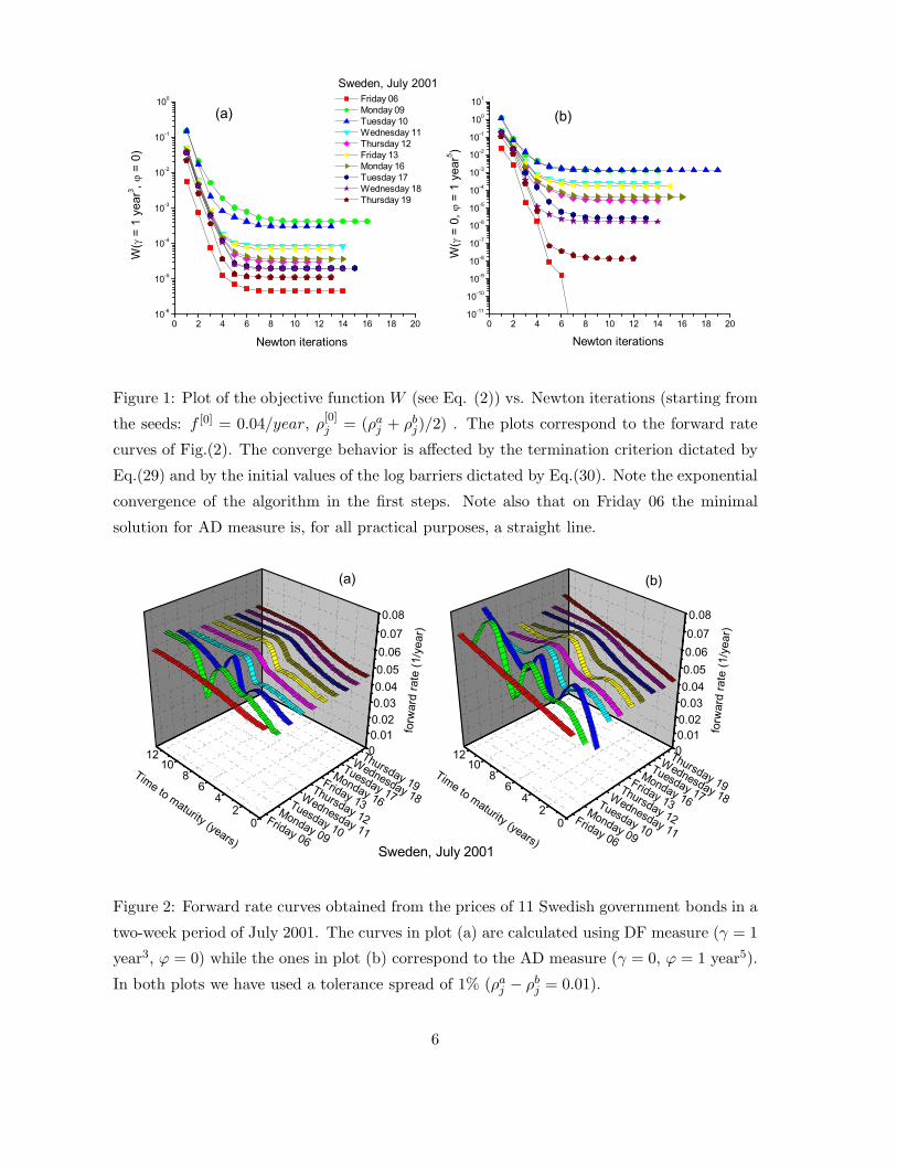
Figure 1: Plot of the objective function W (see Eq. (2)) vs. Newton iterations (starting from

the seeds: f [0] = 0.04/year, ρ[0]j = (ρaj + ρbj)/2) . The plots correspond to the forward rate

curves of Fig.(2). The converge behavior is affected by the termination criterion dictated by

Eq.(29) and by the initial values of the log barriers dictated by Eq.(30). Note the exponential

convergence of the algorithm in the first steps. Note also that on Friday 06 the minimal

solution for AD measure is, for all practical purposes, a straight line.

02

46

810

12 00.010.020.030.040.050.060.070.08

Friday 06

Monday 09

Tuesday 10

Wednesday 11

Thursday 12

Friday 13

Monday 16

Tuesday 17

Wednesday 18

Thursday 19

02

46

810

12 00.010.020.030.040.050.060.070.08

Friday 06

Monday 09

Tuesday 10

Wednesday 11

Thursday 12

Friday 13

Monday 16

Tuesday 17

Wednesday 18

Thursday 19

forw

ard

rate

(1/y

ear)

Time to maturity (years)Sweden, July 2001

(a) (b)

forw

ard

rate

(1/y

ear)

Time to maturity (years)

Figure 2: Forward rate curves obtained from the prices of 11 Swedish government bonds in a

two-week period of July 2001. The curves in plot (a) are calculated using DF measure (γ = 1

year3, ϕ = 0) while the ones in plot (b) correspond to the AD measure (γ = 0, ϕ = 1 year5).

In both plots we have used a tolerance spread of 1% (ρaj − ρbj = 0.01).

6

consider the positivity constraint the local minima of objective (2) are given by exponential

splines with exponents ±√

γ/ϕ or polynomial splines of order 2 or 4 when ϕ or γ are re-

spectively zero. The main problem with these exponential or polynomial splines is that there

is no warranty that they fulfill the positivity constraint. Negative rates are not admissible

in the absence of arbitrage opportunities and the risk of obtaining this unwanted feature

is illustrated in Fig.(3). In this figure we have concentrated on the Swedish bond data on

Monday, July 09, 2001. There we have tested three spread patterns for both DF and AD

measures with and without the positivity constraint. From these plots it is evident that the

inclusion of spreads in the calculation of the forward rates is a necessary ingredient that can

have a major impact in the resulting functional behavior.

Once we have an algorithm that insures the consistency of forward rates we can concen-

trate on the predictive accuracy of different measures. However, before starting the analysis

of this issue let us make a brief digression to comment a point regarding measure (2). If we

want to have both γ and ϕ different from zero and we want to compare the effects of each

term it is important to realize that DF and AD measures scale differently under changes of

time units. In other words, γ and ϕ have different units. A practical way to define their units

is to consider the objective W as an adimensional quantity. By doing so and remembering

that f has units of inverse time, it is immediate to obtain that γ has units of time3 and ϕ

units of time5. The importance of keeping this in mind becomes apparent in results like the

ones presented in Figs.(4) and (5).

Figs.(4) and (5) summarize our results regarding the predictive accuracy of the algorithm

as a function√

γ/ϕ. There it is clear that the characteristic time span where DF and AD

compete is not the day or the century, but clearly the year. To construct these figures

we have calculated the forward rate curves for different values of√

γ/ϕ when one bond is

removed from the constraining dataset. The price of this missing bond is used afterwards

as a benchmark to test the accuracy of the resulting curves. Since we are interested in

the statistical performance we have done such comparison for 335 consecutive trading days

starting on Wednesday, November 08, 2000 and ending on Thursday, March 07, 2002.

We are also interested in studying the impact of spreads in the constraining dataset over

the predictive accuracy. Therefore we present our results for three spread patterns, namely

constant spreads of 0%, 0.5% and 1% in the constraining dataset. Fig.(4) concentrates on the

predictive accuracy for the first 9 bonds of Table (2) and Fig.(5) presents the same analysis

for the remaining 2 bonds of Table (2). These last 2 bonds are the ones with the larger

maturities in the complete dataset. In particular for the last one with the largest maturity

we have to decide upon the methodology to extrapolate the forward curve outside the range

7

of the constraining dataset5. Therefore in Fig.(5) we present the prediction accuracy using

constant extrapolation from the last maturity in the constraining dataset and “W -generated”

extrapolation that consists in utilizing the W -optimal forward rate curve even outside the

range of the constraining dataset.

4 Results and conclusions

In this article we have presented a non-linear dynamic programming algorithm designed for

the calculation of positive definite forward rate curves using data with or without spreads.

We have included multiple details of the algorithm aiming at practitioners not familiar with

the techniques of dynamic programming. We have illustrated the results of this algorithms

using the Swedish bond data for a one-parametric family of smoothness measures.

The results and conclusions are the following:

• The proposed algorithm calculates forward rate curves in real time and admits, with-

out time or complexity penalizations, the use of any non-linear local objective function.

Since it also handles non-linear constraints it is possible to include within the constrain-

ing dataset any derivative products with prices bearing some dependence on forward

rates.

• This is the first algorithm proposed in the literature that implements the positivity

constraint in the maximum smoothness framework. To the knowledge of the authors

the only other work that implements such constraint outside this framework is the one

of Wets et al. [17]. The proposal in [17] has the advantage of using simple linear

programming but do not consider the presence of spreads minimizing instead the sum

over the modulus of the difference between calculated prices and market prices.

• For the objective functions and constraining datasets like the ones we have used or more

generally for the ones studied in [16] the algorithm proposed in that reference offers

better computing times at the expense of ignoring the positivity constraint. Essentially

the complexity in [16] is c3 and in ours is n c2 where n is the number of time steps and

c the number of constraints. For that reason, when this class of objective functions and

constraining datasets are used, a well coded algorithm might try first the proposal in

[16] (improving its treatment of the spreads using e.g. log-barriers) and later, only if

the result is not positive definite, use our approach.

5By the range of the constraining dataset we mean the range in time to maturity that goes from present

to the last maturity within the dataset.

8

2 4 6 8 10 12 14

-0.05

0.00

0.05

0.10

0.15

0.20

2 4 6 8 10 12 14

-0.05

0.00

0.05

0.10

0.15

0.20

2 4 6 8 10 12 14

-0.05

0.00

0.05

0.10

0.15

0.20

2 4 6 8 10 12 14

-0.20

-0.15

-0.10

-0.05

0.00

0.05

0.10

0.15

0.20

2 4 6 8 10 12 14

-0.05

0.00

0.05

0.10

0.15

0.20

2 4 6 8 10 12 14

-0.05

0.00

0.05

0.10

0.15

0.20

7.6 7.8 8.0 8.2

-0.02

-0.01

0.00

0.01

0.02

(a1)fo

rwar

d ra

te(b1)

spread = 0.01year3,

Time to maturity (years)

spread=0

(c1)

positivity constraint on positivity constraint off cash flows

(a2) (b2)spread = 0.05(*)

, year5

spread = 0.05(*) year3,

spread = 0, year5

spread = 0year3,

spread=0

(*) for all bonds except for the two indicated with 0 spread.

(c2)spread = 0.01

, year5

Figure 3: Forward rate curves obtained from the prices of 11 Swedish government bonds on

Monday, July 09, 2001. The vertical lines indicate cash flows. Highest lines indicate the 11

cash flows at maturities (normalized to 1) and the smaller ones coupon cash flows. In these

plots we show the effect of the positivity constraint with three spread patterns both for the

DF (in (a1), (b1) and (c1)) and the AD (in (a2), (b2) and (c2)) measures. In plots (c1) and

(c2) we see that a spread of 1% is enough to generate positive and sensible curves for both

measures (the positivity constraint has no effect in this case). In plots (a1) and (a2) we take

null spreads observing that for both measures large negative rates are obtained (conspicuously

for AD measure). Also in these plots we see that even though the positivity constraint can

be fulfilled the resulting curves have large oscillations. Negative rates or large oscillations in

the positively constrained curves can be related to price patterns that are close to violate

absence of arbitrage (the precise nature of this relation will be studied elsewhere). Plots (b1)

and (b2) explores this fact keeping null spreads in two particular bonds (bonds SO 1043 and

SO 1034 in Tables 1 and 2) and allowing for a large 5 % in the rest (almost unconstraining

this subset). Doing so we observe in (b1) and (b2) curves that are still negative in the region

where the nominal cash flows of the 0-spread bonds take place.

9

0 1 2 3 4 ¥

0 . 0 0 0

0 . 0 0 1

0 . 0 0 2

0 . 0 0 3

0 . 0 0 4

0 . 0 0 5s p r e a d = 0 . 0 1

<|P

pred. -P

market |/P

market >

g / j ( y e a r- 1)

0 1 2 3 4 ¥0 . 0 0 0

0 . 0 0 1

0 . 0 0 2

0 . 0 0 3

0 . 0 0 4

0 . 0 0 5s p r e a d = 0 . 0 0 5

<|P

pred. -P

market |/P

market >

g / j ( y e a r- 1)

0 5 1 0 1 5 2 0 ¥0 . 0 0 0

0 . 0 0 1

0 . 0 0 2

0 . 0 0 3

0 . 0 0 4

0 . 0 0 5

0 . 0 0 6

0 . 0 0 7

0 . 0 0 8

0 . 0 0 9

0 . 0 1 0 s p r e a d = 0

<|P

pred. -P

market |/P

market >

g / j ( y e a r- 1)

S O 1 0 3 3

S O 1 0 4 2

S O 1 0 3 5

S O 1 0 4 4

S O 1 0 3 8

S O 1 0 3 7

S O 1 0 4 0

S O 1 0 4 3

S O 1 0 3 4

0 5 1 0 1 5 2 0 ¥

- 0 . 0 0 6

- 0 . 0 0 4

- 0 . 0 0 2

0 . 0 0 0

0 . 0 0 2

0 . 0 0 4

0 . 0 0 6s p r e a d = 0

<(P

pred. -P

market )/P

market >

g / j ( y e a r- 1)

0 1 2 3 4 ¥- 0 . 0 0 5

- 0 . 0 0 4

- 0 . 0 0 3

- 0 . 0 0 2

- 0 . 0 0 1

0 . 0 0 0

0 . 0 0 1

0 . 0 0 2

0 . 0 0 3

0 . 0 0 4

0 . 0 0 5s p r e a d = 0 . 0 0 5

<(P

pred. -P

market )/P

market >

g / j ( y e a r- 1)

0 1 2 3 4 ¥- 0 . 0 0 5

- 0 . 0 0 4

- 0 . 0 0 3

- 0 . 0 0 2

- 0 . 0 0 1

0 . 0 0 0

0 . 0 0 1

0 . 0 0 2

0 . 0 0 3

0 . 0 0 4

0 . 0 0 5 s p r e a d = 0 . 0 1

<(P

pred. -P

market )/P

market >

g / j ( y e a r- 1)

( a 1 ) ( a 2 ) ( a 3 )

( b 1 ) ( b 2 ) ( b 3 )

Figure 4: Plots indicating some statistical features of price prediction errors as a function

of√

γ/ϕ. These prediction errors are obtained removing the indicated bonds from the con-

straining dataset. The statistical sample comprise the forward curves corresponding to 335

consecutive trading days starting on Wednesday, November 08, 2000 and ending on Thurs-

day, March 07, 2002. Within this set of days we calculate the relative errors of the predicted

prices given by(

P pred. − Pmarket)

/Pmarket where Pmarket is the actual price of the bond

given by the market and P pred. is the price predicted using the prices of all other bonds in

the dataset. Hence in plots (a1), (a2) and (a3) we show the average of the absolute value

of these errors and the plots (b1), (b2) and (b3) just their average. Consecutive columns

show averages obtained using spreads of 0%, 0.5% and 1% in the constraining dataset. The

set of predicted bonds shown in this figure is given by the first 9 bonds of Table 2 . The

remaining bonds of this table (the last two bonds with the larger maturities) are analyzed in

Fig.(5). Note how prediction errors tend to decrease when spreads are considered albeit not

significantly (compare with Fig.(5)). Note also that in the absence of spreads the DF measure

(√

γ/ϕ = ∞) systematically exhibits a better performance than the AD one (√

γ/ϕ = 0)).

10

0 1 2 3 4 ¥0 . 0 0 0

0 . 0 0 5

0 . 0 1 0

0 . 0 1 5

0 . 0 2 0

0 . 0 2 5 s p r e a d = 0 . 0 1

<|P

pred. -P

market |/P

market >

g / j ( y e a r- 1)

0 1 2 3 4 ¥0 . 0 0 0

0 . 0 0 5

0 . 0 1 0

0 . 0 1 5

0 . 0 2 0

0 . 0 2 5 s p r e a d = 0 . 0 0 5

<|P

pred. -P

market |/P

market >

g / j ( y e a r- 1)

0 5 1 0 1 5 2 0 ¥0 . 0 0

0 . 0 1

0 . 0 2

0 . 0 3

0 . 0 4

0 . 0 5

0 . 0 6

0 . 0 7

0 . 0 8

0 . 0 9

0 . 1 0

S O 1 0 3 3

S O 1 0 4 5

S O 1 0 4 1 ( c o n s t a n t e x t r a p o l a t i o n )

S O 1 0 4 1 ( W - g e n e r a t e d e x t r a p o l a t i o n )

s p r e a d = 0

<|P

pred. -P

market |/P

market >

g / j ( y e a r- 1)

0 5 1 0 1 5 2 0 ¥- 0 . 0 6

- 0 . 0 4

- 0 . 0 2

0 . 0 0

0 . 0 2

0 . 0 4

0 . 0 6

s p r e a d = 0

<(P

pred. -P

market )/P

market >

g / j ( y e a r- 1)

0 1 2 3 4 ¥- 0 . 0 1 5

- 0 . 0 1 0

- 0 . 0 0 5

0 . 0 0 0

0 . 0 0 5

0 . 0 1 0

0 . 0 1 5

s p r e a d = 0 . 0 0 5

<(P

pred. -P

market )/P

market >

g / j ( y e a r- 1)

0 1 2 3 4 ¥- 0 . 0 1 5

- 0 . 0 1 0

- 0 . 0 0 5

0 . 0 0 0

0 . 0 0 5

0 . 0 1 0

0 . 0 1 5

s p r e a d = 0 . 0 1

<(P

pred. -P

market )/P

market >

g / j ( y e a r- 1)

( a 1 ) ( a 2 ) ( a 3 )

( b 1 ) ( b 2 ) ( b 3 )

Figure 5: In this figure we consider the same kind of statistical features as in Fig.(4) but now

the plots correspond to the last two bonds of Table 2 that are the ones with larger maturities

within our dataset (we have also included the bond with the shortest maturity to facilitate

the comparison with Fig.(4)). For the bond with the largest maturity the forward curve has

to be extrapolated to reach its last cash flows (see Fig.(3)). We consider two extrapolation

possibilities, one where we continue the forward rate curve from the last cash flow as a constant

and the other where the curve is dictated by the minimization of functional W even beyond

the last cash flow in the constraining dataset. Note that constant extrapolation gives better

results than W-generated extrapolation in the region close to the AD measure (√

γ/ϕ = 0).

Again like in Fig.(4) we observe that in the absence of spreads the DF measure (√

γ/ϕ = ∞)

systematically exhibits a better performance than the AD one. The most striking difference

with Fig.(4) is that here we observe that for these two long maturing bonds the introduction

of spreads drastically reduce the prediction error all along the family of measures.

11

• Since the optimization problem we are solving is non-convex we can not discard the

presence of several local minima (this is independent of the presence of the positivity

constraint [16]). However, we have tested our algorithm starting from different seeds

and in all cases we have arrived at the same minima. These tests included hundreds

of searches with initial log-prices given by ρ[0]j = ρbj + x

(

ρaj − ρbj

)

(with x ∈ [0, 1] a

flat random variable) and initial forward rates given by several constant and oscillating

functions. With this comment we only want to convey our practical experience and by

no means we intend to say that we have exhaustively explored the presence or absence

of local minima.

• It is clear that one way to avoid negative rates is just by increasing spreads by hand.

The advantage of using real spreads at a given moment is that one can be sure of

being consistent with market prices. If one observes in Fig.(3) the large forward rate

variations taking place for different spread patterns no doubts should remain about the

relevance of a careful treatment of this issue.

• From Fig.(5) we conclude that the inclusion of spreads can remarkably improve the

accuracy of resulting forward curves in the prediction of market prices of long maturing

bonds. In [16] it was pointed out that the inclusion of spreads notably improved the

smoothness of the forward curve. To the knowledge of the authors this is the first

time it is shown that their presence also improves the prediction accuracy. For that

reason we believe that spreads should be considered even when the market data does

not provide such information. In that case the approach should consist in using a

cross validation technique to asses the optimal spread minimizing an error criterion

based in the prediction of market prices (for cross validation methods see for example

[20, 21]). One possibility is using the well know “leave-one-out” cross-validation to

select the optimal spread much in the spirit suggested by Figs.(4) and (5). Given a

constraining set of k products, the method actually consists in obtaining k forward

rate curves for a given spread, each curve leaving out one of the constraining products

(bonds in our case) but using only the k omitted products to compute an error criterion

likek∑

i

∣

∣

∣P pred.i − Pmarket

i

∣

∣

∣/Pmarket

i . Thus we obtain a quantitative criterion to select

an optimal level of spread6. For example for our dataset and our family of models

(measures) it can be conjectured from Figs.(4) and (5) that this optimal level of spread

is typically around 0.5%.

6This technique is stated here only to illustrate the existence of an optimal non vanishing level of spread

whenever no real spreads are provided by the market. We do not intend to provide an efficient procedure to

find this level.

12

• Figs.(4) and (5) strongly suggest that for low spread patterns DF measure is more

accurate than AD one. For bigger spreads results do not clearly favor any particular

measure.

Acknowledgements

J. M. acknowledges the financial support from Tekniska Hogskolan, Inst. for Fysik och

Matteknik, Linkoping University, thanks J. Shaw (Barclays) for calling his attention to ref.

[17], F. Delbaen for ref. [10] and J. M. Eroles (HSBC) for proof reading the manuscript. J.

M. would also like to thank Dr. Per Olov Lindberg for the hospitality during his stay at the

Division of Optimization; Linkoping University. The authors would like to thank the referees

for their helpful comments on the manuscript.

Appendix A. Newton steps

Since the objective function Z in Eq.(6) is a non-quadratic function of fr, ρj we will use

an iterative quadratic approximation (Newton steps) to find its minima. We start with

feasible seeds f[0]r and ρ

[0]j fulfilling inequality constraints (4) and we set up initial log-barriers

coefficients µ[0] > 0 and µ[0] > 0. For newton iteration number s we define

f [s]r := f [s−1]

r +∆[s]r ,

ρ[s]j := ρ

[s−1]j + σ

[s]j , (8)

with s = 1, 2, · · · . The hat over f and ρ indicate that at each step s, f [s] and ρ[s] are the

minima of the quadratic approximation and may not fulfill the inequality constraints (4). To

assure constraints (4) are fulfilled a final redefinition f [s] → f [s], ρ[s] → ρ[s] is necessary after

each Newton step. This redefinition is explained in appendix C. Expanding Z up to second

order in ∆[s]r and σ

[s]j we write

Z [s] := Z(

f [s], ρ[s], λ[s])∣

∣

∣

O(2)

=1

2∆[s]TQ[s]∆[s] +∆[s]TB[s]λ[s] +∆[s]TC [s] + λ[s]Ta[s]

+ σ[s]Tλ[s] +1

2σ[s]TM [s]σ[s] + σ[s]TD[s] + b[s], (9)

where b[s] collects all terms not depending on ∆[s], σ[s] or λ[s]. We will use square brackets

around Newton step indices and parenthesis around dynamic programming ones. Let us now

work-out the matrices involved in the quadratic approximation. From Eqs.(2) and (9) we

13

immediately obtain

1

2∆[s]TQ[s]∆[s] +∆[s]TC [s]

= γ

n−1∑

r=1

(

f[s−1]r+1 − f

[s−1]r

ξr

)(

∆[s]r+1 −∆

[s]r

ξr

)

ξr +γ

2

n−1∑

r=1

(

∆[s]r+1 −∆

[s]r

ξr

)2

ξr

+ 4ϕ

n−1∑

r=2

(

1

(ξr−1 + ξr)

(

1

ξrf[s−1]r+1 +

1

ξr−1f[s−1]r−1

)

−1

ξrξr−1f [s−1]r

)

×

(

1

(ξr−1 + ξr)

(

1

ξr∆

[s]r+1 +

1

ξr−1∆

[s]r−1

)

−1

ξrξr−1∆[s]

r

)

ξr

+ 2ϕ

n−1∑

r=2

(

1

(ξr−1 + ξr)

(

1

ξr∆

[s]r+1 +

1

ξr−1∆

[s]r−1

)

−1

ξrξr−1∆[s]

r

)2

ξr,

and defining

Y[s]λ :=

m∑

j=1

λ[s]j

ρ[s]j − ln

(

v[s]j

)

+

R(j)nj

−1∑

r=1

f [s]r ξr

, (10)

Y [s]µ := −µ[s−1]

n∑

r=1

ln(

f [s]r

)

, (11)

Y[s]µ := −µ[s−1]

m∑

j=1

(

ln(

ρ[s]j − ρbj

)

+ ln(

ρaj − ρ[s]j

))

, (12)

we have

Y[s]λ =

m∑

j=1

λ[s]j

ρ[s−1]j + σ

[s]j − ln

(

v[s−1]j

)

+

R(j)nj

−1∑

r=1

(

f [s−1]r +∆[s]

r

)

ξr

−1

v[s−1]j

nj−1∑

i=1

R(j)nj

−1∑

r=R(j)i

αij exp

R(j)nj

−1∑

z=R(j)i

f [s−1]z ξz

∆[s]

r ξr +O(

∆[s]r

2)

,

Y [s]µ = −µ[s−1]

n∑

r=1

∆[s]r

f[s−1]r

−1

2

(

∆[s]r

f[s−1]r

)2

+O(

∆[s]r

3)

,

Y[s]µ = −µ[s−1]

m∑

j=1

(

ln(

ρ[s−1]j − ρbj

)

+ ln(

ρaj − ρ[s−1]j

))

+ µ[s−1]m∑

j=1

(

1

ρaj − ρ[s−1]j

−1

ρ[s−1]j − ρbj

)

σ[s]j

+µ[s−1]

2

m∑

j=1

1(

ρ[s−1]j − ρaj

)2 +1

(

ρ[s−1]j − ρbj

)2

σ[s]2j +O

(

σ[s]3j

)

.

14

Thus defining

χ (r, x, y) :=

{

1 x ≤ r ≤ y

0 otherwise, δi,j :=

{

1 i = j

0 otherwise,

from above expansions and Eq.(9) we immediately obtain

B[s]r,j = ξrχ

(

r, 1, R(j)nj

− 1)

−1

v[s−1]j

nj−1∑

i=1

αij exp

R(j)nj

−1∑

z=R(j)i

f [s−1]z ξz

ξrχ

(

r,R(j)i , R(j)

nj− 1)

,

a[s]j = ρ

[s−1]j − ln

(

v[s−1]j

)

+

R(j)nj

−1∑

r=1

f [s−1]r ξr,

Q[s]r,x = 4ϕ

[(

(1− δr,1) (1− δr,2) ξr−1

(ξr−2 + ξr−1)2 ξ2r−1

+(1− δr,n) (1− δr,1) ξr

ξ2rξ2r−1

+(1− δr,n−1) (1− δr,n) ξr+1

(ξr + ξr+1)2 ξ2r

)

δr,x

+ξr+1δr+2,x

(ξr + ξr+1)2 ξr+1ξr

+ξx+1δr−2,x

(ξx + ξx+1)2 ξx+1ξx

−(1− δr,1) ξrδr+1,x

(ξr−1 + ξr) ξr−1ξ2r

−(1− δx,1) ξxδr−1,x

(ξx−1 + ξx) ξx−1ξ2x−

(1− δr,n) ξrδr−1,x

(ξr−1 + ξr) ξrξ2r−1

−(1− δx,n) ξxδr+1,x

(ξx−1 + ξx) ξxξ2x−1

]

+ γ

[

(1− δr,n)ξrξ2r

δr,x + (1− δr,1)ξr−1

ξ2r−1

δr,x −ξrξ2r

δr+1,x −ξxξ2x

δr−1,x

]

+µ[s−1]

f[s−1]2r

δr,x,

C [s]r = −

µ[s−1]

f[s−1]r

+ γf[s−1]r − f

[s−1]r−1

ξr−1

(1− δr,1)

ξr−1ξr−1 − γ

f[s−1]r+1 − f

[s−1]r

ξr

(1− δr,n)

ξrξr

+ 4ϕ

(

f[s−1]r − f

[s−1]r−1

ξr−1+

f[s−1]r−2 − f

[s−1]r−1

ξr−2

)

(1− δr,1) (1− δr,2)

(ξr−2 + ξr−1)2 ξr−1

ξr−1

+ 4ϕ

(

f[s−1]r+2 − f

[s−1]r+1

ξr+1+

f[s−1]r − f

[s−1]r+1

ξr

)

(1− δr,n) (1− δr,n−1)

(ξr + ξr+1)2 ξr

ξr+1

− 4ϕ

(

f[s−1]r+1 − f

[s−1]r

ξr+

f[s−1]r−1 − f

[s−1]r

ξr−1

)

(1− δr,1) (1− δr,n)

(ξr−1 + ξr) ξrξr−1ξr,

M[s]j,k = µ[s−1]

1(

ρaj − ρ[s−1]j

)2 +1

(

ρbj − ρ[s−1]j

)2

δj,k,

D[s]j = µ[s−1]

(

1

ρaj − ρ[s−1]j

+1

ρbj − ρ[s−1]j

)

.

Appendix B. Dynamic Programming for a quadratic objective

Given positive definite symmetric matrices Q ∈ Rn,n and M ∈ Rc,c and the n-vector C and

c-vector D, we want to minimize the objective function

W (∆, σ) :=1

2∆TQ∆+∆TC +

1

2σTMσ + σTD,

15

subject to the set of constraints

aj + σj +

n∑

k=0

∆kBk,j = 0, j = 1, . . . , c, (13)

thus defining a new objective function

Z (∆, σ, λ) := W (∆, σ) +(

∆TB + aT + σT)

λ.

For any Q we define

d := maxk

(

k−1∑

s=1

δ (Qk,s)

)

, δ (x) :=

{

1 x 6= 0

0 x = 0,

where e.g. d = 0, 1 for diagonal, tridiagonal matrices respectively. When d << n and c << n

then Z can be solved efficiently with dynamic programming. To set up the notation and for

those readers not familiar with dynamic programming let us here briefly explain the basics

of this well known method [19]. We start defining

Z(n) := Z,

Z(q−1) := Z(q)∣

∣

∣

∆q=∆∗q

, q = 1, . . . , n, (14)

where ∆∗q satisfies

▽∆qZ(q)

∣

∣

∣

∆q=∆∗q

= 0, q = 1, . . . , n. (15)

For q = 0, . . . , n we use the inductive hypothesis

Z(q) =1

2∆TQ(q)∆+∆TB(q)λ+∆TC(q) + λTa(q)

+1

2λTG(q)λ+ b(q) + σTλ+

1

2σTMσ + σTD, (16)

where Q(q) ∈ Rq,q, B(q) ∈ Rc,q and G(q) ∈ Rc,c. The final step of this backwards process

consists in obtaining σ∗ and λ∗ satisfying

▽σZ(0)∣

∣

∣

σ=σ∗= 0,

▽λZ(0)∣

∣

∣

λ=λ∗= 0. (17)

From Eqs.(15) and (16) we obtain

∆∗q = −

1

Q(q)q,q

q−1∑

r=q−d

Q(q)q,r∆r +B(q)

q λ+ C(q)q

, (18)

16

and plugging Eq.(18) into Eq.(14) we obtain

Z(q−1) = Z(q)∣

∣

∣

∆q=0−

1

2

1

Q(q)q,q

q−1∑

r=q−d

Q(q)q,r∆r +B(q)

q λ+ C(q)q

2

=1

2

q−1∑

{r,s}=1

∆r

(

Q(q)r,s −

Q(q)q,rQ

(q)q,s

Q(q)q,q

θ (r − q + d) θ (s− q + d)

)

∆s

+

q−1∑

r=1

∆r

((

B(q)r −

Q(q)q,rB

(q)q

Q(q)q,q

θ (r − q + d)

)

λ+ C(q)r −

Q(q)q,rC

(q)q

Q(q)q,q

θ (r − q + d)

)

+1

2λT

(

G(q) −B

(q)Tq B

(q)q

Q(q)q,q

)

λ+

(

α(q)T −C

(q)q B

(q)q

Q(q)q,q

)

λ−1

2

C(q)2q

Q(q)q,q

+ b(q)

+ σTλ+1

2σTMσ + σTD,

hence obtaining

Q(q−1)r,s = Q(q)

r,s −Q

(q)q,rQ

(q)q,s

Q(q)q,q

θ (r − q + d) θ (s− q + d) , (19)

B(q−1)r = B(q)

r −Q

(q)q,rB

(q)q

Q(q)q,q

θ (r − q + d) , (20)

C(q−1)r = C(q)

r −Q

(q)q,rC

(q)q

Q(q)q,q

θ (r − q + d) , (21)

G(q−1) = G(q) −B

(q)Tq B

(q)q

Q(q)q,q

, (22)

a(q−1) = a(q) −C

(q)q B

(q)q

Q(q)q,q

, (23)

b(q−1) = b(q) −1

2

C(q)2q

Q(q)q,q

, (24)

where

θ (x) :=

{

1 x ≥ 0,

0 x < 0.

Now from Eq.(17) we obtain

Mσ∗ + λ∗ +D = 0,

G(0)λ∗ + σ∗ + a(0) = 0,

17

or

λ∗ =(

M−1 −G(0))−1 (

a(0) −M−1D)

=(

I −MG(0))−1 (

Ma(0) −D)

,

σ∗ = −M−1 (λ∗ +D) , (25)

and using Eq.(22) we obtain

λ∗ =

M−1 +n∑

q=1

B(q)Tq B

(q)q

Q(q)q,q

−1(

a(0) −M−1D)

=

I +Mn∑

q=1

B(q)Tq B

(q)q

Q(q)q,q

−1(

Ma(0) −D)

.

Finally from λ∗ and Eq.(25) we obtain σ∗ and then using Eqs.(18) and (19-21) we obtain ∆∗

moving forward in the q index.

B.1 Computing times of a dynamic programming iteration

The time necessary to compute all Q(i) is proportional to

T1 = (n− d)d (d+ 1)

2+

d−1∑

i=1

i (i+ 1)

2=

d (d+ 1)

2

(

n−2d+ 1

3

)

.

To calculate the inverse of M−1 − G(0), that is a c × c symmetric matrix, we require a

computing time proportional to

T2 =1

6

(

c3 − c)

.

All C(i), B(i) and a(i) require, respectively, computing times proportional to

T3 = (n− d) d+d−1∑

i=1

i =d

2(2n− d− 1) ,

T4 = cT3,

T5 = cn.

Finally the calculation of G(0) requires a computing time proportional to

T6 =c (c+ 1)

2n.

In the forward rate calculation typically we have n > c > d (in Eq.(2) we have d = 2) and

therefore the maximum delay would be given by T6.

Appendix C. Fulfilling inequalities and updating log-barriers

The Newton step obtained from Eq.(8) may not fulfill the inequality constraints (4). To

satisfy such constraints we search for a α[s] in the interval [0, 1] such that

f [s−1]r + α[s]∆[s]

r ≥ 0, ρbj ≤ ρ[s−1]j + α[s]σ

[s]j ≤ ρaj . (26)

18

In order to do this we first determine the maximum α[s]max in the interval [0, 1] satisfying

Eq.(26). That is, given the sets of points

A :={

r, f [s]r ≤ 0

}

,

A≤ :={

j, ρ[s]j ≤ ρbj

}

,

A≥ :={

j, ρ[s]j ≥ ρaj

}

,

we have

α[s]max = min

(

minr∈A

(

−f[s−1]r

∆[s]r

)

, minj∈A≤

(

ρbj − ρ[s−1]j

σ[s]j

)

, minj∈A≥

(

ρaj − ρ[s−1]j

σ[s]j

))

,

and then we take

α[s] := βα[s]max,

with 0 < β < 1 (in our implementation we have taken β = .9 that is a standard election in

the optimization literature). Once we have α[s] we define

f [s]r = f [s−1]

r + α[s]∆[s]r ,

ρ[s]j = ρ

[s−1]j + α[s]σ

[s]j ,

µ[s] = max(Ψ(

α[s])

µ[s−1], µmin),

µ[s] = max(Ψ(

α[s])

µ[s−1], µmin), (27)

where µmin and µmin are positive small values guaranteeing that matrices Q and M are

positive definite and Ψ : [0, 1] → R+ is a monotonically decreasing function satisfying Ψ (0) =

1. In our implementation we have taken Ψ of the form

Ψ (α) = (1− l) (1− α)ξ + l, (28)

with l = 10−2, ξ = 1. The value of l controls how fast barriers are reduced. In our imple-

mentation we have found that adequate values for l range 10−3 . l . 10−1. The value of ξ

controls the non-linearity of Ψ. We have found that the simple linear response provides good

performance albeit convergence time is not significantly affected for ξ in the range 0.6 . ξ . 2

In this way we iterate the algorithm nit times until a given termination criterion is met.

Defining

δ[s]lnW := ln

(

W(

f [s]))

− ln(

W(

f [s−1]))

,

ǫ[s] := maxj

∣

∣

∣

∣

∣

∣

∣

ρ[s]j − ln

(

v[s]j

)

+

R(j)nj

−1∑

r=1

f [s]r ξr

∣

∣

∣

∣

∣

∣

∣

,

19

we have chosen the following termination criterion

nit = Nmax or{[

W [s] < Wzero or(∣

∣

∣δ[s]lnW

∣

∣

∣< δmax

lnW and∣

∣

∣δ[s−1]lnW

∣

∣

∣< δmax

lnW

)]

and nit > Nmin and µ[s] < µmax and µ[s] < µmax and ǫ[s] < ǫmax

}

. (29)

In our implementation we have taken

µ[0] = 10−1, µmin = 10−10, µmax = 10−6,

µ[0] = 10+1, µmin = 10−10, µmax = 10−6,

ǫmax = 10−8, δmaxlnW = 10−2, Wzero = 10−9,

Nmin = 5, Nmax = 60. (30)

Obviously there is considerable latitude to change the heuristic values assigned to the

above parameters. Let us finish this appendix making some comments regarding their ro-

bustness.

Nmin is there to guarantee a minimum number of iterations so as to have δ[s]lnW and δ

[s−1]lnW

well defined and to avoid premature termination in the improbable case where the other

criteria incorrectly suggest convergence. For this purpose is enough to take 2 ≤ Nmin . 5.

Nmax serves as a maximum limit to secure termination even if convergence is not achieved

and therefore an alarm should be provided whenever nit = Nmax. From our experience we

observe that is more than enough to take 50 . Nmax . 100.

Wzero sets our precision to consider a given forward rate curve as a straight line. The

order of magnitude of Wzero should be taken much lower than the typical order of magnitude

of the observed optimal W. The value of the optimal W depends not only on the constraining

data but also on γ and ϕ. We have adopted the practise of spanning the range 0 ≤√

γ/ϕ ≤ 1

year−1 taking 0 ≤ γ ≤ 1 year3, ϕ = 1 year5 and the range 1 year−1 ≤√

γ/ϕ ≤ ∞ taking

γ = 1 year3, 0 ≤ ϕ ≤ 1 year5. With this convention we have found reasonable to take

10−10 . Wzero . 10−8 for the full range 0 ≤√

γ/ϕ ≤ ∞.

δmaxlnW sets the maximum variation of ln (W ) between newton steps that is accepted before

termination. Note that in (29) to have (∣

∣

∣δ[s]lnW

∣

∣

∣ < δmaxlnW and

∣

∣

∣δ[s−1]lnW

∣

∣

∣ < δmaxlnW ) is a necessary but

not sufficient condition for termination. Therefore sending δmaxlnW → ∞ has no major impact

and is equivalent to rely only on the error ǫ[s] and the barrier coefficients as indicators of

convergence. On the contrary excessively reducing δmaxlnW can generate unnecessary iterations.

We have tested that for values satisfying δmaxlnW & 10−5 we do not have any drastic increase in

convergence time.

ǫmax controls the error in the constraints and is the most important parameter in (29).

A too large value of ǫmax reduces the accuracy of the result and a too small value can give

20

rise to unnecessary iterations. We have observed acceptable results for ǫmax in the range

10−4 . ǫmax . 10−10.

µmax and µmax control the maximum allowed values for the logarithmic barriers imple-

menting the positivity and spread constraints respectively. Large values for these parameters

can make log barriers to have a residual influence in the feasible region. Acceptable values of

these maximum weights range in µmin < µmax . 10−6 and µmin < µmax . 10−6. As explained

above keeping parameters µmin and µmin positive guarantees that matrices Q and M are pos-

itive definite which in turn is sufficient to guarantee the existence of an optimal solution in

each iteration. Hence µmin and µmin should be chosen as small as possible without interfering

with the numerical stability of the algorithm. Using double precision in our program we have

found the values given in (29) as a good compromise.

Finally µ[0] and µ[0] are the initial values for the log barriers coefficients. Taking very

large values for µ[0] and µ[0] increases the convergence time because we need more time to

reduce the barriers. Taking too small values for µ[0] and µ[0] also increases the convergence

time because time is wasted exploring unfeasible solutions. Moreover, we have observed that

convergence and stability is improved if the contributions to the objective of the two barrier

terms are kept balanced. This is achieved setting µ[0] ≃ n2mµ[0] (see Eqs.(11) and (12)) and

using the same updating factor Ψ(

α[s])

for µ[s] and µ[s] (see Eq.(27)). Keeping µ[0] ≃ n2mµ[0]

we have found that the time of convergence is stable for µ[0] in the range 10−4 . µ[0] . 10+1.

Appendix D. Bond tables

In this work we have used the following data tables and conventions.

The price of the bond j is calculated using the formula

Pj =

nj∑

i=1

(

cj/100 + δi,nj

)

Nj(

1 +rj100

)∆Ti, (31)

where Nj is the nominal amount (SEK 40 millions for all bonds in Table 1), cj is the coupon

rate (given in Table 2), nj is the total number of remaining coupons (each paid at time T ji ), rj

is the quoted rate given in Table 1 and ∆Ti is a time difference between T ji and the settlement

day. This time difference is calculated according to the ISMA 30E/360 convention defined

as follows: given two dates (d1,m1, y1) and (d2,m2, y2), their ISMA 30E/360 time difference

∆T is given by

if d1 = 31 set d1 to 30,

if d2 = 31 set d2 to 30,

∆T = y2 − y1 +30 (m2 −m1) + d2 − d1

360,

21

Date\Bond (SO) 1033 1042 1035 1044 1038 1037 1040 1043 1034 1045 1041

Friday 06 4.86 4.92 5.06 5.15 5.26 5.27 5.355 5.4 5.395 5.46 5.655

Monday 09 4.905 4.965 5.11 5.2 5.05 5.325 5.4 5.455 5.23 5.51 5.7

Tuesday 10 4.885 4.945 5.095 5.185 4.93 5.295 5.395 5.435 5.24 5.495 5.68

Wednesday 11 4.865 4.92 5.06 5.15 4.93 5.275 5.355 5.41 5.415 5.465 5.65

Thursday 12 4.835 4.885 5.025 5.125 4.93 5.25 5.355 5.405 5.405 5.465 5.66

Friday 13 4.84 4.89 5.045 5.145 4.93 5.27 5.38 5.43 5.43 5.495 5.69

Monday 16 4.825 4.87 5.035 5.13 4.93 5.25 5.36 5.415 5.41 5.475 5.66

Tuesday 17 4.805 4.85 5.015 5.11 4.93 5.23 5.34 5.395 5.395 5.455 5.64

Wednesday 18 4.8 4.86 5.005 5.1 4.93 5.22 5.335 5.38 5.395 5.445 5.64

Thursday 19 4.77 4.83 4.97 5.06 4.93 5.165 5.27 5.34 5.34 5.39 5.585

Table 1: Quoted rates for the eleven Swedish Government Bonds used in the calculation of

the forward rate curves corresponding to Figs.(1-3). All days are from a two-week period of

July 2001. The description of each of the bonds is given in Table 2. The prices of the bonds

are obtained from this rates and the data of Table 2 using Eq.(31).

References

[1] McCulloch, J. H., Measuring the term structure of interest rates, Journal of Business,

44, 19-31, 1971. McCulloch, J. H., The Tax-Adjusted Yield Curve, Journal of Finance,

30, 811-830, 1975.

[2] Vasicek, O. A. and Fong, H. G. Term structure modeling using exponential splines,

Journal of Finance, 37(2), 329-348, 1982.

[3] Chambers, D., Carleton, W. and Waldman, D., A New Approach to Estimation of the

Term Structure of Interest Rates, Journal of Financial and Quantitative Analysis 19(3),

223-269, 1984.

[4] Shea, G., Interest Rate Term Structure Estimation with Exponential Splines: A Note,

Journal of Finance, 40, 319-325, 1985.

[5] Nelson, C. and Siegel, A., Parsimonious Modeling of Yield Curves, Journal of Business

60, 473-489, 1987.

22

BondMaturity

(dd/mm/yyyy)annual

coupon (%)

SO 1033 05/05/2003 10.25

SO 1042 15/01/2004 5

SO 1035 09/02/2005 6

SO 1044 20/04/2006 3.5

SO 1038 25/10/2006 6.5

SO 1037 15/08/2007 8

SO 1040 05/05/2008 6.5

SO 1043 28/01/2009 5

SO 1034 20/04/2009 9

SO 1045 15/03/2011 5.25

SO 1041 05/05/2014 6.75

Table 2: Maturities and coupon rates for the 11 Swedish bonds quoted in Table 1. Coupons

are paid annually with the last coupon paid at maturity together with a nominal of SEK 40

millions.

[6] Svensson, L. O., Estimating and Interpreting Forward Interest Rates: Sweden 1992-1994.

Technical Report Discussion Paper Number 1051, Centre for Economic Policy Research,

October 1994.

[7] Fisher, M., Nychka D. and Zervos D., Fitting the term structure of interest rates with

smoothing splines, FEDS 95-1, Federal Reserve Board, Washington DC. 1994.

[8] Waggoner D. F., Spline Methods for Extracting Interest Rates Curves from Coupon Bond

Prices, Working Paper 97-10, Federal Reserve Bank of Atlanta, November 1997.

[9] Adams, K. and van Deventer, D., Fitting Yield Curves and Smooth Forward Rate Curves

with Maximum Smoothness, Journal of Fixed Income, V4, 53-62, June 1994.

[10] Delbaen F., Lorimier S. Estimation of the yield curve and the forward rate curve starting

from a finite number of observations. - In: Insurance: mathematics and economics, 11:4,

249-258 1992.

[11] Kian Guan Lim and Qin Xiao, Computing Maximum Smoothness Forward Rate Curves,

Statistics and Computing, Kluwer Academic Publishers, Vol.12, pp. 275-279, ISSN 0960-

3174, 2002.

23

[12] Kian Guan Lim, Qin Xiao, and Jimmy Ang, Estimating Forward Rate Curve in Pric-

ing Interest Rate Derivatives, Derivatives Use,Trading & Regulation, an International

Journal of the Futures and Options Association UK, Vol. 6 No.4, pp. 299-305, 2001.

[13] Frishling V. and Yamamura, J., Fitting a Smooth Forward Rate Curve to Coupon In-

struments, Journal of Fixed Income, V6 12, 97-103, 1996.

[14] Yekutieli, I., With bond Stripping, the Curve’s the Thing, Bloomberg Magazine 8(3),

84-90, 1999.

[15] Forsgren A., A note on maximum-smoothness approximation of forward interest rate,

Report TRITA-MAT-1998-OS3, Department of Mathematics, Royal Institute of Tech-

nology, 1998.

[16] Kwon, Oh Kang, A general framework for the construction and the smooth-

ing of forward rate curves. QFRG, University of Technology, Sydney.

http://www.business.uts.edu.au/finance/qfr/cfrg papers.html, March 2002.

[17] Wets, Roger J. B., Bianchi, Stephen W. and Yang, Liming, Serious Zero-Curves, EpiSo-

lutions Inc., http://www.episolutionsinc.com/html/downloads/SeriousZC.pdf, January

2002.

[18] see for example: J. Nocedal and S. J. Wright. Numerical Optimization. Springer Verlag,

1999.

[19] see for example: Bertsekas, Dimitri P., Dynamic Programming and Optimal Control :

Vol.1, 2nd Edition, Athena Scientific, 2000.

[20] Weiss, S.M. and Kulikowski, C.A., Computer Systems That Learn, Morgan Kaufmann,

1991.

[21] Stone, M., Asymptotics for and against cross-validation, Biometrika, 64, 29-35, 1977.

24