Porting and optimizing GPAW

Jussi EnkovaaraComputing Environment and Applications

CSC – the finnish IT center for science

          

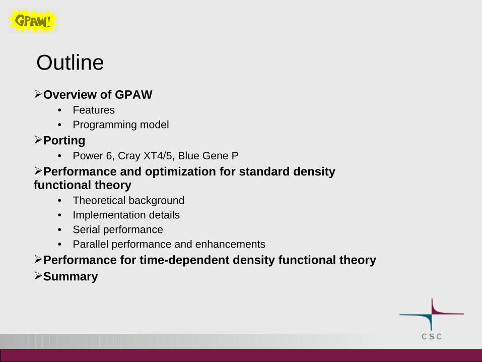
OutlineOverview of GPAW

• Features• Programming model

Porting• Power 6, Cray XT4/5, Blue Gene P

Performance and optimization for standard density functional theory

• Theoretical background• Implementation details• Serial performance• Parallel performance and enhancements

Performance for time-dependent density functional theorySummary

          

Acknowledgements All the development is done in close collaboration with the

whole GPAW development team:• Argonne National Laboratory, USA• CAMd, Technical University of Denmark• Department of Physics, Helsinki University of Technology, Finland• Department of Physics, Jyväskylä University, Finland• Freiburg Materials Research Center, Germany• Institute of Physics, Tampere University of Technology, Finland

Key developers in optimization efforts• Jens Jörgen Mortensen, DTU• Marcin Dulak, DTU• Nichols Romero, Argonne

          

GPAW Software package for quantum mechanical calculations

of nanostructures Ground state properties

• Total energies, structural optimizations, ...• Density functional theory

Excited state properties• Optical spectra, ...• Time-dependent density functional theory

System sizes up to few nm, few thousand electrons Open source software licensed under GPL

wiki.fysik.dtu.dk/gpaw 

          

Programming model: Python + C

Python• Modern, general purpose object oriented

programming language• Interpreted language• Rapid development• Easy to extend with C (and Fortran) routines

Message passing interface (MPI) Core low level routines implemented in C

• MPI-calls directly from C

High level algorithms implemented in Python

• Python interfaces to BLAS and LAPACK• Python interfaces to MPI

Execution time:

Lines of code:

Python C

C

BLAS, LAPACK, MPI, numpy

          

Programming model Python makes it easy to focus on efficient high level algorithms

Installation can be be intricate in special operating systems

• Catamount, CLE• BlueGene

Debugging and profiling tools are often only for C or Fortran programs

• C-extensions can be profiled easily• Possible to have Python-interfaces to profiling

API such as CrayPAT

# Calculate the residual of pR_G # dR_G = (H - e S) pR_G hamiltonian.apply(pR_G, dR_G, kpt) overlap.apply(pR_G, self.work[1], kpt) axpy(-kpt.eps_n[n], self.work[1], dR_G)

RdR = self.comm.sum(real(npy.vdot(R_G, dR_G)))

Python code sniplet from iterative eigensolver

          

Porting Software requirements for GPAW

• Python• Numpy (Python package for numerical computations)• LAPACK, BLAS (SCALAPACK)• MPI

Python distutils• “makefile” for numpy and GPAW• Use same compiler and options as when building Python• Straightforward installation in standard Unix-systems• Cross compilation can be more difficult

For parallel calculations GPAW uses special Python interpreter:

int main(int argc, char **argv){ int status; MPI_Init(&argc, &argv); status = Py_Main(argc, argv); MPI_Finalize(); return status;}

          

Porting to Power6 on Linux

Standard Unix system Current porting with gcc Straightforward porting wiki.fysik.dtu.dk/gpaw/install/Linux/huygens.htm

          

Porting to Cray XT

Python is not supported in Catamount or CNL operating systems No shared libraries

• Normally, the python standard library consists of pure Python modules and of C-extensions

• C-extensions are dynamically loaded libraries

All the needed C-extensions have to build statically into libpython.a

Custom dynamic Python module loader Python is needed on front end node for build process Python is need on compute nodes for calculations Once Python is ported, building Numpy and GPAW is relatively

straigthforward wiki.fysik.dtu.dk/gpaw/install/Cray/louhi.html

          

Porting to Blue Gene P

Python is supported on Blue Gene P Shared libraries are supported on Blue Gene P Python is build with gcc, using xlc for GPAW requires

conversion of gcc options to xlc options Cross compilation can be tricky:

• using accidently front-end libraries produces code which works 95 % of test cases

• it can be difficult to locate the errors to wrong libraries

wiki.fysik.dtu.dk/gpaw/install/BGP/jugene.html

          

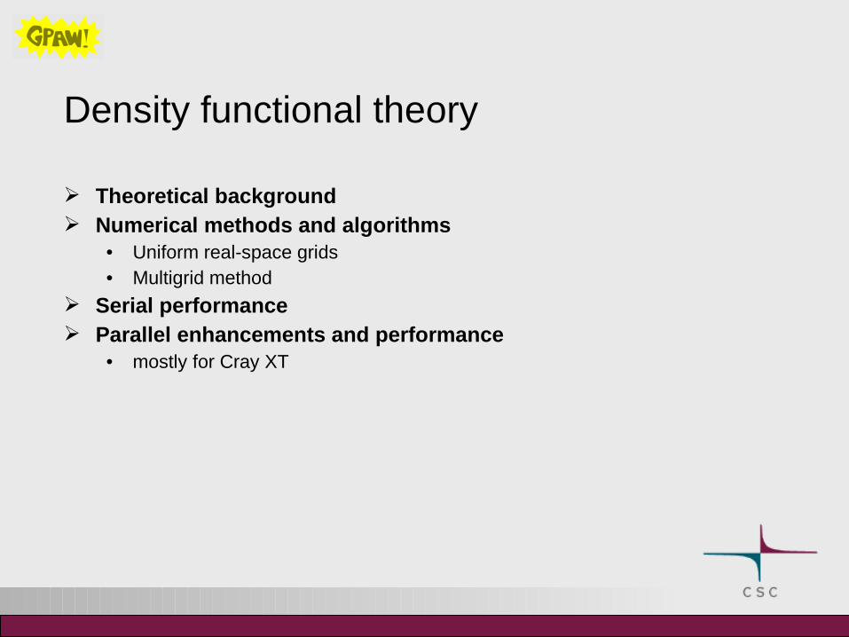
Density functional theory

Theoretical background Numerical methods and algorithms

• Uniform real-space grids• Multigrid method

Serial performance Parallel enhancements and performance

• mostly for Cray XT

          

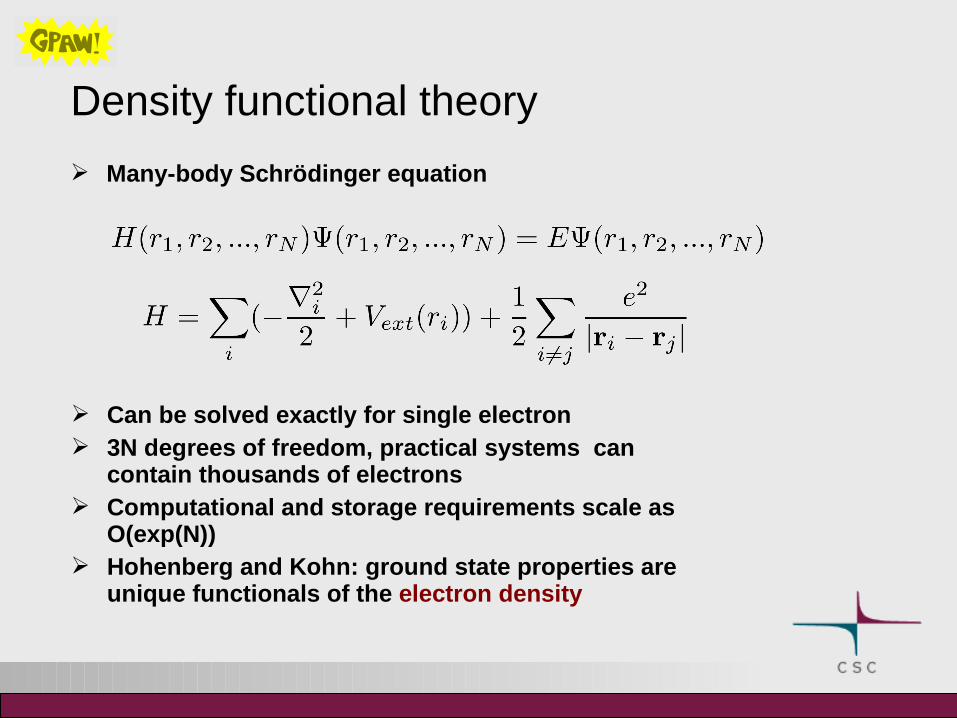
Density functional theory

Many-body Schrödinger equation

Can be solved exactly for single electron 3N degrees of freedom, practical systems can

contain thousands of electrons Computational and storage requirements scale as

O(exp(N)) Hohenberg and Kohn: ground state properties are

unique functionals of the electron density

          

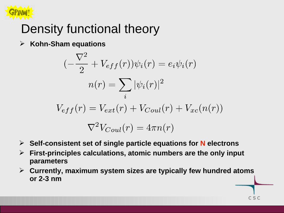
Density functional theory Kohn-Sham equations

Self-consistent set of single particle equations for N electrons First-principles calculations, atomic numbers are the only input

parameters Currently, maximum system sizes are typically few hundred atoms

or 2-3 nm

          

Projector augmented wave (PAW) method

Only valence electrons are chemically active Wave functions vary rapidly near atomic nuclei In projector augmented wave (PAW) method core electrons

are frozen and one works with smooth pseudo wave functions Wave functions and expectation values can be represented as

= + -

Smooth part Atomic corrections

PAW method introduces non-local term in effective potential

          

Real space grids Wave functions, electron densities, and potentials are represented

on uniform grids. Single parameter, grid spacing h

h

Accuracy of calculation can be improved systematically by decreasing the grid spacing

          

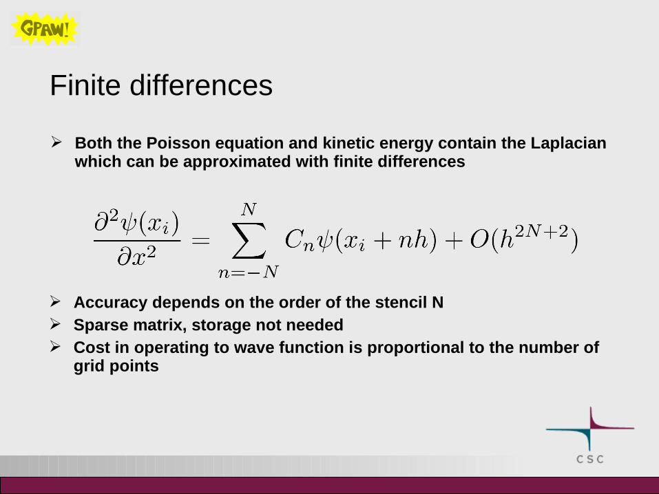
Finite differences

Both the Poisson equation and kinetic energy contain the Laplacian which can be approximated with finite differences

Accuracy depends on the order of the stencil N Sparse matrix, storage not needed Cost in operating to wave function is proportional to the number of

grid points

          

Multigrid method General framework for solving differential equations using a

hierarchy of discretizations

Recursive V-cycle Transform the original equation to a coarser

discretization• restriction operation

Correct the solution with results from coarser level

• interpolation operation

          

Self-consistency cycle0)Initial guess for the density and wave functions

1)Calculate HamiltonianPoisson equation is solved with multigridO(N) scaling with system size

2)Subspace diagonalization of wave functionsConstruct Hamiltonian matrixDiagonalize matrixRotate wave functionsO(N3) scaling

3)Iterative refinement of wave functionsPreconditioning with multigridO(N2) scaling

4)Orthonormalization of wave functionsCalculate overlap matrixCholesky decompositionRotate wave functionsO(N3) scaling

5)Calculate new charge density

6)Return to 1 until converged

          

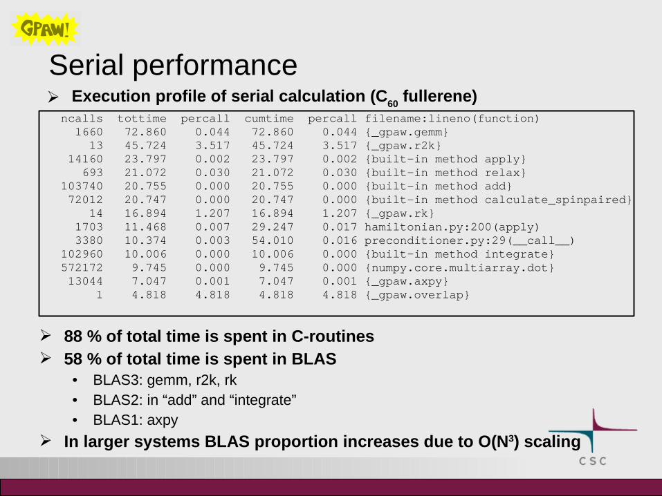
Serial performance Execution profile of serial calculation (C

60 fullerene)

ncalls tottime percall cumtime percall filename:lineno(function) 1660 72.860 0.044 72.860 0.044 {_gpaw.gemm} 13 45.724 3.517 45.724 3.517 {_gpaw.r2k} 14160 23.797 0.002 23.797 0.002 {built-in method apply} 693 21.072 0.030 21.072 0.030 {built-in method relax} 103740 20.755 0.000 20.755 0.000 {built-in method add} 72012 20.747 0.000 20.747 0.000 {built-in method calculate_spinpaired} 14 16.894 1.207 16.894 1.207 {_gpaw.rk} 1703 11.468 0.007 29.247 0.017 hamiltonian.py:200(apply) 3380 10.374 0.003 54.010 0.016 preconditioner.py:29(__call__) 102960 10.006 0.000 10.006 0.000 {built-in method integrate} 572172 9.745 0.000 9.745 0.000 {numpy.core.multiarray.dot} 13044 7.047 0.001 7.047 0.001 {_gpaw.axpy} 1 4.818 4.818 4.818 4.818 {_gpaw.overlap}

88 % of total time is spent in C-routines 58 % of total time is spent in BLAS

• BLAS3: gemm, r2k, rk• BLAS2: in “add” and “integrate”• BLAS1: axpy

In larger systems BLAS proportion increases due to O(N3) scaling

          

Parallelization strategies

Domain decomposition Parallelization over k-points and spin Parallelization over electronic states

          

Parallelization over k-points and spin

In (small) periodic systems parallelization over k-points• almost trivial parallelization• number of k-points decreases with increasing system size

Parallelization over spin in magnetic systems• almost trivial parallelization• only two spin degrees of freedom

Communication only when summing for charge density

          

Domain decomposition

Domain decomposition: real-space grid is divided to different processors

Only local communication Total amount of communication is

small Finite-difference:

• computation NG

/ P

• communication ( NG / P ) 2/3

Finite difference Laplacian

P1

P3 P4

P2

          

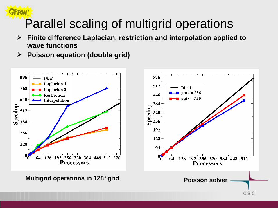
Parallel scaling of multigrid operations Finite difference Laplacian, restriction and interpolation applied to

wave functions Poisson equation (double grid)

Poisson solverMultigrid operations in 1283 grid

          

Parallel performance with domain decomposition Test system: 256 water molecules, 768 atoms, 1056

electrons, 112 x 112 x 112 grid

Problem:• Matrix diagonalization in subspace rotation takes 270 s and it is

done serially!

Solution:• Use Scalapack for diagonalization

procs time (s) speedup

128 571

256 452 1.26

          

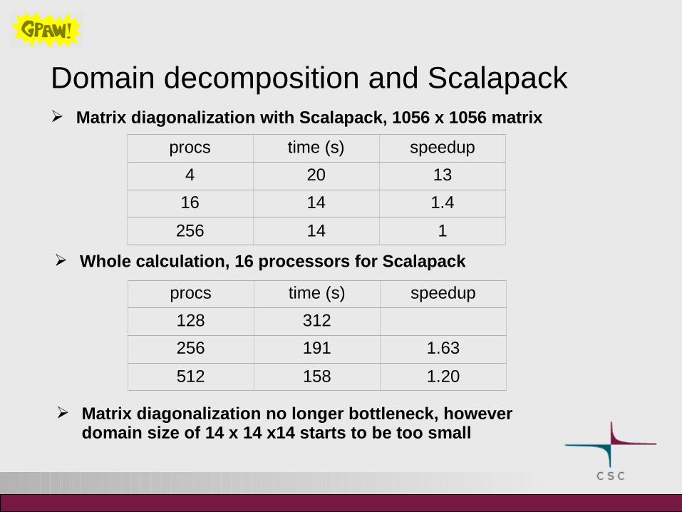
Domain decomposition and Scalapack Matrix diagonalization with Scalapack, 1056 x 1056 matrix

procs time (s) speedup

4 20 13

16 14 1.4

256 14 1

procs time (s) speedup

128 312

256 191 1.63

512 158 1.20

Whole calculation, 16 processors for Scalapack

Matrix diagonalization no longer bottleneck, however domain size of 14 x 14 x14 starts to be too small

          

Parallelization over electronic states

Non-trivial parallelization of eigenvalue problem• eigensolvers require orthonormalization• in practice, also subspace diagonalization is needed

Construction of matrices like

Matrix-vector products like

All-to-all communication of wave functions Large messages

          

Parallelization over electronic states 1D block cyclic distribution of wave functions Pipeline with overlapping computation and

communication• communication only between nearest neighbors

Example: 4 processors, 3 steps• step 0, the diagonal elements are calculated and

the same time the blocks needed for diagonal+1 elements are exchanged

• step 1, diagonal+1 elements are calculated while the next blocks are exchanged

• step 2, diagonal+2 elements are calculated while the next blocks are exchanged.

• step 3, diagonal+3 elements are calculated. For symmetric matrices step 3 is not needed

Generally, B / 2 + 1 pairs of send-receives (B=number of processors for state parallelization)

0 1 B-1...

          

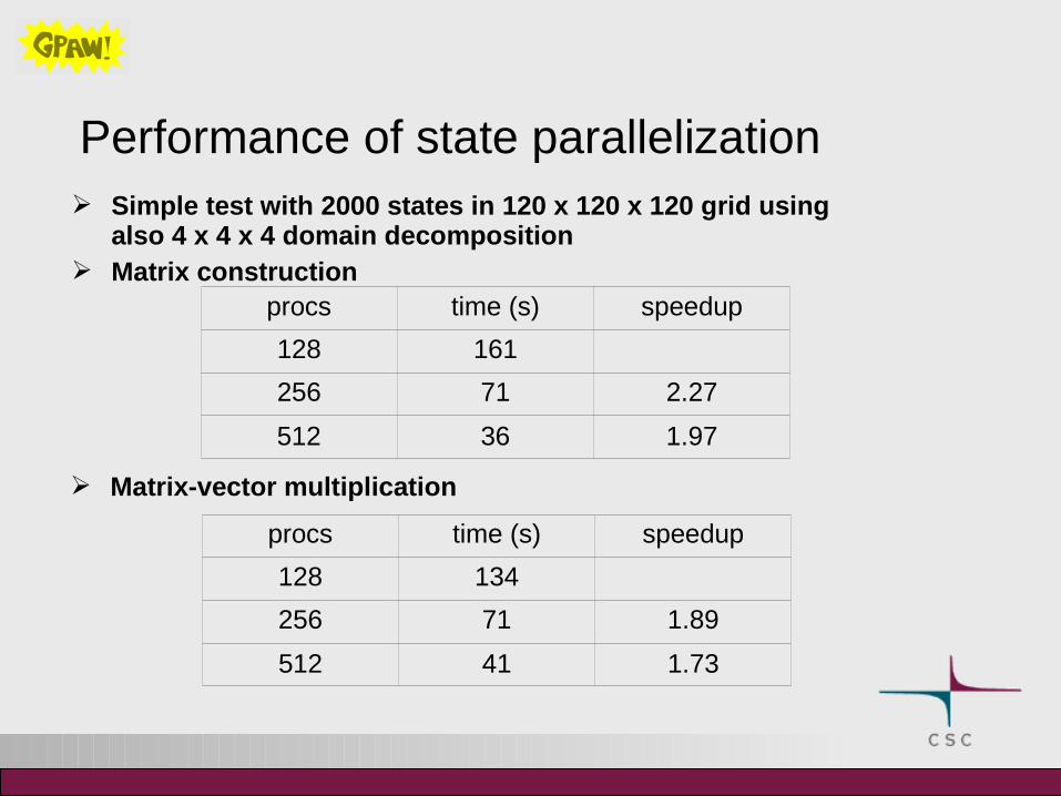
Performance of state parallelization Simple test with 2000 states in 120 x 120 x 120 grid using

also 4 x 4 x 4 domain decomposition Matrix construction

procs time (s) speedup

128 161

256 71 2.27

512 36 1.97

Matrix-vector multiplication

procs time (s) speedup

128 134

256 71 1.89

512 41 1.73

          

Rank placement

In Cray, large random variations in the execution time of matrix construction + matrix vector product

• with 512 cores, maximum time 140 s, minimum time 80 s

Ranks 0-63 contain first group of states, ranks 64-127 second group of states etc.

By default, processes are placed to nodes by increasing rank number

State parallelization involves large (10-40 MB) messages In realistic situation, bandwidth depends on physical

distance between the nodes Custom rank placement with MPICH_RANK_ORDER file:

• processes which exchange large messages are close to each other, i.e placement goes like 0,64,128,...

• coherent execution time of 75 s

          

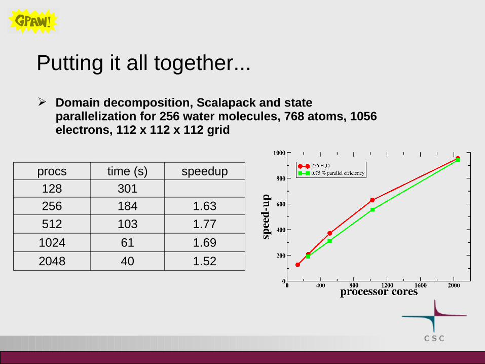
Putting it all together...

Domain decomposition, Scalapack and state parallelization for 256 water molecules, 768 atoms, 1056 electrons, 112 x 112 x 112 grid

procs time (s) speedup

128 301

256 184 1.63

512 103 1.77

1024 61 1.69

2048 40 1.52

          

Things neglected by now

Initialization phase of the calculation does not scale so well

• initial guess for the wave functions• when python is started, lots of small files are read• in Cray, startup time increases rapidly with increasing processor

count• in production calculations initialization time should not be so bad,

however in small benchmarks it can be significant

GPAW (or DFT in general) is not very IO-intensive• in practice users might want restart files• for petascale production calculations parallel IO might be

necessary

          

Limiting factors in parallel scalability

Atomic spheres are not necessarily divided evenly to domains

• load imbalance which limits scalabilty of domain decomposition

Calculation of Hamiltonian• Can be parallelized only over domains

Matrix diagonalization• Scalapack scalability is limited due to modest matrix sizes

Communication patterns of finite-difference operations are not optimal, possibility for small enhancements

          

Time-dependent density-functional theory Generalization of density-functional theory also to time-

dependent cases Excited state properties

• excited state energies• optical absorption spectra• ...

Time-dependent Kohn-Sham equations

          

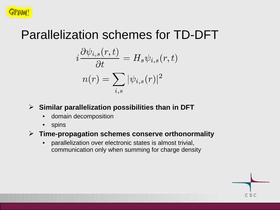
Parallelization schemes for TD-DFT

Similar parallelization possibilities than in DFT• domain decomposition• spins

Time-propagation schemes conserve orthonormality• parallelization over electronic states is almost trivial,

communication only when summing for charge density

          

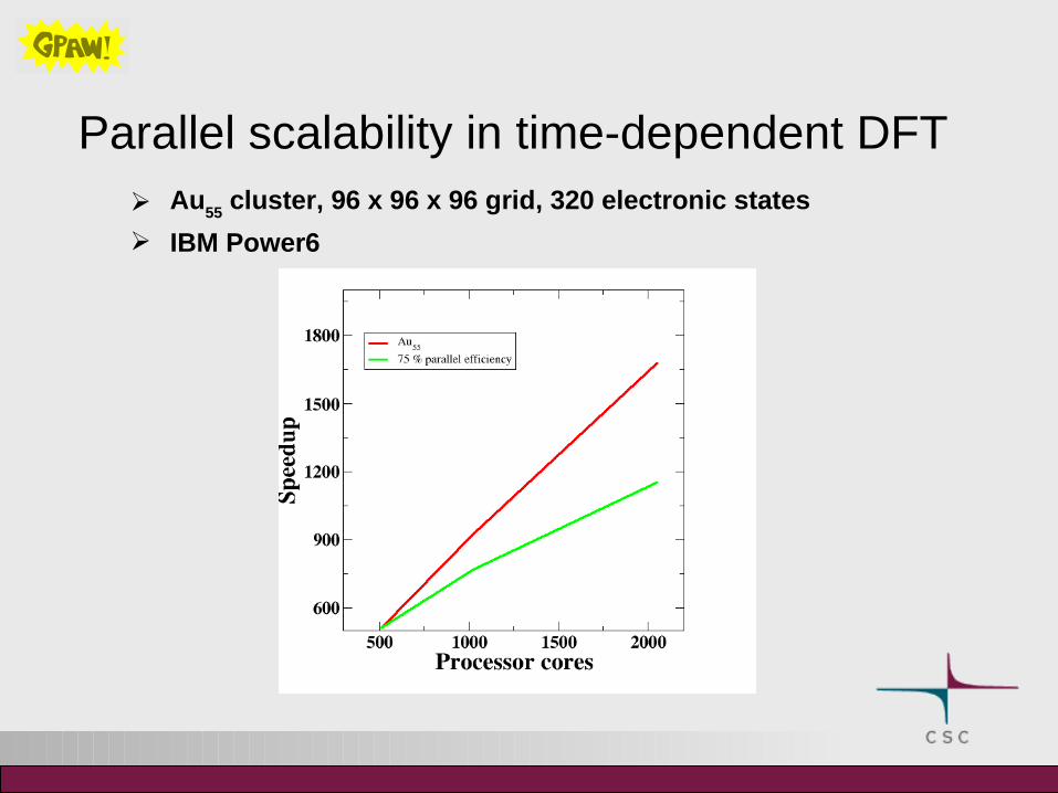
Parallel scalability in time-dependent DFT Au

55 cluster, 96 x 96 x 96 grid, 320 electronic states

IBM Power6

          

Possible enhancements for TDDFT

TD DFT uses only BLAS 1 routines, serial optimizations are more plausible than in DFT part

• Converting some Python routines to C

Optimizing communication of finite difference operations• probably larger benefits than in standard DFT

Algorithm is memory bandwidth limited, difficult to obtain very high FLOP rates

          

Summary and final thoughts Python + C programming model can be used for high

performance computing• porting especially in cross-compilation environments can be

tricky

Density functional theory code can be parallelized efficiently with multilevel parallelism

• rank placement can be important in petascale systems• large systems could scale to over 10 000 cores

Time-dependent density functional calculations scales extremely well

• 4000 cores already on relative small systems• large systems with 100 000 cores?

Good collaboration with developer community is very important