portfolio optimization with stochastic volatilities : a

IntroductionProblem formulation in the case of power utility

Characterization of the optimal investment strategyProblem formulation in the case of exponential utility

Portfolio Optimization with StochasticVolatilities : A Semi linear PDE Approach

Amina Bouzguenda Zeghal, Mohamed Mnif

Ecole Nationale d’Ingénieurs de Tunis, Tunisie

Groupe de travail de CMAP

Mohamed Mnif Portfolio Optimization



Outline

1 Introduction

2 Problem formulation in the case of power utility

3 Characterization of the optimal investment strategyVerification TheoremRegularity of the value functionExample: A multi-assets stochastic volatility modelConnection with BSDEs and numerical study

4 Problem formulation in the case of exponential utilityThe modelNumerical study




Introduction

Portfolio optimization: a fundamental concern when investorstrade between a large number of risky assets

Merton (1971): Maximizing expected utility of terminalwealthHe derived a closed formula.Many generalizations: Zariphopoulou (1994) maximizingunder Bankruptcy constraint, Akian Menaldi Sulem (1996)maximizing with transaction costs, Benth et all (2001)maximizing in pure-jump Lévy model.

Maximizing utility problems lead to HJB EquationsAn efficient algorithm: Howard algorithm computing twosequences the optimal strategy and the value function. Notpossible when risky assets number > 3 .




Introduction

Zariphopoulou (2001): maximizing utility in a market withone risky asset and a stochastic volatility model.Using a power transformation: the value function is asolution of a linear P.D.EPham (2002): multidimensional model. A powertransformation leads to a semi linear parabolic equation.Mnif ((2007): multidimensional model, stochastic volatilitymodel, exponential utility, constraints on amounts, jumpdiffusion process. When there is no correlation betweenthe risky asset and the factor volatility, the optimalinvestment strategy is determined by solving a staticoptimization problem.




Problem formulation

(Ω,F ,P) filtered probability spacefinancial market: bond S0 and n risky assets S

S0 ≡ 1dSt = diag(St−)

(b(Λt)dt + σ(Λt)dWt + σ(Λt)dWt

+

∫IRn\0

γ(Λt ,u)µ(dt ,du)

)

W d-dimensional standard Brownian motionW m-dimensional standard Brownian motion independent of Wµ a Poisson random measure andµ(dt ,du) = (µ(dt ,du))1≤i≤n = (µi(dt ,du)− qi(du)dt)1≤i≤n isthe compensated Poisson random measure




Problem formulation

qi(du) is the Lévy measure∫IRn\0

qi(du) <∞.

Λ is a d dimensional stochastic factor

dΛt = η(Λt)dt + dWt ,

Assumption (H1) η is Lipschitz.We denote

Σ(λ) = (σ(λ), σ(λ)),

α(λ) = infπ∈IRn,π 6=0

|Σ(λ)∗π|2

|π|2, λ ∈ IRd ,




Problem formulation

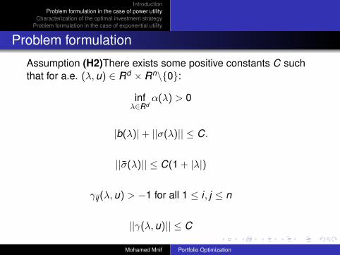
Assumption (H2)There exists some positive constants C suchthat for a.e. (λ,u) ∈ IRd × IRn\0:

infλ∈IRd

α(λ) > 0

|b(λ)|+ ||σ(λ)|| ≤ C.

||σ(λ)|| ≤ C(1 + |λ|)

γij(λ,u) > −1 for all 1 ≤ i , j ≤ n

||γ(λ,u)|| ≤ C




Problem formulation

A strategy π is said admissible if it is IF -predictable and

πt ∈ ∆ := (π1, ..., πn) ∈ [0,1]n,n∑

i=1

πi ≤ 1a.s. for all 0 ≤ t ≤ T .

A the set of admissible controls.

Xt = x +

∫ t

0Xs−

(π∗sb(Λs)ds + π∗sσ(Λs)dWs + π∗s σ(Λs)dWs

+

∫IRn\0

π∗sγ(Λs,u)µ(ds,du)

)The utility function: U(x) = xδ

δ , x ∈ IR+, The objective of theagent

v(t , x , λ) = supπ∈A

E [U(XT )|Xt = x ,Λt = λ], (t , x , λ) ∈ [0,T ]× IR+ × IRd .




Verification TheoremRegularity of the value functionExample: A multi-assets stochastic volatility modelConnection with BSDEs and numerical study

Semi-linear PDE

∂v∂t

+η(λ)∗Dλv +124λv + max

π∈∆

xπ∗b(λ)

∂v∂x

+ x2 12|Σ(λ)∗π|2∂

2v∂x2 + xπ∗σ(λ)D2

xλv

+n∑

i=1

∫IRn\0

(v(t , x(1 + π∗γi(λ,u)), λ)

− v(t , x , λ)− xπ∗γi(λ,u)∂v∂x

)qi(du)

= 0,

for a.e. (t , x , λ) ∈ [0,T )× IR+ × IRd

v(T , x , λ) =xδ

δ,





Semi-linear PDE

Due to the power utility function, we look for a candidate of HJBequation in the form:

v(t , x , λ) =xδ

δexp (−φ(t , λ)).

By differentiation, HJB implies

− ∂φ

∂t− 1

24φ+ H(λ,Dφ) = 0, (t , λ) ∈ [0,T )× IRd , , (1)

with terminal condition

φ(T , λ) = 0, y ∈ IRd , (2)





Semi-linear PDE

H is defined on IRd × IRd by

H(λ,p) =12|p|2 − p∗η(λ)

+ maxπ∈∆

δ(π∗b(λ)− π∗σ(λ)p)− 1

2δ(1− δ)|Σ(λ)∗π|2

+n∑

i=1

∫IRn\0

((1 + π∗γi(λ,u))δ − 1− δπ∗γi(λ,u)

)qi(du)

.





Semi-linear PDE

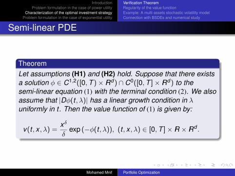
TheoremLet assumptions (H1) and (H2) hold. Suppose that there existsa solution φ ∈ C1,2([0,T )× IRd) ∩ C0([0,T ]× IRd) to thesemi-linear equation (1) with the terminal condition (2). We alsoassume that |Dφ(t , λ)| has a linear growth condition in λuniformly in t. Then the value function of (1) is given by:

v(t , x , λ) =xδ

δexp (−φ(t , λ)), (t , x , λ) ∈ [0,T ]× IR × IRd .





TheoremThe optimal portfolio is given by the Markov controlπt = π(t ,Λt),0 ≤ t ≤ T where

π(t , λ) ∈ arg minπ∈∆

−δ(π∗b(λ)− π∗σ(λ)Dφ(t , λ))

+12δ(1− δ)|Σ(λ)∗π|2

−n∑

i=1

∫IRn\0

((1 + π∗γi(λ,u))δ − 1− δπ∗γi(λ,u)

)qi(du)

.





Regularity of the value function

(H3)(i) infy∈IRd

α(y) > 0 (uniform elliptic volatility).

(ii) η is C1 and Lipschitz, b is C1 and bounded and Db isbounded.(iii)ΣΣ∗ is C1 and bounded and ||D(ΣΣ∗)|| is bounded(iv)−1 < γij(λ,u) = γij(u) ≤ M for all (λ,u) ∈ IRd × IRn \ 0where M > 0.





Regularity of the value function

Theorem

Under Assumption (H3), there exists a solutionφ ∈ C1,2([0,T )× IRd) ∩ C0([0,T ]× IRd) to the semi-linearequation (1) with terminal condition (2) and linear growthcondition in λ uniformly in t on the derivative Dφ.





dSit

Sit−

= bidt + νi(Λit)i∑

j=1

ρij(ρjdW jt +

√1− ρ2

j dW jt )

+n∑

j=1

∫IRn\0

γij(u)µj(dt ,du),

dΛit = (ai − θiΛit)dt + dW it , for all i ∈ 1, ...,n.

(νi)1≤i≤n bounded C1 functions with bounded derivatives andlower bounded by a positive constant εi > 0 for all i ∈ 1, ...,nai and θi are constants, ρij is the constant correlation betweenthe two Brownian motions of Si and Sj , ρi is the constantcorrelation between Si and its volatility and γij(u) > −1 and isbounded.





The optimal portfolio is given by:

π(t ,Λt) ∈ arg minπ∈4

[−δ

n∑i=1

πibi

+δ(1− δ)

2

n∑i,j=1

πiπj

(νi(Λit))(νj(Λjt))

inf(i,j)∑k=1

ρikρjk

+ δ

n∑i=1

i∑j=1

πiρijρj(νi(Λit))∂φ

∂λj(t ,Λt)

−n∑

i=1

∫IRn\0

((1 + π∗γi(u))δ − 1− δπ∗γi(u)

)qi(du)

].





We define two processes (Y ,Z ) by

Yt := φ(t ,Λt), Zt := Dφ(t ,Λt) for all t ∈ [0,T ].

Proposition

Suppose that Assumptions (H1), (H2) and (H3) hold. We definethe processes (Y , Z ) as follows

Yt := exp(Yt), Zt := YtZt , for all t ∈ [0,T ],

then the couple (Y , Z ) is a solution of the following BSDE

− dYt = g(Λt , Yt , Zt)dt − ZtdWt ,

with terminal condition





Proposition

YT = 1

where

g(λ, y , z) = −minπ∈∆

−δ(π∗b(λ)y − π∗σ(λ)z)

+ yδ(1− δ)

2|Σ(λ)∗π|2

− yn∑

i=1

∫IRn\0

((1 + π∗γi(u))δ − 1− δπ∗γi(u)

)qi(du)

.





Discretization and simulation of the decoupled FBSDE

Step 1. Problem discretization. (tk := kh = kTN )0≤k≤N .

ΛNl,t0 = Λl,0

ΛNl,tk+1

= ΛNl,tk + η(ΛN

l,tk )h +4Wl,k ,

4Wl,k = Wl,tk+1 −Wl,tk , 1 ≤ l ≤ d .

Y NtN = 1

Z Nl,tk =

1h

Ek (Y Ntk+14Wl,k ),

Y Ntk = Ek (Y N

tk+1) + hEk (g(ΛN

tk , YNtk+1

, Z Ntk )),

where Ek (.) = E(.|Ftk ).Mohamed Mnif Portfolio Optimization




Error induced the discretization in time

Remark

Since Y NtN is a constant and ΛN is a Markov Chain, it is easy to

see that Y Ntk = yN

k (ΛNtk ) and Z N

tk = zNk (ΛN

tk ) where yNk and zN

k areunknown regression functions defined in a backward manner.

Zhang (2004), Bouchard and Touzi (2004), Gobet et al. (2005)proved For h small enough

Theorem

max0≤k≤N

E |Ytk − Y Ntk |

2 +N−1∑k=0

∫ tk+1

tkE |Zt − Z N

tk |2dt ≤ C

(1 + |Λ0|2

)h.






Step 2. Localization. Localization of the Brownian incrementsand the function g

[4Wl,k ]w = −R0√

(h) ∨4Wl,k ∧ R0√

(h)

gR(λ, y , z) = gR(−R1 ∨ λ1 ∧ R1, ...,−Rd ∨ λd ∧ Rd , y , z)

The localization modifies the numerical scheme. We define(Y N,R, Z N,R) by

Y N,RtN = 1

Z N,Rl,tk

=1h

Ek (Y N,Rtk+1

[4Wl,k ]w ),

Y N,Rtk = Ek (Y N,R

tk+1) + hEk (gR(ΛN

tk , YN,Rtk+1

, Z N,Rtk )),






RemarkThe main interest of the localization is to provide boundedregression functions yN,R

k and zN,Rk . One has

||yN,Rk ||∞ ≤ Cy (R) and ||zN,R

k ||∞ ≤ Cz(R)( See Proposition 1(Lemor Gobet and Warin (2006))

Step 3. Function bases.We approximate Y N,R

tk and Z N,Rl,tk

for all 1 ≤ l ≤ d by a

projection on a finite-dimensional function bases p0,k (ΛN,Rtk )

and pl,k (ΛN,Rtk ) for all 1 ≤ l ≤ d .

We set αl,k for all 0 ≤ l ≤ d the projection coefficients ofY N,R

tk and Z N,Rl,tk

, 1 ≤ l ≤ d on the function bases(pl,k )0≤l≤d . We denote by Kl,k the size of pl,k .






Step 4. Monte-Carlo Simulations.We simulate M independent Monte Carlo simulations of(ΛN

tk )0≤k≤N and (4Wk )0≤k≤N−1. We denote(ΛN,m

tk )1≤m≤M,0≤k≤N and (4W mk )1≤m≤M,0≤k≤N−1 these

simulations.We write pl,k (ΛN,m

tk ) = pml,k and BM

l,k the matrix of sizeM × Kl,k which rows are (pm

l,k )∗. we denote by K Ml,k the rank

of BMl,k .

Step 5. Truncations. We force our approximation of Y N,R andZ N,R to be bounded by Cy (R) and Cz(R). For a function ψ, wedefine the truncations by [ψ]y (x) = −Cy (R) ∨ ψ(x) ∧Cy (R) and[ψ]z(x) = −Cz(R) ∨ ψ(x) ∧ Cz(R)





The algorithm

→ Y N,R,MtN = 1

→ iteration: for k = N − 1, ...,0, assume that yN,R,M(ΛNtk+1

) isknown, then we solve the d + 1 least-squares problems:

αMl,k = arg inf

α

1M

M∑m=1

|yN,R,Mk+1 (ΛN,m

tk+1)[4W m

l,k ]w

h− α.pm

l,k |2

αM0,k = arg inf

α

1M

M∑m=1

|yN,R,M(ΛN,mtk+1

)

+ hgR(ΛN,mtk , yN,R,M

k+1 (ΛN,mtk+1

), [αMl,k .p

ml,k ]z)− α.pm

0,k |2

→ yN,R,Mk (.) = [αM

0,k .p0,k ]y (.) and zN,R,Mk (.) = [αM

l,k .pl,k ]z(.).





The algorithm

Assumption (H4) (pl,k )0≤l≤d ,0≤k≤N is a complete orthonormalsystem with respect to the empirical scalar product < ., . >k ,M

< ψ1, ψ2. >k ,M=1M

M∑m=1

ψ1(ΛN,mtk )ψ2(Λ

N,mtk )

→ (BMl,k )∗(BM

l,k )

M = Id

αMl,k =

1M

M∑m=1

pml,k yN,R,M

k+1 (ΛN,mtk+1

)[4W m

l,k ]w

h

αM0,k =

1M

M∑m=1

pm0,k

(yN,R,M

k+1 (ΛN,mtk+1

)

+ hgR(ΛN,mtk , yN,R,M

k+1 (ΛN,mtk+1

), [αMl,k .p

ml,k ]z)

)Mohamed Mnif Portfolio Optimization




The algorithm

For the convergence, we refer to Lemor, Gobet Warin(2006)The error induced by the localization has a contribution oforder hWe choose the hypercube basis. We choose a domain Dand we partition it into small hypercubes of edge κTo get a global (squared) error of order hβ, β ∈ (0,1], wehave to choose κ ≈ h

β+12 (i.e. K ≈ Ch−

d(β+1)2 )and

M ≈ Ch−d(β+1)−(β+2)log(h−d(β+1)

4 −β+12 )





Numerical Approach

We simulate the d-dimensional stochastic factor Λ = (Λt)t∈[0,T ]

by using Monte-Carlo method. We denote by ΛN,mtk ∈ IRd the

m-th approximation of Λt . We determine dmaxi,k = max

1≤m≤MΛN,m

i,tk

and dmini,k = min

1≤m≤MΛN,m

i,tk. We consider

Dk =λ ∈ IRd , λi ∈ [dmin

i,k ,dmaxi,k ], s.t. for all 1 ≤ i ≤ d

.

We partition into small hypercubes of edge κ the domain Dk .





Two risky assets model results

dS1t

S1t

= b1dt + ν1(Λ1t)(ρ1dW 1t +

√1− ρ2

1dW 1t ),

dS2t

S2t

= b2dt + ν2(Λ2t)

(ρ(ρ1dW 1

t +√

1− ρ21dW 1

t )

+√

1− ρ2(ρ2dW 2t +

√1− ρ2

2dW 2t )

),

dΛ1t = (a1 − θ1Λ1t)dt + dW 1t , Λ10 = 0,

dΛ2t = (a2 − θ2Λ2t)dt + dW 2t , Λ20 = 0,

where νi(λ) = εi + 1√λ2+β2

i, i ∈ 1,2. Our model parameters

are given in Table 1.






Table: Values for the model’s parameters

d T h b1 b2 a1 θ1 a22 1 0.05 0.04 0.05 0.05 1 0.05θ2 ρ ρ1 ρ2 δ ε1 ε2 β1 β21 0.3 0.75 0.5 0.5 0.001 0.001 4 3

We determine Y0, then v1(0, x ,Λ0) := xδ

δ exp (−Y0). We

compute v2(0, x ,Λ0) := 1M

M∑m=1

U(X mT ), where

X mT = x +

N−1∑k=0

X mtk π

mtk

Smtk+1

− Smtk

Smtk

.






Table: Results for the value function

M 6000 8000 10000v1(0,10,Λ0) 6.391 6.413 6.415v2(0,10,Λ0) 6.391 6.412 6.416

The optimal investment strategy at t = 0 is given byπ∗0 = (0,0.56,0.44).




Numerical study

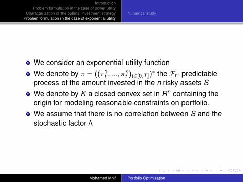
We consider an exponential utility functionWe denote by π = ((π1

t , ..., πnt )t∈[0,T ])

∗ the Ft - predictableprocess of the amount invested in the n risky assets SWe denote by K a closed convex set in IRn containing theorigin for modeling reasonable constraints on portfolio.We assume that there is no correlation between S and thestochastic factor Λ




Numerical study

Power utility maximization problem

Theorem

π(Λt) ∈ arg minπ∈K

[−δ

n∑i=1

πibi

+δ2

2

n∑i,j=1

πiπj

√(νi(Λit))√

(νj(Λjt))

inf(i,j)∑k=1

ρikρjk

+

n∑i=1

∫IRn\0

(exp (−δπ∗γi(z))− 1 + δπ∗γi(z)) qi(dz)

],

a.s.,0 ≤ t ≤ T .




Numerical study


ν(dt ,dz) is a Poisson process with constant intensity q.All the claims have the same size denoted by γ.K = IRn

+.

minπ∈K

f (π),

where

f (π) := −δπ∗b + δ2

2 |Σ(λ)∗π|2 +n∑

i=1

qi(exp (−δπ∗γi)− 1 + δπ∗γi).




Numerical study


The algorithmInitialization: Choose π0 ∈ IRn

+. Set k = 0, kcycle := 1, and

I0 := 1 ≤ i ≤ n; π0i = 0; J0 := 1, . . . ,n \ I0.

Step 1: Compute the reduce Newton direction dk , defined by

dk := −(

D2πJk

,πJkf (πk )

)−1Dπk

Jkf (πk ),

and the maximum non-negative feasible step ρkMax along dk ,

not greater than 1:

ρkMax := min

(1,min

−πk

i

dki

; dki < 0, i ∈ Jk

).




Numerical study

Step 2: Perform an Armijo type linesearch, i.e., choose thegreatest step αk ∈ (0, ρk

Max), of the form β jkρkMax for some

jk ∈ IN, for which it holds that

f (πk + αkdk ) ≤ f (πk ) + wαkDπf (πk )dk . (3)

Step 3: Update Jk and Ik : Set Ik+1 := Ik and Jk+1 := Jk , and foreach i ∈ Jk such that πi + αkdk

i = 0, do Jk+1 := Jk \ i andIk+1 := Ik ∪ i.Step 4: Update of current point: set πk+1 := πk + αkdk , andk := k + 1.Step 5: Test of end of cycle: if∥∥∥DπJ f (πk ))

∥∥∥ ≤ ε1/2kcycle ,

go to step 6. Otherwise, go to step 1.




Numerical study

Step 6: Stopping test: let i0 ∈ Ik be such that

Dπi0f (πk ) = min

(Dπi f (π

k ))

; i ∈ Ik.

If Dπi0f (πk ) ≥ −ε2, stop.

Step 7: Start a new cycle. Set kcycle := kcycle + 1 and compute

Jk := Jk∪i0; Ik := Ik\i0; d := −(

D2πJk

,πJkf (π)

)−1DπJk

f (π).

If di0 < 0, set Ik := Ik ∪ i0 and Jk := Jk \ i0.Go to step 1.




Numerical study

Numerical results

the matrix of correlation is given by

1 0 0 0 0 0 0 0 0 00.5 0.86 0 0 0 0 0 0 0 00.25 0.25 0.93 0 0 0 0 0 0 0

0 0 0.86 0.5 0 0 0 0 0 00 0 0 0.86 0.5 0 0 0 0 00 0 0 0 0.86 0.5 0 0 0 00 0 0 0 0 0.86 0.5 0 0 00 0 0 0 0 0 0.86 0.5 0 00 0 0 0 0 0 0 0.86 0.5 00 0 0 0 0 0 0 0 0.86 0.5

.




Numerical study

Numerical results

The matrix parameterizing the jumps is given by

0.15 0.15 0.15 0.15 0.15 0.15 0.15 0.15 0.15 0.150.3 0.3 0.3 0.3 0.3 0.3 0.3 0.3 0.3 0.30.1 0.1 0.1 0.1 0.1 0.1 0.1 0.1 0.1 0.10.1 0.1 0.1 0.1 0.1 0.1 0.1 0.1 0.1 0.10.1 0.1 0.1 0.1 0.1 0.1 0.1 0.1 0.1 0.10.1 0.1 0.1 0.1 0.1 0.1 0.1 0.1 0.1 0.10.1 0.1 0.1 0.1 0.1 0.1 0.1 0.1 0.1 0.10.1 0.1 0.1 0.1 0.1 0.1 0.1 0.1 0.1 0.10.1 0.1 0.1 0.1 0.1 0.1 0.1 0.1 0.1 0.10.4 0.4 0.4 0.4 0.4 0.4 0.4 0.4 0.4 0.4

.




Numerical study

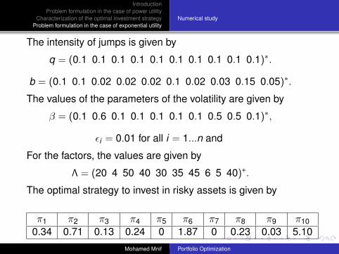
The intensity of jumps is given by

q = (0.1 0.1 0.1 0.1 0.1 0.1 0.1 0.1 0.1 0.1)∗.

b = (0.1 0.1 0.02 0.02 0.02 0.1 0.02 0.03 0.15 0.05)∗.

The values of the parameters of the volatility are given by

β = (0.1 0.6 0.1 0.1 0.1 0.1 0.1 0.5 0.5 0.1)∗,

εi = 0.01 for all i = 1...n and

For the factors, the values are given by

Λ = (20 4 50 40 30 35 45 6 5 40)∗.

The optimal strategy to invest in risky assets is given by

π1 π2 π3 π4 π5 π6 π7 π8 π9 π100.34 0.71 0.13 0.24 0 1.87 0 0.23 0.03 5.10

Table: The optimal strategy of investment in risky assets (test 1)Mohamed Mnif Portfolio Optimization

portfolio optimization with stochastic volatilities : a

Documents