unit tests for stochastic optimization

8/12/2019 Unit Tests for Stochastic Optimization

http://slidepdf.com/reader/full/unit-tests-for-stochastic-optimization 1/12

a r X i v : 1 3 1

2 . 6 0 5 5 v 2

[ c s . L G ]

7 J a n 2 0 1 4

Unit Tests for Stochastic Optimization

Tom Schaul Ioannis Antonoglou

DeepMind Technologies130 Fenchurch Street, London

{tom,ioannis,david}@deepmind.com

David Silver

Abstract

Optimization by stochastic gradient descent is an important component of manylarge-scale machine learning algorithms. A wide variety of such optimizationalgorithms have been devised; however, it is unclear whether these algorithms arerobust and widely applicable across many different optimization landscapes. Inthis paper we develop a collection of unit tests for stochastic optimization. Eachunit test rapidly evaluates an optimization algorithm on a small-scale, isolated,and well-understood difficulty, rather than in real-world scenarios where manysuch issues are entangled. Passing these unit tests is not sufficient, but absolutelynecessary for any algorithms with claims to generality or robustness. We giveinitial quantitative and qualitative results numerous established algorithms. Thetesting framework is open-source, extensible, and easy to apply to new algorithms.

1 Introduction

Stochastic optimization [1] is among the most widely used components in large-scale machine learn-ing, thanks to its linear complexity, efficient data usage, and often superior generalization [2, 3, 4].In this context, numerous variants of stochastic gradient descent have been proposed, in order toimprove performance, robustness, or reduce tuning effort [5, 6, 7, 8, 9]. These algorithms mayderive from simplifying assumptions on the optimization landscape [10], but in practice, they tendto be used as general-purpose tools, often outside of the space of assumptions their designers in-tended. The troublesome conclusion is that practitioners find it difficult to discern where potentialweaknesses of new (or old) algorithms may lie [11], and when they are applicable – an issue thatis separate from raw performance. This results in essentially a trial-and-error procedure for find-ing the appropriate algorithm variant and hyper-parameter settings, every time that the dataset, lossfunction, regularization parameters, or model architecture change [12].

The objective of this paper is to establish a collection of benchmarks to evaluate stochastic opti-mization algorithms and guide algorithm design toward robust variants. Our approach is akin to

unit testing, in that it evaluates algorithms on a very broad range of small-scale, isolated, and well-understood difficulties, rather than in real-world scenarios where many such issues are entangled.Passing these unit tests is not sufficient, but absolutely necessary for any algorithms with claims togenerality or robustness. This is a similar approach to the very fruitful one taken by the black-boxoptimization community [13, 14].

The core assumption we make is that stochastic optimization algorithms are acting locally, that is,they aim for a short-term reduction in loss given the current noisy gradient information, and possi-bly some internal variables that capture local properties of the optimization landscape. This propertystems from computational efficiency concerns, but it has the additional benefits of minimizing ini-tialization bias and allowing for non-stationary optimization. We therefore concentrate on buildinglocal unit tests, that investigate algorithm dynamics on a broad range of local scenarios, because

1

http://arxiv.org/abs/1312.6055v2



































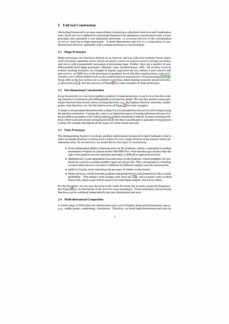
Figure 1: Some one-dimensional shape prototypes. The first six example shapes are atomic pro-totypes: a quadratic bowl, an absolute value, a cliff with a non differential point after which thederivative increases by a factor ten, a rectified linear shape followed by a bend, an inverse Gaus-sian, an inverse Laplacian. The next six example shapes are concatenations of atomic prototypes:a sigmoid as a concatenation of a non convex Gaussian a line and an exponential, a quadratic bowlfollowed by a cliff and then by an exponential function, a quadratic bowl followed by a cliff andanother quadratic bowl, a sinusoid as a concatenation of quadratic bowls, a line followed by a Gaus-sian bowl, a quadratic bowl and a cliff and finally, a Laplace bowl followed by a cliff and anotherLaplace bowl.

we expect that detecting local failure modes will flag an algorithm as unlikely to be robust on morecomplex tasks.

Our divide-and-conquer approach consists of disentangling potential difficulties and testing them inisolation or in simple couplings. Given that our unit tests are small and quick to evaluate, we canhave a much larger collection of them, testing hundreds of qualitatively different aspects in less timethan it would take to optimize a single traditional benchmark to convergence, thus allowing us tospot and address potential weaknesses early.

Our main contribution is a testing framework, with unit tests designed to test aspects such as: dis-continuous or non-differentiable surfaces, curvature scales, various noise conditions and outliers,saddle-points and plateaus, cliffs and asymmetry, and curl and bootstrapping. It also allows testcases to be concatenated by chaining them in a temporal series, or by combining them into multi-dimensional unit tests (with or without variable coupling). We give initial quantitative and qualitativeresults on a number of established algorithms.

We do not expect this to replace traditional benchmark domains that are closer to the real-world, butto complement it in terms of breadth and robustness. We have tried to keep the framework generaland extendable, in the hope it will further grow in diversity, and help others in doing robust algorithmdesign.

2



Figure 2: Examples of noise applied on prototype functions, green dashed are typical sample gra-

dients, and the standard deviation range is the blue area. The upper two subplots depict Gaussianadditive noise, while the lower two show Gaussian multiplicative noise. In the left column, thenoise is applied to the gradients of a quadratic bowl prototype (note how the multiplicative noisegoes to zero around the optimum in the middle), and on the right it is applied to a concatenation of prototypes.

composing together one-dimensional unit tests. For example for two one-dimensional prototype

shapes La and Lb combined with a p-norm, the composition is L(a,b)(θ) = (La(θ1) p + Lb(θ2) p)1p .

Noise prototypes are composed independently of shape prototypes. While they may be composedof concatenated one-dimensional prototypes, higher-dimensional prototypes are not concatenatedthemselves. Various levels of conditioning can be achieved by having dramatically different scalesin different component dimensions.

In addition to the choice of prototypes to be combined, and their scale, we permit a rotation ininput space, which couples the dimensions together and avoids axis-alignment. These rotations areparticularly important for testing diagonal/element-wise optimization algorithms.

2.5 Curl

In reinforcement learning a value function (the expected discounted reward for each state) can belearned using temporal-difference learning (TD), an update procedure that uses bootstrapping: i.e.it pulls the value of the current state towards the value of its successor state [ 19]. These stochasticupdate directions are not proper gradients of any scalar energy field [20], but they still form a (moregeneral) vector field with non-zero curl, where the objective for the optimization algorithm is toconverge to its fixed-point(s). See Figure 4 for a detailed example. We implemented this aspect byallowing different amounts of curl to be added on top of a multi-dimensional vector field in our unittests, which is done by rotating the produced gradient vectors using a fixed rotation matrix.

2.6 Non-stationarity

In many settings it is necessary to optimize a non-stationary objective function. This may typicallyoccur in a non-stationary task where the problem to be solved changes over time. However, non-stationary optimization can even be important in large stationary tasks, when the algorithm itself chooses to track a particular aspect of the problem, rather than solve the problem globally [21]. Inaddition, reinforcement learning (RL) tasks often involve non-stationary optimization. For example,many RL algorithms proceed by evaluating the value function using the TD algorithm described inthe previous section. This results in two sources of non-stationarity: the target value changes atevery step (resulting in the previously described curl); and also the state distribution changes as the

4



Figure 3: Examples of multivariate prototypes. The first subplot depicts an asymmetric quadraticbowl with correlated dimensions, the second a surface with a saddle point, the third a sharp valleysurface, the fourth a half-pipe surface where the first dimension is a line and the second one aquadratic bowl. The fifth subplot depicts a surface with an ill conditioned minimum in the pointwhere the two canyons overlap. The surface in the last subplot is the composition of a quadraticbowl in the first dimension and of a cliff in the second.

Figure 4: Here, we consider a very simple Markov process, with two states and stochastic transitionsbetween them, and a reward of 0 in the first and of 1 in the second state. Consider the parametersof our optimization θ to be the two state values. Each TD update changes one of them, dependingon the stochastic transition observed. In this figure, we plot the vector field of expected updatedirections (blue arrows) as a function of θ, as well as one sampled trajectory of the TD algorithm.Note how this vector field is not actually a gradient field, but instead has substantial curl, making ita challenging stochastic optimization task.

value function improves and better actions are selected. These scenarios can be therefore be viewedas a non-stationary loss functions, but whose optimum moves as a function of the current parametervalues.

To test non-stationarity, we allow the location of the optimum to move smoothly via a translationof the parameter space, for various movement speeds, and for various levels of stochasticity in its

5



Figure 5: Qualitative results for all algorithm variants (350) on all unit tests (800 one-dimensional ones and 200 two-dimensiones). Each column is one unit test, organized by type, and each group of rows is one algorithm, with one set of hyper-param

red/violet=divergence, orange=slow, yellow=variability, green=acceptable, blue=excellent (see main text for details).

7



Figure 6: Illustration of the loss surface of a one-dimensional auto-encoder, as defined in the text,where the darkest blue corresponds to the lowest loss. Left: from the zoomed-out perspective if ap-pears to be roughly a vertical valley, leading an optimizer toward the y-axis from almost anywhere inthe space. Center: the zoomed-in perspective around the origin, which is looking like a prototypicalsaddle point. Right: the shape of the valley in the lower left quadrant, the walls of which becomesteeper the more the search progresses.

indicate that it is difficult to substantially beat well-tuned SGD in performance on most unit tests.

Another unsurprising conclusion is that hyper-parameter tuning matters much less for the adaptivealgorithms (ADAGRAD, ADADELTA, RPROP, RMSprop) than for the non-adaptive SGD variants.Also, while some unit tests are more tricky than others on average, there is quite some diversity inthe sense that some algorithms may outdo SGD on a unit test where other algorithms fail (especiallyon the non-differentiable functions).

4 Realism and Future Work

We do not expect to replace real-world benchmark domains, but rather to complement them with oursuite of unit tests. Still, it is important to have sufficient coverage of the types of potential difficultiesencountered in realistic settings. To a much lesser degree, we may not want to clutter the test suitewith unit tests that measure issues which never occur in realistic problems.

It is not straightforward to map very high-dimensional real-world loss functions down to low-

dimensional prototype shapes, but it is not impossible. For example, in Figure 7 we show somerandom projections in parameter space of the loss function in an MNIST classification task with anMLP [28]. We defer a fuller investigation of this type, namely obtaining statistics on how commonlydifferent prototypes are occurring, to future work.

However, the unit tests capture the properties of some examples that can be analyzed. One of themwas discussed in section 2.5, another one is the simple loss function of a one-dimensional auto-encoder:

Lθ(x) = (x + θ2 · σ(x · θ1))2

where σ is the sigmoid function. Even in the absence of noise, this minimal scenario has a saddle-point near θ = (0, 0), a plateau shape away from the axes, a cliff shape near the vertical axis, anda correlated valley near θ = (1, 1), as illustrated in Figure 6. All of these prototypical shapes areincluded in our set of unit tests.

An alternative approach is predictive: if the performance on the unit tests is highly predictive of an algorithm’s performance on a some real-world task, then those unit tests must be capturing theessential aspects of the task. Again, building such a predictor is an objective for future work.

4.1 Algorithm Dynamics

Our long-term objective is to be able to do systematic testing and a full investigation of the opti-mization dynamics for a given algorithm. Of course, it is not possible to test it exhaustively on allpossible loss functions (because there are infinitely many), but a divide-and-conquer approach maybe the next best thing. For this, we introduce the notion of algorithm state, which is changing duringoptimization (e.g., the current stepsize or momentum). Now, a long optimization process can beseen as the chaining of a number of unit tests, while preserving the algorithm state in-between them.

8



Figure 7: Left: collection of 64 random projections into two dimensions of the MNIST loss sur-face (based on one randomly sampled digit for each column). The projections are centered aroundthe weights learned after one epoch of training, and different projections are plotted on scales be-tween 0.05 (top row) and 0.5 (bottom row). Right: the same as on the left, but with axis-alignedprojections.

Our hypothesis is that the set of all possible chains of unit tests in our collection covers most of thequalitatively different (stationary or non-stationary) loss functions an optimization algorithm mayencounter.

To evaluate an algorithm’s robustness (rather than its expected performance), we can assume thatan adversary picks the worst-case unit tests at each step in the sequence. An algorithm is onlytruly robust if it does not diverge under any sequence of unit tests. Besides the worst-case, we mayalso want to study typical expected behavior, namely whether the dynamics have an attractor in thealgorithm’s state space. If an attractor exists where the algorithm is stable, then it becomes usefulto look at the secondary criterion for the algorithm, namely its expected (normalized) performance.We conjecture that this analysis may lead to novel insights into how to design robust and adaptiveoptimization algorithms.

5 Conclusion

This paper established a large collection of simple comparative benchmarks to evaluate stochasticoptimization algorithms, on a broad range of small-scale, isolated, and well-understood difficulties.This approach helps disentangle issues that tend to be confounded in real-world scenarios, whileretaining realistic properties. Our initial results on a dozen established algorithms (under a variety of different hyperparameter settings) show that robustness is non-trivial, and that different algorithmsstruggle on different unit tests. The testing framework is open-source, extensible to new functionclasses, and easy to use for evaluating the robustness of new algorithms.

The full source code (see also Appendix A) is available under BSD license at:

https://github.com/IoannisAntonoglou/optimBench

References

[1] H. Robbins and S. Monro. A stochastic approximation method. Annals of MathematicalStatistics, 22:400–407, 1951.

[2] Leon Bottou. Online Algorithmsand Stochastic Approximations. In David Saad, editor, Online Learning and Neural Networks. Cambridge University Press, Cambridge, UK, 1998.

9



[3] Leon Bottou and Yann LeCun. Large Scale Online Learning. In Sebastian Thrun, LawrenceSaul, and Bernhard Scholkopf, editors, Advances in Neural Information Processing Systems16 . MIT Press, Cambridge, MA, 2004.

[4] Leon Bottou and Olivier Bousquet. The Tradeoffs of Large Scale Learning. In J.C. Platt,D. Koller, Y. Singer, and S. Roweis, editors, Advances in Neural Information Processing Sys-tems, volume 20, pages 161–168. NIPS Foundation (http://books.nips.cc), 2008.

[5] A. Benveniste, M. Metivier, and P. Priouret. Adaptive Algorithms and Stochastic Approxima-tions. Springer Verlag, Berlin, New York, 1990.

[6] N. Le Roux, P.A. Manzagol, and Y. Bengio. Topmoumoute online natural gradient algorithm,2008.

[7] Antoine Bordes, Leon Bottou, and Patrick Gallinari. SGD-QN: Careful Quasi-NewtonStochastic Gradient Descent. Journal of Machine Learning Research, 10:1737–1754, July2009.

[8] Wei Xu. Towards Optimal One Pass Large Scale Learning with Averaged Stochastic GradientDescent. ArXiv-CoRR, abs/1107.2490, 2011.

[9] Tom Schaul, Sixin Zhang, and Yann LeCun. No More Pesky Learning Rates. In InternationalConference on Machine Learning (ICML), 2013.

[10] John C. Duchi, Elad Hazan, and Yoram Singer. Adaptive Subgradient Methods for OnlineLearning and Stochastic Optimization. 2010.

[11] Razvan Pascanu, Tomas Mikolov, and Yoshua Bengio. Understanding the exploding gradientproblem. arXiv preprint arXiv:1211.5063, 2012.

[12] X. Glorot and Y. Bengio. Understanding the difficulty of training deep feedforward neuralnetworks. In G. Orr and Muller K., editors, Proceedings of the International Conference on Artificial Intelligence and Statistics (AISTATS), pages 249–256. Society for Artificial Intelli-gence and Statistics, 2010.

[13] Nikolaus Hansen, Anne Auger, Steffen Finck, Raymond Ros, et al. Real-parameter black-boxoptimization benchmarking 2010: Experimental setup. 2010.

[14] Nikolaus Hansen, Anne Auger, Raymond Ros, Steffen Finck, and Petr Posık. Comparingresults of 31 algorithms from the black-box optimization benchmarking BBOB-2009. In Pro-ceedings of the 12th annual conference companion on Genetic and evolutionary computation,

pages 1689–1696. ACM, 2010.

[15] Alex Krizhevsky, Ilya Sutskever, and Geoff Hinton. Imagenet classification with deep con-volutional neural networks. In Advances in Neural Information Processing Systems 25, pages1106–1114, 2012.

[16] Ian J Goodfellow, David Warde-Farley, Mehdi Mirza, Aaron Courville, and Yoshua Bengio.Maxout networks. arXiv preprint arXiv:1302.4389, 2013.

[17] Y. LeCun, L. Bottou, G. Orr, and K. Muller. Efficient BackProp. In G. Orr and Muller K.,editors, Neural Networks: Tricks of the trade. Springer, 1998.

[18] Geoffrey E Hinton, Nitish Srivastava, Alex Krizhevsky, Ilya Sutskever, and Ruslan R Salakhut-dinov. Improving neural networks by preventing co-adaptation of feature detectors. arXiv preprint arXiv:1207.0580, 2012.

[19] R.S. Sutton and A.G. Barto. Reinforcement Learning: An Introduction. IEEE Transactions on

Neural Networks, 9(5):1054–1054, Sep 1998.

[20] Etienne Barnard. Temporal-difference methods and Markov models. IEEE Transactions onSystems, Man, and Cybernetics, 23(2):357–365, 1993.

[21] Richard S. Sutton, Anna Koop, and David Silver. On the role of tracking in stationary environ-ments. In Proceedings of the Twenty-Fourth International Conference on Machine Learning(ICML 2007 , pages 871–878. ACM Press, 2007.

[22] Yurii Nesterov and Arkadii Semenovich Nemirovskii. Interior-point polynomial algorithms inconvex programming, volume 13. SIAM, 1994.

[23] Matthew D Zeiler. ADADELTA: An Adaptive Learning Rate Method. arXiv preprint arXiv:1212.5701, 2012.

10



[24] Richard S Sutton. Adapting bias by gradient descent: An incremental version of delta-bar-delta. In AAAI , pages 171–176, 1992.

[25] Martin Riedmiller and Heinrich Braun. A direct adaptive method for faster backpropagationlearning: The RPROP algorithm. In Neural Networks, 1993., IEEE International Conferenceon, pages 586–591. IEEE, 1993.

[26] T Tieleman and G Hinton. Lecture 6.5-rmsprop: Divide the gradient by a running average of its recent magnitude. COURSERA: Neural Networks for Machine Learning, 2012.

[27] Tom Schaul and Yann LeCun. Adaptive learning rates and parallelization for stochastic, sparse,non-smooth gradients. In International Conference on Learning Representations, Scottsdale,AZ, 2013.

[28] Yann LeCun and Corinna Cortes. The MNIST dataset of handwritten digits. 1998.http://yann.lecun.com/exdb/mnist/.

A Appendix: Framework Software

As part of this work a software framework was developed for the computing and managing all theresults obtained for all the different configurations of function prototypes and algorithms. The main

component of the system is a database where all the results are stored and can be easily retrievedby querying the database accordingly. The building blocks of this database are the individual exper-iments, where each experiment is associated to a unit test and an algorithm with fixed parameters.An instance of an experiment database can either be loaded from the disk, or it can be created on thefly by running the associated experiments as needed. The code below creates a database and runs allthe experiments for all the readily available algorithms and default unit tests, and then saves them todisk:

require ’experiment’

local db = experimentsDB()

db:runExperiments()

db:save(’experimentsDB’)

This database now can be loaded from the disk, and the user can query it in order to retrieve specificexperiments, using filters. An example is shown below:

local db = experimentsDB()

db:load(’experimentsDB’)

local experiments = db:filter({fun={’quad’, ’line’},

algo={’sgd’}, learningRate=1e-4})

The code above loads an experiment database from the disk and it retrieves all the experiments forall the quadratic and line prototype shapes, for all different types of noise and all scales, furtherselecting the subset of experiments to those optimized using SGD with learningRate equal to 1e-4. The user can rerun the extracted experiments or have access to the associated results, i.e., theexpected value of the function in different optimization steps, along with the associated parametersvalues. In order to qualitatively assess the results the following code can be used:

db:ComputeReferenceValues()

db:cleanDB()

db:assessPerformance()

db:plotExperiments()

The code above computes the reference expected values for each prototype function, it removes theexperiments for which no reference value is available, then it qualitatively assesses the performanceof all the available experiments and finally it plots the results given the color configuration describedin section 3.3. It is really easy to add a new algorithm in the database in order to evaluate itsrobustness. The code below illustrates a simple example:

db:addAlgorithm(algoname, algofun, opt)

11



db:testAlgorithm(algoname)

db:plotExperiments({}, {algoname})

Here a new algorithm with name algoname, function instance algo (which should satisfy theoptim interface), and a table of different parameter configurations opt is added to the databaseand it is tested under all available functions prototypes. Finally, the last line plots a graph with all

the results for this algorithm.

It is also possible to add a set of new unit tests to the database, and subsequently run a set of experiments associated with them. There are different parameters to be defined for the creation of aset of unit tests (that allow wildcard specification too):

1. the concatenated shape prototypes for each dimension,

2. the noise prototype to be applied to each dimension,

3. the scale of each dimension of the function,

4. in case of multivariate unit tests, a parameter specifies which p-norm is used for the com-bination,

5. a rotation parameter that induces correlation of the different parameter dimensions, and

6. a curl parameter that changes the vector field of a multivariate function.

12

unit tests for stochastic optimization

Documents