2

Populations

3.

A population

is a group of individuals of the same species living in an area

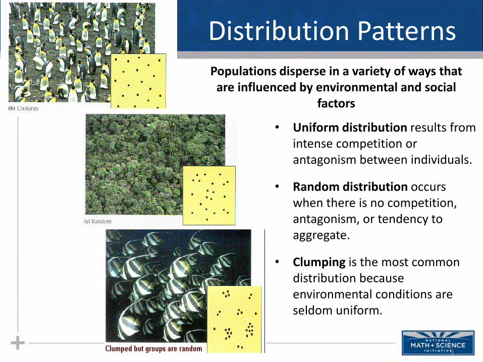
Distribution Patterns

• Uniform distribution results from intense competition or antagonism between individuals.

• Random distribution occurs when there is no competition, antagonism, or tendency to aggregate.

• Clumping is the most common distribution because environmental conditions are seldom uniform.

3

Populations disperse in a variety of ways that are influenced by environmental and social

factors

Fig. 52.1, Campbell & Reece, 6th ed.

Clumped distribution in species acts as a mechanism against predation as well as an efficient mechanism to trap or corner prey. It has been shown that larger packs of animals tend to have a greater number of successful kills.

What causes these populations of different organisms to clump together?

Population Dispersal

• Natural range expansions show the influence of dispersal on distribution

– For example, cattle egrets arrived in the Americas in the late 1800s and have expanded their distribution

5

Population Dispersal

• In rare cases, long-distance dispersal can lead to adaptive

radiation

– For example, Hawaiian silverswords are a diverse group descended from an ancestral North American tarweed

6

The Spread of the Africanized Honey Bee

When did they first arrive in the Americas?

How long did it take for them to expand their range into the US?

How can you explain their success in expanding their territory?

7

Small Geographic Range

8

Species with a Large Geographic Range

9

Moss Tetraphis

Interactions

10

11

Estimating Population SizeThe Mark-and-Recapture Technique

1. 2.

3.

Estimating Population SizeThe Mark-and-Recapture Technique

• There’s a simple formula for estimating the total population size

𝑠

𝑁=𝑥

𝑛s = Number of individuals marked and released in 1st sample

x = Number of individuals marked and released in 2nd sample

n = Total number of individuals in 2nd sample

N = Estimated population size

Rearrange to get: 𝑁 =𝑠𝑛

𝑥

12

Let’s Try an Example!

13

• Twenty individuals are captured at random and marked with a dye or tag and then are released back into the environment.

• Therefore s = # of animals marked = 20

• At a later time a second group of animals is captured at random from the population

Let’s Try an Example!

14

• Some will already be marked, say 10 individuals were marked out of 35 that were captured the second time. We now know n = 35 and x = 10

• So, apply the formula and solve for the estimated population size:

𝑁 =𝑠𝑛

𝑥=

20 35

10=

700

10= 70

Therefore, N = 70 as a population estimate

15

Which method would you use?

1. To determine the number of deer in the state of Virginia?

2. To determine the number of turkeys in a county?

3. To determine the number of dogs in your neighborhood?

4. To determine the number of feral cats in your neighborhood?

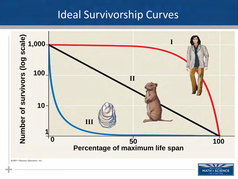
Survivorship curves

What do these graphs indicate regarding species survival rate & strategy?

0 25

1000

100

Human(type I)

Hydra(type II)

Oyster(type III)

10

1

50

Percent of maximum life span

10075

Surv

ival

per

th

ou

san

d

I. High death rate in post-reproductive years

II. Constant mortality rate throughout life span

III. Very high early mortality but the few survivors then live long (stay reproductive)

1,000

III

II

I

100

10

1

100500

Percentage of maximum life span

Nu

mb

er

of

su

rviv

ors

(lo

g s

cale

)Ideal Survivorship Curves

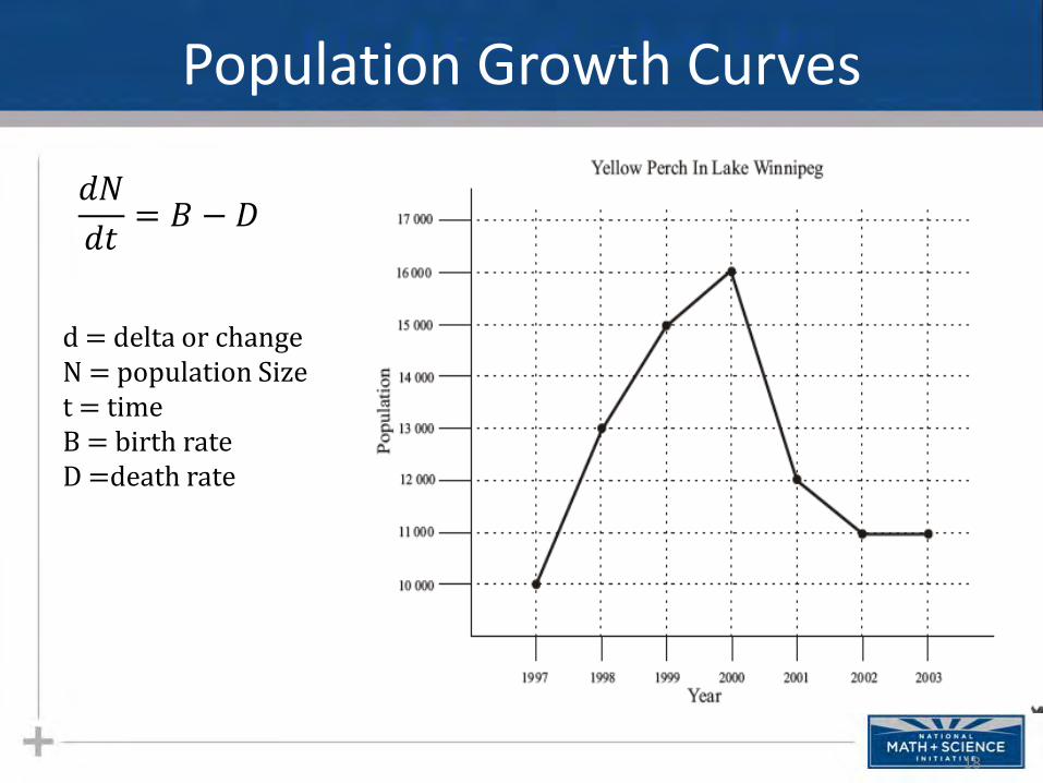
Population Growth Curves

18

d = delta or changeN = population Sizet = timeB = birth rateD =death rate

𝑑𝑁

𝑑𝑡= 𝐵 − 𝐷

Population Growth Models

Exponential model (blue)

idealized population in an unlimited environment (J-curve); can’t continue indefinitely. r-selected species (r = per capita growth rate)

𝑑𝑁

𝑑𝑡= 𝑟𝑚𝑎𝑥𝑁

Logistic model (red) considers population density on growth (S-curve), carrying capacity (K): maximum population size that a particular environment can support; K-selected species

𝑑𝑁

𝑑𝑡= 𝑟𝑚𝑎𝑥𝑁

𝐾 − 𝑁

𝐾

Exponential Growth Curves

20

d = delta or changeN = Population Sizet = timermax = maximum per

capita growth rate of population

𝒅𝑵

𝒅𝒕= 𝒓𝒎𝒂𝒙𝑵

Pop

ula

tio

n S

ize,

N

Time (hours)

Growth Rate of E. coli

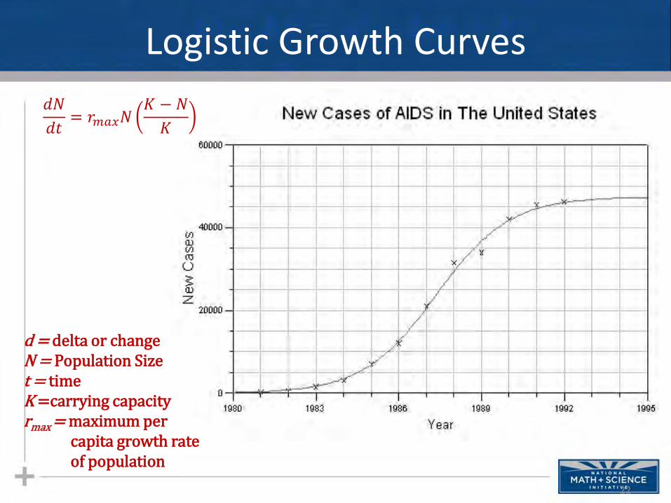
Logistic Growth Curves

21

• In the logistic population growth model, the per capita rate of increase (rmax) declines as carrying capacity (K) is reached

• The logistic model starts with the exponential model and adds an expression that reduces per capita rate of increase as N approaches K

𝑑𝑁

𝑑𝑡= 𝑟𝑚𝑎𝑥𝑁

𝐾 − 𝑁

𝐾

Logistic Growth Curves

22

d = delta or changeN = Population Sizet = timeK =carrying capacityrmax = maximum per

capita growth rate of population

𝑑𝑁

𝑑𝑡= 𝑟𝑚𝑎𝑥𝑁

𝐾 − 𝑁

𝐾

Comparison of Growth Curves

23

Growth Curve Relationship

24

Examining Logistic Population Growth

Graph the data given as it relates to a logistic curve.

Title, label and scale your graph properly.

25

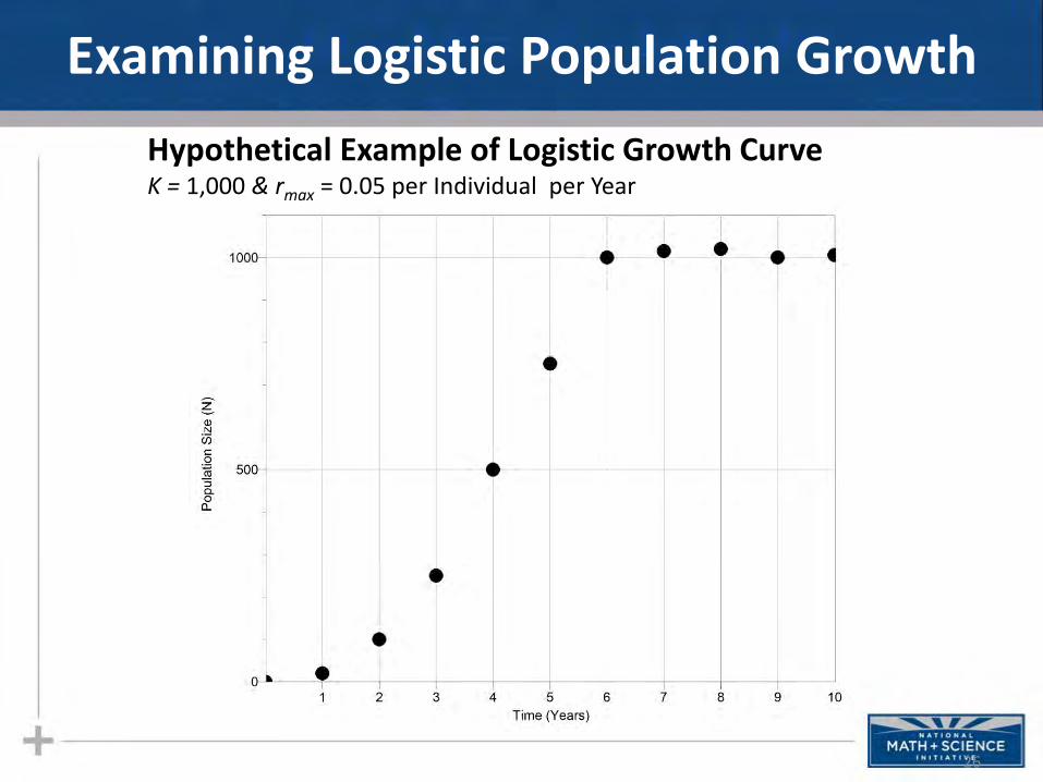
Examining Logistic Population Growth

26

Hypothetical Example of Logistic Growth Curve K = 1,000 & rmax = 0.05 per Individual per Year

Population Reproductive Strategies

• r-selected (opportunistic)

• Short maturation & lifespan

• Many (small) offspring; usually 1 (early) reproduction;

• No parental care

• High death rate

• K-selected (equilibrial)

• Long maturation & lifespan

• Few (large) offspring; usually several (late) reproductions

• Extensive parental care

• Low death rate

28

Some populations overshoot Kbefore settling down to a relatively stable density

Some populations fluctuate greatly and make it difficult to define K

How Well Do These Organisms Fit the Logistic Growth Model?

Introduced Species

• What’s the big deal?

• These species are free from predators, parasites and pathogens that limit their populations in their native habitats.

• These transplanted species disrupt their new community by preying on native organisms or outcompeting them for resources.

29

Guam: Brown Tree Snake

• The brown tree snake was accidentally introduced to Guam as a stowaway in military cargo from other parts of the South Pacific after World War II.

• Since then, 12 species of birds and 6 species of lizards the snakes ate have become extinct.

• Guam had no native snakes.

30

Dispersal of Brown Tree Snake

Predator Removal

32

Removing both limpets and urchins or removing only urchins increased seaweed cover dramatically

Predator Removal

33

Almost no seaweed grew in areas where both urchins and limpets were present (red line) ,

OR

where onlylimpets were removed (blue line)