pom - chapter 15 demand management 190111

8/4/2019 POM - Chapter 15 Demand Management 190111

http://slidepdf.com/reader/full/pom-chapter-15-demand-management-190111 1/40

1

POM/sem2/divB/AA/Ch15 1



2

©The McGraw-Hill Companies, Inc., 2006 McGraw-Hill/Irwin

Chapter 15

Demand Management



3


•Demand Management•Qualitative Forecasting

Methods•Simple & Weighted Moving

Average Forecasts•Exponential Smoothing•Simple Linear Regression•Web-Based Forecasting

OBJECTIVES



4


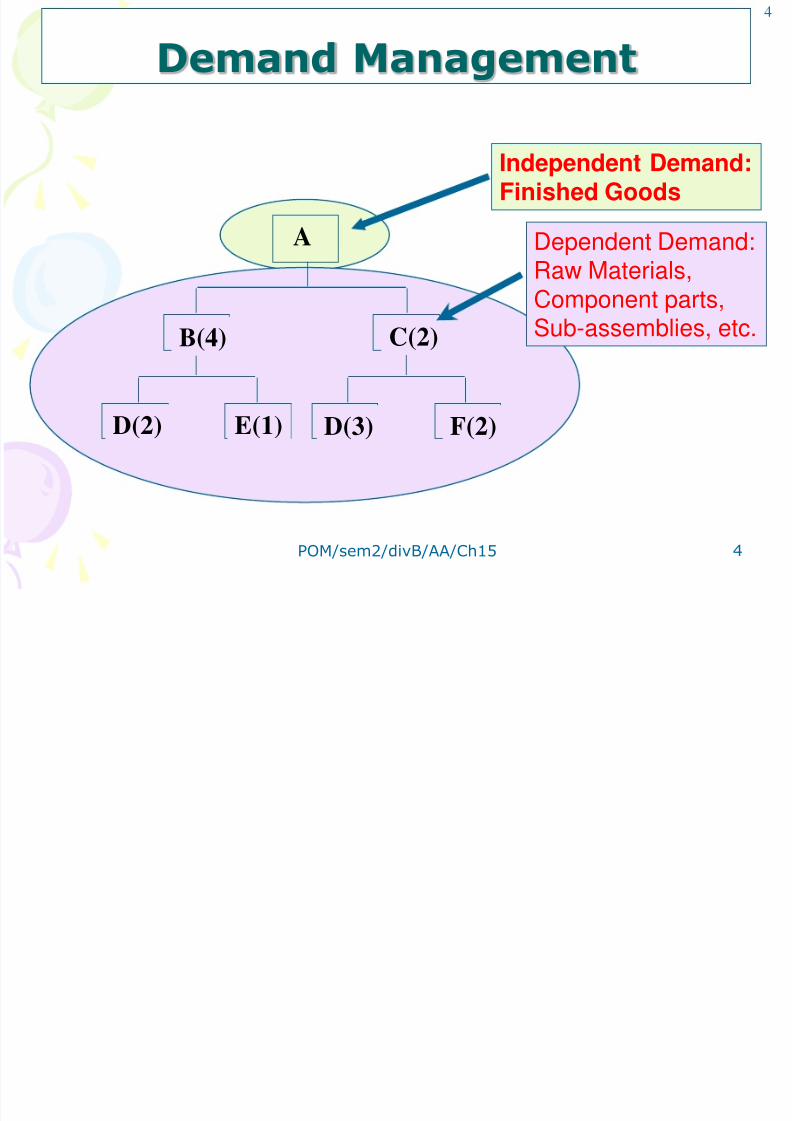
Demand Management

A

B(4) C(2)

D(2) E(1) D(3) F(2)

Dependent Demand:

Raw Materials,Component parts,Sub-assemblies, etc.

Independent Demand:Finished Goods



5


Independent Demand:What a firm can do to manage it?

• Can take an active role toinfluence demand

• Can take a passive role andsimply respond to demand



6


Types of Forecasts

• Qualitative (Judgmental)

•

Quantitative– Time Series Analysis

– Causal Relationships

– Simulation



7


Components of Demand

•Average demand for a periodof time

•Trend

•Seasonal element

•Cyclical elements

•Random variation•Autocorrelation



8


Finding Components of Demand

1 2 3 4

x

x xx

xx

x xx

xx x x x

xxxxxx x x

xx

x x xx

xx

xx

x

xx

xx

xx

x

xx

xx

x

x

x

Year

S a l e s

Seasonalvariation

Linear

Trend



9


Qualitative Methods

Grass Roots

Market Research

Panel Consensus

Executive Judgment

Historical analogy

Delphi Method

Qualitative

Methods



10


Delphi Method

l. Choose the experts to participaterepresenting a variety of knowledgeablepeople in different areas

2. Through a questionnaire (or E-mail), obtainforecasts (and any premises or qualifications

for the forecasts) from all participants3. Summarize the results and redistribute them

to the participants along with appropriatenew questions

4. Summarize again, refining forecasts andconditions, and again develop new questions

5. Repeat Step 4 as necessary and distributethe final results to all participants



11


Time Series Analysis

•

Time series forecasting modelstry to predict the future based onpast data

•

You can pick models based on:1. Time horizon to forecast

2. Data availability

3. Accuracy required

4. Size of forecasting budget

5. Availability of qualified personnel

12



12


Simple Moving Average Formula

F = A + A + A +...+An

tt -1 t-2 t-3 t-n

• The simple moving average model assumes

an average is a good estimator of futurebehavior

• The formula for the simple moving averageis:

Ft = Forecast for the coming period

N = Number of periods to be averagedA t-1 = Actual occurrence in the past period for up to “n”

periods

13



13


Simple Moving Average Problem (1)

Week Demand

1 650

2 678

3 7204 785

5 859

6 920

7 850

8 7589 892

10 920

11 789

12 844

F = A + A + A +...+An

t t -1 t-2 t-3 t-n

Question: What are the 3-week and 6-week

moving averageforecasts for demand?

Assume you only have 3weeks and 6 weeks of

actual demand data forthe respective forecasts

14



Week Demand 3-Week 6-Week

1 650

2 678

3 720

4 785 682.67

5 859 727.676 920 788.00

7 850 854.67 768.67

8 758 876.33 802.00

9 892 842.67 815.33

10 920 833.33 844.00

11 789 856.67 866.50

12 844 867.00 854.83

F4=(650+678+720)/3

=682.67

F7=(650+678+720

+785+859+920)/6

=768.67

Calculating the moving averages gives us:

©The McGraw-Hill Companies, Inc., 2004

14

15



15


500

600

700

800

900

1000

1 2 3 4 5 6 7 8 9 10 11 12

Week

D e m a n d Demand

3-Week

6-Week

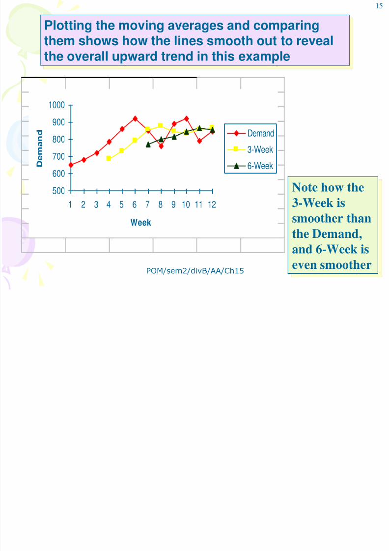
Plotting the moving averages and comparingthem shows how the lines smooth out to revealthe overall upward trend in this example

Note how the

3-Week issmoother than

the Demand,

and 6-Week is

even smoother



17



17


Simple Moving Average Problem(2) Solution

Week Demand 3-Week 5-Week

1 820

2 7753 680

4 655 758.33

5 620 703.33

6 600 651.67 710.00

7 575 625.00 666.00

F4=(820+775+680)/3

=758.33F6=(820+775+680

+655+620)/5

=710.00

18



18


Weighted Moving AverageFormula

F = w A + w A + w A + ...+ w At 1 t -1 2 t -2 3 t -3 n t - n

w =1ii=1

n

While the moving average formula implies an equalweight being placed on each value that is being averaged,

the weighted moving average permits an unequal

weighting on prior time periods

wt = weight given to time period “t”

occurrence (weights must add to one)

The formula for the moving average is:

19



19


Weighted Moving Average Problem(1) Data

Weights:t-1 .5

t-2 .3

t-3 .2

Week Demand1 650

2 678

3 720

4

Question: Given the weekly demand and weights, what is

the forecast for the 4th period or Week 4?

Note that the weights place more emphasis on the

most recent data, that is time period “t-1”

20



20


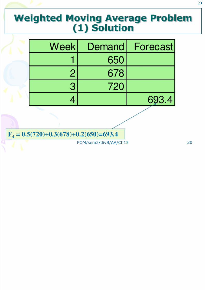
Weighted Moving Average Problem(1) Solution

Week Demand Forecast

1 650

2 6783 720

4 693.4

F4 = 0.5(720)+0.3(678)+0.2(650)=693.4



22



22


Weighted Moving Average Problem(2) Solution

Week Demand Forecast

1 820

2 775

3 680

4 655

5 672

F5 = (0.1)(755)+(0.2)(680)+(0.7)(655)= 672



24



24


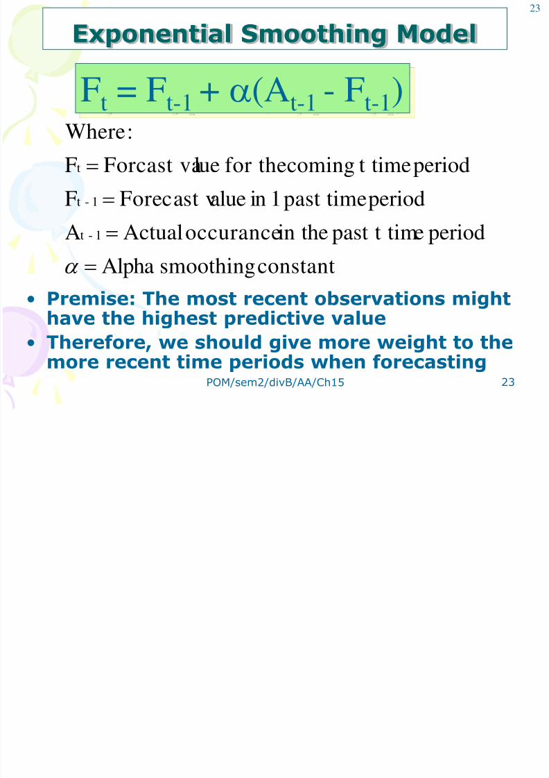
Exponential Smoothing Problem (1) Data

Week Demand

1 820

2 775

3 6804 655

5 750

6 802

7 7988 689

9 775

10

Question: Given theweekly demand data,what are theexponential

smoothing forecastsfor periods 2-10using a=0.10 anda=0.60?

Assume F1=D1

25



25


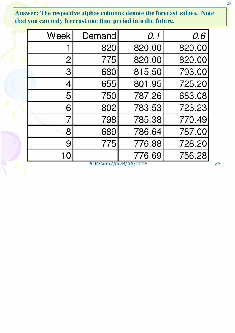
Week Demand 0.1 0.6

1 820 820.00 820.00

2 775 820.00 820.00

3 680 815.50 793.00

4 655 801.95 725.205 750 787.26 683.08

6 802 783.53 723.23

7 798 785.38 770.498 689 786.64 787.00

9 775 776.88 728.20

10 776.69 756.28

Answer: The respective alphas columns denote the forecast values. Note

that you can only forecast one time period into the future.

26




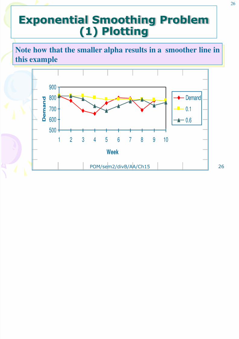
Exponential Smoothing Problem(1) Plotting

500

600

700

800

900

1 2 3 4 5 6 7 8 9 10

Week

D e m a n d Demand

0.1

0.6

Note how that the smaller alpha results in a smoother line in

this example

27




Exponential Smoothing Problem

(2) Data

Question: What are the

exponential smoothing

forecasts for periods 2-5

using a =0.5?

Assume F1=D1

Week Demand

1 8202 775

3 680

4 6555

28




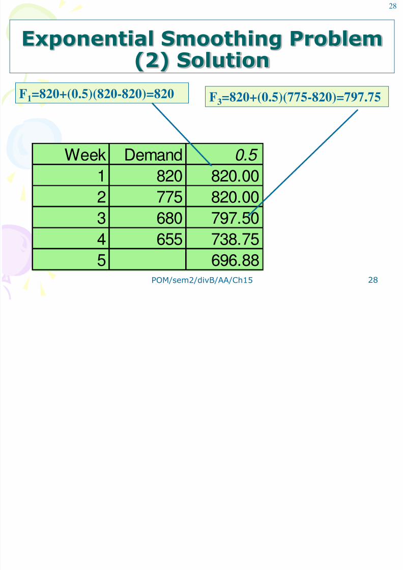
Exponential Smoothing Problem(2) Solution

Week Demand 0.5

1 820 820.00

2 775 820.00

3 680 797.50

4 655 738.75

5 696.88

F1=820+(0.5)(820-820)=820 F3=820+(0.5)(775-820)=797.75

29




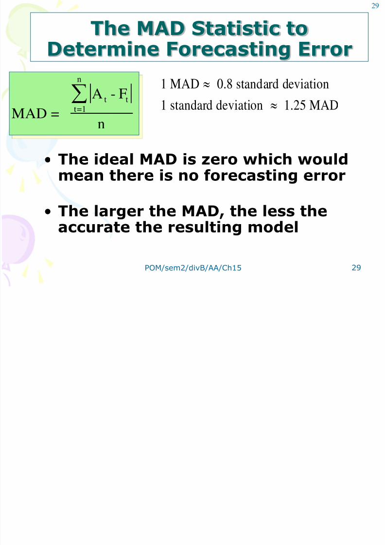
The MAD Statistic toDetermine Forecasting Error

MAD =

A - F

n

t tt=1

n

1 MAD 0.8 standard deviation

1 standard deviation 1.25 MAD

• The ideal MAD is zero which wouldmean there is no forecasting error

• The larger the MAD, the less theaccurate the resulting model

30




MAD Problem Data

Month Sales Forecast 1 220 n/a

2 250 255

3 210 205

4 300 320

5 325 315

Question: What is the MAD value given

the forecast values in the table below?

31

MAD P bl S l i




MAD Problem Solution

MAD =

A - F

n=

40

4= 10

t tt=1

n

Month Sales Forecast Abs Error

1 220 n/a

2 250 255 5

3 210 205 5

4 300 320 20

5 325 315 10

40

Note that by itself, the MADonly lets us know the mean

error in a set of forecasts

32




Tracking Signal Formula

•

The Tracking Signal or TS is a measure thatindicates whether the forecast average iskeeping pace with any genuine upward ordownward changes in demand.

• Depending on the number of MAD’s

selected, the TS can be used like a qualitycontrol chart indicating when the model isgenerating too much error in its forecasts.

• The TS formula is:

TS =RSFE

MAD=

Running sum of forecast errors

Mean absolute deviation

33




Simple Linear Regression Model

Yt = a + bx

0 1 2 3 4 5 x (Time)

YThe simple linear regression

model seeks to fit a line

through various data over

time

Is the linear regression model

a

Yt is the regressed forecast value or dependent variable inthe model, a is the intercept value of the the regressionline, and b is similar to the slope of the regression line.

However, since it is calculated with the variability of thedata in mind, its formulation is not as straight forward asour usual notion of slope.

34




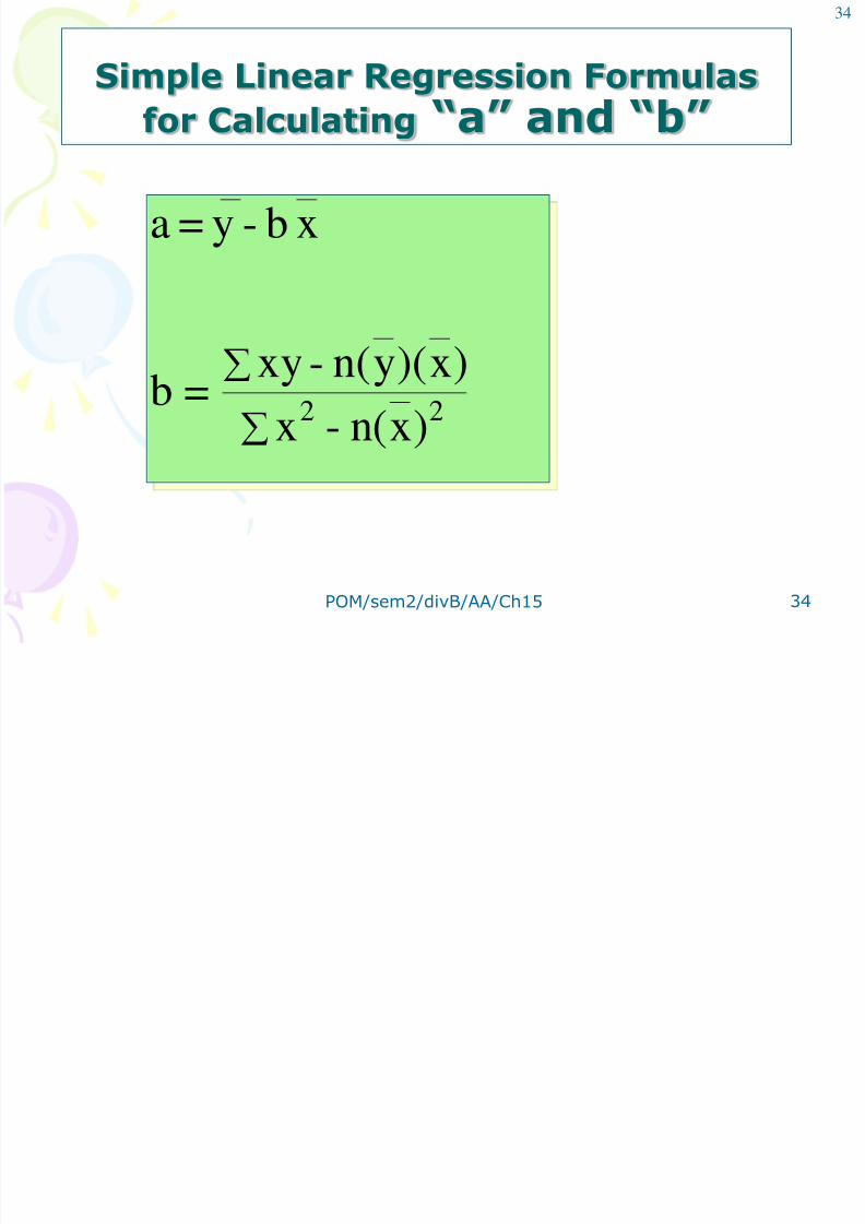
Simple Linear Regression Formulas

for Calculating “a” and “b”

a = y - b x

b =xy - n(y)(x)

x - n(x2 2

)

35




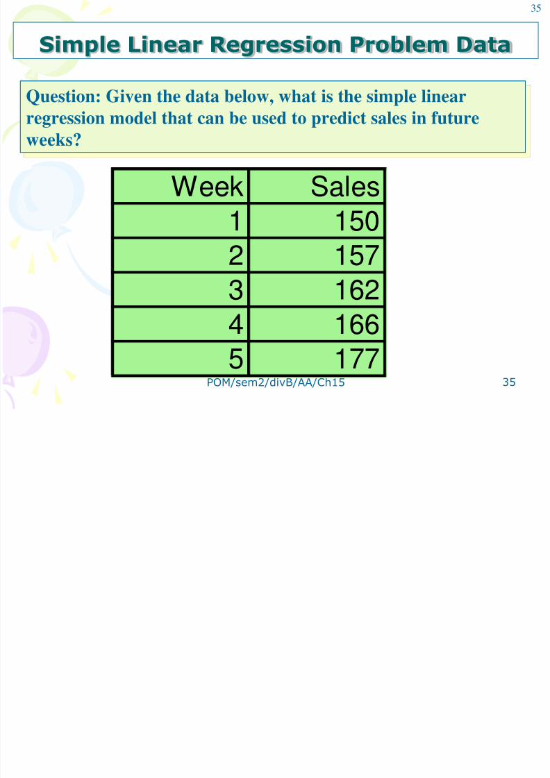
Simple Linear Regression Problem Data

Week Sales1 150

2 157

3 1624 166

5 177

Question: Given the data below, what is the simple linearregression model that can be used to predict sales in future

weeks?

36



Week Week*Week Sales Week*Sales

1 1 150 1502 4 157 314

3 9 162 486

4 16 166 664

5 25 177 885

3 55 162.4 2499

Average Sum Average Sum

b = xy - n(y)(x)x - n(x

= 2499 - 5(162.4)(3) =

a = y - bx = 162.4 - (6.3)(3) =

2 2

) ( )55 5 96310

6.3

143.5

Answer: First, using the linear regression formulas, wecan compute “a” and “b”

37



Yt = 143.5 + 6.3x

180

Perio

d

135140145150155

160165

170175

1 2 3 4 5

S a l e s Sales

Forecast

The resulting regression model

is:

Now if we plot the regression generated forecasts against the

actual sales we obtain the following chart:

38




Web-Based Forecasting: CPFR

• Collaborative Planning, Forecasting, andReplenishment (CPFR) a Web-based tool usedto coordinate demand forecasting, productionand purchase planning, and inventoryreplenishment between supply chain tradingpartners.

• Used to integrate the multi-tier or n-Tier supplychain, including manufacturers, distributors andretailers.

• CPFR’s objective is to exchange selectedinternal information to provide for a reliable,

longer term future views of demand in thesupply chain.• CPFR uses a cyclic and iterative approach to

derive consensus forecasts.

39




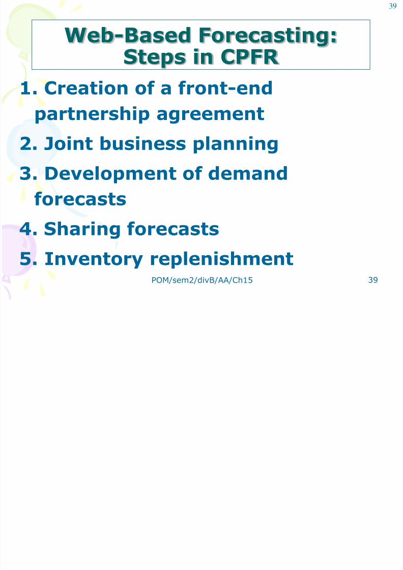
Web-Based Forecasting:Steps in CPFR

1. Creation of a front-end

partnership agreement

2. Joint business planning

3. Development of demand

forecasts

4. Sharing forecasts

5. Inventory replenishment

40



End of Chapter 15

pom - chapter 15 demand management 190111

Documents