polynomially solvable cases of hypergraph …polynomially solvable cases of hypergraph transversal...

Polynomially Solvable Cases of HypergraphTransversal and Related Problems

Imran Rauf

Thesis for obtaining the title of Doctor of Engineering

of the Faculties of Natural Sciences and Technology

of Saarland University

Saarbrucken, Germany, Oct 2011

Dean: Prof. Dr. Holger Hermanns

Faculty of Mathematics and Computer Science

Saarland University

Saarbrucken, Germany

Colloquium: 25.10.2011

Examination Board

Chair: Prof. Dr. Raimund Seidel

Reviewers: Prof. Dr. Kurt Mehlhorn

Prof. Dr. Endre Boros

Supervisor: Dr. Khaled Elbassioni

Research Assistant: Dr. Tobias Friedrich

Abstract

This thesis is mainly concerned with the hypergraph transversal problem, which asks

to generate all minimal transversals of a given hypergraph. While the current best up-

per bound on the complexity of the problem is quasi-polynomial in the combined input

and output sizes, it is shown to be solvable in output polynomial time for a number

of hypergraph classes. We extend this polynomial frontier to the hypergraphs induced

by hyperplanes and constant-sided polytopes in fixed dimension Rd and hypergraphs

for which every minimal transversal and hyperedge intersection is bounded. We also

show the problem to be fixed parameter tractable with respect to the minimum integer

k such that the input hypergraph is k-degenerate, and also with respect to its maximum

complementary degree. Whereas we improve the known bounds when the parameter

is the maximum degree of a hypergraph.

We also study the readability of a monotone Boolean function which is defined as

the minimum integer r such that it can be represented by a ∨-∧-formula with every

variable occurrence is bounded by r. We prove that it is NP-hard to approximate the

readability of even a depth three Boolean formula. We also give tight sublinear upper

bounds on the readability of a monotone Boolean function given in CNF (or DNF)

form, parameterized by the number of terms in the CNF and the maximum number of

variables in the intersection of any constant number of terms. For interval DNF’s we

give much tighter logarithmic bounds on the readability.

Finally, we discuss an implementation of a quasi-polynomial algorithm for the hy-

pergraph transversal problem that runs in polynomial space. We found our implemen-

tation to be competitive with all but one previous implementation on various datasets.

Kurzfassung

Diese Dissertation behandelt hauptsachlich das Transversalhypergraphen-Problem:

gegeben ein Hypergraph, generiere alle seine minimalen Transversalen. Obwohl die

bisher beste obere Schranke fur die Komplexitat dieses Problems quasi-polynomiell

in der Große der Ein- und Ausgabe ist, sind fur viele Klassen von Hypergraphen

output-polynomielle Losungen bekannt. Wir zeigen fr zwei weitere Klassen von Hy-

pergraphen, dass sie output-polynomielle Losungen besitzen. Zum einen sind dies

Hypergraphen, die durch Hyperebenen und Polytope mit konstanter Seitenzahl im Rd

fur eine feste Dimension d induziert werden; zum anderen sind dies Hypergraphen,

fur die die Große der Schnittmenge jedes Transversalen und jeder Hyperkante beschrankt

ist. Desweiteren zeigen wir, dass das Problem fixed-parameter tractable ist, wenn als

Parameter der maximale inverse Knotengrad des eingegebenen Hypergraphen gewahlt

wird oder der Parameter k die kleinste naturliche Zahl ist, fur die der eingegebene Hy-

pergraph k-degeneriert ist. Wir verbessern die bekannten fixed-parameter Ergebnisse

fur den Parameter des maximalen Knotengrads des eingegebenen Hypergraphen.

Außerdem untersuchen wir die readability von monotonen Booleschen Funktio-

nen. Diese ist als kleinste naturliche Zahl r definiert, so dass die Funktion als ∨-∧-

Formel reprasentiert werden kann, in der jede Variable hochstens r-mal vorkommt.

Wir beweisen, dass die Approximation der readability schon fur Boolesche Formeln

der Tiefe 3 NP-hart ist. Daruberhinaus geben wir scharfe sublineare untere Schranken

fur die readability monotoner Boolescher Funktionen an, die in KNF-Form (oder DNF-

Form) gegeben sind, wenn uber die Anzahl der Terme der KNF und die maximale An-

zahl an Variablen im Durchschnitt einer konstanten Anzahl von Termen parametrisiert

wird. Fur intervall-DNF geben wir noch scharfere logarithmische Schranken fur die

readability an.

Schließlich behandeln wir fur das Transversalhypergraphen-Problem noch die Im-

plementation eines quasi-polynomiellen Algorithmus, der mit polynomiellen Platzbe-

darf auskommt. Auf verschiedenen Datensatzen ist unsere Implementation zu allen

vorherigen Implementationen (außer einer) konkurrenzfahig.

Acknowledgements

This work would have been impossible without the much needed encouragement

and energetic input from my advisor Khaled Elbassioni throughout its development

and completion, for which I am really grateful to him. I am indebted to Kurt Mehlhorn,

the director of Algorithm and Complexity group at the Max Planck Institute of Com-

puter Science (MPII), for giving me chance to pursue PhD in his excellent group, where

he is instrumental in maintaining a great atmosphere for research and also provides a

role model for younger members of the group. I am also grateful to Ulrich Meyer and

Stefan Funke for guiding me in the earlier phase of my PhD and Prof. Endre Boros

for agreeing to examine my thesis. I was fortunate to receive the generous stipend

awarded by International Max Planck Research School for Computer Science which

supported me throughout my time at MPII. I would like to thank my coauthors Khaled

Elbassioni, Stefan Funke, Kaz Makino, Matthias Hagen and Saurabh Ray. Matthias also

did a great favor by translating the abstract into German.

My colleagues and friends helped me immensely in some way or another while I

was working on this thesis. Here I would like to acknowledge some names that come

to mind now: Tobias and Evangelia for being great officemates; Deepak, Hans, Saurabh

and Vikram for being good friends and inspiring colleagues; Amir, Anuj, Kara, Awais,

Habeeb and Sikander for many fun activities we did together; and Safdar, Sohail, Atif,

Mujtaba, Usman, Yasir, Jamal, Naveed, Shahid, Khurram, Hameed and Fawad for

countless political/religious discussions while enjoying delicious Pakistani food to-

gether.

Finally, I cannot express my gratitude enough for my parents Abdul Rauf and

Mussarat-un-Nissa, and my siblings Adnan, Saba, Salman and Masoom. It was my

elder brother Adnan who introduced me to Computer Science in the first place. This

thesis is dedicated to my wife Saeeda and our sweet daughter Manal.

iii

Contents

Abstract i

Kurzfassung ii

Acknowledgements iii

1 Introduction 1

1.1 Previous Work . . . . . . . . . . . . . . . . . . . . . . . . . . . . . . . . . . 1

1.2 Summary and Outline of the Thesis . . . . . . . . . . . . . . . . . . . . . 2

2 Preliminaries 5

2.1 Background and Notation . . . . . . . . . . . . . . . . . . . . . . . . . . . 5

2.2 Properties of the Transversal Hypergraph . . . . . . . . . . . . . . . . . . 8

2.3 Hypergraph Transversal Problem . . . . . . . . . . . . . . . . . . . . . . . 10

2.4 Enumeration Techniques . . . . . . . . . . . . . . . . . . . . . . . . . . . . 12

2.4.1 Berge Multiplication . . . . . . . . . . . . . . . . . . . . . . . . . . 12

2.4.1.1 Dualizing Small Instances . . . . . . . . . . . . . . . . . 14

2.4.2 Backtracking Method . . . . . . . . . . . . . . . . . . . . . . . . . 14

2.4.3 Incremental Method . . . . . . . . . . . . . . . . . . . . . . . . . . 15

2.4.4 Divide and Conquer . . . . . . . . . . . . . . . . . . . . . . . . . . 17

2.4.5 Full Cover Decompositions . . . . . . . . . . . . . . . . . . . . . . 18

2.5 Related Problems . . . . . . . . . . . . . . . . . . . . . . . . . . . . . . . . 21

2.5.1 Dualization of Monotone Boolean Functions . . . . . . . . . . . . 21

iv

2.5.2 Frequent Sets in Databases . . . . . . . . . . . . . . . . . . . . . . 22

3 Fixed Parameter Algorithms 24

3.1 Introduction . . . . . . . . . . . . . . . . . . . . . . . . . . . . . . . . . . . 24

3.2 Number of Edges as Parameter . . . . . . . . . . . . . . . . . . . . . . . . 25

3.3 Hypergraph Degeneracy as Parameter . . . . . . . . . . . . . . . . . . . . 27

3.4 Vertex complementary degree as parameter . . . . . . . . . . . . . . . . . 28

3.5 Results Based on the Apriori Technique . . . . . . . . . . . . . . . . . . . 28

4 r-Exact Hypergraphs 31

4.1 Introduction . . . . . . . . . . . . . . . . . . . . . . . . . . . . . . . . . . . 31

4.2 Applications in geometry . . . . . . . . . . . . . . . . . . . . . . . . . . . 33

4.2.1 Circular-arc hypergraphs . . . . . . . . . . . . . . . . . . . . . . . 33

4.2.2 Translates of cones in R2 . . . . . . . . . . . . . . . . . . . . . . . . 35

4.2.3 Stabbing fat objects in Rd . . . . . . . . . . . . . . . . . . . . . . . 36

4.3 Dualization of r-exact hypergraphs . . . . . . . . . . . . . . . . . . . . . . 37

4.3.1 Decompositions . . . . . . . . . . . . . . . . . . . . . . . . . . . . . 38

4.3.2 Algorithm . . . . . . . . . . . . . . . . . . . . . . . . . . . . . . . . 40

4.4 Conclusions . . . . . . . . . . . . . . . . . . . . . . . . . . . . . . . . . . . 41

5 Geometric Hypergraphs 43

5.1 Introduction . . . . . . . . . . . . . . . . . . . . . . . . . . . . . . . . . . . 43

5.2 First Approach: Using Elementary Techniques . . . . . . . . . . . . . . . 44

5.2.1 A Framework for Computing Transversal Hypergraphs . . . . . 45

5.2.2 Points and Hyper-rectangles in Rd . . . . . . . . . . . . . . . . . . 47

5.2.3 Stabbing Connected Objects in Rd . . . . . . . . . . . . . . . . . . 48

5.3 Second Approach: Using Cuttings and Simplicial Partitions . . . . . . . 51

5.3.1 Introduction . . . . . . . . . . . . . . . . . . . . . . . . . . . . . . . 51

5.3.2 Balanced Subdivisions . . . . . . . . . . . . . . . . . . . . . . . . . 52

5.3.3 The Enumeration Algorithm . . . . . . . . . . . . . . . . . . . . . 55

v

5.3.4 Application - Infrequent pointsets . . . . . . . . . . . . . . . . . . 59

5.4 Enumerating Minimal Hitting Sets of Half-Planes with Polynomial Delay 60

5.4.1 Backtracking Method . . . . . . . . . . . . . . . . . . . . . . . . . 62

5.4.2 Checking the Sub-Transversal Criterion . . . . . . . . . . . . . . . 63

5.5 Conclusions . . . . . . . . . . . . . . . . . . . . . . . . . . . . . . . . . . . 64

6 Readability 65

6.1 Introduction . . . . . . . . . . . . . . . . . . . . . . . . . . . . . . . . . . . 66

6.2 On Generalization of Read-Once Functions . . . . . . . . . . . . . . . . . 68

6.3 Upper Bounds . . . . . . . . . . . . . . . . . . . . . . . . . . . . . . . . . . 69

6.3.1 Interval DNF . . . . . . . . . . . . . . . . . . . . . . . . . . . . . . 69

6.3.2 (p, q)-intersecting DNF . . . . . . . . . . . . . . . . . . . . . . . . . 71

6.3.3 k-DNF . . . . . . . . . . . . . . . . . . . . . . . . . . . . . . . . . . 74

6.4 Hardness and Inapproximability . . . . . . . . . . . . . . . . . . . . . . . 76

6.5 Conclusions . . . . . . . . . . . . . . . . . . . . . . . . . . . . . . . . . . . 79

7 Algorithm Engineering 81

7.1 The Basic Algorithm . . . . . . . . . . . . . . . . . . . . . . . . . . . . . . 81

7.2 Implementation with Polynomial Space . . . . . . . . . . . . . . . . . . . 83

7.3 Results . . . . . . . . . . . . . . . . . . . . . . . . . . . . . . . . . . . . . . 86

7.4 Conclusions . . . . . . . . . . . . . . . . . . . . . . . . . . . . . . . . . . . 90

List of Algorithms 91

List of Figures 92

List of Tables 93

Bibliography 94

vi

Chapter 1

Introduction

Monotone enumeration problems, which call for finding all objects or configurations

satisfying a certain monotone property, are often captured by the hypergraph transversal

problem. Although transversal hypergraphs have been studied before by mathemati-

cians, Johnson, Papadimitriou and Yannakakis [JPY88] first proposed it as a compu-

tation problem. Currently, the fastest known algorithm [FK96] for solving the hyper-

graph transversal problem runs in time quasi-polynomial in the combined input and

output size. In this chapter we give a brief overview of the problem. We then give a

summary of the work presented in the thesis.

1.1 Previous Work

The hypergraph transversal problem asks to generate all minimal transversals (hitting-sets)

of a given hypergraph. The family of all minimal transversals, which itself is a hyper-

graph, is called transversal hypergraph. This problem has received considerable atten-

tion in the literature (see, e. g., [BI95, EG95, EGM03, Got04, Lov92, Pap97]), since it

is known to be polynomially or quasi-polynomially equivalent with many problems

in various areas, such as artificial intelligence (e. g., [EG95, KPS93]), database theory

(e. g., [MR86]), distributed systems (e. g., [GMB85, IK93]), machine learning and data

mining (e. g., [AB92, BGKM02, GMKT97]), mathematical programming (e. g., [BEG+02,

1

Kha00]), matroid theory (e. g., [KBE+05]), and reliability theory (e. g., [Col87, Ram90])

to name a few.

As the number of minimal transversals of a hypergraph can be exponential in

the size of the input hypergraph, one can only hope for an algorithm whose effi-

ciency is measured in terms of combined input and output sizes. The currently fastest

known algorithm [FK96] for solving the hypergraph transversal problem runs in quasi-

polynomial time N o(logN), where N is the combined input and output size. Several

quasi-polynomial time algorithms with some other desirable properties also exist. A

parallel algorithm that runs in polylogarithmic time using quasi-polynomial number

of processors is recently given in [Elb08, BM09]. Other algorithms that match the

current best quasi-polynomial bound and run in polynomial space are presented in

[Tam00, Elb08]. An algorithm that use only multiplication is shown to achieve quasi-

polynomial time in [Elb06]. Yet another quasi-polynomial time algorithm for a variant

of the hypergraph transversal problem is analyzed with respect to its average case com-

plexity in [GK04]. The decision version of the problem is known to be solvable with

limited nondeterminism [KS03], i. e., by nondeterministic polynomial time algorithm

that makes only polylogarithmic number of guesses.

While it is still open whether the problem can be solved in output polynomial time

for arbitrary hypergraphs, output polynomial time algorithms exist for several classes

of hypergraphs, e. g., hypergraphs of bounded edge-size [BEGK04, EG95], of bounded

degree [DMP99, EGM03], of bounded-edge intersections [BEGK04], of bounded con-

formality [BEGK04], of bounded treewidth [EGM03], of bounded latency [MI97], and

read-once (exact) hypergraphs [Eit94].

1.2 Summary and Outline of the Thesis

The basic definitions and notations are introduced in Chapter 2, which also briefly

presents the results about the hypergraph transversal problem relevant to this thesis.

2

CHAPTER 1. INTRODUCTION 3

We then proceed in the following three chapters with showing the output polynomial

time solvability of the hypergraph transversal problem for the following classes of hy-

pergraphs.

Fixed Parameter Tractability (Chapter 3): We present FPT algorithms for the hypergraph

transversal problem with the number of edges of the hypergraphs, the minimum in-

teger k such that the input hypergraph is k-degenerate, and the vertex complemen-

tary degree as our parameters. Moreover, we also get FPT results for the hypergraph

transversal problem as well as the related problems of generating all maximal inde-

pendent sets of a hypergraph and all maximal frequent sets where parameters bound

the intersections or unions of edges.

r-Exact Hypergraphs (Chapter 4): We call a hypergraphH is r-exact for a positive integer

r, if any minimal transversal of H intersects any hyperedge of H in at most r vertices.

This class includes several interesting examples from geometry, e.g., circular-arc hy-

pergraphs (r = 2), hypergraphs defined by sets of axis-parallel lines stabbing a given

set of α-fat objects (r = 4α), and hypergraphs defined by sets of points contained in

translates of a given cone in the plane (r = 2). For constant r, we give a polynomial-

time algorithm to decide for a pair of r-exact hypergraphs, if one is the transversal

hypergraph of the other. This result implies that minimal hitting sets for the above

geometric hypergraphs can be generated in output polynomial time.

Geometric Hypergraphs (Chapter 5): For hypergraphs induced by intersections of a fam-

ily of geometrical objects by another, we introduce two general frameworks to gen-

erate the transversal hypergraph. The first approach use only elementary techniques,

and gives a polynomial-time algorithm for the problem of hitting hyper-rectangles by

points, and stabbing connected objects by axis-parallel hyperplanes, both in Rd for

a fixed d. Overcoming the limitations of the first approach, we give another tech-

nique that use simplicial partitions and cuttings to efficiently enumerate all minimal

hitting-sets as well as minimal covers of hypergraphs defined by intersections of sets

of points with hyperplanes (and hence balls) or more generally, constant-sided poly-

topes in fixed dimension Rd. Finally, we give a polynomial delay algorithm for the

special case of hypergraphs induced by half-planes and points in R2.

In the second half of the thesis, we begin with a study of a complexity measure

for monotone Boolean functions called readability in Chapter 6. The readability of a

monotone Boolean function f : 0, 1n → 0, 1 is defined to be the minimum integer

k such that there exists an ∧-∨-formula equivalent to f in which each variable appears

at most k times. An important open problem in this area is whether there exists a

polynomial-time algorithm, which given a monotone Boolean function f , in CNF or

DNF form, checks whether f is a read-k function, for a fixed k. We answer a related

question already for k = 2 by showing that it is NP-hard to decide if a given monotone

formula represents a read-twice function. It follows also from our reduction that it

is NP-hard to approximate the readability of a given monotone Boolean function f

within a factor of O(n). We also give tight sublinear upper bounds on the readability

of a monotone Boolean function given in CNF (or DNF) form, parameterized by the

number of terms in the CNF and the maximum size in each term, or more generally

by the maximum number of variables in the intersection of any constant number of

terms. When the variables of the DNF can be ordered so that each term consists of a

set of consecutive variables, we give much tighter logarithmic bounds on readability.

Finally, we discuss an implementation of a polynomial space algorithm of Elbas-

sioni [Elb08] for the hypergraph transversal problem in Chapter 7. The distinguishing

feature of our implementation is that it requires polynomial space with the same bound

on the running time as the current best. In contrast, all of the previous implementations

either have exponential worst-case running time or need super-polynomial space. We

found our implementation to be competitive with all but one previous implementation

on various datasets.

4

Chapter 2

Preliminaries

2.1 Background and Notation

A hypergraph is a pair (V,H) where V = [n]def= 1, 2, . . . , n is a ground set and mem-

bers ofH are subsets of V , i. e.,H ⊆ 2V . Hypergraphs can be viewed as generalizations

of graphs and in that respect, elements of V and H are called vertices and hyperedges,

respectively. When the set of vertices V is clear from the context, we only refer to H

as our hypergraph for notational convenience and denote by V (H) the vertex set ofH.

We also sometimes omit the prefix hyper and refer to the the elements of H as simply

edges. A hypergraphH is called trivial whenH is empty.

A hypergraph H = H1, . . . , Hm is Sperner when for any two hyperedges Hi, Hj

of H, Hi ⊆ Hj implies i = j, i. e., when no hyperedge contains another. For any

hypergraph H ⊆ 2V , let us denote by min(H) the Sperner hypergraph we get after

deleting the inclusion-wise non-minimal hyperedges inH.

A vertex u ∈ V hits a hyperedge H ∈ H when u ∈ H . A subset of vertices X ∈ V is

called a transversal (or a hitting-set) of the hypergraph H ⊆ 2V when every hyperedge

of H is hit by some element in X , i. e., X ∩ H 6= ∅, ∀H ∈ H. A transversal is minimal

when any of its proper subsets is not a transversal. The hypergraph consisting of all

minimal transversals of H is called the transversal hypergraph of H and is denoted by

5

Hd. Note that Hd is Sperner by definition. Also, it is well known that (Hd)d = min(H)

(see Section 2.2 for a proof) and soHd is also called the dual hypergraph ofH.

Example 2.1 (Matching). Let our hypergraph beH = i, n+ i | i = 1, . . . , n, where n is

a positive integer. Then its dual hypergraph isHd = j1, j2, . . . , jn | ji ∈ i, n+ i.

Example 2.2 (Bipartite Graph Kn,n). Let H = i, n+ j | i, j = 1, . . . , n, where n is a

positive integer. Its dual hypergraph isHd = 1, 2, . . . , n , n+ 1, n+ 2, . . . , 2n.

For any subset X of V , let X denotes the compliment of X , i. e., X def= V \X . More-

over, let Hc denote the hypergraph consisting of compliments of hyperedges in H,

i. e.,Hc def= H|H ∈ H.

A subset of vertices I ∈ V is called an independent set of the hypergraph H ⊆ 2V

when I does not contain any hyperedge of H, i. e., H 6⊆ I , for all H ∈ H. It is max-

imal when any of its proper supersets is not an independent set. Note that if I is an

independent set of H then I ∩ H 6= ∅ for all H ∈ H, i. e., I is a transversal of H. In

particular, I is a minimal transversal ofH if and only if I is a maximal independent set

ofH. Consequently, the set of all maximal independent sets is equal to the hypergraph

Hdc def= (Hd)c.

For a hypergraph (V,H = H1, . . . , Hm), let us define its transposed hypergraphHt

whose vertices corresponds to hyperedges of H and every vertex u ∈ V defines a

hyperedge H | H 3 u inHt.

A hyperedge H ∈ H covers a vertex u ∈ V when H 3 u. A subset of hyperedges

H′ ⊆ H is called a covering of hypergraph (V,H) when every vertex is covered by some

hyperedge inH′, i. e.,⋃H∈H′ H = V . Note that by definition,H′ ⊆ H is a covering of V

if and only ifH′ is a transversal of the transposed hypergraphHt and so the problem of

finding all minimal coverings of H is equivalent to the problem of finding all minimal

transversals of its transposed hypergraphHt.

For any hypergraphH ⊆ 2V and a subset S ⊆ V , we use the following notations: HS

denotes the sub-hypergraph induced by the vertices in S, i. e.,HSdef= H ∈ H |H ⊆ S,

6

CHAPTER 2. PRELIMINARIES 7

and HS denotes the projection of H on S, i. e., HS def= min(H ∩ S | H ∈ H). Note that

HS is empty when S is not a hitting set ofH.

Given two hypergraphsH1 andH2 with vertex set V , denote by

H1 ∧H2def= minH1 ∪H2 |H1 ∈ H1 and H2 ∈ H2,

H1 ∨H2def= min(H1 ∪H2)

the conjunction and disjunction ofH1 andH2, respectively.

Let us denote the degree of a vertex in hypergraphH by degH(v), which is the num-

ber of hyperedges of H containing v ∈ V . Also, we sometimes write V \ v instead of

V \ v for brevity.

A hypergraph H is said to be k-Helly if for any H′ ⊆ H the following holds: if

every k hyperedges in H′ have a non-empty intersection then all edges in H′ have a

non-empty intersection.

A hypergraph is said to be k-conformal [Ber89] if any set X ⊆ V is contained in a

hyperedge of H whenever each subset of X of cardinality at most k is contained in a

hyperedge ofH. We have the following proposition.

Proposition 2.3 (cf. [Ber89]). A hypergraph H is k-Helly if and only if its transpose Ht is

k-conformal.

A hypergraph H is said to be k-degenerate [EGM02] if for every set X ⊆ V = V (H),

the minimum degree of a vertex in the induced hypergraph HX on X is most k. Let

v1 ∈ V be a vertex with minimum degree in H. Since H is k-degenerate, we know

that degH(v) ≤ k. Now consider the induced hypergraph HV \v1 on the remaining

vertices. By the definition of k-degeneracy, there exists a vertex v2 in V \ v1 such that

degree of v2 in HV \v1 is at most k. In particular a vertex with minimum degree in the

induced hypergraph satisfies this property. Consequently, we get an ordering v1, . . . , vn

of vertex set V such that for each 1 ≤ i ≤ n, the degree of vi in HV \vi,...,vn is at most

k. In fact, it can be easily shown that a hypergraph is k-degenerate if and only if there

exists such ordering of its vertices. Note that the hypergraphs in which every vertex

has degree at most k are also k-degenerate.

A hypergraph H is said to be r-exact if any minimal transversal of H intersects any

hyperedge ofH in at most r vertices.

2.2 Properties of the Transversal Hypergraph

The following lemma gives a necessary and sufficient condition for one hypergraph to

be dual of another. See, for example, [Ber89, Chapter 2, Page 44] for details.

Lemma 2.4 (Vertex-coloring lemma). Let G,H be two Sperner hypergraphs on a set V . Then

H = Gd if and only if every pair (A,B) with A,B ⊂ V,A ∪B = V,A ∩B = ∅, satisfies:

(i) there exists either an H ∈ H contained in A or a G ∈ G contained in B;

(ii) these two cases cannot happen simultaneously.

Corollary 2.5. Let G,H be two Sperner hypergraphs on a set V . Then H = Gd if and only if

G = Hd.

Proof. IndeedH = Gd if and only if every pair (A,B) satisfies (i) and (ii) with G,H; that

is every pair (B,A) satisfies (i) and (ii) withH,G; that is G = Hd.

The following is a straightforward consequence of the above corollary.

Corollary 2.6. LetH be a Sperner hypergraph. Then (Hd)d = H.

The following proposition presents some necessary conditions for the pair of hy-

pergraphs to be dual of each other.

Proposition 2.7 ([FK96]). Let G,H be two Sperner hypergraphs on a set V . IfH = Gd then

G ∩H 6= ∅ for all G ∈ G, H ∈ H, (2.1)

∪G : G ∈ G = ∪H : H ∈ H, (2.2)

max|G| : G ∈ G ≤ |H| and max|H| : H ∈ H ≤ |G|. (2.3)

8


Proof. (i) Suppose Equation (2.1) does not hold for some G ∈ G, H ∈ H. Then the pair

(H,V \H) violates the condition (ii) of Lemma 2.4.

(ii) Let i ∈ G for some G ∈ G and i 6∈ H for all H ∈ H. We show that the pair

(G \ i, (V \G) ∪ i) violates the condition (i) of Lemma 2.4. Indeed G \ i does not

contain any hyperedge of Sperner hypergraph G. Also, since every H ∈ H hits G \ i,

the set (V \ G) ∪ i does not contain any hyperedge of H. The other case when there

is j ∈ H for some H ∈ H and j 6∈ G for all G ∈ G is completely symmetric.

(iii) Let G ∈ G such that |G| > |H| then clearly G is a not minimal transversal of H

by Pigeonhole principle. The other case when there is H ∈ H such that |H| > |G| is

symmetric.

In the following we discuss properties of a single minimal transversal and its sub-

sets. Let G be a hypergraph on a set V . Observe that for every minimal transversal T

of the hypergraph G and for any v ∈ T , there is always some edge G ∈ G which requires

v, i. e., G ∩ T = v. We call such a edge a certificate edge for v in T .

A subset of vertices S ⊆ V is called a sub-transversal of G if it is contained in some

minimal transversal T of G, i. e., S ⊆ T and T ∈ Gd. Given a hypergraph G ⊆ 2V and a

subset S ⊆ V of vertices, [BGH98] gave a criterion to decide if S is a sub-transversal of

G.

To describe the sub-transversal criterion, we need a few more definitions. For a

subset S ⊆ V , and a vertex v ∈ S, let Gv(S) = G ∈ G | G ∩ S = v. A selection

of |S| hyperedges Gv ∈ Gv(S) | v ∈ S is called blocked if there exists a hyperedge

G ∈ G0def= G ∈ G : G ∩ S = ∅ such that G ⊆ ⋃v∈S Gv.

Proposition 2.8 ([BGH98]). A non-empty subset S ⊆ V is a sub-transversal for G ⊆ 2V if

and only if there is a non-blocked selection Gv ∈ Gv(S) | v ∈ S for S.

It is not hard to see that the condition in Proposition 2.8 is necessary, because we can

think of a selection as a set of tentative certificates for vertices in S, and for any blocking

selection, at least one of the certificate clearly becomes invalid when S is extended to

hit the edge which blocks the selection under consideration. So there must exists a

non-blocked selection to be able to extend S to a minimal transversal.

2.3 Hypergraph Transversal Problem

Given a hypergraph as input, the hypergraph transversal problem asks to generate its

dual. Formally, we define the problem as follows.

Input: Sperner hypergraph G.

Output: The dual hypergraph Gd.

Problem DUALIZATION

As Example 2.1 shows, the size of the dual hypergraph can be exponential in the size

of the input hypergraph. So typically enumeration problems are analyzed in terms of

both input and output sizes. More concretely, let n be the number of vertices, m be the

number of hyperedges in the input hypergraph and m′ be the number of edges in the

dual hypergraph. We say an algorithm for DUALIZATION is output polynomial when

its running time can be bounded by some polynomial in n,m and m′. Moreover, an

algorithm for DUALIZATION is incremental polynomial when it enumerates one by one

all minimal transversals of the input hypergraph such that the time it takes to output

another minimal transversal is polynomial in n,m and k, the last parameter being the

size of dual hypergraph generated so far.

The notion of incremental polynomial algorithm leads to the following problem of

deciding whether a given partial list of minimal transversals is complete for the given

hypergraph. Formally, we define the problem as follows.

10


Input: Sperner hypergraph F and a subset of its minimal transversals G ⊆ Fd.

Output: True if G = Fd, otherwise return a new transversal from Fd \ G.

Problem INCRDUAL

Finally, we define the problem of deciding whether the given two hypergraphs are

dual to each other.

Input: Sperner hypergraphs F and G.

Output: True if G = Fd, False otherwise.

Problem DUAL

It is easy to see that by making m′ + 1 calls to an algorithm for INCRDUAL, we can

generate all minimal transversals and hence a polynomial time algorithm for INCRDUAL

implies an incremental polynomial algorithm for DUALIZATION. Bioch and Ibaraki

[BI95] show the following stronger result.

Proposition 2.9. The existence of any of the the following algorithms implies all of the others.

1. An incremental polynomial time algorithm for DUALIZATION.

2. A polynomial time algorithm for INCRDUAL.

3. A polynomial time algorithm for DUAL.

An output polynomial algorithm may be too expensive for some applications and

so there is a notion of a polynomial delay algorithm in which the time to produce each

successive minimal transversal is polynomial in the size of input hypergraph only.

Therefore, the total running time of a polynomial delay algorithm to generate all min-

imal transversals would be poly(n,m) ·m′.

Clearly, the problem DUAL(G,H) is in co-NP since ifH is not the transversal hyper-

graph of G then this can be witnessed by a set X ⊆ V such that

X ∩G 6= ∅ for all G ∈ G, and X 6⊇ H for all H ∈ H. (2.4)

Intuitively, X is a transversal of G (not necessarily minimal) that does not include any

hyperedge of H. Such a set X is a witness for the non-duality of the pair (G,H). Note

that the condition (2.4) is symmetric in G andH: X ⊆ V satisfies (2.4) for the pair (G,H)

if and only if V \X satisfies (2.4) for (H,G). Also, by definition, the pair (∅, ∅) is dual.

2.4 Enumeration Techniques

Is this section, we review some techniques from the literature to solve the hypergraph

transversal problem. We also present simple sub-routines in Section 2.4.1.1 which will

be used to solve small instances confronted later as base-cases in more sophisticated

algorithms.

2.4.1 Berge Multiplication

The following proposition is elementary and follows from the basic definitions.

Proposition 2.10. Given hypergraphsH1, . . . ,Hk ⊆ 2V ,

(H1 ∨ · · · ∨ Hk)d = Hd

1 ∧ · · · ∧ Hdk.

Proof. Let T be a minimal transversal ofH =∨i∈[k]Hi and let Ti = T ∩V (Hi) for i ∈ [k].

Clearly Ti is a transversal of Hi which is not necessarily minimal. Let T ′i be a minimal

transversal of Hi contained in Ti and let T ′ =⋃i∈[k] T

′i . We show that T ′ = T and so

T ∈ ∧i∈kHdi . Indeed, the existence of a vertex v ∈ T \ T ′ contradicts the assumption

that T is a minimal transversal ofH.

12


To see the other direction, let T be a set in∧i∈kHd

i . By definition T =⋃i∈[k] Ti,

where Ti ∈ Hdi for i ∈ [k] and there is no T ′ ⊂ T with T ′ =

⋃i∈[k] T

′i , where T ′i ∈ Hd

i for

i ∈ [k]. This implies that T is a minimal transversal ofH =∨i∈[k]Hi since the existence

of smaller transversal T ′′ ⊂ T of H would yield a smaller transversal of Hi for some

i ∈ [k].

Based on Proposition 2.10 we can find all minimal transversals of a given hyper-

graph by processing its edges one by one and computing all of the minimal transver-

sal of the partial hypergraph read so far. The algorithm which is attributed to Berge

[Ber89] works similar to the multiplication of algebraic expressions and hence is some-

times called Berge Multiplication in the literature.

Algorithm 1 Berge MultiplicationInput: A hypergraphH = H1, . . . , HmOutput: The dual hypergraphHd

1: X := ∅2: for i = 1, . . . ,m do3: X := X ∧ u |u ∈ Hi4: return X

The correctness of Algorithm 1 follows from Proposition 2.10 and the the invariant

that X is the transversal hypergraph of H1, . . . , Hi after every ith iteration for i =

1, . . . ,m and hence the hypergraph returned by the procedure is indeed the transversal

hypergraph of the input hypergraph H. To analyze the running time, let Γ be the

maximum size of the intermediate hypergraph X in Step 3 of Algorithm 1. Then its

running time can be bounded by O(mnΓ minm,Γ) [BEM10].

The drawback of this otherwise simple approach is that it does not in general yield

an output polynomial algorithm. To see this, consider the hypergraph in Example 2.2

given as input to Algorithm 1. If the algorithm first multiplies the n edges of the form

i, n+ i | i = 1, . . . , n, then the size of intermediate hypergraph X in Algorithm 1 is

exponential in the input plus output sizes, whereas there are only two distinct minimal

transversals of the complete hypergraph.

The above example illustrates that Berge multiplication is sensitive to the order in

which it processes hyperedges of the input hypergraph. This raises the natural ques-

tion whether there always exists an ordering in which it is output polynomial. The

answer turns out to be No as shown by Takata [Tak07] which gives a family of hy-

pergraphs for which Berge multiplication is not output polynomial for every possible

ordering of their hyperedges. On the other hand, sub-exponential bounds are known

[BEM08, BEM10].

2.4.1.1 Dualizing Small Instances

In this thesis, we use Algorithm 1 to solve small instances of DUALIZATION(G) and

DUAL(G,H) respectively, which arise as base-cases in more sophisticated algorithms

later in the thesis.

The sub-routine Dualize-Simple(G) uses multiplication (Algorithm 1) to gener-

ate Gd. While, for an input pair of hypergraphs G,H ⊆ 2V , the sub-routine Dual-

Simple(G,H) uses multiplication to get Gd and compares it with H to test whether

Gd = H or not. Note that for hypergraphs with constant number of edges c, both

sub-routines run in O(nc) time, where n is the number of vertices in V .

2.4.2 Backtracking Method

LetH be a hypergraph on a set V . Recall that a subset of vertices S ⊆ V is called a sub-

transversal of H if it is contained in some minimal transversal T of H, i.e., S ⊆ T and

T ∈ Hd. Given an oracle to decide whether a given set is sub-transversal or not, we can

generate the transversal hypergraph as shown in Algorithm 2. The procedure is based

on the standard backtracking technique for enumeration (see e.g. [RT75, Eit94]) and is

called initially with S = ∅. It is easy to verify that the algorithm outputs all elements

of the transversal hypergraph Hd, without repetition. Since the algorithm essentially

builds a backtracking tree whose leaves are the minimal transversals of G, the time

required to produce each new minimal transversal is bounded by the depth of the tree

14


Algorithm 2 The backtracking method for finding minimal transversalsProcedure Dualize-BT(H, S, V ):Input: A hypergraphH ⊆ 2V , and a subset S ⊆ VOutput: The set T ∈ Hd : T ⊇ S

1: if S ∈ Hd then2: output S and return3: if ∃e ∈ V \ S, such that S ∪ e is a sub-transversal forH then4: Dualize-BT(H, S ∪ e, V )5: Dualize-BT(HV \e, S, V \ e)

(at most |V |) times the maximum time required at each node. Assuming the the test in

Step 3 takes time Γ1, we get the following running time of Algorithm 2.

Lemma 2.11. Given a hypergraphH on a set V , Algorithm 2 generatesHd with delayO(n2Γ1),

where n = |V |,m = |H| and Γ1 is the upper bound on the time taken by the the sub-transversal

test in Line 3.

2.4.3 Incremental Method

The following proposition is a generalization of a similar observation made for graphs

in [LLK80] (see also [EGM03]).

Proposition 2.12. LetH be a hypergraph on a set V . Then (HS)d = (Hd)S .

Proof. The claim trivially holds when the hypergraph H′ = min(H) \ HS is empty, so

for the rest of the proof we assume otherwise.

Let Ts be a minimal transversal of HS . Clearly, T ∩ S 6⊂ Ts for any T ∈ Hd because

of minimality of Ts. Also since min(H) is Sperner, there must exist a T ∈ Hd such that

T hits edges inH′ with vertices from V \ S and T ∩ S = Ts. The above two facts imply

that Ts ∈ (Hd)S .

To prove the other direction, let Ts ∈ (Hd)S . Clearly Ts is a transversal of HS . We

need to prove that it is also a minimal transversal. Note that by definition, (Hd)S =

minT ∩S : T ∈ Hd. Let T be a minimal transversal ofH that realizes Ts, i. e., T ∩S =

Ts. Clearly, if Ts is not minimal then T is also not minimal, which is a contradiction to

our assumption that T ∈ Hd.

Combining the above with the fact that (Hd)d = H (Corollary 2.6), we get the fol-

lowing.

Corollary 2.13. LetH be a hypergraph on a set V . Then (HS)d = (Hd)S .

For an ordering of vertices V = v1, v2, . . . , vn, let H1,H2, . . . ,Hn be a partition

of hypergraph H defined as Hi = H ∈ H : H 3 vi, H ⊆ v1, . . . , vi. Then, the

following corollary directly follows from Proposition 2.12.

Corollary 2.14. For all i: |(H1 ∪ . . . ∪Hi)d| ≤ |Hd| and for every X ∈ (H1 ∪ . . . ∪Hi−1)d,

|(H ∈ Hi : H ∩X = ∅)d| ≤ |(H1 ∪ . . . ∪Hi)d|.

Proof. Both follow from Proposition 2.12 with S being v1, . . . , vi or v1, . . . , vi \ X

respectively.

Algorithm 3 Sequential method for finding minimal transversalsDualize-Inc(H, V = v1, . . . , vn):Input: A hypergraphH ⊆ 2V and an ordering of verticesOutput: The setHd

1: X0 ← ∅ and for all 1 ≤ i ≤ n : Xi ← 2: for i = 1, . . . , n do3: for all X ∈ Xi−1 do4: Y ← Dualize-Sub(H ∈ Hi : H ∩X = ∅)5: if X ∪ Y ∈ (H1 ∪ . . . ∪Hi)

d for any Y ∈ Y then6: Xi ← Xi

⋃X ∪ Y 7: return Xn

By exploiting the above properties, Algorithm 3 generates the transversal hyper-

graph of H as follows: it proceeds inductively, for i = 1, . . . , n, by finding (H1 ∪ . . . ∪

Hi−1)d. Then for each set X in this transversal hypergraph it extends X to a minimal

transversal of (H1 ∪ . . . ∪Hi)d by finding (H ∈ Hi : H ∩X = ∅)d, each set of which

is combined with X , to obtain a candidate for a minimal transversal of H1 ∪ . . . ∪ Hi.

Note that in Line 4 we call a subroutine Dualize-Sub(). As we will see in the later

chapters, Algorithm 3 leads to number of efficient algorithms when this step can be

16


performed appropriately. Assuming the correctness of the subroutine Dualize-Sub(),

the correctness of Algorithm 3 follows from Proposition 2.10.

Let Γ2 be the upper bound on the running time of the subroutine Dualize-Sub.

To analyze the running time of Algorithm 3, consider the i-th iteration. From Corol-

lary 2.14 we have |Xi−1| ≤ |Hd| and so there are at most |Hd| calls to Dualize-Sub. The

size of Y in step 4 can also be bounded by Corollary 2.14, which gives us |Y| ≤ |Hd|.

Finally the condition in step 5 can be checked in time O(n|H|). Thus the time spent in

the i-th iteration can be bounded by O(|Hd|

(Γ2 + n|H||Hd|

)).

Lemma 2.15. Given a hypergraphH on a set V , Algorithm 3 generatesHd in timeO(nm′(Γ2+

nmm′)), where n = |V |,m = |H|,m′ = |Hd| and Γ2 is the upper bound on the time taken by

the sub-routine Dualize-Sub() in step 4.

2.4.4 Divide and Conquer

The following decomposition rule which is due to Fredman and Khachyian [FK96]

divides the problem into two subproblems not containing a given vertex v ∈ V .

Proposition 2.16 (cf. [FK96]). Let G,H ⊆ 2V be two hypergraphs satisfying (2.1), and v ∈ V

be a given vertex. Then G andH are dual if and only if the pairs (GV \v,HV \v) and (GV \v,HV \v)

are dual.

The above proposition gives a divide and conquer approach for the hypergraph

dualization problem. Fredman and Khachyian [FK96] also show that for a pair of hy-

pergraphs G,H ⊆ 2V satisfying equations (2.1), (2.2) and (2.3), there exist a vertex v ∈ V

contained in at least 1/ log(|G|+ |H|) fractions of the edges in either G orH. Using such

high frequency vertex for decomposition in Proposition 2.16 yields the following the-

orem.

Theorem 2.17 ([FK96]). Let G,H ⊆ 2V be a pair of hypergraph satisfying (2.1), (2.2) and

(2.3) and let N = |G|+ |H|. Then DUAL(G,H) can be decided in NO(log2(N)) time.

The above result can be further improved by observing that the two subproblems

in Proposition 2.16 are not independent. By further decomposing one of them gives

the following theorem.

Theorem 2.18 ([FK96]). Let G,H ⊆ 2V be a pair of hypergraph satisfying (2.1), (2.2) and

(2.3) and let N = |G|+ |H|. Then DUAL(G,H) can be decided in N o(log(N)) time.

Note that the above theorem gives the best known upper bound on the complex-

ity of hypergraph dualization problem. For alternate algorithms with similar upper

bounds, see [Tam00, GK04, Elb06, BM09].

2.4.5 Full Cover Decompositions

We next describe another decomposition. Call a family of sets S1, . . . , Sr ⊆ 2V a full

cover ofH if for every H ∈ H there is an i ∈ [r] such that H ⊆ Si. In other words.

H =⋃i∈[r]

HSi

For example, V and H are clearly full covers of H. The next lemma states that a

full cover of H can be used to decompose the hypergraph transversal problem into k

subproblems.

Lemma 2.19. Let S = S1, . . . , Sr ⊆ 2V be a full cover of a hypergraphH ⊆ V . Then

Hd =∧i∈r

HdSi.

The above decomposition was initially suggested in [KBEG07a, KBGE07], and used

in a number of subsequent works [Elb08, BM09]. So far, the use of such decompositions

has been successful for developing polynomial time dualization algorithms for limited

cases, such as hypergraphs of bounded size or bounded degree. In Chapter 5, we shall

extend this technique to geometric hypergraphs.

18


The decomposition in Lemma 2.19 immediately suggests a parallel algorithm for

the problem which is shown as Algorithm 4. For r, s0 ∈ Z+ and 0 < ε < 1, denote by

H(r, ε, s0) the family of hypergraphs H ⊆ 2V , such that for every S ⊆ V with |S| ≥ s0,

there exist subsets S1, . . . , Sr ⊆ S satisfying:

(H1) S1, . . . , Sr ⊆ S forms a full cover ofHS ;

(H2) |Si| ≤ (1− ε)|S|, for each i ∈ 1, . . . , r.

Algorithm 4 Dualizing hypergraphs satifying (H1) and (H2).Dualize(H, V ):Input: A hypergraphH ∈ H(r, ε, s0)Output: The setHd

1: If |H| ∈ 0, 1 or |V | ≤ s0, then return∧H∈HH

d

2: In parallel, do the following:3: Find the sets S1, . . . , Sr ⊆ V satisfying (H1) and (H2) with S = V4: Let Gi ← Dualize(HSi , Si), for i = 1, . . . , r5: Compute the conjunction G ← ∧ri=1Gi6: return G

Khachyian et al. [KBEG07a] showed that given a hypergraph from H(r, ε, s0) as

input, Algorithm 4 output all minimal transversals in parallel in time polylogarithmic

in the input and output sizes (in the PRAM model). Let τ = τ(n, |H|, r, ε) be the time

and π = π(n, |H|, r, ε) be the number of processors to compute a full cover of the input

hypergraph satisfying (H1) and (H2).

Lemma 2.20. Let t(n,m′) and p(n,m′) be respectively the time and the number of processors,

required by Algorithm 4 to output all minimal transversals of a hypergraphH ∈ H(r, ε, s0) on

n vertices and with |Hd| = m′. Then t(n,m′) = O((τ + log n+ r logm′) lognε

) and p(n,m′) =

O((π +m′2r) · n(log r)/ε+2)

Note that Algorithm 4 is output polynomial and that all minimal transversals are

generated simultaneously at the very end. Using techniques from [KBEG07a], we can

also get an incremental version of this, i.e., for any k ≤ m′, the running time de-

pends polylogarithmically on k, provided that there is an efficient parallel algorithm

for finding a single minimal transversal of the input hypergraph H. The existence of

the latter algorithm for general hypergraphs, is an outstanding open question (see e.g.

[KUW88]). The currently best known parallel implementation for the later problem

is due to Karp, Upfal, and Wigderson [KUW88] who gave a randomized algorithm

which makes only O(√n) parallel oracle calls on O(n3/2) processors to compute a max-

imal independent set (complement of a minimal transversal, in the case of explicitly

given hypergraphs) of an independence system given by an oracle on n vertices.

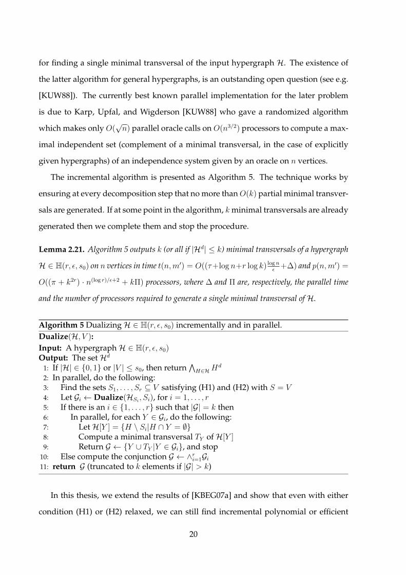
The incremental algorithm is presented as Algorithm 5. The technique works by

ensuring at every decomposition step that no more thanO(k) partial minimal transver-

sals are generated. If at some point in the algorithm, k minimal transversals are already

generated then we complete them and stop the procedure.

Lemma 2.21. Algorithm 5 outputs k (or all if |Hd| ≤ k) minimal transversals of a hypergraph

H ∈ H(r, ε, s0) on n vertices in time t(n,m′) = O((τ+log n+r log k) lognε

+∆) and p(n,m′) =

O((π + k2r) · n(log r)/ε+2 + kΠ) processors, where ∆ and Π are, respectively, the parallel time

and the number of processors required to generate a single minimal transversal ofH.

Algorithm 5 DualizingH ∈ H(r, ε, s0) incrementally and in parallel.Dualize(H, V ):Input: A hypergraphH ∈ H(r, ε, s0)Output: The setHd

1: If |H| ∈ 0, 1 or |V | ≤ s0, then return∧H∈HH

d

2: In parallel, do the following:3: Find the sets S1, . . . , Sr ⊆ V satisfying (H1) and (H2) with S = V4: Let Gi ← Dualize(HSi , Si), for i = 1, . . . , r5: If there is an i ∈ 1, . . . , r such that |G| = k then6: In parallel, for each Y ∈ Gi, do the following:7: LetH[Y ] = H \ Si|H ∩ Y = ∅8: Compute a minimal transversal TY ofH[Y ]9: Return G ← Y ∪ TY |Y ∈ Gi, and stop

10: Else compute the conjunction G ← ∧ri=1Gi11: return G (truncated to k elements if |G| > k)

In this thesis, we extend the results of [KBEG07a] and show that even with either

condition (H1) or (H2) relaxed, we can still find incremental polynomial or efficient

20


parallel algorithms for some classes of hypergraphs as we will see later in Chapter 4

and Chapter 5.

2.5 Related Problems

2.5.1 Dualization of Monotone Boolean Functions

For vectors x = x1, . . . , xn and x′ = x′1, . . . , x′n in 0, 1n, we say x ≤ x′ when each

component of x is less then or equal to the corresponding component of x′ i. e., xi ≤ x′i

for i = 1, . . . , n. A Boolean function f : 0, 1n → 0, 1 is called monotone whenever

for any x, x′ ∈ 0, 1n, x ≤ x′ implies f(x) ≤ f(x′).

A minterm (maxterm) of a monotone Boolean function is a minimal set of variables

which, if all assigned the value 1 (resp., value 0), forces the function to take the value

1 (resp., value 0) regardless of the values assigned to the remaining variables. Any

monotone Boolean function f has unique irredundant (i. e., when no term contains

another) disjunctive normal form (DNF) and conjunctive normal form (CNF)

ϕ =∨F∈F

(∧i∈F

xi

)(2.5)

ψ =∧G∈G

(∨i∈G

xi

), (2.6)

where F ,G ⊆ 21,...,n are Sperner hypergraphs and consist respectively of all minterms

and maxterms of f (cf. [Weg87]). Note that by definition, a maxterm of f is a minimal

set that contains at least one variable from every minterm of f and hence G consists

of all minimal transversals of F i. e., G = Fd. It follows that the following problem is

equivalent to hypergraph dualization.

Input: A monotone Boolean function f given as its irredundant DNF.

Output: The irredundant CNF of f .

Problem DNFTOCNF

The dual of a monotone Boolean function f is denoted by fd and defined as the

function fd(x)def= ¬f(¬x). Note that by definition, (fd)d = f and that a maxterm (resp.

minterm) of f is a minterm (resp. maxterm) of fd. Hence the following problem is also

equivalent to DUALIZATION.

Input: A monotone Boolean function f given as its irredundant DNF.

Output: The irredundant DNF of fd.

Problem BOOLEANDUAL

We define the readability of a monotone Boolean function f to be the minimum in-

teger k such that there exists an ∧-∨-formula equivalent to f in which each variable

appears at most k times. Moreover, we define the size of ∧-∨-formula to be total num-

ber of occurrences of variables in it.

2.5.2 Frequent Sets in Databases

Consider the problem of finding all (inclusion-wise) maximal/minimal collections of

items that are frequently/infrequently bought together by customers in a supermar-

ket. This information for example can be used to optimize the layout of products in

supermarkets and to better predict the trends in demand of certain products. More

precisely, let D ∈ 0, 1m×n be a binary matrix whose rows represent the subsets of

items purchased by different customers in a supermarket. For a given integer t ≥ 0,

a subset of items is said to be t-frequent if at least t rows (transactions) of D contain

it, and otherwise is said to be t-infrequent. Finding frequent item-sets is an essential

problem in finding the so-called association rules in data mining applications [AIS93].

22


See, e.g [AMS+96, BGKM02] for other applications of minimal infrequent and maximal

frequent sets in data mining.

By monotonicity, it is enough to find the border which is defined by the minimal

t-infrequent and maximal t-frequent sets.

Input: A database D ∈ 0, 1m×n and a parameter t.

Output: The family of all maximal t-frequent sets of D.

Problem FREQUENTSETS

Input: A database D ∈ 0, 1m×n and a parameter t.

Output: The family of all minimal t-infrequent sets of D.

Problem INFREQUENTSETS

While it was shown in [BGKM02] that finding maximal frequent sets is an NP-hard

problem, finding the minimal t-infrequent sets turns out to be polynomially equivalent

with the hypergraph transversal problem.

Chapter 3

Fixed Parameter Algorithms

In this chapter we present fixed-parameter algorithms for the hypergraph transversal

problem with the number of edges of the hypergraphs, the minimum integer p such

that the input hypergraph is p-degenerate, and the maximum vertex complementary

degree as our parameters. We conclude with briefly mentioning the FPT results for

DUAL as well as the related problems of generating all maximal independent sets of a

hypergraph and all maximal frequent sets where parameters bound the intersections

or unions of edges.

3.1 Introduction

Briefly, a parameterized problem with parameter k is fixed-parameter tractable if it can

be solved by an algorithm running in time O(f(k) · poly(n)), where f is a function

depending on k only, n is the size of the input, and poly(n) is any polynomial in n. The

class FPT contains all fixed-parameter tractable problems. For more general surveys on

parameterized complexity and fixed-parameter tractability we refer to the monographs

of Downey and Fellows, and Niedermeier [DF99, Nie06].

In this chapter, we show that DUAL(G,H) is fixed parameter-tractable with respect

to the following parameters:

24

CHAPTER 3. FIXED PARAMETER ALGORITHMS 25

• the numbers of edges m = |G| and m′ = |H| (cf. Section 3.2),

• the minimum integer p such that G is p-degenerate (cf. Section 3.3),

• the maximum degrees of vertices in G andH, i. e., d = maxv∈V |G ∈ G : v ∈ G|,

d′ = maxv∈V |H ∈ H : v ∈ H| (cf. Section 3.3),

• the maximum complementary degrees q = maxv∈V |G ∈ G : v /∈ G| and

q′ = maxv∈V |H ∈ H : v /∈ H| (cf. Section 3.4), and

• the maximum c such that |G1 ∪ G2 ∪ · · · ∪ Gk| ≥ n − c, for any G1, . . . , Gk ∈ G

where k is a constant—and the symmetric parameter c′ with respect to H (cf.

Section 3.5).

We shall prove the bounds with respect to the parametersm, d, p, q; the other symmetric

bounds follow by exchanging the roles of G and H. While for parameters c and c′ we

only state the results and point to the literature for further details. Our results for

the parameters m and q improve the respective results from [Hag07]. Moreover, the

bounds we get imply that for parameter size upto logN , we get output polynomial

algorithms, where N = |G|+ |H| is the input and output size of the instance.

In Section 3.5 we also consider the related problem of finding all maximal frequent

sets, which turns out to be fixed parameter-tractable with respect to the maximum size

of the intersection of any k rows of the database D, for a constant k, thus generalizing

the well-known Apriori algorithm, which is fixed-parameter with respect to the size of

the largest transaction.

3.2 Number of Edges as Parameter

Let (G,H) be an instance of DUAL and let m = |G|. We show that the problem is fixed-

parameter tractable with parameter m and improve the running time of [Hag07].

Given a hypergraph G ⊆ 2V and a subset S ⊆ V of vertices, recall from Section 2.2

that S is a sub-transversal of G if there is a minimal transversal T ∈ Gd such that T ⊇ S.

In general, it is an NP-hard to decide if a given subset S is a sub-transversal even if G is

a graph (see [BEGK04]). However, if |S| is bounded by a constant, or if the hypergraph

is read-once [Eit94], then such a check can be done in polynomial time (see [BGH98]).

This observation was used to solve the hypergraph transversal problem in polynomial

time for hypergraphs of bounded edge size or more generally of bounded conformality

in [BEGK04].

The following lemma analyzes the runtime of a brute-force algorithm to decide the

sub-transversal criterion of Proposition 2.8.

Lemma 3.1. Given a hypergraph G ⊆ 2V of size |G| = m and a subset S ⊆ V , of size |S| = s,

checking whether S is a sub-transversal of G can be done in time O(nm(m/s)s).

Proof. For every possible selection G = Gv ∈ Gv(S) | v ∈ S, we can check if G is non-

blocked in O(n|GS|) time. Since the families Gv(S) are disjoint, we have∑

v∈S |Gv(S)| ≤

m, and thus the arithmetic-geometric mean inequality gives for the total number of

selections ∏v∈S

|Gv(S)| ≤(∑

v∈S |Gv(S)|s

)s≤(ms

)s.

Our FPT algorithm uses the backtracking approach of Section 2.4.2 with the sub-

transversal test of Lemma 3.1. Thus, we get the following bound on the running time.

Lemma 3.2. Let G ⊆ 2V be a hypergraph with |G| = m edges on |V | = n vertices. Then

all minimal transversals of G can be found with O(n2m2em/e) delay, where e is the base of the

natural logarithm.

Theorem 3.3. Let G,H ⊆ 2V be two hypergraphs with |G| = m, |H| = m′ and |V | = n. Then

Gd = H can be decided in time O(n2m2e(m/e) ·m′). Thus the problem is FPT with respect to

the parameter m.

Proof. We generate at most m′ members of Gd (if there are more then obviously Gd 6=

H). Assuming that hyperedges are represented by bit vectors (defined by indica-

26


tor functions), we can check whether H is identical to Gd by lexicographically order-

ing the hyperedges of both and simply comparing the two sorted lists. The time to

sort and compare m′ hyperedges each one of size at most log n can be bounded by

O(m′ logm′ log n).

As a side remark we note an interesting implication of Lemma 3.2. Let G be a

hypergraph with |G| ≤ c lnn for a constant c, then Lemma 3.2 finds all its minimal

transversals with polynomial delay O(n2+c/e ln2 n) improving the previous best bound

of O(n6+2c/ log2 e) by Makino [Mak03], where e is the base of the natural logarithm.

3.3 Hypergraph Degeneracy as Parameter

Let G ⊆ 2V be a p-degenerate hypergraph. We show that DUAL(G,H) is fixed-parameter

tractable with parameter p (a result which follows by similar techniques, but with

weaker bounds, from [EGM03]).

As shown in Section 2.1, a p-degenerate hypergraph induced an ordering of ver-

tices v1, . . . , vn such that for 1 ≤ i ≤ n, the degree of a vertex vi in the hypergraph

Gvi,...,vn is at most p. We apply the incremental technique of Section 2.4.3 to dualize

G using the reverse ordering vn, . . . , v1. To this end, let G1,G2, . . . ,Gn be a partition of

hypergraph G defined as Gi = G ∈ G : G 3 vi, G ⊆ vi, . . . , vn. By definition

the size of each set Gi in this partition is bounded by p. This observation yields a sim-

ple FPT algorithm by essentially combining the technique of the previous section with

the incremental method of Section 2.4.3. Recall that the incremental method generates

Gd in time O(|Gd|

(Γ2 + n|G||Gd|

))where Γ2 is the time required to solve smaller sub-

problems which in our case comprises of at most p edges. Using the FPT algorithm of

previous section to solve these smaller instances, we get the following result.

Lemma 3.4. Let G ⊆ 2V be a p-degenerate hypergraph on |V | = n vertices. Then all minimal

transversals of G can be found in time O(n2m′2 ·

(np2ep/e +m

)), where m = |G| and m′ =

|Gd|.

Theorem 3.5. Let G ⊆ 2V be a p-degenerate hypergraph on |V | = n vertices. Then DUAL(G,H)

is fixed parameter tractable with respect to the parameter p.

Since hypergraphs with maximum degree d are also d-degenerate as mentioned

in Section 2.1, the above theorem implies that hypergraph dualization is also fixed

parameter tractable with respect to parameter d.

3.4 Vertex complementary degree as parameter

For a hypergraph G ⊆ 2V and a vertex v ∈ V , consider the number of edges in G

not containing v for some vertex v ∈ V . Let q be maximum such number, i. e., q =

maxv∈V |G ∈ G : v /∈ G|. We show that DUAL(G,H) is fixed-parameter tractable

with parameter q and improve the running time of [Hag07].

We use Proposition 2.16 to decompose the problem into two subproblems (GV \v,HV \v)

and (GV \v,HV \v) not containing a given vertex v ∈ V . Note that the hypergraph GV \vhas at most q edges. This observation leads to a recursive FPT algorithm for vertex

complementary degrees as parameter, by applying Proposition 2.16 at each step, solv-

ing the subproblem (GV \v,HV \v) by applying Theorem 3.3, and recursing on the sub-

problem (GV \v,HV \v). Since at least one vertex is reduced at each step of the algorithm,

there are at most n = |V | recursive steps.

Theorem 3.6. Let G,H ⊆ 2V be two hypergraphs with |G| = m, |H| = m′ and |V | = n. Let

q = maxv∈V |G ∈ G : v /∈ G|. Then Gd = H can be decided in time O(n3q2e(q/e) ·m′).

3.5 Results Based on the Apriori Technique

Gunopulos et al. [GKM+03] showed (Theorem 23, page 156) that generating minimal

transversals of hypergraphs G with edges of size at least n − c can be done in time

O(2cpoly(n,m,m′)), where n = |V |, m = |G| and m′ = |Gd|. This is a fixed-parameter

28


algorithm for c as parameter. Furthermore, this result shows that the minimal transver-

sals can be generated in polynomial time for c ∈ O(log n). The computation is done by

an Apriori (level-wise) algorithm [AS94].

In the following, we briefly mention the results based on apriori technique without

giving the proofs. See [EHR08] and the dissertation of Hagen [Hag08] for details.

Let k and c be two positive integers. We consider hypergraphs G ⊆ 2V satisfying

the following condition:

(C1) Any k distinct maximal independent sets I1, . . . , Ik of G intersect in at most c

vertices, i. e., |I1 ∩ · · · ∩ Ik| ≤ c.

We note that the above property can be verified in polynomial time (see, [EHR08]).

Using the apriori approach, we obtain that we can compute all the maximal in-

dependent sets in time O(min2c(m′)kpoly(n,m), ek/enc+1poly(m,m′)) if any k distinct

maximal independent sets of a hypergraph G intersect in at most c vertices.

Theorem 3.7. If any k distinct maximal independent sets of a hypergraph G intersect in at

most c vertices, then in O(min2c(m′)kpoly(n,m), ek/enc+1poly(m,m′)) time, all maximal

independent sets can be computed, where n = |V |, m = |G| and m′ = |Gdc|.

Equivalently, if the union of any k distinct minimal transversals has size at least

n− c, then all minimal transversals can be computed in the same time bound.

Corollary 3.8. Let G ⊆ 2V be a hypergraph on n = |V | vertices, and k, c be positive integers.

(i) If any k distinct minimal transversals of G have a union of at least n− c vertices, we can

compute all minimal transversals in O(min2c(m′)kpoly(n,m), ek/enc+1poly(m,m′)) time,

where m = G and m′ = |Gd|.

(ii) If any k distinct hyperedges of G have a union of at least n−c vertices, we can compute all

minimal transversals in time O(min2cmkpoly(n,m′), ek/enc+1poly(m,m′)), where m = G

and m′ = |Gd|.

And again using the same idea, we obtain that the maximal frequent sets of an

m× n database can be computed in O(2c(nm′)2k−1+1poly(n,m)) time if any k rows of it

intersect in at most c items, where m′ is the number of such sets.

Theorem 3.9. If any k distinct maximal frequent sets intersect in at most c items, we can

compute all maximal frequent sets in O(2c(nm′)kpoly(n,m)) time, where m′ is the number of

maximal frequent sets.

Corollary 3.10. If any k distinct transactions intersect in at most c items, then all maximal

frequent sets can be computed in time O(2c(nm′)2k−1+1poly(n,m)), where m′ is the number of

maximal frequent sets.

Note that for c ∈ O(log n) and k ∈ O(1) we have incremental polynomial-time

algorithms for all four problems.

30

Chapter 4

r-Exact Hypergraphs

Let H ⊆ 2V be a hypergraph on vertex set V . Recall that H is called r-exact, if any

minimal transversal ofH intersects any hyperedge ofH in at most r vertices. This class

includes several interesting examples from geometry, e.g., circular-arc hypergraphs

(r = 2), hypergraphs defined by sets of axis-parallel lines stabbing a given set of α-fat

objects (r = O(α)), and hypergraphs defined by sets of points contained in translates of

a given cone in the plane (r = 2). For constant r, we give a polynomial-time algorithm

for the duality testing problem of a pair of r-exact hypergraphs. This result implies

that minimal hitting sets for the above geometric hypergraphs can be generated in

incremental polynomial time.

4.1 Introduction

Given an integer r ≥ 1, recall from Chapter 2 that a hypergraphH ⊆ 2V is called r-exact

if

|H ∩ T | ≤ r, for all H ∈ H and T ∈ Hd. (4.1)

As we shall see later, these hypergraphs can be recognized in polynomial time. Clearly,

if H satisfies (4.1) then so do the hypergraphs HS and HS , for any S ⊆ V . Note that

this class of hypergraphs includes the case when max|H| : H ∈ H ≤ r or max|T | :

31

T ∈ Hd ≤ r.

The class of hypergraphs satisfying (4.1) with r = 1, are called exact or read-once

hypergraphs, and are related to a class of monotone Boolean functions also called read-

once functions. We will look at read-once functions in detail in Section 6.2.

For a read-once hypergraph H, the problem of finding Hd is known to be solv-

able with polynomial delay, using a simple backtracking approach [Eit94]. However,

this technique does not seem to generalize for r ≥ 2. Using a more sophisticated

technique, we show in Section 4.3 that the problem can still be solved in incremen-

tal polynomial-time, for any hypergraph satisfying (4.1). The best previously known

result for this class was quasi-polynomial poly(n, |Hd|)|H|O(log |H|) [KBEG07b] (which

gives in fact a global parallel algorithm running in polylogarithmic time and requir-

ing a quasi-polynomial number of processors). In this chapter, we prove the following

theorem.

Theorem 4.1. Let H be an r-exact hypergraph with m edges and n vertices, and k be a

given positive integer. Then for r = O(1), we can find k minimal transversals of H in time

poly(n,m, k).

As consequences of Theorem 4.1, we obtain incremental polynomial-time algo-

rithms for finding:

• all minimal hitting sets, and all minimal set covers, for a circular-arc hyper-

graph (see, e.g., [FS91]). This generalizes known results for interval hypergraphs

[EGM02, BEGK04];

• all minimal hitting sets, and all minimal set covers, for a hypergraph defined by

a set of points and given translates of a certain cone in the plane;

• all minimal subsets of a given set of axis-parallel hyperplanes, hitting a set of

comparable fat objects in Rd, for fixed d (see, e.g., [GIK02, KS06] for the corre-

sponding optimization problems).

32

CHAPTER 4. R-EXACT HYPERGRAPHS 33

We now note that testing a hypergraph H for (4.1) can be done polynomial time, if

r is a constant.

Proposition 4.2. Given a hypergraph H ⊆ 2V and a constant r, whether H is an r-exact

hypergraph can be checked in time O(nr+2mr+3), where n = |V | and m = |H|.

Proof. H satisfies (4.1) if and only if for every edge H ∈ H and every subset X ⊆ H of

size |X| = r+ 1, X is not a sub-transversal toH. For a single subset X of size r+ 1, the

latter condition can be checked in O(nmr+2) time by directly checking the condition of

Proposition 2.8 for a total of O(∑

H∈H( |H|r+1

)nmr+2) time.

The rest of the chapter is organized as follows. In Section 4.2, we give the details of

the geometric applications listed above. Finally, we prove Theorem 4.1 in Section 4.3.

4.2 Applications in geometry

In this section we give some examples of hypergraphs satisfying (4.1) from geometry.

4.2.1 Circular-arc hypergraphs

Let C be a circle in the plane, and V = p0, . . . , pn−1 be a given set of points on C. As-

sume that the points are ordered in clockwise order around C. Let H be a hypergraph

consisting of hyperedges that are defined by consecutive elements of V (that is, arcs

or intervals on the circle, see Figure 4.1). Note that if H is defined by sets of intervals

on the line, then H is both 1-degenerate and 2-Helly (its transpose is 2-conformal), and

hence both problems of finding all minimal hitting sets and of finding all minimal set

covers can be solved in polynomial time [BEGK04, EGM02]. However, if H is defined

by arcs on a circle, then it is not generally k-degenerate, as shown by the following

example: Let H(k, n) be the hypergraph of uniform intervals of length k on a ring of

n = k2 vertices:

H(k, n) = [i : i+ k − 1](mod n)|i = 0, . . . , n− 1.

pi pj pk

Figure 4.1: In a circular-arc hypergraph, every minimal transversal intersects everyinterval at most twice.

Then each vertex has degree k. Furthermore, it is not k-Helly either for any k, as shown

by following hypergraph consisting of k + 1 intervals on a ring of k + 1 vertices:

H(k) = [i : i+ k − 1](mod k + 1)|i = 0, . . . , k.

It is easy to see that any k intervals in H(k) intersect at a common point whereas the

intersection of all intervals is empty.

Nevertheless, we show in the following that ifH is Sperner circular-arc hypergraph,

then every minimal transversal hits every edge inH at most twice.

Proposition 4.3. LetH be a Sperner circular-arc hypergraph. ThenH is 2-exact.

Proof. Let T be a minimal transversal of H, and suppose that |T ∩ H| ≥ 3 for some

H ∈ H. Consider any three points pi, pj, pk ∈ T ∩ H , such that i < j < k (mod n).

Since T is a minimal transversal, there exists H ′ ∈ H such that H ′ ∩ T = pj. But then

H ′ contains neither pi nor pk, and hence H ′ ⊂ H , in contradiction to the fact that H is

Sperner (see Figure 4.1).

Since the transpose of a circular-arc hypergraphH is also circular-arc, we obtain the

following result from Theorem 4.1 and Proposition 4.3.

Corollary 4.4. Let V be a set of points on a circle C and A be a set of circular arcs on C. Then

both problems of finding all minimal sets of points that hit all the arcs in A, and of finding all

minimal sets of arcs that cover all the points can be solved in incremental polynomial time.

Geometrically, the same class can be realized by taking a set of points in convex

position in the plane and defining each edge as a subset of points which lie in some

half-space. However, this does not generalize to higher dimensions.

34


a

a2

a1

p1p3

a1

a

a2

p3 p2

p1

Figure 4.2: The two intersection configurations of the cones C(a1), C(a2) and C(a).

4.2.2 Translates of cones in R2

Let C = x ∈ R2 : aT1 x ≤ 0, aT2 x ≤ 0 be a cone in the plane, where a1, a2 ∈ R2. For a

point a ∈ R2, define C(a) to be the translate of C with apex a, i.e., C(a) = x+ a : x ∈

C. Given a set of apexes A ⊆ R2 and a set of points V ⊆ R2, we define the hypergraph

H(C,A, V ) = V ∩ C(a) : a ∈ A, each hyperedge of which is defined by the subset of

V that lies inside some translate of C (see Figure 4.2).

Proposition 4.5. Let C be a cone in the plane and A, V ⊆ R2. IfH = H(C,A, V ) is Sperner,

thenH is 2-exact.

Proof. Note that for a, a′ ∈ A, C(a) ⊆ C(a′) if and only if a ∈ C(a′). Let T be a minimal

a transversal ofH, and suppose that |T ∩C(a)| ≥ 3 for some a ∈ A. Consider any three

points p1, p2, p3 ∈ T ∩C(a). By minimality of T , there are apexes a1, a2, a3 ∈ A such that

C(ai)∩p1, p2, p3 = pi, for i = 1, 2, 3. We may assume without loss of generality that

C(a1) and C(a2) intersect C(a) as shown in Figure 4.2, right, since otherwise (as shown

in Figure 4.2, left), we have C(a2) ∩ C(a) ⊂ C(a1) ∩ C(a), or vice versa. We observe

that the apex a3 must lie in one of the two shaded regions, for otherwise C(a3) ⊆ C(a),

C(a3) ⊇ C(a1), or C(a3) ⊇ C(a2), in contradiction to the fact that H is Sperner. But if

a3 is contained in the first shaded region then p1 ∈ C(a3), and if it is contained in the

second, then p2 ∈ C(a3), and in both cases we get a contradiction.

Dl

k

v1

v2

vk

Figure 4.3: Left: If we do not require objects to be fat then intersection can be un-bounded. Right: Illustration for Proposition 4.7.

Again, the transpose of H(C,A, V ) can also be realized by translates of a cone, as

implied by a result of Laue [Lau08]. Thus we get the following corollary from Theorem

4.1 and Proposition 4.5.

Corollary 4.6. Let V be a set of points in the plane and C be a set of cones that are translates of

a fixed cone in the plane. Then both problems of finding all minimal sets of points hitting every

cone, and of finding all minimal sets of cones that covers all points can be solved in incremental

polynomial time.

It is not difficult to see that Proposition 4.5 does not generalize to higher dimen-

sions.

4.2.3 Stabbing fat objects in Rd

LetO ⊆ Rd be a d-dimensional object. For α ≥ 1,O is said to be α-fat [Kal97] if the ratio

between the diameter of the smallest ball containing O and the largest ball contained

in O is at most α. For instance, for a ball α = 1, for a hypercube α =√d, and for a line

segment α =∞. The diameter ofO, denoted diam(O), is defined as the diameter of the

smallest enclosing ball.

Let C be a given collection of connected α-fat objects with ρ-comparable diameters,

i.e., diam(O) ≤ ρ · diam(O′), for all O,O′ ∈ C and some constant ρ ≥ 1. Given a

set of axis parallel hyperplanes V , we are interested in finding all minimal subsets of

hyperplanes from V that stab every object in C. Define the hypergraphH(C, V ) = v ∈

V : v stabs O : O ∈ C. We show thatH(C, V ) is O(1)-exact, for fixed d, ρ, and α.

36


Proposition 4.7. Let C be a collection of connected α-fat objects in Rd with ρ-comparable

diameters, and V a set of axis parallel hyperplanes. ThenH(C, V ) is 2αρd-exact.

Proof. Fix an axis ~x, let T be a minimal transversal, and denote by T~x the hyperplanes

in T which are perpendicular to ~x. Assume that some object O ∈ C is hit by k mem-

bers of T~x, say, T~x ∩ v ∈ V : v stabs O = v1, . . . , vk (see Figure 4.3, right). Let

Dl = diam(O) and let D0 be the minimum diameter of enclosed spheres among our

collection of objects C. By minimality of T , there exist objects Oi ∈ C such that T ∩ v ∈

V : v stabs Oi = vi for i = 1, . . . , k. Assume w.l.o.g. that v1, v2, . . . , vk are ordered

along ~x, as in Figure 4.3, right. Observe thatOi,Oi+2 do not intersect for i = 1, . . . , k−2,

since otherwise vi+1 stabs eitherOi, orOi+2, in contradiction to our assumption. There-

fore, we can conclude that Dl ≥ k2D0. Also by the assumption that objects in C are

α-fat and ρ-comparable we have Dl ≤ ραD0. Comparing the two inequalities, we get

k ≤ 2ρα. By applying this argument to every principal axis, we get the result.

Note that fatness is a necessary condition for Proposition 4.7 to hold (see Figure 4.3,

left).

Corollary 4.8. Let C be a collection of α-fat objects in Rd with ρ-comparable diameters, and

V a set of axis parallel hyperplanes. Then for constant α, ρ, d, all minimal sets of hyperplanes

from V stabbing every object in C can be found in incremental polynomial time.

4.3 Dualization of r-exact hypergraphs

To prove Theorem 4.1, we use similar decompositions as the ones used in [KBEG07b].

However, to get a polynomial time algorithm, one uses the fact that duality testing

of two hypergraphs is a symmetric operation with respect to the two hypergraphs.

Combining this with a simple decomposition rule from Proposition 2.16, we can derive

our result.

4.3.1 Decompositions

Let V be a finite set, r ≥ 2 be a positive constant, andH ⊆ 2V be a hypergraph satisfying

(4.1). As it follows from Proposition 2.9, it is enough to solve DUAL(H,G) to prove

Theorem 4.1.

Recall from Section 2.4.5 that a family of sets S1, . . . , Sk ⊆ 2V is a full cover for

H if for every H ∈ H there is an i ∈ [k] such that H ⊆ Si. The main ingredient of our

algorithm is the following decomposition, used (implicitly) in [KBEG07b].

Lemma 4.9. Let H,G ⊆ 2V be hypergraphs satisfying Equation (2.1), and S1, . . . , Sk be a

full cover ofH. Then (H,G) are dual if and only if

(i) for all X ∈ ∧i∈[k] GSi there is a G ∈ G, such that X ⊇ G, and

(ii) (HSi ,GSi) are dual for all i ∈ [k].

Proof. Suppose that (i) does not hold. Then there is an X ∈ ∧i∈[k]GSi such that X 6⊇ G

for all G ∈ G. We note that X is a transversal toH (since the family S1, . . . , Sk is a full

cover and (H,G) satisfy (2.1)). This implies that X satisfies (2.4) with respect to (H,G)

and thus witnessing the fact thatH and G are not dual to each other.

Suppose that (ii) does not hold, i.e., for some i ∈ [k], there is an X ⊆ Si such that X

satisfies (2.4) with respect to the pair (HSi ,GSi). Then X ∪ (V \ Si) satisfies (2.4) with

respect to (H,G).

Suppose now that there is anX that satisfies (2.4) with respect to (H,G). If (ii) holds,

then for every i ∈ [k], there is a Gi ∈ GSi , such that Gi ⊆ X ∩ Si. But then X ⊇ ∪i∈[k]Gi,

and hence there is a Y ∈ ∧i∈[k]GSi such that Y ⊆ X . But (i) implies that Y ⊇ G and

hence X ⊇ G for some G ∈ G, a contradiction.

A symmetric version of Lemma 4.9 can be obtained by exchanging the roles of H

and G and is stated as follows.

Lemma 4.10. Let H,G ⊆ 2V be hypergraphs satisfying Equation (2.1), and S1, . . . , Sk be a

full cover of G. Then (H,G) are dual if and only if

38


(i) for all X ∈ ∧i∈[k]HSi there is a H ∈ H, such that X ⊇ H , and

(ii) (HSi ,GSi) are dual for all i ∈ [k].

Our algorithm also makes use of Proposition 2.16 to partition the problem into two

subproblems.

The above lemmas allow us to reduce a given duality testing problem into smaller

sub-problems. We use (4.1) to define full covers of H and G. For an edge G of G,

consider its partition into r + 1 subsets G1 . . . Gr+1. Since any edge H of H intersects

G in at most r vertices, there would be at least one Gi such that H ∩ Gi is empty. In

other words, if we define Si = V \Gi then for every edge H of H there is an i ∈ [r + 1]

such that H ⊆ Si. However, the covering we get in this way does not necessarily

yield smaller subproblems and may not be balanced and so not much useful for our

divide-and-conquer approach. In the following we present a method to get around

these issues.

For a subset of vertices S, let H(S) denote the set of hyperedges that have at least

one vertex in S, i.e., H(S) = H ∈ H | H ∩ S 6= ∅. Let 0 < ε1 < ε2 < 1/r be

positive constants. Assume that there is an edge G of G such that all of its vertices have

low degrees in H, i.e., degH(v) < ε1|H|, ∀v ∈ G. For an arbitrary ordering v1, . . . , vt

of the vertices of G, let us find the indices i0 = 0 < i1 < · · · < ir+1 = t, such that

|H(vij−1+1, . . . , vij)| ≤ ε2|H| and |H(vij−1+1, . . . , vij+1)| > ε2|H| hold for j = 1, . . . , r.

Note that such indices exist since G is a transversal to H, each vertex in G has degree

less than ε1|H|, and ε1 < ε2 < 1/r. Let us define a partition of G by breaking at these

indices, i.e., Gj = vij−1+1, . . . , vij and let Sj = V \Gj , for j = 1, . . . , r + 1.

We will show that S1, . . . , Sr+1 is a full cover of H with some nice properties.

Notice that for every H ∈ H we have H ⊆ Sj for some j ∈ [r + 1], since |H ∩ G| ≤ r

and so there must exist Gj such that H ∩ Gj = ∅. Also note that |HSj | ≤ ε|H|, for

j = 1, . . . , r + 1, where ε = max rε2, 1− (ε2 − ε1) ∈ (0, 1). Indeed, for j = 1, . . . , r, we

have |HSj | < (1−(ε2−ε1))|H|, since ε2|H| < |H(Gj∪vij+1)| ≤ |H(Gj)|+degH(vij+1) <

|H(Gj)| + ε1|H|. Moreover, |HSr+1| ≤ |H(G1 ∪ . . . ∪ Gr)| ≤∑r

j=1 |H(Gj)| ≤ rε2|H|. In

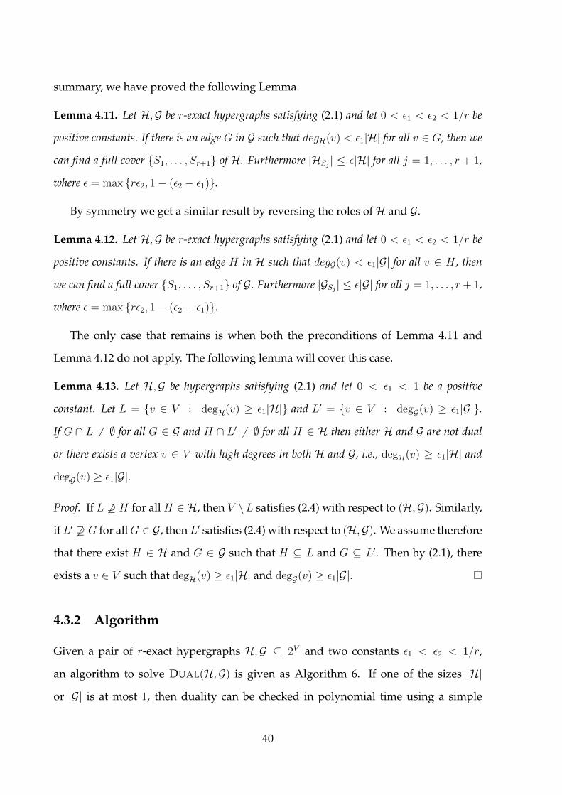
summary, we have proved the following Lemma.

Lemma 4.11. Let H,G be r-exact hypergraphs satisfying (2.1) and let 0 < ε1 < ε2 < 1/r be

positive constants. If there is an edge G in G such that degH(v) < ε1|H| for all v ∈ G, then we

can find a full cover S1, . . . , Sr+1 of H. Furthermore |HSj | ≤ ε|H| for all j = 1, . . . , r + 1,

where ε = max rε2, 1− (ε2 − ε1).

By symmetry we get a similar result by reversing the roles ofH and G.

Lemma 4.12. Let H,G be r-exact hypergraphs satisfying (2.1) and let 0 < ε1 < ε2 < 1/r be

positive constants. If there is an edge H in H such that degG(v) < ε1|G| for all v ∈ H , then

we can find a full cover S1, . . . , Sr+1 of G. Furthermore |GSj | ≤ ε|G| for all j = 1, . . . , r + 1,

where ε = max rε2, 1− (ε2 − ε1).

The only case that remains is when both the preconditions of Lemma 4.11 and

Lemma 4.12 do not apply. The following lemma will cover this case.

Lemma 4.13. Let H,G be hypergraphs satisfying (2.1) and let 0 < ε1 < 1 be a positive

constant. Let L = v ∈ V : degH(v) ≥ ε1|H| and L′ = v ∈ V : degG(v) ≥ ε1|G|.

If G ∩ L 6= ∅ for all G ∈ G and H ∩ L′ 6= ∅ for all H ∈ H then either H and G are not dual

or there exists a vertex v ∈ V with high degrees in both H and G, i.e., degH(v) ≥ ε1|H| and

degG(v) ≥ ε1|G|.

Proof. If L 6⊇ H for all H ∈ H, then V \L satisfies (2.4) with respect to (H,G). Similarly,

if L′ 6⊇ G for allG ∈ G, then L′ satisfies (2.4) with respect to (H,G). We assume therefore

that there exist H ∈ H and G ∈ G such that H ⊆ L and G ⊆ L′. Then by (2.1), there

exists a v ∈ V such that degH(v) ≥ ε1|H| and degG(v) ≥ ε1|G|.

4.3.2 Algorithm

Given a pair of r-exact hypergraphs H,G ⊆ 2V and two constants ε1 < ε2 < 1/r,

an algorithm to solve DUAL(H,G) is given as Algorithm 6. If one of the sizes |H|

or |G| is at most 1, then duality can be checked in polynomial time using a simple

40


procedure Dual-Simple() from Section 2.4.1.1. Otherwise, the algorithm first tries to

apply the decompositions of Lemma 4.11 and Lemma 4.12. If both cases do not apply,

then Lemma 4.13 guarantees the existence of a high degree vertex in both hypergraphs,

which we use to partition our problem by applying Proposition 2.16.

The following lemma gives a bound on the number of iterations t(v) in terms of

v = |H||G|, n = |V | and ε = max 1− ε1, rε2, 1− (ε2 − ε1) ∈ (0, 1), where ε1 = 12r+1

and

ε2 = 22r+1

give us the best ε obeying the given constraints.

Lemma 4.14. t(v) = Θ (nvr+1) .

Proof. Consider a particular iteration of the procedure. If the conditions in Step 4 or 13

becomes true, we get the recurrence

t(v) ≤ nvr+1 + (r + 1)t(εv), (4.2)

while in Step 15, we get the recurrence

t(v) ≤ nv + 2t(εv). (4.3)

Clearly, the recurrence (4.2) dominates the recurrence (4.3) when r ≥ 1. Applying

Akra-Bazi theorem [AB98] on the recurrence (4.2) yields the stated claim.

4.4 Conclusions

In this chapter, we have shown how to dualize r-exact hypergraphs in output poly-

nomial time when r is a constant. We also have given some examples of geometric

hypergraphs which are r-exact for a constant r. In the next chapter, we will show how

to dualize a broader class of geometric hypergraphs in output polynomial time.

Algorithm 6 Dualizing r-exact hypergraphsProcedure Duality(H,G, V, ε1, ε2):Input: r-exact hypergraphsH,G ⊆ 2V , and positive constants 0 < ε1 < ε2 < 1/r.Output: Returns true if (H,G) are dual, returns a witness of non-duality otherwise.

1: if min|H|, |G| ≤ 1 then2: return Dual-Simple(H,G).3: Let L = v ∈ V : degH(v) ≥ ε1|H| and L′ = v ∈ V : degG(v) ≥ ε1|G|.4: if (∃G ∈ G, G ⊆ V \ L) then5: Let S1, . . . , Sr+1 be a full cover ofH (Lemma 4.11)6: Call Duality(HSi ,GSi , ε1, ε2) for all i ∈ [r + 1]7: if any call in Step 6 fails then8: return the corresponding witness of non-duality9: for all X ∈ ∧i∈[r+1] GSi do

10: if there is no G ∈ G such that X ⊇ G then11: return X as a witness of non-duality12: return true13: else if (∃H ∈ H, H ⊆ V \ L′) then14: Repeat Steps 5-12 with the roles ofH and G reversed15: else if (∃v ∈ V such that degH(v) ≥ ε1|H| and degG(v) ≥ ε1|G|) then16: Call Duality(HV \v,GV \v, ε1, ε2); Call Duality(HV \v,GV \v, ε1, ε2)17: if any call in Step 16 fails then18: return a witness of non-duality19: return true20: else21: return a witness of non-duality (Lemma 4.13)

42

Chapter 5

Geometric Hypergraphs

In this chapter, we present two approaches to dualize geometric hypergraphs, i. e., hy-

pergraphs arising from geometric objects in Rd for a fixed d. The two general frame-

works which are presented in Section 5.2 and Section 5.3 yield incremental polynomial

algorithms for several types of geometric hypergraphs. While the first approach uses

elementary techniques, the second one relies on simplicial partitions and cuttings, and

yields global parallel dualization algorithms for a larger class of hypergraphs. In Sec-

tion 5.4, we present a polynomial delay algorithm for hypergraphs defined by sets of

points and half-planes in R2.

5.1 Introduction

Let P ,Q be two families of geometric objects in Rd for a fixed d. Associating a vertex

with each member of P , we define a hypergraph (P ,Q) induced by these two families

as (P ,Q) = P ∈ P|P ∩ Q 6= ∅ |Q ∈ Q. In this chapter, we will often refer to

hypergraphs as range spaces in accordance with the terminology in the Computational

Geometry literature. Accordingly, we will refer to the vertex set as the ground set and

the hyperedges as ranges. There are two natural range spaces defined by P and Q

depending on whether we let P or Q form the ground set. We denote by (P ,Q) the

range space in which P is the ground set and each Q ∈ Q defines the range P ∈

43

P|P ∩ Q 6= ∅ as defined above. Similarly, we denote by (Q,P) the range space in

which the ground set is Q and each P ∈ P defines the range Q ∈ Q|Q ∩ P 6= ∅. Note

that (Q,P) = (P ,Q)t.

When P is a set of points and Q be a set of geometric objects then (P ,Q)d is the set

of all minimal hitting sets of Q, while (Q,P)d is the set of all minimal set covers of P .

In this chapter, we introduce general frameworks to solve the hypergraph transver-

sal problem for geometric hypergraphs as introduced above. The first approach, pre-

sented in Section 5.2, uses only elementary techniques, and gives polynomial-time al-

gorithms for the problems of hitting axis-parallel hyper-rectangles by points and stab-

bing connected objects by axis-parallel hyperplanes, both in Rd for a fixed d. In Section

5.3, we present another technique based on simplicial partitions and cuttings, to effi-

ciently enumerate all minimal hitting-sets as well as minimal covers of hypergraphs

defined by the intersection of sets of points with half-spaces (and hence balls) or more

generally, polytopes with a constant number of facets all in fixed dimension Rd. Finally,

in Section 5.4 we give a polynomial delay algorithm for the special case of hypergraphs

induced by half-planes and points in R2.

The enumeration of minimal geometric hitting sets, as the ones described above,

arises in various areas such as computational geometry, machine learning, and data

mining [EMG08]. Moreover, our efficient enumeration algorithms might be useful in

developing exact algorithms, fixed-parameter tractable algorithms, and polynomial-

time approximation schemes for the corresponding optimization problems (see, e.g.,

[HNW08]).

5.2 First Approach: Using Elementary Techniques

This section presents a general framework for the problem of finding all minimal hit-

ting sets of a family of objects in Rd by another. It can be regarded as a generalization

of the algorithms given in [EGM03, LLK80], i. e., the incremental approach of Section

44

CHAPTER 5. GEOMETRIC HYPERGRAPHS 45

2.4.3. We apply it to the following problems:

• Hitting hyper-rectangles by points: Given a finite set of points P ⊆ Rd and

a finite collection F of axis-parallel hyper-rectangles (also called orthotopes or

boxes) in Rd, find all minimal sets of points from P that hit every hyper-rectangle

in Q;

• Hitting (Stabbing) connected objects by axis-parallel hyperplanes: Given a fi-

nite set of axis-parallel hyperplanes P ⊆ Rd and a finite collectionQ of connected

objects in Rd, find all minimal sets of hyperplanes from P that stab every object

in Q.

We show that the above two problems can be solved in incremental polynomial time,

if the dimension d of the underlying space is fixed.

In the next section, we give a general framework for finding all minimal hitting

sets for a given hypergraph. In Sections 5.2.2 and 5.2.3 we apply this framework to

the problem of hitting hyper-rectangles by points and stabbing connected objects by

axis-parallel hyperplanes respectively.

5.2.1 A Framework for Computing Transversal Hypergraphs

Let H be a hypergraph on a set V = 1, . . . , n. Recall the incremental approach of

Section 2.4.3 that divides the problem of computing Hd into several sub-problems of

the same type. The key fact behind the framework presented in this section is that for

some geometric hypergraphs if we recurse on these sub-problems then we make some

progress so that the process eventually terminates.

Given an ordering σ of vertices and for i = 1, . . . , n, let Hi be the sub-hypergraphs

of H defined as Hi = H ∈ H : σ(i) ∈ H and H ⊆ σ(1), . . . , σ(i) and let ∆i[X] =

H ∈ Hi : H ∩X = ∅. A framework based on incremental approach of Section 2.4.3

is presented as Algorithm 7. The algorithm proceeds inductively, for i = 1, . . . , n, by

extending each minimal transversal X in (H1∪ . . .∪Hi−1)d to a set in (H1∪ . . .∪Hi)d by

recursively finding (∆i[X])d, each set of which is combined withX to obtain a minimal

transversal of (H1 ∪ . . . ∪Hi).

Algorithm 7 A framework to compute minimal transversals of geometric hypergraphProcedure Dualize1(H,Σ, j):Input: A hypergraph H over V = 1, . . . , n, an index j (≤ k) and a sequence Σ =

(σ1, . . . , σk) of permutations of vertices in V .Output: The hypergraphHd.

1: H0 ← ∅, X0 ← ∅, Xi ← ∅ ∀i = 1, . . . , n2: for i = 1, . . . , n do3: LetHi ← H ∈ H : σj(i) ∈ H and H ⊆ σj(1), . . . , σj(i)4: for all X ∈ Xi−1 do5: Let ∆i[X] = H ∈ Hi : H ∩X = ∅6: if j = k or |∆i[X]| ≤ 1 then7: A ←Dualize-Simple(∆i[X])8: else9: A ←Dualize1(∆i[X],Σ, j + 1)

10: Xi ← min (Xi⋃ X ∪ Y : Y ∈ A)

11: return Xn

The algorithm uses a sequence of permutations Σ = σ1 . . . σk as a part of the input.

When called initially as Dualize1(H,Σ, 1), it dualizesH by using the above mentioned

approach where σj is used for partitioning in the j-th level of the recursion. After k

levels of recursion, procedure Dualize-Simple() is used directly to solve the problem.

As we will see in the later sections, for several classes of geometric hypergraphs, the

subproblem after k levels can be solved easily, where k depends only on the dimension

of the geometric space under consideration.

As an illustration, consider the problem of dualizing an interval hypergraph: Let

V = p1, p2, . . . , pn be a set of points on the line ordered from left to right, and let

H ⊆ 2V be a Sperner hypergraph, in which each edge H ∈ H consists of consecutive

points from V . Denote by σ the left-to-right ordering of the vertices, and consider

the execution of the Algorithm 7 when called as Dualize1(H,Σ, 1) with Σ = σ. The

algorithm incrementally dualizes the hypergraphs Hi = H ∈ H : pi ∈ H and H ⊆

p1, . . . , pi for i = 1 . . . n. Note that the subproblem ∆i = Hi contains at most one

edge because of our assumption thatH is Sperner and thus can be solved trivially.

46


vi vi+1

vi′

vi′−1

vi vi+1

vi′

vi′−1

Figure 5.1: An example of points and rectangles in R2. Left: The set ∆i consists of all rectanglesthat contain vi and other points only from the subset v1, . . . , vi. Right: The subproblem in therecursive call considers all rectangles which contain both vi and vi′ and no points from the strictleft of vi′ nor from the strict right of vi

The correctness of the procedure follows from Proposition 2.10 and the correctness

of the procedure Dualize-Simple. From Lemma 2.15 and the fact that Algorithm 7

recurses until depth at most k, we get the following bound on the worst-case running

time.

Theorem 5.1. Let H ⊆ 2V be a hypergraph over vertex set V and Σ = (σ1, . . . , σk) be a se-

quence of permutation functions of vertices ofH. Then procedure Dualize1(H,Σ, 1) computes

Hd in O((nm′)k(mm′ + T )) time, where n = |V |, m = |H|, m′ = |Hd| and T is time required

by Dualize-Simple() in each k-th level recursion of the procedure.

5.2.2 Points and Hyper-rectangles in Rd

Let P be a set of points and Q be a collection of axis-parallel hyper-rectangles in Rd.

In this section, we consider the problem of enumerating all minimal hitting sets of the

hypergraph (P ,Q). LetH ⊆ 2P be the hypergraph (P ,Q).

To illustrate the idea, let us first consider the problem in R2. The algorithm is based

on the framework presented as Algorithm 7. We order the points in P from left to right

and if their x-coordinates are equal, we sort them from bottom to top. Let v1, v2, . . . , vn be

the corresponding ordering of the vertices of the hypergraph H ⊆ 2P , defined above.

Note that because of our ordering of the vertices, no rectangle in the hypergraph Hi

contains any point strictly to the right of vi and by definition, every rectangle in ∆i ⊆

Hi contains vi.

Consider the subproblem of dualizing ∆i[X] for each i ∈ [n] and X ∈ (Hi−1)d and

let the primed variables denote the corresponding variables in the recursive call of the

algorithm. We order the vertices of H′ = ∆i[X] in the reverse order i. e., from right to

left, breaking ties by sorting them from top to bottom.

Consider now a further recursive call of the procedure on a hypergraph H′′ =

∆′i′ [X′], where i′ ∈ 1, . . . , |V (H′)| and X ′ ∈ (H′i′−1)d. The crucial observation is that

each rectangle corresponding to an edge in the hypergraph ∆′i′ [X′] contains both the

points vi and vi′ , and because of our ordering, no rectangle in the subproblem con-

tains a point from the left of vi′ nor from the right of vi (see Figure 5.1). Hence, as

can be easily seen, only the y-coordinates matter when deciding whether a given point

v ∈ vi′ . . . vi intersects a rectangle from ∆′i′ [X′]. So we can project the subproblem

∆′i′ [X′] on the y-axis and reduce it to a problem of dualizing an interval hypergraph,

which can be solved in polynomial time, as seen in Section 5.2.1.

The above algorithm can be extended to higher dimensions in an obvious manner.

In dimension d, we use the orderings Σ = (σ1, . . . , σ2d−2), where σi is the lexicographical

ordering of the points using their last d − b i−12c coordinates. Moreover, we define the

ordering σi to be increasing when i is odd and decreasing otherwise. To generate all mini-

mal transversals ofH, we call Dualize1(H,Σ, 1), and use the dualization procedure for

interval hypergraphs in place of Dualize-Simple(). After the second recursive call the

subproblems we obtain contain all hyper-rectangles that intersect two given points,

say vi′ and vi with vi′ being lexicographically smaller than vi, and have the property

that they contain no point that is lexicographically smaller then vi′ or lexicographically

greater than vi. Hence after two levels of recursion, the first coordinate of the points

can be ignored and thus the problem reduces to d− 1-dimensional subproblems.

5.2.3 Stabbing Connected Objects in Rd

Given a collection of connected objectsQ and a set of axis-parallel hyperplanes P , both

in Rd, we are interested in the problem of finding all minimal sets of hyperplanes from

48


v4

v3

v2

v5

v6 v7 v9 v10v8

v1

vi−1 vi+1vi

Figure 5.2: Left: An example of lines and objects in R2 and a valid ordering of lines. Right: Theset ∆i[X] consists of new objects that intersect vi and only lines from the subset v1, . . . , vi−1.

P such that every object in Q is stabbed by at least one of the hyperplanes in the set.

Let H = (P ,Q) be the corresponding hypergraph with vertex set P and each object

Q ∈ Q defining an edge consisting of all hyperplanes from P which intersect Q.

We consider the simple case first, that is, when all hyperplanes in P are parallel to

each other. This turns out to be equivalent to the interval hypergraph case since we can

project the objects inQ on any line L that is perpendicular to the hyperplanes in P . The

projection maps hyperplanes in P into points on L, and because of the connectedness,

the objects in Q are mapped to intervals on L.

More generally, for d > 1, assume there is at least one hyperplane perpendicular

to every principal axis. The assumption can be made without loss of generality, since

if there is no hyperplane along a particular principal axis, say z, then we can orthogo-

nally project all other hyperplanes and objects on the hyperplane z = 0 and reduce the

dimension of the problem by one.

The dual of H can be found incrementally by following Algorithm 7. Fixing the

order of principal axes, we order the hyperplanes sequentially: starting with hyper-

planes perpendicular to the first principal axis, sorted in increasing order, we continue

with the hyperplanes perpendicular to the second principal axis and so on. For an

example in R2, the set of lines x = 1, y = −1, x = 0, y = 1 would be ordered as

x = 0, x = 1, y = −1, y = 1 assuming that x-axis comes before y-axis in our fixed or-

dering of principal axes. Let σ be an ordering of hyperedges of H as defined above

and let jH0 < jH1 < . . . < jHd be indices with jH0 = 0 and jHd = n, such that the cor-

responding hyperplanes in the group σ(jHr−1 + 1), . . . , σ(jHr ) are parallel to each other

and perpendicular to r-th principal axis for r ∈ [d].

Consider the subproblem of dualizing Hi for i = 1, . . . , n as defined in the al-

gorithm, where Hi contains only those edges which form subsets of vertices from

vσ(1), . . . , vσ(i). As discussed above, the problem reduces to dualizing an interval hy-

pergraph when 1 ≤ i ≤ jH1 . Now consider the case when jHr−1 < i ≤ jHr for r ∈ [d].

Consider the subproblem of dualizing H′ = ∆i[X] for X ∈ (Hi−1)d, and let the primed

variables denote the corresponding variables in the recursive call of the algorithm.

Note that the subproblem for ∆i[X] contains all objects that do not intersect any hy-

perplane “above” vσ(i). Let σ′ be an ordering of vertices of H′ defined similarly as σ

for the hyperplanes perpendicular to first r − 1 principal axes except the r-th group

of hyperplanes which are sorted in decreasing order. As before, let jH′0 < . . . < jH′

r be

indices with jH′0 = 0 and jH′r = n′, where n′ = |V (H′)| and the hyperplanes in the group

σ′(jH′

r′−1 + 1), . . . , σ′(jH′

r′ ) are parallel to each other and perpendicular to r′-th principal

axis for r′ ∈ [r].

In the recursive call, we use σ′ as our ordering and dualize H′ incrementally by

considering H′i′ for 1 < i′ ≤ i. Note that for i′ ≤ jH′

r−1, V (H′i′) ⊆ V (Hi−1) and hence the

subproblemH′i′ is already taken care of when (Hi−1)d is computed. Alternatively, when

jH′

r−1 < i′ ≤ i then similar to the case in Section 5.2.2, the subproblems ∆′i′ we get contain

all objects that intersect both vi and vi′ with the property that no hyperplane above vi

or below vi′ stabs any of them. Note that both vi and vi′ as well as all hyperplanes

between them are trivially hitting sets for the subproblems for hypergraphs of the form

∆′i′ [·]. The other hitting sets can be found recursively by observing that they do not

involve any of the hyperplanes parallel to vi and vi′ . Thus we are able to reduce the

dimension of the problem by 1 after two levels of recursion.

In summary, to generate H, we call Dualize1(H,Σ, 1) with Σ = (σ1, σ2, . . . , σ2d−1)

and a trivial dualization procedure for Dualize-Simple(). For odd r, 1 ≤ r < 2d, the

50


ordering σr sorts each group of parallel hyperplanes in increasing order (of the points

of intersection with the common orthogonal line), whereas for even r, 1 < r < 2d,

σr is defined by sorting each group of parallel hyperplanes in increasing order except

the last group, which is sorted in decreasing order (of the points of intersection with

the common orthogonal line). As we noted above, at every r-th level of recursion for

even r, the dual hypergraphs Hdi such that vσ(i) does not belong to the last group of

hyperplanes, can be easily computed from the corresponding dual hypergraph in the

recursion level r − 1. This observation can be used to avoid redundant computations

by solving those subproblems directly instead of following the Algorithm 7.

5.3 Second Approach: Using Cuttings and Simplicial Par-

titions

In this section, we show that, when the hypergraph (P ,Q) admits a balanced subdivision,

then a recursive decomposition can be used to obtain efficiently all minimal hitting

sets of the hypergraph. We apply this decomposition framework to get incremental

polynomial-time algorithms for finding minimal hitting sets and minimal set covers

for a number of hypergraphs induced by a set of points and a set of geometric objects.

The set of geometric objects includes half-spaces, hyper-rectangles and balls, in fixed

dimension.

5.3.1 Introduction

As compared with previous section, the framework of this section is simpler and it

works for both the hitting set and set covering versions, and extends to more gen-

eral objects, such as balls, half-spaces, and polytopes with fixed number of facets. In

fact, as we will see, all that is needed is that the hypergraph admits a certain balanced

subdivision which can be shown to exist in several geometric instances. One more im-

portant property of the algorithms we obtain, is that they admit a global parallel im-

plementation, in the sense that all minimal hitting sets can be generated in polyloga-

rithmic time using a polynomial number of processors. Among all polynomially solv-

able classes of hypergraphs, only very few are known to exhibit this nice property, see

[KBEG07a, KBGE07].

Our algorithm is based on recursive decompositions of the space, and builds on

the full cover decompositions, introduced in Section 2.4.5. In the following, we show

that a modified version of a full cover can be combined with simplicial partitions and

cuttings, to define a large class of hypergraphs for which full cover decompositions are

effective.

The rest of Section 5.3 is organized as follows: In Section 5.3.2, we describe the type

of decomposition used in the algorithm and show how it can be achieved for vari-

ous geometrically induced range spaces using simplicial partitions and cuttings. We

present the algorithm and analyze it in Section 5.3.3. We conclude with an applica-

tion of generating minimal hitting sets of hypergraphs to a problem in mining spatial

databases.

5.3.2 Balanced Subdivisions

Given any range space (P ,Q), we say that a subset P ′ ⊆ P is stabbed by a range Q ∈ Q

if there exist x, y ∈ P ′ s.t. x ∈ Q and y /∈ Q. A balanced subdivision for a range space

(P ,Q) is a collection of a constant number of subsets P1,P2, . . . ,Pλ of P such that

1. For each i ∈ 1, . . . , λ, |Pi| ≥ ε|P| for some constant 0 < ε ≤ 1.

2. For each range Q ∈ Q, there are two disjoint subsets Pi and Pj in the collection

which are not stabbed by Q.

Remark 5.2. In the above definition, the fact that a subset P ′ ⊂ P is not stabbed by Q ∈ Q

implies that P ′ is also not stabbed by P \ Q. Consequently, we conclude that a balanced sub-

division for any range space (P ,Q) is also a balanced subdivision for the range space (P ,Qc),

52


where Qc denotes the compliments of ranges in Q, i. e., Qc = Rd \Q | Q ∈ Q.

In the next section, we show that if we can compute a balanced subdivision for a

range space then we can enumerate its minimal hitting sets in global parallel time.

In this section, we show that several geometrically induced range spaces admit

balanced subdivisions which can be computed efficiently (in parallel). Specifically, we

show that for any point set P ⊂ Rd, a balanced subdivision exists and can be computed

efficiently for both (P,H) and (H, P ) if H is a family of objects of the following kind:

(i) Half-Spaces in Rd (ii) Polytopes with a constant number of facets in Rd and (iii) Balls

in Rd.

We will use the following results:

Theorem 5.3 (Fine Simplicial Partitions [Mat92]). Given any set P of n points in Rd and

any parameter 1 ≤ r ≤ n, there exists a partition Π = P1, P2, . . . , Pt of t ≤ r disjoint subsets

of P and a set ∆ = ∆1, . . . ,∆t of simplices with the following properties: (i) Pi ⊆ ∆i (ii)⋃i Pi = P , (iii) n/r ≤ |Pi| ≤ 2n/r for all i ∈ 1, . . . , t and (iv) no half-space in Rd

intersects more than Cdr1−1/d of the simplices in ∆, where Cd is a constant for any fixed d. The

last property also implies that no half-space in Rd stabs more than Cdr1−1/d of the sets in Π.

Further, for any δ > 0, such a Π can be computed in time O(n1+δ). When r is bounded by a

constant, Π can be computed in O(n) time.

Theorem 5.4 (Cuttings [Cha93]). Given any set of n half-spaces in Rd and any parameter

1 ≤ r ≤ n, there exists a partition of Rd into r simplices such that none of the simplices

is stabbed by more than C ′dn/r1/d of the given half-spaces. Further, for any δ > 0, such a

partition can be computed deterministically in time O(nr1−1/d).

Parallel Implementation: Even though we only mention sequential running times

above, such fine simplicial partitions and cuttings can be computed in polylog(n) time

using poly(n) processors. For example, in the case of cuttings in any fixed dimension

d, while the simplices are allowed to be arbitrary, it can be argued that they can always

be chosen so that they are among a polynomial number of canonical simplices. In fact,

it is not hard to argue that we can restrict to simplices whose corners are defined by the

intersection of d of the hyperplanes defining the given set of halfspaces and indeed the

construction in [Cha93] does restrict to such simplices. The number of such simplices

is at most O(nd(d+1)). Once we have a polynomial bound on the number of canoni-

cal simplices, we can check all possible sets of t canonical simplices in parallel using

a polynomial number of processors and find a simplicial partition in polylogarithmic

time. A similar argument holds for simplicial partitions.

Half-Spaces. Let us first consider the case when H is a set of half-spaces in Rd. Given

any set P with n points in Rd, we can set r to be a large enough constant so that

Cdr1−1/d ≤ r − 2. Then, clearly, the collection Π given by Theorem 5.3 also gives us

a balanced subdivision of (P,H) with ε = 1/r and k ≤ r. To get a balanced subdivision

of (H, P ), we apply Theorem 5.4 to the half-spaces inH. Assuming that |H| = n, we set

r to be a large enough constant so that C ′dn/r1/d ≤ n/2. Theorem 5.4 gives a partition

of Rd into r regions R1, . . . , Rr each of which is stabbed by at most n/2 half-spaces in

H. Consequently, for each region Ri, we either have at least n/4 half-spaces of H each

of which contains Ri or we have at least n/4 half-spaces of H none of which intersects

Ri. Let Hi be a set of those half-spaces. Then |Hi| ≥ n/4. We arbitrarily partition each

Hi into two disjoint sets H1i and H2

i each of size at least n/8. These sets H1i and H2

i for

i ∈ 1, . . . , r give us a balanced subdivision of (H, P ) with k = 2r and ε = 1/8 since

each point p ∈ P lies in some region Rj and hence does not stab the disjoint sets H1j

andH2j .

Remark 5.5. In the case of half-spaces, one may also reduce the problem of finding minimal set

covers to that of finding minimal hitting sets by using geometric duality, which maps points

in Rd to hyperplanes and vice versa (see e.g. [dBvKOS97], Chapter 8). However this method

does not work for polytopes.

Polytopes. Suppose now thatH is a set of polytopes in Rd, each with at most f facets.

In this case the collection Π given by Theorem 5.3 with r being a large enough constant

54


so that f ·Cdr1−1/d ≤ r−2 gives us the required balanced subdivision for (P,H). This is

because each facet of a polytope can stab at most Cdr1−1/d members of Π and therefore

a polytope with at most f facets can stab at most f ·Cdr1−1/d ≤ r− 2 members of Π. To

get a balanced subdivision for (H, P ), we consider for each H ∈ H, the set of at most

f half-spaces whose intersection forms H . Let H′ be the set of all these half-spaces.

Assuming that |H| = n, we have that |H′| ≤ fn. We then invoke Theorem 5.4 for

the half-spaces in H′ with r being a large enough constant so that C ′d(nf)/r1/d ≤ n/2.

The regions in the resulting partition are stabbed by at most n/2 half-spaces in H′ and

hence at most n/2 polytopes in H. We can then construct the balanced subdivision for

(H, P ) consisting of setsH1i andH2

i , i ∈ 1, . . . , r, as in the last paragraph.

Balls. Finally assume thatH is a set of balls in Rd. There is a standard lifting (Veronese

map) which maps each point in Rd to a point in Rd+1 and each ball in Rd to a half-

space in Rd+1 so that the incidence relations among them are preserved. Since balanced

subdivisions exist for half-spaces in Rd+1, we can conclude that balanced subdivisions

exist for balls in Rd as well (for both (P,H) and (H, P )).

Since we invoke Theorems 5.3 and 5.4 with r being a constant, the collection in

Theorem 5.3 and the partition in Theorem 5.4 can be computed in time O(n). It follows

that balanced subdivisions for the above range spaces can be computed in O(n + m)

time where n is the size of the ground set and m is the number of ranges.

5.3.3 The Enumeration Algorithm

Given a range space (P ,Q), a divide-and-conquer algorithm to enumerate all minimal

hitting sets ofQ is presented as Algorithm 8. If |P| is at most some fixed constant µ, we

use the procedure Dualize-Simple from Section 2.4.1.1 for the enumeration of minimal

hitting sets in these trivial cases.

When |P| > µ, we assume the existence of a balanced subdivision Π = (P1, . . . ,Pλ),

where λ is a constant and for each i ∈ 1, . . . , λ, |Pi| ≤ ε|P| where 0 < ε < 1 is

another constant. We classify the minimal hitting sets of Q into two types. Type 1

Algorithm 8 Procedure Dualize(P ,Q):Input: A finite range space (P ,Q)Output: The set of all minimal hitting sets of Q

1: if |P| ≤ µ then2: return Dualize-Simple(P ,Q)3: Type1-Set:=∅4: Compute a balanced subdivision P1, . . . ,Pλ of (P ,Q)5: for i = 1, . . . , λ do6: Type1-Set := Type1-Set ∪ Dualize(P \ Pi,QP\Pi)7: Type1-Set := Remove-Duplicates(Type1-Set)8: Type2-Set := ∅9: for i = 1, . . . , λ do

10: Xi := Enumerate(P \ Pi,QP\Pi)11: for each (M1, . . . ,Mλ) ∈ X1 × . . .×Xλ do12: M :=

⋃iMi

13: if M is a type 2 minimal hitting set of Q then14: Type2-Set := Type2-Set ∪ M15: Type2-Set := Remove-Duplicates(Type2-Set)16: return Type1-Set ∪ Type2-Set

minimal hitting sets are those that have an empty intersection with one of the Pis.

The remaining minimal hitting sets which contain elements from each Pi are of type 2.

Note that by Corollary 2.13, (Qd)P\Pi = (QP\Pi)d, and so type 1 hitting sets are easily

enumerated recursively. This is done in line 6 of Algorithm 8. Enumerating Type 2

minimal hitting sets requires more work.

Let us first recall that any minimal hitting set M of Q and for any v ∈ M , there is

always some range Q ∈ Q which requires v, i.e., Q ∩M = v. We call such a range

a certificate range for v in M . Clearly, M is also a minimal hitting set for the set of

certificate ranges of its elements.

Let M be any type 2 minimal hitting set and let Q ∈ Q be any range that has a

nonempty intersection with each of the Pis. Since Π is a balanced subdivision, there

are at least two sets Pj and Pk which are not stabbed by Q. Since Q has a nonempty

intersection with both of them, it must contain both the sets as subsets. Now, since M

contains an element from each Pi, Q contains at least two elements of M implying that

Q cannot be a certificate range for any element of M . This means that for the purpose

56


of enumerating type 2 minimal hitting sets, we can discard all ranges which have a

non-empty intersection with each of the Pis. Let Qi = QP\Pi and let Q =⋃iQi.

Let M be any type 2 minimal hitting set ofQ. Since Q contains all certificate ranges

of M , M is also a minimal hitting set for Q. Also, since the ranges in Qi do not contain

any element of Pi, M \ Pi is a hitting set (not necessarily minimal) forQi and therefore

contains some Mi ⊆M \ Pi which is a minimal hitting set for Qi.

Note that each element ofM appears in at least one of theMis, since each v ∈M has

a certificate range Q which belongs to some Qi implying that v ∈ Mi. In other words,

M =⋃iMi. This suggests the following algorithm for enumerating the minimal hitting

sets of type 2. For each i ∈ 1, . . . , λ, recursively compute the set Xi of all minimal

hitting sets of (V \ Vi,Qi). Then, try all possible ways of picking one minimal hitting

set Mi ∈ Xi from each Xi and output M =⋃iMi if it is a type 2 minimal hitting set

for Q. This way we surely enumerate all type 2 minimal hitting sets. Now, we need

to bound the number of combinations we try. We get this from Proposition 2.12 which

implies that |Xi| ≤ |Qd|.

Let T be the number of minimal hitting sets of Q. It follows that the number of

combinations of Mi’s we need to try is at most T λ. After we find all type 1 minimal

hitting sets we run a procedure called Remove-Duplicates to remove any duplicates

we may have generated. Similarly, after we find all type 2 minimal hitting sets, we run

Remove-Duplicates to remove any duplicates. This ensures that in the end we do not

output any duplicates.

We now do an analysis of the running time of the algorithm. In the analysis, we

treat the number of ranges m = |Q| and the number T of minimal hitting sets of Q as

fixed. We denote by t(n), the running time of the procedure Dualize on a hypergraph

(P ,Q) where |P| = n. The recursive calls in Line 6 of Algorithm 8 for enumerating type

1 minimal hitting sets take time λt((1− ε)n). Similarly, the total time spent in Line 10 is

λt((1−ε)n). The loop starting on Line 11 is executed at most T λ times. In each iteration,

checking whether M is a type 2 minimal hitting set of Q takes O(mn) time. Hence the

total time spent in the loop is O(mnT λ). Since there are at most T distinct minimal

hitting sets ofQ, when we reach Line 7, Type1-Set has at most λT minimal hitting sets.

Each of these have to be tested against a set of at most T distinct minimal hitting sets to

see if it has already been reported. Therefore, this takes O(λT 2n) time assuming that it

takes O(n) to check if two minimal hitting sets are the same. Similarly, when we reach

Line 15, the size of Type2-Set is at most T λ and each of the hitting sets in it is compared

against a set of at most T minimal hitting sets to see if it has been reported before. This

takes O(T λ+1n) time. We therefore have the following recursion:

t(n) ≤ 2λt((1− ε)n) + λnT 2 +mnT λ + nT λ+1 + τ,

where τ is the time required to find a balanced subdivision. Using the fact that t(n) is

a constant when n is smaller than some constant µ, we see that t(n) = O((τ + nT λ+1 +

nmT λ) · nlog λ

log 1/(1−ε) ). We thus have the following theorem.

Theorem 5.6. Procedure Dualize(P ,Q) finds all minimal hitting sets of a range space (P ,Q)

which admits a balanced subdivision V1, . . . , Vλ with each |Vi| ≥ ε|V |, whenever |V | is larger

than a fixed constant µ, in time O((τ +nT λ+1 +nmT λ) ·nlog λ

log 1/(1−ε) ), where n = |V |, m = |Q|,

T is the number of minimal hitting sets of Q and τ is the time required to compute a balanced

subdivision.

Remark 5.7. The way the above algorithm is described gives an output polynomial algorithm

for generating Qd. Using the techniques described in Section 2.4.5, we can modify the algo-

rithm to become incremental polynomial, that is, for every T ′ ≤ T the algorithm outputs T ′

transversals in time polynomial in n, m and T ′.

Parallel Implementation of the Algorithm: Algorithm 8 can be parallelized in an ob-

vious way. Each of the For loops can be executed in parallel, i.e., all the iterations

are done in parallel. Using poly(n,m, T ) processors, each of the other steps can be

executed in polylog(n,m, T ) time. If we denote by t‖(n) the running time of such a par-

allel algorithm, again treating m and T as constants, we get the following recurrence:

58


t‖(n) = t‖((1−ε)n)+polylog(n,m, T ). We therefore have that t‖(n) is in polylog(n,m, T ).

It can be checked that the total number of processors required is only poly (n,m, T ).

As discussed in Section 2.4.5, we can also get an incremental version of this, i.e., for

any T ′ ≤ T , the running time depends polylogarithmically on M ′, provided that there

is an efficient parallel algorithm for finding a single minimal transversal of the input

hypergraph Qwhich is an outstanding open problem (see e.g. [KUW88]).

5.3.4 Application - Infrequent pointsets

Let (P ,Q) be a range space induced by a set of points P and a set of geometric objects

in Rd. Recall from Section 2.5.2 that a set of points X ⊆ P is said to be t-frequent, for an

integer t, if it is contained in at least t ranges in Q and is t-infrequent otherwise.

Denote respectively by FQ,t and GQ,t the families of minimal t-infrequent and max-

imal t-frequent pointsets with respect to Q. The generation of minimal infrequent

and maximal frequent sets is an important task in data mining applications, see e.g.

[AIS93, AMS+96, BGKM02]. In the case when the database stores geometrical infor-

mation obtained from images or geographical data (the so-called spatial databases, see

e.g. [MPV05]), the mining process may involve finding frequent or infrequent pointsets

with respect to a given set of ranges.

Assume that the dimension d is fixed. For a class Q of ranges, denote by Q∩ the

class of all possible intersections of ranges in Q.

Proposition 5.8. Consider a class of ranges Q, such that Qd can be generated in polynomial

time for anyQ ∈ Qc∩. Then for any t, all minimal t-infrequent pointsets with respect to (P ,Q)

can be generated in polynomial time.

Proof. It is known [BGKM02] that the generation of FQ,t reduces in polynomial time to

checking whether two given families X ⊆ FQ,t and Y ⊆ GcQ,t are dual to each other, i.e,

Yd = X . Since each set in GQ,t can be identified with the intersection of all ranges con-

taining it, Y can be regarded as a range space from the class Qc∩, and thus the transver-

sal problem can be solved in polynomial time.

For instance, the class of axis-parallel hyper-rectangles is closed under intersection,

and hence by Remark 5.2, t-infrequent pointsets with respect to this class can be found

in polynomial time.

5.4 Enumerating Minimal Hitting Sets of Half-Planes with

Polynomial Delay

Although the algorithm of Section 5.3 covers half-planes in R2 as a special case, its run-

ning time is super-linear in the output size and hence not ideal for some applications.

Similarly, the only other algorithm for generating minimal hitting sets of half-planes

[EMR09], which is based on the framework presented in Section 5.2, suffers from the

same short-coming. In this section we describe another algorithm for half-planes that

produces output with polynomial delay, and hence, the total time to generate all mini-

mal hitting sets is linear in the output size. Specifically, we show that the costly reduc-

tion employed by the algorithm of [EMR09] to subproblems of a special type, can be

replaced by a much simpler and efficient computation.

Given a set of points P and a set of half-planes R (more precisely, subsets of P de-

termined by half-planes), consider a minimal hitting set M ⊆ P of R. The minimality

of M implies that, for every point p ∈ P , there is a half-plane Hp ∈ R, (called a certifi-

cate for p in M ,) such that Hp ∩M = p. Consequently, we conclude that all points of

any minimal hitting set ofRmust lie in convex position. Assume w.l.o.g. that |M | ≥ 2

and let M ′ = p1, p2 ⊆M contain the top-most and bottom-most points of the convex

hull of M . See Figure 5.3 for an illustration. Clearly, all the other points in M lie in

one of the regions A1 or A2 in Figure 5.3. As a result, we can decompose the prob-

lem of finding all minimal hitting sets that contain M ′ with p1 and p2 as the top-most

and bottom-most points of their convex hull into two independent subproblems. To

60


Figure 5.3: Points p1 and p2 are assumed respectively to be the top-most and bottom-most points in the convex hull of the minimal hitting set M . All other points in M liethe (shaded) regions A1 and A2.

describe such decomposition, we first need the following definition.

Recall from Proposition 2.8 that a non-empty subset S ⊆ P is a sub-transversal for

R ⊆ 2P if and only if there is a non-blocked selection Hp ∈ Rp(S) | p ∈ S for S, where

Rp(S) = H ∈ R | H ∩ S = p be the set of certificates for p.

Assuming that M ′ = p1, p2 is a sub-transversal, there is a non-blocked selection

Hp1 , Hp2, whereHpi is a certificate for pi. Define P ′ = Hp1∪Hp2 , and let P1, P2 ⊂ P ′ be

the sets of points in P ′ that lie in regions A1 and A2 in Figure 5.3, respectively. Finally,

let Ri = H \ P ′ : H ∈ R, H ∩ M ′ = ∅, H ⊂ Pi, for i = 1, 2. It is easy to see

that any minimal transversal containing M ′, such that p1 and p2 are the top-most and

bottom-most points of its convex hull, can be obtained as the union M ′ ∪ M1 ∪ M2,

where M1 ∈ Rd1 and M2 ∈ Rd

2, and where R1 and R2 are defined by some certificates

Hp1 and Hp2 .

The advantage of such reduction is that R1 and R2 are both collections of uni-

directional half-planes, in the following sense: there is a line ` (in Figure 5.3, ` is the

line through p1 and p2) such that every half-plane in Ri has its normal pointing in the

direction away form `.

In the following, we show that we can use simple backtracking to dualize uni-

directional half-planes with polynomial delay by exploiting a certain ordering on the

points in P1 and P2. The next section described our backtracking procedure, while the

criterion used to guide the backtracking is discussed in Section 5.4.2.

Algorithm 9 Procedure Enumerate-BT(R, σ, i, S):Input: A hypergraph R ⊆ 2V , an ordering σ on V , an integer i ∈ 1, . . . , |V | and a

subset S ⊆ σ([i− 1])def= σ(j) : j ∈ [i− 1]

Output: The set M ∈ Rd : M ⊇ S, M ∩ (σ([i− 1]) \ S) = ∅1: if S ∈ Rd then2: output S3: return4: if ∃M ∈ Rd s.t. S ∪ σ(i) ⊆M and (σ([i− 1]) \ S) ∩M = ∅ then5: Enumerate-BT(R, σ, i+ 1, S ∪ σ(i))6: Enumerate-BT(R, σ, i+ 1, S)

5.4.1 Backtracking Method

The procedure which is similar to the backtracking algorithm presented in Section 2.4.2,

is given as Algorithm 9. Since the algorithm essentially builds a backtracking tree

whose leaves are the minimal transversals ofR, the time required to produce each new

minimal transversal is bounded by the depth of the tree (at most min|V |, |R|) times

the maximum time required at each node. The efficiency of such procedure depends

on being able to perform the test in Step 4, which is addressed in the next subsection.

Without loss of generality we concentrate on finding Rd1, where R1 is the hyper-

graph consists of only uni-directional planes as defined above. The other set of transver-

sals can be found similarly. In other words, we may assume that all points lie inside

the region A1 in Figure 5.3.

We use the backtracking method with σ being the following lexicographic order of

the points: if p = (p1, p2) and q = (q1, q2) then p ≺σ q if and only if p1 < q1 or p1 = q1

and p2 < q2. Without loss of generality, we assume V (R1) = 1, . . . , n and reorder the

points such that they are numbered from 1 to n according to σ, i. e., assume that σ is

62


the identity permutation.

5.4.2 Checking the Sub-Transversal Criterion

Now we show that the sub-transversal test in Step 4 of the backtracking procedure can

be performed in polynomial time. Given i ∈ [n] and S ⊆ [i−1], we would like to check

if

∃M ∈ Rd1 such that S ∪ i ⊆M and ([i− 1] \ S) ∩M = ∅. (5.1)

Lemma 5.9. Fix i ∈ [n] and let S ⊆ [i−1] be a sub-transversal ofR1. Suppose that F, F ′ ∈ R1

satisfy: F ∩ (S ∪i) = j for j 6= i and F ′∩ (S ∪i) = i. Then F \ [i−1] ⊆ F ′ \ [i−1].

Proof. We may assume without loss of generality that the picture looks as in Figure 5.3.

If there is a point with index k ∈ F \ ([i − 1] ∪ F ′) then k comes before i with respect

to the first coordinate (see Figure 5.3), in contradiction to the fact that we process the

points according to the order imposed by σ.

Now the sub-transversal criterion of Proposition 2.8 reduces to a simple check.

Lemma 5.10. Given i ∈ [n] and S ⊆ [i−1]. Then (5.1) holds if and only if there exists F ∈ R1

such that F ∩ (S ∪ i) = i and for all F ′ ∈ R1 for which F ′ ∩ (S ∪ i) = ∅, we have

(F ′ \ [i]) \ (F \ [i]) 6= ∅.

Proof. We apply the sub-transversal criterion for S ∪ i in the restricted hypergraph

R′1 = H \ ([i − 1] \ S) : H ∈ R1. By Proposition 2.8, (5.1) holds if and only

if there exist F1, . . . , Fi ∈ R1 such that Fj ∩ (S ∪ i) = j, for j = 1, . . . , i, and

(F ′ \ [i− 1]) 6⊆ ⋃ij=1(Fj \ [i− 1]) for all F ′ ∈ R1 such that F ′ ∩ (S ∪ i) = ∅. By Lemma

5.9, the union⋃ij=1(Fj \ [i− 1]) is equal to Fi \ [i− 1].

By using geometric duality, which maps points in R2 to half-planes and vice versa

(see e. g., [dBvKOS97], Chapter 8), we get the following theorem.

Theorem 5.11. Let P be a set of n points and R be a set of m half-planes in R2. Then all

minimal hitting sets of the range spaces (P,R) and (R, P ) can be generated in poly(n,m) · T

time where T is the size of the output.

5.5 Conclusions

In this chapter, we presented two different approaches to dualize various geometric

hypergraphs. We also gave a polynomial delay algorithm for the special case of hyper-

graph induced by half-planes and points in R2.

As a future research area, the efficient dualization of hypergraphs with bounded

VC-dimension is a natural next step, which unifies different geometric hypergraphs

we were able to efficiently dualize so far.

64

Chapter 6

Readability

Golumbic et al. [GMR06] defined the readability of a monotone Boolean function f to be

the minimum integer k such that there exists an ∧-∨-formula equivalent to f in which

each variable appears at most k times. They asked whether there exists a polynomial-

time algorithm, which given a monotone Boolean function f , in CNF or DNF form,

checks whether f is a read-k function, for a fixed k. In this chapter, we partially an-

swer this question already for k = 2 by showing that it is NP-hard to decide if a given

monotone formula represents a read-twice function. It follows also from our reduction

that it is NP-hard to approximate the readability of a given monotone Boolean function

f : 0, 1n → 0, 1 within a factor of O(n). We also give tight sublinear upper bounds

on the readability of a monotone Boolean function given in CNF (or DNF) form, pa-

rameterized by the number of terms in the CNF and the maximum size in each term, or

more generally the maximum number of variables in the intersection of any constant

number of terms. When the variables of the DNF can be ordered so that each term

consists of a set of consecutive variables, we give much tighter logarithmic bounds on

the readability.

65

6.1 Introduction

Let f : 0, 1n → 0, 1 be a monotone Boolean function, i. e., for any x, x′ ∈ 0, 1n, x′ ≥

x implies f(x′) ≥ f(x). One property of such functions is that they can be represented

by negation-free Boolean formulae.

A monotone read-k formula is a Boolean formula over the operators ∨,∧ in which

each variable occurs at most k times. The readability of f is the minimum k such that

f can be represented by a monotone read-k formula. We also call f a read-k function

when it has readability k. Finding the readability of an arbitrary Boolean function and

computing a formula which achieves this readability has applications in circuit design

among others and therefore is one of the earliest problems considered in Computer

Science [GMR06].

Given a monotone Boolean function in one of the normal forms (CNF/DNF), a

complete combinatorial characterization for it to be read-once was given by Gurvich

[Gur77, Gur91]. A polynomial-time algorithm based on this criterion to decide whether

a given CNF or DNF is read-once is given by Golumbic et al. [GMR06] . The algorithm

also computes the unique read-once representation when a read-once function is given

as input. For k ≥ 2, no characterization is known for a given monotone Boolean CNF

or DNF to be read-k, and in fact, Golumbic et al. asked in [GMR06] whether there ex-

ists a polynomial-time algorithm, which given a (normal) monotone Boolean function

f in CNF or DNF form, checks whether f is a a read-k function, for a fixed k.

The case when the function is given by an oracle has also been considered in the

machine learning community. It is shown in [AHK93] that given a read-once function

by a membership oracle, we can compute its read-once representation in polynomial

time. However, the correctness of the algorithm is based on the assumption that the

function provided as an oracle is read-once. If it is not read-once then the algorithm

terminates with incorrect output.

In this chapter, we show that, given an ∧-∨-formula, it is NP-hard to check if it

represents a read-twice function f . In fact, we prove a stronger result: given a read-

66

CHAPTER 6. READABILITY 67

twice representation of f , it is hard to decide whether f is actually read-once. This

partially answers the question of Golumbic et al. [GMR06], but leaves open the case

when f is given by the CNF or DNF normal form. It follows also from our reduction

that it is NP-hard to approximate the readability of a given monotone Boolean function

f : 0, 1n → 0, 1within a factor of O(n).

It follows from a result in [Weg87] that almost all monotone Boolean functions on

n variables, in which each minterm has size exactly k, have readability Ω(nk−1 log−1 n).

Assuming that the function is given by its irredundant DNF (or CNF) of m minterms,

this implies a lower bound of Ω(m1− 1k ) on the readability. This naturally raises the

question whether this bound is tight, i.e. for any monotone CNF formula of m terms,

there exists an equivalent read-O(m1− 1k ) representation. In this chapter, we show that

this is indeed the case, and moreover that such a representation can be found in poly-

nomial time. In fact, we prove a more general result. For integers p, q > 0, let us say a

monotone CNF f has (p, q)-bounded intersection [KBEG07b] if every p terms intersect

in at most q variables. We show that any such CNF has read-O((p+ q − 1)m1− 1q+1 ) rep-

resentation which can be found in polynomial-time. Confronted with this almost tight

sublinear bound on readability, an interesting question is whether it can be improved

for interesting special cases. For the class of interval DNF’s, i.e. those for which there

is an ordering on the variables such that each term contains only consecutive variables

in that ordering, we show that readability is at most 4dlogme.

The rest of the chapter is organized as follows. In the next section, we point out that

the characterization of [Gur77] for read-once functions does not carry over to read-k

functions already for k = 2. In Section 6.3, we present upper bounds on the readability

of some classes of monotone Boolean DNF (resp. CNF) that depend only on the num-

ber of terms in the normal form. In Section 6.4 we show that finding the readability

in general is hard when the input formula is not a DNF or CNF. We also give an O(n)

inapproximability result in this case.

6.2 On Generalization of Read-Once Functions

An elegant characterization of read-once functions is provided by the following theo-

rem of Gurvich.

Theorem 6.1 ([Gur77]). For any monotone Boolean function f the following two statements

are equivalent: (i) f is read-once. (ii) Every minterm and maxterm of f intersect in exactly

c = 1 variable.

However, this result does not generalize to read-twice functions as the following

example shows. Consider the read-twice formula

g(x1, . . . , xn, y1, . . . , yn) =∧

1≤i≤n

(xi ∨ yi)∧

(x1 ∨ . . . ∨ xn).

It is easy to see that g has a minterm x1 . . . xn which intersects with the maxterm

(x1 ∨ . . . ∨ xn) in n variables. Hence hypergraphs corresponding to read-twice func-

tions do not necessarily satisfy the generalization of condition (ii) of Theorem 6.1 for

any constant c > 1. Conversely, any such generalization is also not sufficient for a

function to be read-c, as implied by the following result on the shortest possible size

of k-homogeneous DNF’s where the size of each term is exactly k (and hence each

minterm and maxterm intersect in at most k).

Theorem 6.2 (cf. [Weg87]). For an integer k, let H nk be the class of monotone Boolean

functions on n variables such that size of every minterm is exactly k. The monotone formula

size of almost all h ∈H nk is Ω(nk log−1 n).

Theorem 6.2 implies that the readability of almost all h ∈ H nk is Ω(nk−1 log−1 n),

since otherwise the formula achieving a smaller readability has smaller than the short-

est possible size.

68


6.3 Upper Bounds

In this section, we consider various classes of monotone Boolean DNF’s and give upper

bounds on their readability. First we consider Interval DNF’s whose terms correspond

to consecutive variables, given some ordering on the variables. Next, we consider

(p, q)-intersecting DNF’s where every p of its terms intersect in at most q variables and

give an almost tight upper bound on their readability. Finally, we consider a special

case of the latter class, namely k-DNF’s, where the size of each term is bounded by

k and again give a tight upper bound on their readability. Even though we get the

same upper bound implied by the more general case, the formula computed by our

algorithm has only depth 3 in this case.

In our description of the algorithms, we use set-theoretic notations to describe var-

ious operations on the structure of DNF’s. In this sense, we treat the DNF φ =∨ti as

its corresponding hypergraph ti | ti is a term in φ. For example, we write t ∈ φ when

t is term of φ and similarly by x ∈ t we mean that the term t contains variable x. Let

us denote the degree of a variable in φ by degφ(x), which is the number of terms in φ

containing x ∈ V . For a Boolean formula f and a literal x (resp. set of literals S) in f ,

we denote by f |x=1 (resp. f |S=1) the resulting f after replacing every occurrence of x

(resp. x ∈ S) in f with 1.

6.3.1 Interval DNF

A monotone Boolean DNF I =∨I∈I∧i∈I xi is called interval DNF if there is an order-

ing of variables V = x1, x2, . . . , xn such that each I ∈ I contains only consecutive

elements from the ordering. We show that an interval DNF containing m terms is

O(logm)-readable. For a term I = xixi+1 . . . xj in interval DNF I, we call xi and xj its

left and right end-points, and denote them with L(I) and R(I), respectively. We also

denote the first (resp. last) term in the ordering of terms of I with respect to their left

end point as first(I) and last(I), respectively.

L(last(I1)) R(first(I1))

L(last(I2)) R(first(I2))

I1

I2

Figure 6.1: Proof of Theorem 6.3.

Let us call an interval DNF intersecting if all terms in it have a non-empty intersec-

tion. It is known that the terms of an irredundant interval DNF can be partitioned into

two sets such that each set is a the disjoint union of intersecting DNF’s(cf. [AJHL89]).

Consequently, the readability of an irredundant interval DNF can be bounded by twice

the maximum readability of an intersecting DNF in the partition. The algorithm to find

a 2dlog(m′)e-readable formula for intersecting DNF I ′ consisting of m′ terms is given

as Algorithm 10. It first divides the terms in I ′ into two halves (I1 and I2) by consider-

ing them in the order of their left end-points. The common variables are then factored

out from I1 and I2 and the equivalent formulae for the remaining parts are computed

recursively.

Algorithm 10 An algorithm to find an 2dlog(m)e-readable formula for interval DNFconsisting of m intersecting termsProcedure REDUCE1(I):Input: A monotone Boolean interval DNF I =

∨mj=1 Ij s.t.

⋂mj=1 Ij 6= ∅

Output: A 2dlog(m)e-readable formula ψ equivalent to I1: if |I| ≤ 2 then2: return the read-once formula representing I3: Consider terms in I in order of their left end points, let I1 (resp. I2) be first half

(resp. remaining half) elements of I.4: Let φ1 (resp. φ2) be set of all variables that occur in every term of I1 (resp. I2)5: t1 := first(I1), t2 := last(I1), t3 := first(I2), t4 := last(I2)6: ψ1 = REDUCE1((I1 \ t1, t2) |φ1=1), ψ2 = REDUCE1((I2 \ t3, t4) |φ2=1)7: return (φ1 ∧ (ψ1 ∨ t1 |φ1=1 ∨t2 |φ1=1))

∨(φ2 ∧ (ψ2 ∨ t3 |φ2=1 ∨t4 |φ2=1))

Theorem 6.3. Let I be an irredundant interval DNF containingm terms. Then I is 4dlog(m)e-

readable.

70


Proof. We first partition the terms of I into two sets such that each set is the union

of disjoint intersecting DNF’s. For each intersecting DNF I ′ in either of the classes,

let r(m′) be the readability of the formulae generated by the procedure REDUCE1(I ′)

when given an interval DNF I ′ containingm′ intersecting terms as input. We show that

r(m′) is at most 2dlog(m′)ewhich implies that the readability of I is at most 4dlog(m)e.

Given an intersecting interval DNF I ′ the procedure REDUCE1(I ′) divides the

problem into subproblems I1 and I2 respectively. See Figure 6.1. Note that the sub-

problems (I1 \ first(I1), last(I1) |φ1=1 and (I2 \ first(I2), last(I2)) |φ2=1 in the re-

cursive call are again intersecting since I1 and I2 are irredundant. For calculating the

readability of the formula computed by REDUCE1(I ′), consider the case when a vari-

able xi occurs in both subproblems. We show that if xi does not occur in φ1 (resp.

φ2) then it is necessarily the case that it appears in φ2 (resp. φ1) and thus occurring

only once in at least one of the subproblems. Note that since I ′ is irredundant, the

set φ2 forms the interval [L(last(I2)),R(first(I2))]. Also observe that since xi occurs in

both subproblems and not in φ1, it must lie in the interval [R(first(I1)),R(last(I1))]. It

is easy to see that the latter interval is a subset of φ2 since R(last(I1)) appears before

R(first(I2)) in the ordering of variables because of the definition of I1 and I2. Also be-

cause of the assumption that I is intersecting, L(last(I2)) appears before R(first(I1)) in

the ordering. So the maximum readability of the formula generated by REDUCE1(I ′)

where I ′ consists of m′ terms satisfies r(m′) ≤ 2 + r(dm′/2e). Solving the recurrences

yields the stated bound on the readability of I ′.

6.3.2 (p, q)-intersecting DNF

A monotone Boolean DNF is called (p, q)-intersecting if every p of its distinct terms

intersect in at most q variables. A quadratic DNF for instance, is (2, 1)-intersecting,

and a k-DNF, i. e., a DNF where the size of each term is bounded by k is (2, k − 1)-

intersecting. In this section, we give a (p + q − 1)m1− 1q+1 bound on the readability

of (p, q)-intersecting DNF’s containing m terms. Theorem 6.2 implies that this bound

is almost tight because by considering q + 1-uniform DNF’s containing m = Θ(nq+1)

terms we get the following result.

Corollary 6.4. For a constant q, let Gq be the class of monotone Boolean DNF on n variables

with m terms such that size of every minterm is exactly q + 1. The readability of almost all

g ∈ Gq is Ω(m1− 1q+1 log−1 n).

Algorithm 11 An algorithm to find (p + q − 1)m1− 1q+1 readable formula for (p, q)-

intersecting DNF consists of m termsProcedure REDUCE2(φ, p, q):Input: A monotone Boolean (p, q)-intersecting DNF φ on variables set VOutput: A (p+ q − 1)m1− 1

q+1 readable formula ψ equivalent to φ1: ψ := 0, m := |φ|2: while ∃x ∈ V s.t. degφ(x) ≥ m1− 1

q+1 do3: let φx =

∨t∈φ,x∈t t

4: φ := φ \ φx5: if q > 1 then6: ψ := ψ ∨ (x ∧ REDUCE2(φx |x=1, p, q − 1))7: else8: ψ := ψ ∨ (x ∧ (φx |x=1))9: return φ ∨ ψ

Let φ be a (p, q)-intersecting monotone Boolean DNF on variables V = x1, . . . , xn.

Algorithm 11 works by picking a variable x with high degree in φ and recursively

computing a formula equivalent to the part of φ where x occurs. The algorithm stops

when every variable has low degree in the remaining expression. More precisely, for

a variable x ∈ V , let φx be the DNF consisting of terms of φ which contain x, i.e. φx =∨t∈φ,x∈t t. Note that if φ is (p, q)-intersecting then φx |x=1 is (p, q − 1)-intersecting DNF,

so the algorithm recurs when q > 1 and otherwise it returns the read-(p − 1) formula

x∧ (φx |x=1). The next Theorem bounds the readability of the formula generated by the

algorithm.

Theorem 6.5. Given a monotone Boolean DNF µ which is (p, q)-intersecting for p ≥ 2, q ≥ 1.

The formula µ′ = REDUCE2(µ, p, q) is (p+ q− 1)m1− 1q+1 readable and it is equivalent to µ.

Proof. The proof is by induction on q. When q = 1, the while loop in Step 2 ensures

72


that every variable in φ has degree less then√m after the loop ends. Moreover, a read-

(p− 1) formula is added to ψ in each iteration of the while loop. Since there are at most√m iterations, the formula φ ∨ ψ in Step 9 has readability at most

√m+ (p− 1)

√m.

Now assume that the claim is true for (p, q − 1) intersecting DNF, where q ≥ 2. We

prove it for (p, q)-intersecting DNF using similar arguments as in the previous para-

graph. After the while loop ends, every variable in the remaining φ has degree less

then m1− 1q+1 . Let m1, . . . ,md be the number of terms removed from φ in each iteration

of the while loop, where d is the number of iterations. Note that d can be bounded

from above by m1q+1 since each mi is at least m1− 1

q+1 . Now, denoting the readability of

(p, q)-intersecting DNF on m terms by rp,q(m), we have

rp,q(m) ≤m1− 1q+1 +

d∑i=1

rp,q−1(mi) (6.1)

≤m1− 1q+1 +

d∑i=1

((p+ q − 2)m

1− 1q

i

)(6.2)

≤m1− 1q+1 + (p+ q − 2)d

(∑di=1mi

d

)1− 1q

(6.3)

≤ (p+ q − 1)m1− 1q+1 , (6.4)

where we apply induction hypothesis to get Equation (6.2) and use Jensen’s inequality

to get Equation (6.3).

The correctness of the procedure is straightforward since the invariant that φ ∨ ψ is

equal to µ holds after completion of every iteration.

Note that the algorithm produces a depth q formula. In the next section we will

see that we can do much better in this regard for a subclass of (p, q)-intersecting DNF,

namely the class of DNF where the size of each term is bounded by a constant k.

6.3.3 k-DNF

A monotone Boolean DNF is called k-DNF if every term in it has size at most k. In this

section, we give an algorithm to compute 2km1−1/k readable formula of depth three

and equivalent to the given k-DNF. We need the following definition.

Definition 6.6. A sunflower of size p and a core Y is a collection of sets S1, . . . , Sp such that

Si ∩ Sj = Y for all i 6= j and none of the sets Si \ Y is empty.

Note that we allow the core Y to be empty, so every pairwise disjoint family of sets

constitutes a sunflower.

Lemma 6.7 (Sunflower Lemma [ER60]). Let H ⊆ 2V be a hypergraph with m = |H| and

size of each edge is bounded by k. If m > k!pk thenH contains a sunflower with p+ 1 petals.

Since a sunflower has a straightforward read-once representation, the above lemma

can be used to give an upper bound on the readability of k-DNF with m terms. The

algorithm works by finding a sunflower with certain minimal size, representing it as

read-once formula, and then recursing on the remaining edges.

Theorem 6.8. Let f be a monotone Boolean DNF with m terms such that the size of each term

in f is bounded by k then f is 2km1−1/k-readable. Moreover, a formula of such readability and

depth 3 can be found in polynomial time.

Proof. Any k-DNF with m terms contains a sunflower of size at least (m/k!)1/k which

we remove and recurse on the remaining terms. Let r(m) denote the readability of

Boolean k-DNF with m terms. Then the readability of f can be bounded by the recur-

rence r(m) ≤ 1 + r(m− (m/k!)1/k) with r(2) = r(1) = 1. By using the inequality k! ≤ kk

and substituting r(m) ≤ 2km1−1/k in the above recurrence, it is enough to show that

g(k,m) = 2km1− 1k

(1−

(1− m

1k−1

k

)1− 1k

)≥ 1. Assume the following claim, which we

prove later.

Claim 6.9. For k ≥ 2 and m ≥ 1, the function g(k,m) is monotonically non-increasing in m

and monotonically non-decreasing in k.

74


Thus the minimum of g is attained when k = 2 and m approaches infinity. The

minimum value is 1 and hence r(m) ≤ 2km1−1/k. Finally, we note that the proof of

Lemma 6.7 is constructive and a sunflower of desired size can be computed in time

polynomial in the number of variables and terms of a DNF.

Proof of Claim 6.9. Assume for the rest of the proof that k ≥ 2 and m ≥ 1. We first

observe that the derivative of g with respect to k is positive and so g is non-decreasing

in k. Substituting x = m−1+ 1k /k, we obtain,

∂g

∂k=2(

1− (1− x)1− 1k

)m1− 1

k +2(

1− (1− x)1− 1k

)log(m)m1− 1

k

k

− 2k (1− x)1− 1k

((1− 1

k

) (xk

+ x logmk2

)1− x +

log (1− x)

k2

)m1− 1

k

=2m1− 1k

((1− (1− x)1− 1

k

)(1 +

logm

k

)

− k(1− x)1− 1k

(x(1− 1

k

) (1 + logm

k

)k(1− x)

+log (1− x)

k2

))

=2m1− 1k

(1 +

logm

k

)((

1− (1− x)1− 1k

)−(x(1− 1

k)

(1− x)1k

+log(1− x)(1− x)1− 1

k

k(1 + logmk

)

))

=2m1− 1k

(1 +

logm

k

)(1− 1− 2x+ x

k

(1− x)1k

− log(1− x)(1− x)1− 1k

k(1 + logmk

)

)

Only the last factor in the above equation has negative terms. Note that x = m−1+ 1k /k

is always positive and is at most 1/2 when k ≥ 2 and m ≥ 1. Consequently, the

term (1−2x+ xk)/(1−x)

1k has value at most 1 and so results in a non-negative quantity

when subtracted from 1. Furthermore, the factor log(1−x) is non-positive and therefore

makes the last term non-negative as well.

Similarly, the derivative of g with respect to m is

∂g

∂m=2

(1− 1

k

)k1−

(1− m

1k−1

k

)1− 1k

m−1/k +

(1k− 1) (

1− m1k−1

k

)−1/k

m

=

2(1− 1

k

)m(

1− m1k−1

k

) 1k

km1− 1k

(1− m1k−1

k

) 1k

+

(1− m

1k−1

k

)+1

k− 1

which is non-positive since the term km1− 1k

((1− m

1k−1

k

) 1k

+(

1− m1k−1

k

))is non-decreasing

and approaches 1k− 1 as m goes to infinity.

6.4 Hardness and Inapproximability

In this section, we show that finding the readability of a given monotone Boolean

formula is NP-hard. The reduction we use is gap-introducing and so it also gives

hardness of approximating readability unless P = NP. Our reduction is from the

well-known NP-complete problem of deciding satisfiability of a given Boolean 3-CNF

Φ(x1 . . . xn) =∧mj=1 Φj . For all i ∈ [n] and j ∈ [m], let us define new variables yij, y′ij, z′ij

for a literal xi in clause Φj and variables zij, z′ij, y′ij for a literal ¬xi in clause Φj . Let

φ(y11 . . . ynm, z11 . . . znm) be the monotone CNF we get from Φ(x1 . . . xn) by substituting

yij for xi in Φj and zi′j for ¬xi′ in Φj such that φ(y, z) ≡ Φ(x), for yij = xi and zij =

¬xi, i ∈ [n], j ∈ [m]. Furthermore, let Ii = j : xi ∈ Φj ∪ j : ¬xi ∈ Φj, and define

ρ(y′, z′) =n∧i=1

(∧j∈Ii

y′ij ∨∧j∈Ii

z′ij

), ψ(y, z, y′, z′) =

∨xi∈Φj

yijz′ij ∨

∨¬xi∈Φj

y′ijzij.

Now consider the following Boolean function

f(y, z, y′, z′) =(φ(y, z)

∧ρ(y′, z′)

)∨ψ(y, z, y′, z′). (6.5)

76


t

y13z12y11

y21 y22

y32z31

z23

z33z′13

y′11

z′11 z′21 z′23

y′21y′13 y′23 y′33

z′31 z′33

y′31

y′22y′12

z′12 z′22 z′32

y′32

y11

y33

y′11

z′11

z′33

z11

y′33 z33

s

Figure 6.2: Applying the reduction in Equation (6.5) to 3-CNF Φ = (x1 ∨ x2 ∨ ¬x3)(¬x1 ∨ x2 ∨x3)(x1 ∨ ¬x2 ∨ ¬x3). Minimal s-t paths in the figure correspond to minterms of f , whereasminimal s-t cuts are maxterms of f .

Note that the size of f is 15m, where m is the number of clauses in Φ. The next lemma

shows that finding the readability of Boolean formula f defined in Equation (6.5) is

equivalent to solving satisfiability for Φ(x).

Lemma 6.10. The monotone Boolean function f in Equation (6.5) is read-2 if and only if Φ(x)

is satisfiable. It is read-once otherwise.

Proof. Denote the two disjuncts in f by f1 = φ(y, z)∧ρ(y′, z′) and f2 = ψ(y, z, y′, z′). We

first show that the minterms of f1 which are not absorbed by minterms of f2 correspond

precisely to the satisfiable assignments of Φ and so f = ψ is clearly a read-once function

if Φ is not satisfiable.

Let x be a satisfiable assignment of Φ(x). Since x makes at least one literal true in

each clause of Φ(x), the set tφ = yij|xi = 1 ∪ zij|xi = 0 contains a minterm t′φ of

φ(y, z). Similarly, note that the set tρ = y′ij|xi = 1 ∪ z′ij|xi = 0 defines a minterm of

ρ(y′, z′), and so the set t = t′φ ∪ tρ is a minterm of f1. It is easy to check that t does not

contain any minterm of f2 since for all i ∈ [n] and j ∈ [m], at most one from each pair

yij, z′ij and y′ij, zij are members of t.

Conversely, any minterm t of f1 contains one of y′i1, . . . , y′im or z′i1, . . . , z′im for all i ∈

[n] to cover the conjunct ρ. Assume t is not absorbed by any term of f2. Consequently,

t does not contain both yijz′ij or y′ijzij for all i ∈ [n] and j ∈ [m]. Therefore it must

contain, from each clause φj , at least one of the variables yij or zij consistent with the

primed variable selected from ρ. Hence the assignment xi = 1 if yij ∈ t and xi = 0 if

zij ∈ t satisfies Φ(x).

It only remains to prove that f is not a read-once function when Φ(x) is satisfiable.

Assume without loss of generality that the variable x1 appears in clause Φ1. Let us

define a maxterm c of f by c = y′11, z′11⋃i∈[n],j∈[m]yij, y′ij and consider the minterm

t of f corresponding to a satisfiable assignment x of Φ as defined above. It is easy

to see that |t ∩ c| > 1 since for any literal xi that appears in clause Φj such that xi =

1, t would contain both yij and y′ij . Hence f is not a read-once function because of

Theorem 6.1. Note that it is read-2 since we have Equation (6.5) as which gives a read-

2 representation.

Since f in Equation (6.5) is composed of two read-once formulae, Lemma 6.10 im-

plies the hardness of determining if a given monotone formula is disjunction of two

read-once formulae .

Corollary 6.11. It is NP-hard to decide whether a given disjunction of two monotone read-once

functions is a read-once function.

A weaker form of Corollary 6.11 can be deduced from the constructions in [GK99]

and [BEGM08], which can be used to show the NP-hardness of deciding if a given

read-3 monotone formula is actually read-once.

Another interesting problem for which we get a hardness result as a corollary of

Lemma 6.10 is the problem of generating all minterms or maxterms of a given mono-

tone Boolean formula. Note that the problem can be solved in polynomial time [GG09]

when the input formula is read-once.

Lemma 6.12. Let F be the class of monotone Boolean formulae in which each variable appears

at most twice. For a formula f ∈ F , let Cf and Df denote the sets of the maxterms and the

minterms of f , respectively.

(i) Given a formula f ∈ F and a subset C ′ of Cf , it is coNP-complete to decide whether

C ′ = Cf .

78


(ii) Similarly, for a formula f ∈ F and a subset D′ of Df , it is coNP-complete to decide

whether D′ = Df .

Proof. Note that since the class F is closed under duality, both parts of the theorem are

equivalent. The hardness of (ii) is implied immediately from Lemma 6.10 by setting

D′ = t|t is a term in ψ. The (possibly) remaining minterms in Df \D′ correspond to

satisfiable assignments of Φ.

In the following, we generalize the reduction introduced in Equation (6.5) and get

an inapproximability result for the problem of computing the readability of a given

monotone Boolean formula. We use a result of Gal [G02] that gives an explicit mono-

tone Boolean function α on s variables such that the size of the shortest monotone

formula representing α is sΩ(log s), moreover its irredundant monotone DNF has size

sO(log s). Note that the readability of α is also sΩ(log s), since otherwise we could represent

α by a formula with smaller than the shortest possible size. We define the following

reduction

f ′(w, y, z, y′, z′) =(φ(y, z)

∧ρ(y′, z′)

∧α(w)

)∨ψ(y, z, y′, z′),

where the size of f ′ is 15m + sO(log s). Note that if Φ is satisfiable, f ′ has readability

sΘ(log s) by applying the same reasoning as in Lemma 6.10. By choosing s and m such

that m = sc1 log s and m = c2n for suitable constants c1, c2, we get the following.

Corollary 6.13. There is no polynomial-time algorithm to approximate the readability of a

given monotone Boolean formula f within factor of O(n), unless P = NP.

6.5 Conclusions

An important unresolved question is whether we can characterize read-k CNF for k ≥

2. In contrast, we show in this chapter that for a general monotone Boolean formula, it

is NP-hard to decide if it represents a read-once function.

To the best of our knowledge, we were also the first to study the readability of

monotone Boolean CNF in terms of the number of terms in it. It would be interesting

to know more classes of monotone Boolean CNF’s for which small readability repre-

sentations are efficiently computable.

80

Chapter 7

Algorithm Engineering

In this chapter we discuss an implementation of a polynomial space algorithm of El-

bassioni [Elb08] for the hypergraph transversal problem. The distinguishing feature

of our implementation is that it requires polynomial space with the same bound on

the running time as the current best. In contrast, all of the previous implementations

either have exponential worst-case running time or need super-polynomial space. We

found our implementation to be competitive with all but one previous implementation

on various datasets.

This chapter is organized as follows. The basic algorithm is described in Section

7.1, while Section 7.2 discusses how this algorithm can be made to run in polynomial

space. Next, we present and compare our implementation with some previous imple-

mentations in Section 7.3. Finally, we conclude the chapter in Section 7.4.

7.1 The Basic Algorithm

For a hypergraphH on a set V and a positive number ε ∈ (0, 1), denote by L = L(H, ε)

the subset v ∈ V : degH(v) > ε|H| of “high” degree vertices inH. Given ε′, ε′′ ∈ (0, 1),

let us call an (ε′, ε′′)-balanced set with respect to H, any set S ⊆ V such that ε′|H| ≤

|HS| ≤ ε′′|H|.

81

Proposition 7.1. Let ε1, ε2 ∈ (0, 1) be two given numbers such that ε1 < ε2 and L = L(H, ε1)

satisfies |HL| ≤ (1− ε2|)|H|. Then there exists a (1− ε2, 1− (ε2 − ε1))-balanced set L′ ⊇ L.

The algorithm is based on the following two propositions.

Proposition 7.2. Let H be a non-trivial hypergraph on a set V , and L ⊆ V be a given subset

of vertices such thatHL 6= ∅. Then

Hd =∨v∈L

((HV \v

)d ∧ v) .Proposition 7.3. LetH,F and G be hypergraphs on a set V such thatH = F ∨ G. Then

Hd =∨Y ∈Fd

((GY )d ∧ Y

).

Algorithm 12 An algorithm to dualize a given hypergraphProcedure Gen(H, V, k, ε1):Input: A Sperner hypergraphH ⊆ 2V and an integer k ≥ 1Output: mink, |Hd|minimal transversals ofH

1: if |H| ≤ 1 then2: return Hd

3: ε2 := 2ε1, L := L(H, ε1)4: if |HL| ≥ 1 then5: return

∨v∈L

((HV \v

)d ∧ v)6: L′ := (1− ε2, 1− (ε2 − ε1))-balanced superset of L7: Y := (HL′)

d

8: return∨Y ∈Y

((HY )d ∧ Y

)Given a Sperner hypergraph H on a set V and an integer k ≥ 1, we set ε1 to be a

suitable constant in (0, 1/2) and fix ε2 = 2ε1 (In [Elb08], ε1 was set to a function ε(n, k)

to optimize the number of recursive calls). To generate k (or all if k > |Hd|) elements of

Hd, we call procedure Gen(H, V, k, ε1) shown as Algorithm 12.

Note that the way the procedure is stated requires that the computation of the

transversal hypergraph at each subproblem must be completed before the next sub-

problem is initiated. This implies that the space required at each recursion-tree node is

82

CHAPTER 7. ALGORITHM ENGINEERING 83

a function of the size of the output computed at each node. This is in fact unnecessary

and can be avoided with a more careful implementation as will be seen in the next

section.

7.2 Implementation with Polynomial Space

Consider the recursion tree T. An execution of the algorithm visits the nodes of T in a

certain order, which we call the execution order. We classify each node of T into one of

the four types, say 0, 1, 2, or 3, corresponding to which case of the algorithm applies

at that node: Type 0 node corresponds to a leaf node, i. e., a subproblem in which

the input hypergraph satisfies |H| ≤ 1. Type 1 node corresponds to a subproblem

of computing (HV \v)d for some L ⊆ V and v ∈ L. Type 3 node corresponds to a

subproblem of computing (HL′)d for some L′ ⊆ V . Finally, type 2 node corresponds to

a subproblem of computing (HY ) for some L′ ∈ V and Y ∈ (HL′ .)

Nodes of the tree will be generated as needed, and at any time during execution,

only a binary subtree T′, called the active subtree, is maintained (with possibly some

internal nodes of degree only 1) rather than the whole tree T. The active subtree is

composed of those nodes of T that have been visited but whose execution has not

yet terminated. Each node in T′ has at most two children with at most one of type 1,

and at most one of type 3. Associated with each active node u ∈ T′ is a process P (u),

which is created when u is visited for the first time, and is responsible for executing

the corresponding subproblem for computing Hd at u, At any moment of time, only

one process, called current, is being executed. Execution proceeds normally within the

current process P until one of the following two events happens:

(E1) a recursive call is made: in this case a child process of P is created and is made

the current process, and the current status of P is saved.

(E2) a return statement is reached: in this case P returns a minimal transversal Y ∈ Hd

(where H is the input hypergraph of P ) to the parent process, or terminates if

there is not such element. The parent process becomes then the current process.

When a minimal transversal is returned to the root of the active tree, it gets output.

Then a new traversal of the active tree T′ is performed. Any such traversal is per-

formed in post-order, that is, for each node we first visit the right child(if there is a child)

then the node itself, and then the left child. When a node u of T′ becomes current, ex-

ecution of the corresponding process P (u) proceeds, from the last point at which it

was stopped. Thus, when P (u) returns a minimal transversal, it returns the next ele-

ment ofHd that has not been returned yet, if there is such an element. When a process

terminates, it gets deleted from the active tree.

Since the algorithm outputs the minimal transversals one by one, we have to mod-

ify the disjunction computation to return one transversal at a time. This can be done as

follows.

• Type 1 node: suppose that u corresponds to a subproblem of computing (HV \v)d,

for some L ⊆ V and v ∈ L (step 5). Suppose further that u is ready to return the

minimal transversalX ∈ (HV \v)d. Before P (u) returnsX , it must check whether

X ∪ v really belongs to the disjunction∨v∈L

((HV \v

)d ∧ v). A necessary

and sufficient condition for this is that X ∪ v is a minimal transversal of H

(which is the input hypergraph at parent node). To avoid producing a minimal

transversal more than once, we also have to check that X ∪ v does not contain

v′ for any v′ ∈ L, whose corresponding subproblem has been considered before

at the parent node.

• Type 3 node: suppose that u corresponds to a subproblem of computing (HY )d,

for some L′ ⊆ V and some Y ∈ (HL′)d (step 7). When P (u) is ready to return X ,

we must check first that X ∪ Y is a minimal transversal to H (which is the input

hypergraph at the parent node). We also have to account for the fact that different

pairs (X, Y ) can produce the same minimal transversal. To avoid such repetition,

we assume an arbitrary ordering on the vertices of V . When a minimal transversal

84


X is found we returnX∪Y to the parent node only if Y is the lexicographically last

subset of X ∪ Y which is in (HL′)d (such a subset can be found in O(|X ∪ Y ||HL′|)

time).

In the implementation given as Algorithm 13, we set ε1 and ε2 as before. Given

the current node u of the active tree, we assume that the two calls Y := Gen-Next(. . .),

X := Gen-Next(. . .) in step 13 and 14 correspond respectively to the left and right chil-

dren of u (so that the post-order traversal will find all possible such Y ’s before finding

the next X). To simplify the presentation, we assume implicitly that the procedure

terminates once k minimal transversal are returned.

Algorithm 13 A polynomial-space algorithm to dualize a given hypergraph.Procedure Gen-Next(H, V, k, ε1):Input: A Sperner hypergraphH ⊆ 2V and an integer k ≥ 1Output: mink, |Hd|minimal transversals ofH

1: if |H| = 0 then2: return ∅3: else ifH = H then4: return “next” element of i : i ∈ H5: ε2 := 2ε1, L := L(H, ε1)

def= v1, . . . , vl

6: if |HL| ≥ 1 then7: for i = 1 . . . , l do8: W := Gen-Next(HV \vi, V \ vi, k); T := W ∪ vi9: if T ∈ Hd and T 63 vj,∀j ∈ [i− 1] then

10: return T11: else12: L′ := (1− ε2, 1− (ε2 − ε1))-balanced superset of L13: Y := Gen-Next(HL′ , L

′, k)14: X := Gen-Next(HY , Y , k)15: Compute the lexicographically last set Z ⊆ X ∪ Y s.t. Z ∈ (HL′)

d

16: if Z = Y and X ∪ Y ∈ Hd then17: return X ∪ Y

For correctness and analysis of the running time, we refer to the original publication

[Elb08].

7.3 Results

We implemented the algorithm in C++. The STL bitset is chosen to represent subsets,

which results in convenient and fast subset operations using C++ bitwise operators.

In this section we call our implementation PS. We also added a heuristic in our imple-

mentation to merge vertices when they are indistinguishable to each other with respect

to hyperedges, that is, we merge vertices x1 and x2 into a single vertex when there is

no hyperedge H such that x1 ∈ H and x2 6∈ H . The variant of our implementation with

the above heuristic is called PSh in this section. We compare our implementation with

the following three published implementations.

• KBEG: An implementation of quasi-polynomial algorithm of Fredman and Khachyian

[FK96] in C/C++. It is presented in [KBEG06]. We have access to the source code

from the authors, which we compiled by using the same options as our program.

• BMR: A C/C++ implementation based on Berge multiplication of Section 2.4.1

presented in [BMR03]. We got the source code from the authors and compiled it

by using the same options as our program

• KS: Another implementation based on Berge multiplication and presented in

[KS99]. We use the publicly available linux binary for our experiments.

The experiments were run on a 2.4Ghz AMD Opteron equipped with 8GB RAM

and running Debian Etch as an operating system. All programs except KS were com-

piled with g++ 4.1 with optimization level 2. For program KS, we received the com-

piled binary from its authors. We use the following datasets from [KBEG06] to compare

different implementations.

• Random (α(n,m, [l, r])): The random hypergraph on n vertices and m edges. The

edges are generated by repeating the following random experiment. We first pick

the size of an edge k uniformly at random from [l, r]. Next a random sample of

86


size k is picked from the n vertices. The above experiment is repeated until m

irredundant hyperedges are generated.

• Matching (M(n)): The matching graph on vertex set 1, . . . , n containing n/2

hyperedges of the form i, i + 1 for i = 1, 3, . . . , n − 1, where n is even. Its dual

hypergraph is clearly exponential in the size of primal.

• Matching Dual (DM(n)): The dual hypergraph of M(n) for even n.

• Threshold graph (TH(n)): This is a graph on n vertices numbered from 1 to n

(where n is even), with edge set i, j : 1 ≤ i < j ≤ n, j is even , i. e., for j =

2, 4, . . . , n, there is an edge between i and j for all i < j. We are interested in these

graphs because they have both small number of edges (namely, n2/4) and small

number of minimal transversals (namely, n/2 + 1).

• Self-dualized threshold graph (SDTH(n)): This is a self-dual hypergraph on n ver-

tices obtained from the threshold graph TH(n − 2) and its dual (TH(n − 2))d as

follows:

n− 1, n⋃n− 1 ∪H : H ∈ TH(n− 2)

⋃n ∪H : H ∈ (TH(n− 2))d

.

This gives a family of hypergraphs with polynomially bounded input and output

sizes |SDTH(n)| = |(SDTH(n))d| = (n− 2)2/4 + n/2 + 1.

• Self-dualized Fano-plane product (SDFP(n)): This is constructed by starting with the

hypergraph H0 = 1, 2, 3, 1, 5, 6, 1, 7, 4, 2, 4, 5, 2, 6, 7, 3, 4, 6, 3, 5, 7

(which represents the set of lines in a Fano plane and is self-dual), taking k =

(n − 2)/7 disjoint copies H1, . . . ,Hk of H0, and letting H = H1 ∪ . . . ∪ Hk. The

dual hypergraph Hd is just the hypergraph of all 7k unions obtained by taking

one hyperedge from each of the hypergraphs H1, . . . ,Hk. Finally, we define the

hypergraph SDFP(n) to be the hypergraph of 1+7k+7k hyperedges on n vertices,

obtained by self-dualizingH, as we did for threshold graphs.

|V | |H| |Hd| KBEG BMR KS PS PSh

20 10 210 0.21 0.04 0.01 0.10 0.3724 12 212 1.42 0.07 0.02 0.08 0.1528 14 214 2.73 0.17 0.03 0.31 0.1530 15 214 6.62 0.31 0.07 0.66 0.3832 16 216 12.58 0.60 0.12 1.35 0.5834 17 217 21.80 1.21 0.22 2.79 1.2636 18 218 89.23 2.37 0.45 6.14 2.6038 19 219 ∗ 4.77 0.99 13.13 5.4640 20 220 ∗ 9.96 1.99 26.33 11.31

Table 7.1: Performance of different implementations on matching graph dataset M(n).


20 210 10 2.00 0.38 0.03 52.16 36.9324 212 12 5.02 3.34 0.15 7,970.51 5,045.6028 214 14 14.07 46.26 1.20 − −30 215 15 45.47 184.94 3.69 − −32 216 16 146.50 758.22 12.46 − −34 217 17 ∗ 2,102.95 43.72 − −36 218 18 ∗ 11,043.73 150.49 − −

Table 7.2: Performance of different implementations on matching dual dataset DM(n).

In the following experiments, we set ε1 = 0.2 in our implementation. Table 7.1

presents the running time taken by different implementations on dataset M(n) in sec-

onds. Our implementation was considerably faster than KBEG, while the variant PSh

was comparable to BMR on this dataset. The implementation KS was fastest on all in-

stances of M(n). On the matching dual dataset DM(n) (Table 7.2) our implementation

was beaten by all other implementations. In fact, it failed to terminate in less the two

hours on larger instances of DM(n). In Table 7.1 and the following tables, we denote

by the symbols ∗ or − that the program crashed or did not terminate in reasonable

amount of time, respectively.

The performance of different implementations on threshold dataset T(n) is given

in Table 7.3. Out implementation was faster than BMR. While other implementations

have performed better than both PS and PSh.

88



40 400 21 0.87 0.10 0.04 0.07 0.0660 900 31 1.49 0.51 0.13 0.31 0.3580 1500 41 2.46 2.12 0.46 0.98 0.95100 2500 51 3.62 6.51 1.25 2.46 2.72120 3600 61 5.61 15.66 2.93 5.82 5.56140 4900 71 8.47 33.77 6.23 12.98 11.79160 6400 81 15.01 66.54 12.01 26.52 22.98180 8100 91 23.98 121.28 21.81 48.72 42.22200 10000 101 37.68 213.15 38.02 83.25 70.95

Table 7.3: Performance of different implementations on threshold graphs dataset(TH(n)).

|V | |H| = |Hd| KBEG BMR KS PS PSh

42 422 1.18 0.11 0.06 0.12 0.1762 932 2.53 0.53 0.23 0.66 0.6982 1642 6.79 2.15 0.78 2.20 2.06

102 2552 16.02 6.45 2.20 6.04 5.49122 3662 50.04 15.72 4.84 14.04 12.50142 4972 74.20 33.68 10.08 30.08 26.24162 6482 144.76 66.69 19.97 58.06 50.17182 8192 572.40 122.25 37.11 105.77 90.61202 10102 451.59 213.32 64.48 183.40 154.51

Table 7.4: Performance of different implementations on self dualized threshold graphdataset (SDTH(n)).

On self-dualized threshold dataset SDTH(n) (Table 7.4), our implementation have

beaten KBEG and BMR, while KS has toped again on this dataset.

Table 7.5 presents the running times of different implementations on self-dualized

Fano plane product dataset (SDFP(n)). Out implementation did perform better than

BEGK on small instances, but failed to terminate in less than 24 hours on large in-

stances.

Finally, the results of our experiments on random hypergraphs α(n,m, [l, r]) are pre-

sented in Table 7.6. This particular set of experiments were ran on Lenovo T400 laptop

powered with Intel P8600 clocked at 2.40GHz, containing 2GB of RAM and running

Ubuntu Lucid Lynx as an operating system. Also in these experiments we were not

able to setup the KBEG implementation, and so the reults for KBEG are not reported.

|V | |H| = |Hd| KBEG BMR KS PS PSh

16 64 2.11 0.02 0.02 0.09 0.0823 365 68.47 0.22 0.14 172.60 30.7830 2430 1,735.22 9.37 6.72 − 56,649.5637 16843 − 457.45 510.18 − −

Table 7.5: Performance of different implementations on self dualized Fano plane prod-uct dataset (SDFP(n)).

n m [l, r] |Hd| BMR KS PSh

50 100 [20, 45] 283131 3.25 7.93 117.8150 200 [25, 45] 390835 4.64 17.12 180.0750 300 [30, 45] 257268 2.59 14.69 64.5750 400 [35, 45] 139471 1.27 12.57 24.23

Table 7.6: Performance of different implementations on random hypergraphsα(n,m, [l, r]).

For each entry in the table, we report the average over 10 randomly generated hyper-

graphs with the given parameters. Our implementation was trailed by KS and BMR

implementations in all cases.

7.4 Conclusions

This chapter presents an implementation of quasi-polynomial time algorithm of El-

bassioni [Elb08] that runs in polynomial space. While the algorithm runs provably

in quasi-polynomial time in combined input and output size, it fails to beat another

implementation which is based on sub-optimal Berge multiplication.

To the best of our knowledge, no implementation with provable quasi-polynomial

running time has yet managed to outperform simple heuristic based implementations

in general. This raises the natural question about the suitability of quasi-polynomial

algorithms in practice. The instance classes which are hard for multiplication need also

be studied. Currently, the only known class which is hard for multiplication grows

double exponentially [Tak07], making it intractable to solve for comparison purposes.

90

List of Algorithms

1 Berge Multiplication . . . . . . . . . . . . . . . . . . . . . . . . . . . . . . 13

2 The backtracking method for finding minimal transversals . . . . . . . . 15

3 Sequential method for finding minimal transversals . . . . . . . . . . . . 16

4 Dualizing hypergraphs satifying (H1) and (H2). . . . . . . . . . . . . . . 19

5 DualizingH ∈ H(r, ε, s0) incrementally and in parallel. . . . . . . . . . . 20

6 Dualizing r-exact hypergraphs . . . . . . . . . . . . . . . . . . . . . . . . 42

7 A framework to compute minimal transversals of geometric hypergraph 46

8 Procedure Dualize(P ,Q): . . . . . . . . . . . . . . . . . . . . . . . . . . . 56

9 Procedure Enumerate-BT(R, σ, i, S): . . . . . . . . . . . . . . . . . . . . . 62

10 An algorithm to find an 2dlog(m)e-readable formula for interval DNF

consisting of m intersecting terms . . . . . . . . . . . . . . . . . . . . . . . 70

11 An algorithm to find (p+q−1)m1− 1q+1 readable formula for (p, q)-intersecting

DNF consists of m terms . . . . . . . . . . . . . . . . . . . . . . . . . . . . 72

12 An algorithm to dualize a given hypergraph . . . . . . . . . . . . . . . . 82

13 A polynomial-space algorithm to dualize a given hypergraph. . . . . . . 85

91

List of Figures

4.1 In a circular-arc hypergraph, every minimal transversal intersects every

interval at most twice. . . . . . . . . . . . . . . . . . . . . . . . . . . . . . 34

4.2 The two intersection configurations of the cones C(a1), C(a2) and C(a). . 35

4.3 Left: If we do not require objects to be fat then intersection can be un-

bounded. Right: Illustration for Proposition 4.7. . . . . . . . . . . . . . . 36

5.1 An example of points and rectangles in R2. Left: The set ∆i consists of all

rectangles that contain vi and other points only from the subset v1, . . . , vi.

Right: The subproblem in the recursive call considers all rectangles which con-

tain both vi and vi′ and no points from the strict left of vi′ nor from the strict

right of vi . . . . . . . . . . . . . . . . . . . . . . . . . . . . . . . . . . . . . 47

5.2 Left: An example of lines and objects in R2 and a valid ordering of lines. Right:

The set ∆i[X] consists of new objects that intersect vi and only lines from the

subset v1, . . . , vi−1. . . . . . . . . . . . . . . . . . . . . . . . . . . . . . . . 49

5.3 Points p1 and p2 are assumed respectively to be the top-most and bottom-

most points in the convex hull of the minimal hitting set M . All other

points in M lie the (shaded) regions A1 and A2. . . . . . . . . . . . . . . . 61

6.1 Proof of Theorem 6.3. . . . . . . . . . . . . . . . . . . . . . . . . . . . . . . 70

6.2 Applying the reduction in Equation (6.5) to 3-CNF Φ = (x1 ∨ x2 ∨ ¬x3)(¬x1 ∨

x2∨x3)(x1∨¬x2∨¬x3). Minimal s-t paths in the figure correspond to minterms

of f , whereas minimal s-t cuts are maxterms of f . . . . . . . . . . . . . . . . . 77

92

List of Tables

7.1 Performance of different implementations on matching graph dataset

M(n). . . . . . . . . . . . . . . . . . . . . . . . . . . . . . . . . . . . . . . . 88

7.2 Performance of different implementations on matching dual dataset DM(n).

88

7.3 Performance of different implementations on threshold graphs dataset

(TH(n)). . . . . . . . . . . . . . . . . . . . . . . . . . . . . . . . . . . . . . 89

7.4 Performance of different implementations on self dualized threshold

graph dataset (SDTH(n)). . . . . . . . . . . . . . . . . . . . . . . . . . . . 89

7.5 Performance of different implementations on self dualized Fano plane

product dataset (SDFP(n)). . . . . . . . . . . . . . . . . . . . . . . . . . . . 90

7.6 Performance of different implementations on random hypergraphs α(n,m, [l, r]). 90

93

Bibliography

[AB92] M. Anthony and N. Biggs. Computational learning theory: an introduction.

Cambridge University Press, New York, NY, USA, 1992.

[AB98] M. Akra and L. Bazzi. On the solution of linear recurrence equations.

Comput. Optim. Appl., 10(2):195–210, 1998.

[AHK93] D. Angluin, L. Hellerstein, and M. Karpinski. Learning read-once formu-

las with queries. J. ACM, 40(1):185–210, 1993.

[AIS93] R. Agrawal, T. Imielinski, and A. Swami. Mining association rules be-

tween sets of items in large databases. In SIGMOD ’93: Proceedings of the

1993 ACM SIGMOD international conference on Management of data, pages

207–216, New York, NY, USA, 1993. ACM.

[AJHL89] M. Albertson, R. Jamison, S. Hedetniemi, and S. Locke. The subchromatic

number of a graph. Discrete Mathematics, 74(1-2):33–49, 1989.

[AMS+96] R. Agrawal, H. Mannila, R. Srikant, H. Toivonen, and A. I. Verkamo. Fast

discovery of association rules. pages 307–328, 1996.

[AS94] R. Agrawal and R. Srikant. Fast algorithms for mining association rules

in large databases. In Proc. VLDB’94, pages 487–499, 1994.

[BEG+02] E. Boros, K. Elbassioni, V. Gurvich, L. Khachiyan, and K. Makino. Dual-

bounded generating problems: All minimal integer solutions for a mono-

94

BIBLIOGRAPHY 95

tone system of linear inequalities. SIAM J. Computing, 31(5):1624–1643,

2002.

[BEGK04] E. Boros, K. Elbassioni, V. Gurvich, and L. Khachiyan. Generating maxi-

mal independent sets for hypergraphs with bounded edge-intersections.

In LATIN ’04, pages 488–498, 2004.

[BEGM08] E. Boros, K. Elbassioni, V. Gurvich, and K. Makino. Generating vertices

of polyhedra and related monotone generation problems. In David Avis,

David Bremner, and Antoine Deza, editors, CRM Proceedings & Lecture

Notes, Centre de Recherches Mathematiques at the Universite de Montreal, spe-

cial issue on Polyhedral Computation, volume 48, pages 15–39. American

Mathematical Society, 2008.

[BEM08] E. Boros, K. M. Elbassioni, and K. Makino. On berge multiplication for

monotone boolean dualization. In ICALP (1), pages 48–59, 2008.

[BEM10] E. Boros, K. M. Elbassioni, and K. Makino. Left-to-right multiplication for

monotone boolean dualization. SIAM J. Comput., 39(7):3424–3439, 2010.

[Ber89] C. Berge. Hypergraphs. Elsevier-North Holand, Amsterdam, 1989.

[BGH98] E. Boros, V. Gurvich, and P.L. Hammer. Dual subimplicants of positive

boolean functions. Optim. Methods Softw., 10:147–156, 1998.

[BGKM02] E. Boros, V. Gurvich, L. Khachiyan, and K. Makino. On the complexity of

generating maximal frequent and minimal infrequent sets. In STACS ’02,

pages 133–141, 2002.

[BI95] J. C. Bioch and T. Ibaraki. Complexity of identification and dualization

of positive boolean functions. Information and Computation, 123(1):50–63,

1995.

[BM09] E. Boros and K. Makino. A fast and simple parallel algorithm for the

monotone duality problem. In ICALP ’09, 2009.

[BMR03] J. Bailey, T. Manoukian, and K. Ramamohanarao. A fast algorithm for

computing hypergraph transversals and its application in mining emerg-

ing patterns. In Proceedings of the 3rd IEEE International Conference on Data

Mining (ICDM 2003), pages 485–488, 2003.

[Cha93] B. Chazelle. Cutting hyperplanes for divide-and-conquer. Discrete &

Computational Geometry, 9:145–158, 1993.

[Col87] C. J. Colbourn. The Combinatorics of Network Reliability. Oxford University

Press, NY, USA, 1987.

[dBvKOS97] M. de Berg, M. van Kreveld, M. Overmars, and O. Schwarzkopf. Com-

putational Geometry, Algorithms and Applications. Springer Verlag, Amster-

dam, 1997.

[DF99] R. G. Downey and M. R. Fellows. Parameterized Complexity. Springer,

1999.

[DMP99] C. Domingo, N. Mishra, and L. Pitt. Efficient read-restricted monotone

CNF/DNF dualization by learning with membership queries. Machine

Learning, 37(1):89–110, 1999.

[EG95] T. Eiter and G. Gottlob. Identifying the minimal transversals of a hyper-

graph and related problems. SIAM J. Computing, 24(6):1278–1304, 1995.

[EGM02] T. Eiter, G. Gottlob, and K. Makino. New results on monotone dualization

and generating hypergraph transversals. In STOC ’02, pages 14–22, 2002.

[EGM03] T. Eiter, G. Gottlob, and K. Makino. New results on monotone dualization

and generating hypergraph transversals. SIAM J. Computing, 32(2):514–

537, 2003.

96

BIBLIOGRAPHY 97

[EHR08] K Elbassioni, M. Hagen, and I. Rauf. Some fixed-parameter tractable

classes of hypergraph duality and related problems. In IWPEC, pages

91–102, 2008.

[Eit94] T. Eiter. Exact transversal hypergraphs and application to Boolean µ-

functions. Journal of Symbolic Computation, 17(3):215–225, 1994.

[Elb06] K. Elbassioni. On the complexity of the multiplication method for mono-

tone CNF/DNF dualization. In ESA ’06, pages 340–351, 2006.

[Elb08] K. M. Elbassioni. On the complexity of monotone dualization and gen-

erating minimal hypergraph transversals. Discrete Applied Mathematics,

156(11):2109–2123, 2008.

[EMG08] T. Eiter, K. Makino, and G. Gottlob. Computational aspects of monotone

dualization: A brief survey. Discrete Applied Mathematics, 156(11):2035–

2049, 2008.

[EMR09] K. Elbassioni, K. Makino, and I. Rauf. Output-sensitive algorithms for

enumerating minimal transversals for some geometric hypergraphs. In

ESA, 2009.

[ER60] P. Erdos and R. Rado. Intersection theorems for systems of sets. J. London

Math. Soc., 35:85–90, 1960.

[FK96] M. L. Fredman and L. Khachiyan. On the complexity of dualization of

monotone disjunctive normal forms. Journal of Algorithms, 21:618–628,

1996.

[FS91] P. Fischer and H. U. Simon. Separation problems and circular arc systems.

In WG ’90: Proceedings of the 16rd International Workshop on Graph-Theoretic

Concepts in Computer Science, pages 251–259, London, UK, 1991. Springer-

Verlag.

[G02] A. Gal. A characterization of span program size and improved lower

bounds for monotone span programs. Comput. Complex., 10(4):277–296,

2002.

[GG09] M. C. Golumbic and V. Gurvich. Read-once functions. In Yves Crama and

Peter Ladislaw Hammer, editors, Boolean Functions: Theory, Algorithms

and Applications. Cambridge University Press, 2009. (in press).

[GIK02] D. R. Gaur, T. Ibaraki, and R. Krishnamurti. Constant ratio approxima-

tion algorithms for the rectangle stabbing problem and the rectilinear

partitioning problem. J. Algorithms, 43(1):138–152, 2002.

[GK99] V. Gurvich and L. Khachiyan. On generating the irredundant conjunctive

and disjunctive normal forms of monotone Boolean functions. Discrete

Applied Mathematics, 96-97(1):363–373, 1999.

[GK04] D. R. Gaur and R. Krishnamurti. Average case self-duality of monotone

boolean functions. In Canadian AI ’04, pages 322–338, 2004.

[GKM+03] D. Gunopulos, R. Khardon, H. Mannila, S. Saluja, H. Toivonen, and R. S.

Sharm. Discovering all most specific sentences. ACM Trans. Database

Syst., 28(2):140–174, 2003.

[GMB85] H. Garcia-Molina and D. Barbara. How to assign votes in a distributed

system. Journal of ACM, 32(4):841–860, 1985.

[GMKT97] D. Gunopulos, H. Mannila, R. Khardon, and H. Toivonen. Data mining,

hypergraph transversals, and machine learning (extended abstract). In

PODS ’97, pages 209–216, 1997.

[GMR06] M. C. Golumbic, A. Mintz, and U. Rotics. Factoring and recognition of

read-once functions using cographs and normality and the readability

98

BIBLIOGRAPHY 99

of functions associated with partial k-trees. Discrete Applied Mathematics,

154(10):1465–1477, 2006.

[Got04] G. Gottlob. Hypergraph transversals. In FoIKS ’04: Proc. of the 3rd Inter-

national Symposium on Foundations of Information and Knowledge Systems,

pages 1–5, 2004.

[Gur77] V. Gurvich. On repetition-free boolean functions. Uspekhi Mat. Nauk.

(Russian Math. Surveys), 32:183–184, 1977. (in Russian).

[Gur91] V. Gurvich. Criteria for repetition-freeness of functions in the algebra of

logic. Soviet Math. Dokl., 43(3):721–726, 1991.

[Hag07] M. Hagen. On the fixed-parameter tractability of the equivalence test of

monotone normal forms. Inf. Process. Lett., 103(4):163–167, 2007.

[Hag08] M. Hagen. Algorithmic and Computational Complexity Issues of MONET.

PhD thesis, Friedrich Schiller University of Jena, 2008.

[HNW08] F. Huffner, R. Niedermeier, and S. Wernicke. Techniques for practical

fixed-parameter algorithms. Comput. J., 51(1):7–25, 2008.

[IK93] T. Ibaraki and T. Kameda. A theory of coteries: Mutual exclusion in dis-

tributed systems. IEEE Trans. on Parallel and Distributed Systems, 4(7):779–

794, 1993.

[JPY88] D. S. Johnson, C. H. Papadimitriou, and M. Yannakakis. On generating

all maximal independent sets. Information Processing Letters, 27(3):119–

123, 1988.

[Kal97] M. J. Kaltz. 3-D vertical ray shooting and 2-D point enclosure, range

searching, and arc shooting amidst convex fat objects. Comput. Geom.

Theory Appl., 8(6):299–316, 1997.

[KBE+05] L. Khachiyan, E. Boros, K. Elbassioni, V. Gurvich, and K. Makino. On the

complexity of some enumeration problems for matroids. SIAM Journal

on Discrete Mathematics, 19(4):966–984, 2005.

[KBEG06] L. Khachiyan, E. Boros, K. M. Elbassioni, and V. Gurvich. An efficient

implementation of a quasi-polynomial algorithm for generating hyper-

graph transversals and its application in joint generation. Discrete Applied

Mathematics, 154(16):2350–2372, 2006.

[KBEG07a] L. Khachiyan, E. Boros, K. Elbassioni, and V. Gurvich. A global parallel

algorithm for the hypergraph transversal problem. Information Processing

Letters, 101(4):148–155, 2007.

[KBEG07b] L. Khachiyan, E. Boros, K. M. Elbassioni, and V. Gurvich. On the dualiza-

tion of hypergraphs with bounded edge-intersections and other related

classes of hypergraphs. Theor. Comput. Sci., 382(2):139–150, 2007.

[KBGE07] L. Khachiyan, E. Boros, V. Gurvich, and K. Elbassioni. Computing many

maximal independent sets for hypergraphs in parallel. Parallel Processing

Letters, 17(2):141–152, 2007.

[Kha00] L. Khachiyan. Transversal hypergraphs and families of polyhedral cones.

In Advances in Convex Analysis and Global Optimization, honoring the mem-

ory of K. Caratheodory, pages 105–118. Kluwer, 2000.

[KPS93] D. J. Kavvadias, C. H. Papadimitriou, and M. Sideri. On Horn envelopes

and hypergraph transversals. In ISAAC ’93, pages 399–405, 1993.

[KS99] D. Kavvadias and E. C. Stavropoulos. Evaluation of an algorithm for the

transversal hypergraph problem. In WAE ’99: Proceedings of the 3rd In-

ternational Workshop on Algorithm Engineering, pages 72–84, London, UK,

1999. Springer-Verlag.

100

BIBLIOGRAPHY 101

[KS03] D. J. Kavvadias and E. C. Stavropoulos. Checking monotone boolean du-

ality with limited nondeterminism. Technical Report CTI TR2003.07.02,

Computer Technology Institute, Patras, Greece, 2003.

[KS06] S. Kovaleva and F. C. R. Spieksma. Approximation algorithms for rect-

angle stabbing and interval stabbing problems. SIAM Journal on Discrete

Mathematics, 20(3):748–768, 2006.

[KUW88] R. M. Karp, E. Upfal, and A. Wigderson. The complexity of parallel

search. Journal of Computer and System Sciences, 36(2):225–253, 1988.

[Lau08] S. Laue. Geometric set cover and hitting sets for polytopes in R3. In

STACS, pages 479–490, 2008.

[LLK80] E. Lawler, J. K. Lenstra, and A. H. G. Rinnooy Kan. Generating all max-

imal independent sets: NP-hardness and polynomial-time algorithms.

SIAM J. Computing, 9:558–565, 1980.

[Lov92] L. Lovasz. Combinatorial optimization: some problems and trends. DI-

MACS Technical Report 92-53, Rutgers University, 1992.

[Mak03] K. Makino. Efficient dualization of O(log n)-term monotone disjunctive

normal forms. Discrete Applied Mathematics, 126(2-3):305–312, 2003.

[Mat92] J. Matousek. Efficient partition trees. Discrete & Computational Geometry,

8:315–334, 1992.

[MI97] K. Makino and T. Ibaraki. The maximum latency and identification of

positive boolean functions. SIAM J. Computing, 26(5):1363–1383, 1997.

[MPV05] Y. Manolopoulos, A. Papadopoulos, and M. Vassilakopoulos, editors.

Spatial Databases: Technologies, Techniques and Trends. Idea Group, 2005.

[MR86] H. Mannila and K. J. Raiha. Design by example: An application of arm-

strong relations. Journal of Computer and System Sciences, 33(2):126–141,

1986.

[Nie06] R. Niedermeier. Invitation to Fixed-Parameter Algorithms. Oxford Univer-

sity Press, 2006.

[Pap97] C. Papadimitriou. NP-completeness: A retrospective. In ICALP ’97,

pages 2–6, 1997.

[Ram90] K. G. Ramamurthy. Coherent Structures and Simple Games. Kluwer, 1990.

[RT75] R. C. Read and R. E. Tarjan. Bounds on backtrack algorithms for listing

cycles, paths, and spanning trees. Networks, 5:237–252, 1975.

[Tak07] K. Takata. A worst-case analysis of the sequential method to list the min-

imal hitting sets of a hypergraph. SIAM J. Discrete Math., 21(4):936–946,

2007.

[Tam00] H. Tamaki. Space-efficient enumeration of minimal transversals of a hy-

pergraph. Technical Report IPSJ-AL 75, 2000.

[Weg87] I. Wegener. The complexity of Boolean functions. John Wiley & Sons, Inc.,

New York, NY, USA, 1987.

102

polynomially solvable cases of hypergraph …polynomially solvable cases of hypergraph transversal...

Documents