polygons as surface elements - ostfalia public web server

c©

3D object modelling

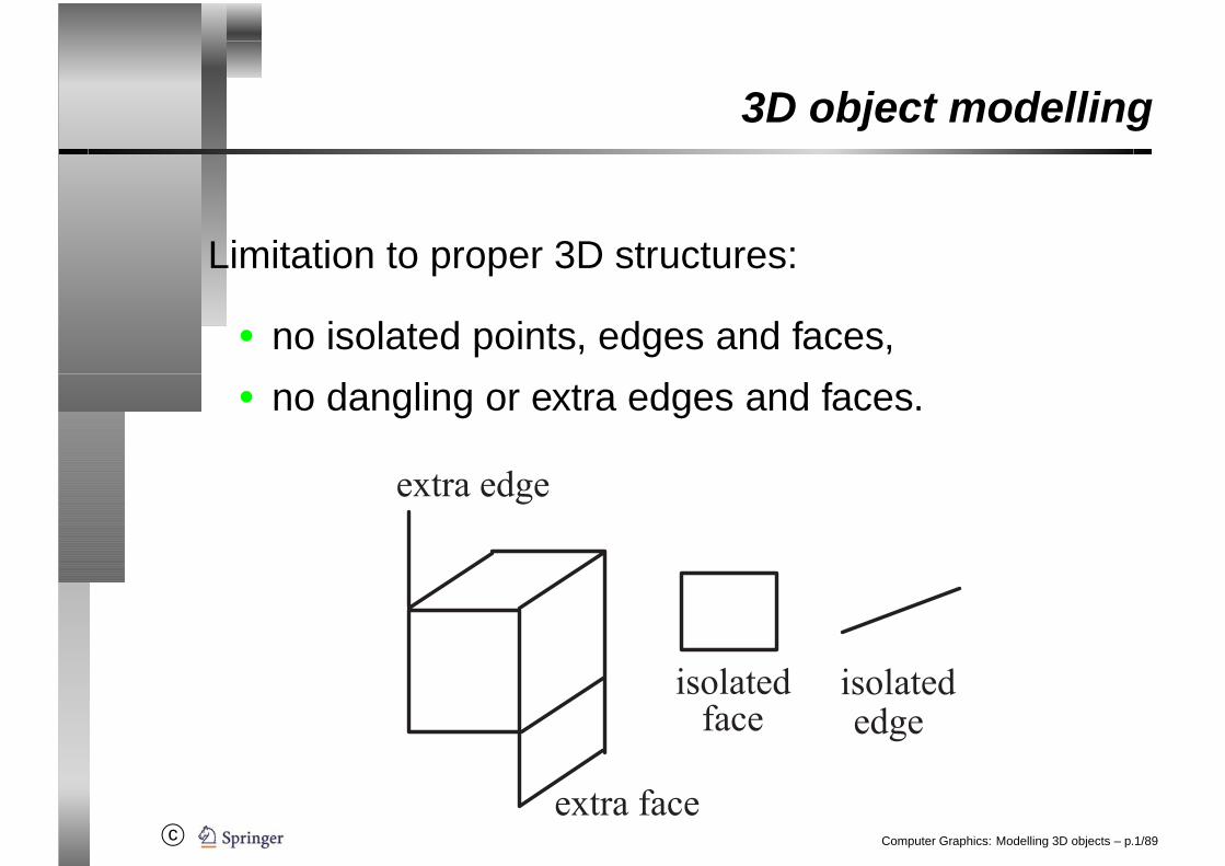
Limitation to proper 3D structures:

• no isolated points, edges and faces,• no dangling or extra edges and faces.

� � � � � � � � � �

� � � � � � � �

� � � � � � � � � � � � � � � � � � � �

Computer Graphics: Modelling 3D objects – p.1/89

c©

Polygons as surface elements

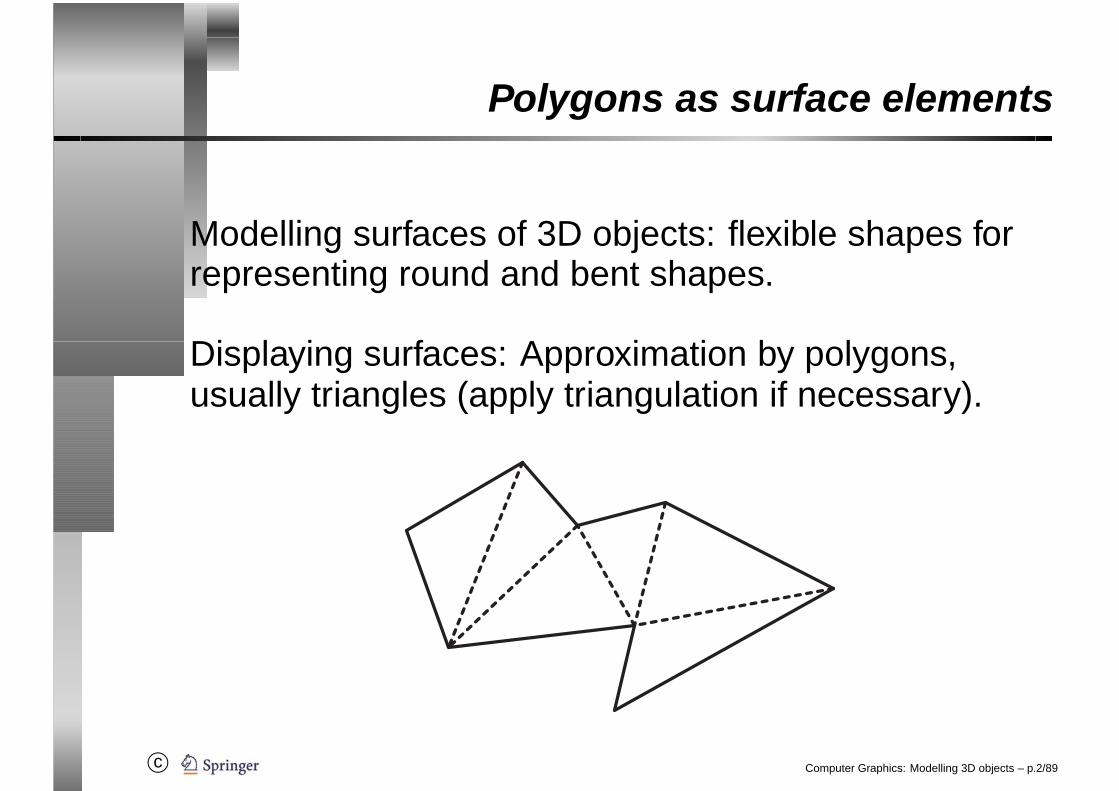
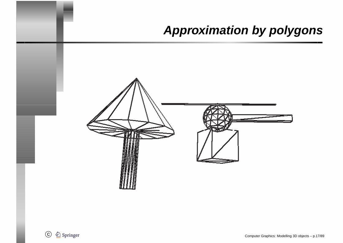
Modelling surfaces of 3D objects: flexible shapes forrepresenting round and bent shapes.

Displaying surfaces: Approximation by polygons,usually triangles (apply triangulation if necessary).


c©

Polygons as surface elements

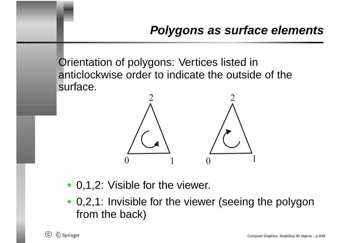
Orientation of polygons: Vertices listed inanticlockwise order to indicate the outside of thesurface.

� �

� �

��

• 0,1,2: Visible for the viewer.• 0,2,1: Invisible for the viewer (seeing the polygon

from the back)


c©

Example: Tetrahedron

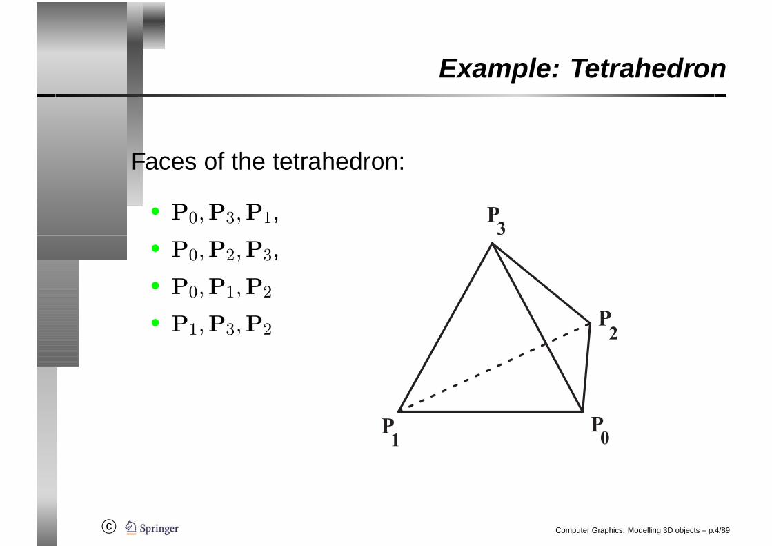
Faces of the tetrahedron:

• P0,P3,P1,• P0,P2,P3,• P0,P1,P2

• P1,P3,P2

��

�

�

��

�

�


c©

Topological notions

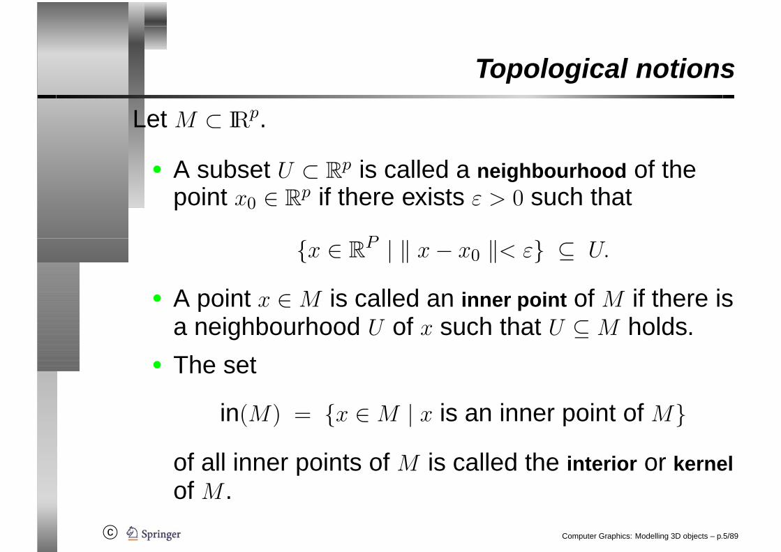
Let M ⊂ IRp.

• A subset U ⊂ Rp is called a neighbourhood of the

point x0 ∈ Rp if there exists ε > 0 such that

{x ∈ RP | ‖ x − x0 ‖< ε} ⊆ U.

• A point x ∈ M is called an inner point of M if there isa neighbourhood U of x such that U ⊆ M holds.

• The set

in(M) = {x ∈ M | x is an inner point of M}of all inner points of M is called the interior or kernelof M .


c©

Topological notions

• A point x is called a boundary point of M if everyneighbourhood of x has nonempty intersectionswith M as well as with the complement of M .

• The set

bound(M) = {x ∈ M | x is a boundary point of M}of all boundary points of M is called the boundaryof M .

• in(M) = M\bound(M).

• M is called an open set if M coincides with itsinterior, i.e., if in(M) = M holds.


c©

Topological notions

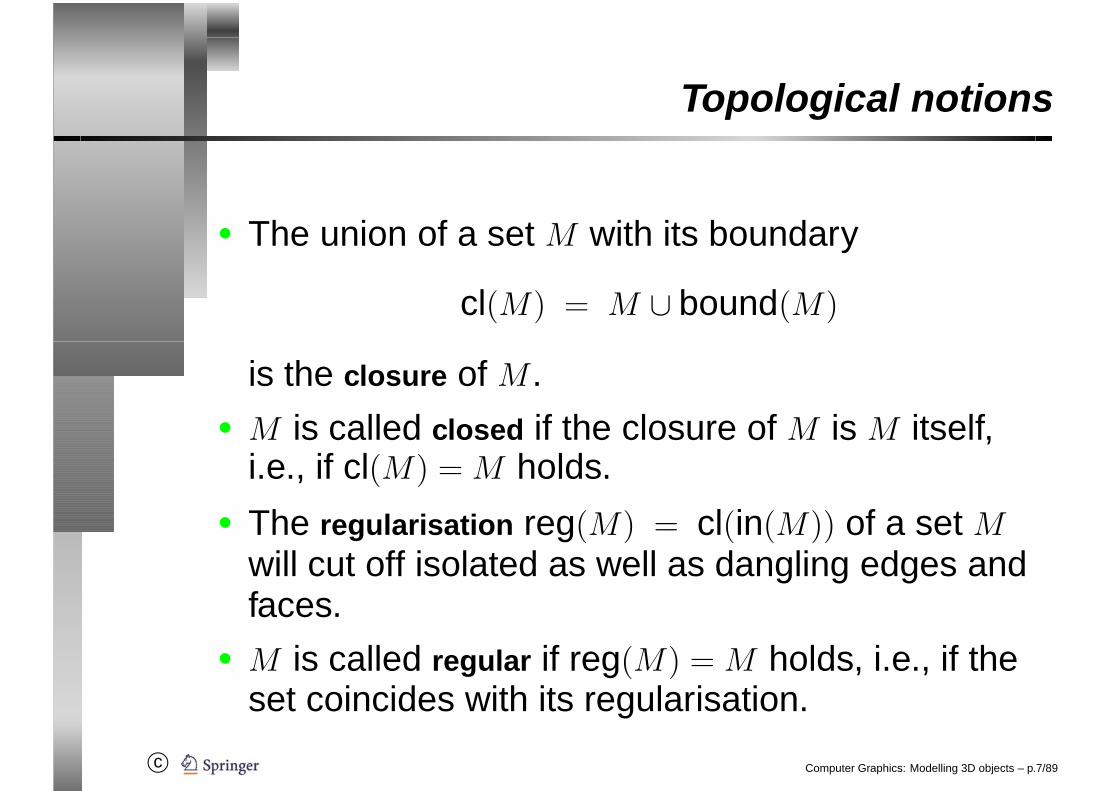
• The union of a set M with its boundary

cl(M) = M ∪ bound(M)

is the closure of M .• M is called closed if the closure of M is M itself,

i.e., if cl(M) = M holds.• The regularisation reg(M) = cl(in(M)) of a set M

will cut off isolated as well as dangling edges andfaces.

• M is called regular if reg(M) = M holds, i.e., if theset coincides with its regularisation.


c©

3D object modelling

� � � � � � � � � � � � � � � � � � � � � � � � � � � � � � � � � � � � � � � � � �

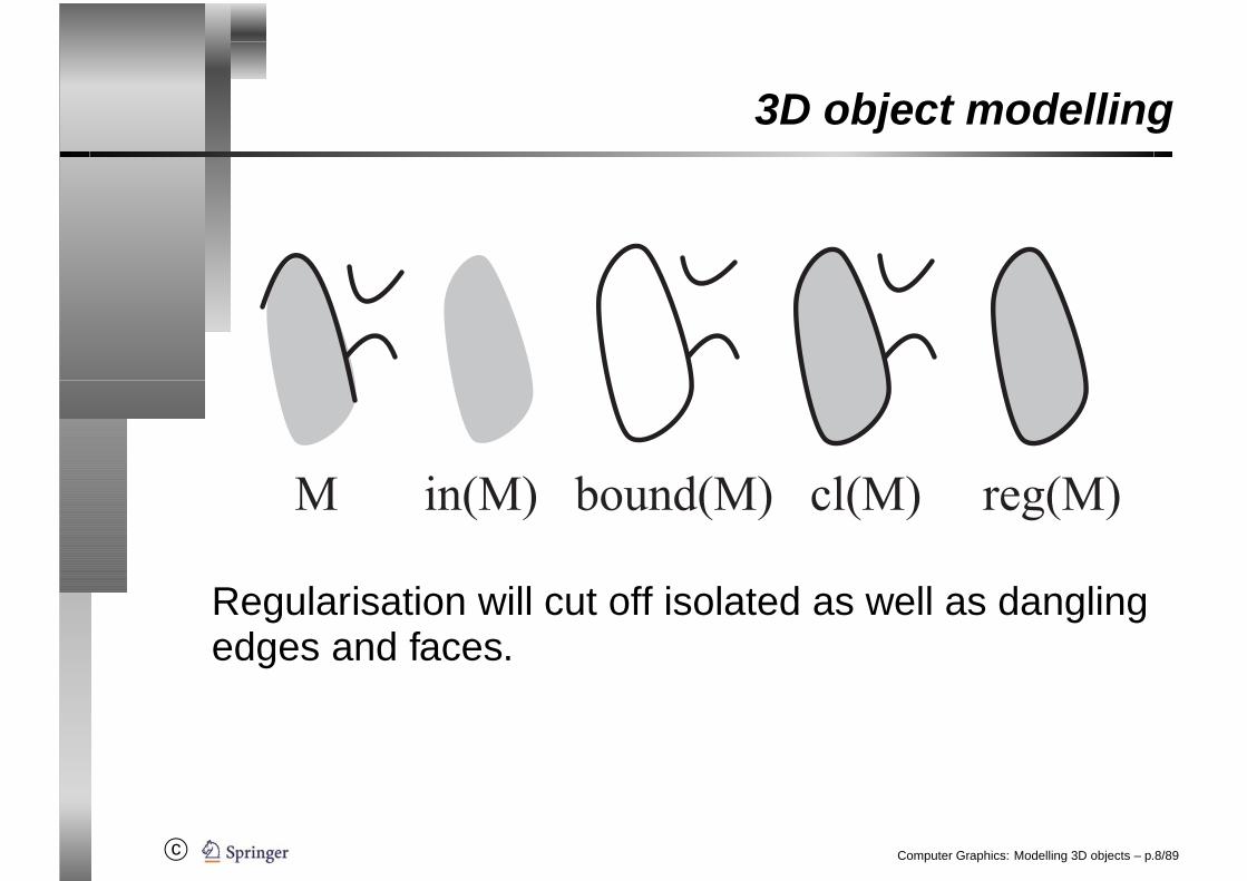
Regularisation will cut off isolated as well as danglingedges and faces.


c©

Voxel model

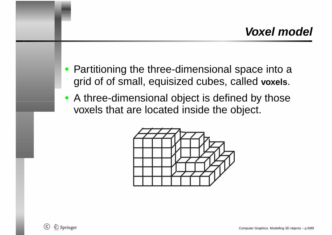
• Partitioning the three-dimensional space into agrid of of small, equisized cubes, called voxels.

• A three-dimensional object is defined by thosevoxels that are located inside the object.


c©

Voxel model

• A voxel belongs to a 3D object if its centre liesinside the 3D object.

• The quality of approximation of a 3D object byvoxels depends on the size of the voxels.

• Small voxels → Good approximation, but highcomputational and memory costs.

• Larger voxels → Rough approximation, but lowcomputational and memory costs.

• Store the 3D object as• a 3D binary matrix or• list of voxels.


c©

Octrees

• Fit the 3D object into a sufficiently large cube orbox.

• Partition the cube into eight smaller cubes.• Smaller cubes that lie completely inside or

completely outside the object are marked with inand off, respectively. No need for furtherrefinement.

• The other cubes are marked with on, indicating thatthe cube intersects the surface of the object. Thecubes are further refined in the same way.


c©

Octrees

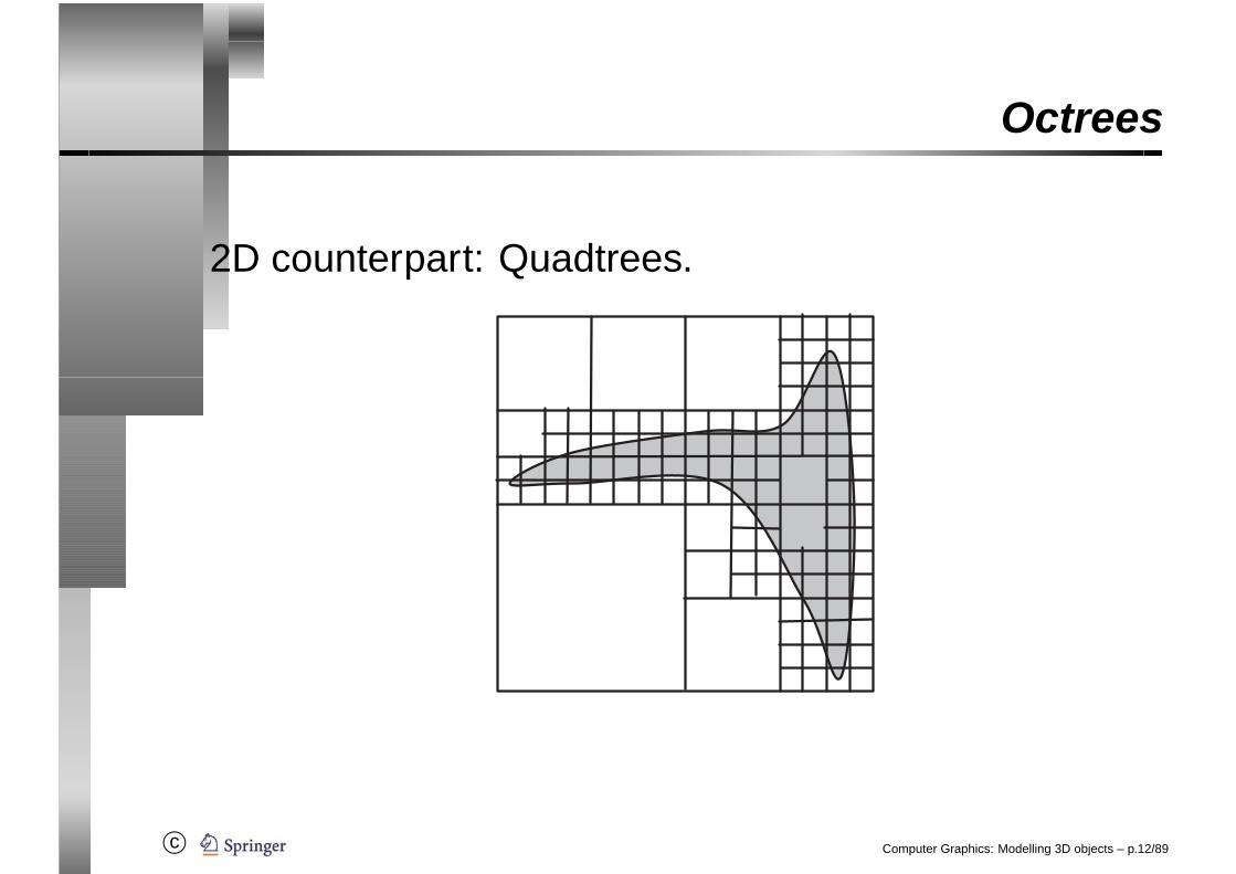
2D counterpart: Quadtrees.


c©

Octrees

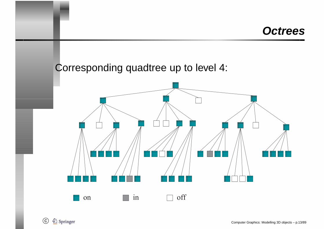
Corresponding quadtree up to level 4:

� � �


c©

CSG scheme

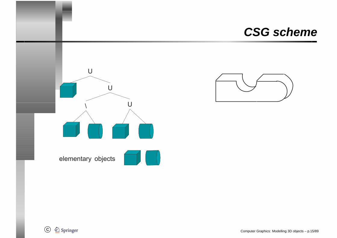
CSG: Constructive solid geometry

Similar to the use of the class Area in Java 2D:

• Collection of elementary geometric objects.(likebox, sphere, cylinder, cone,. . .).

• Transformations and regularised set-theoreticoperations can be applied to these objects toconstruct more complex objects.


c©

CSG scheme

�

� �

�

� � � � � � � � � � � � � �


c©

Sweep representation

A three-dimensional object is generated from atwo-dimensional shape that is moved along atrajectory.

� �

� �


c©

Approximation by polygons


c©

Approximation by polygons

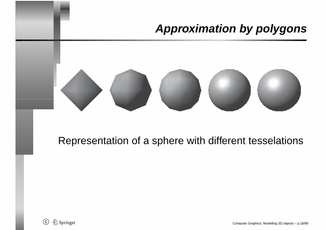
Representation of a sphere with different tesselations


c©

Tesselation in Java 3D

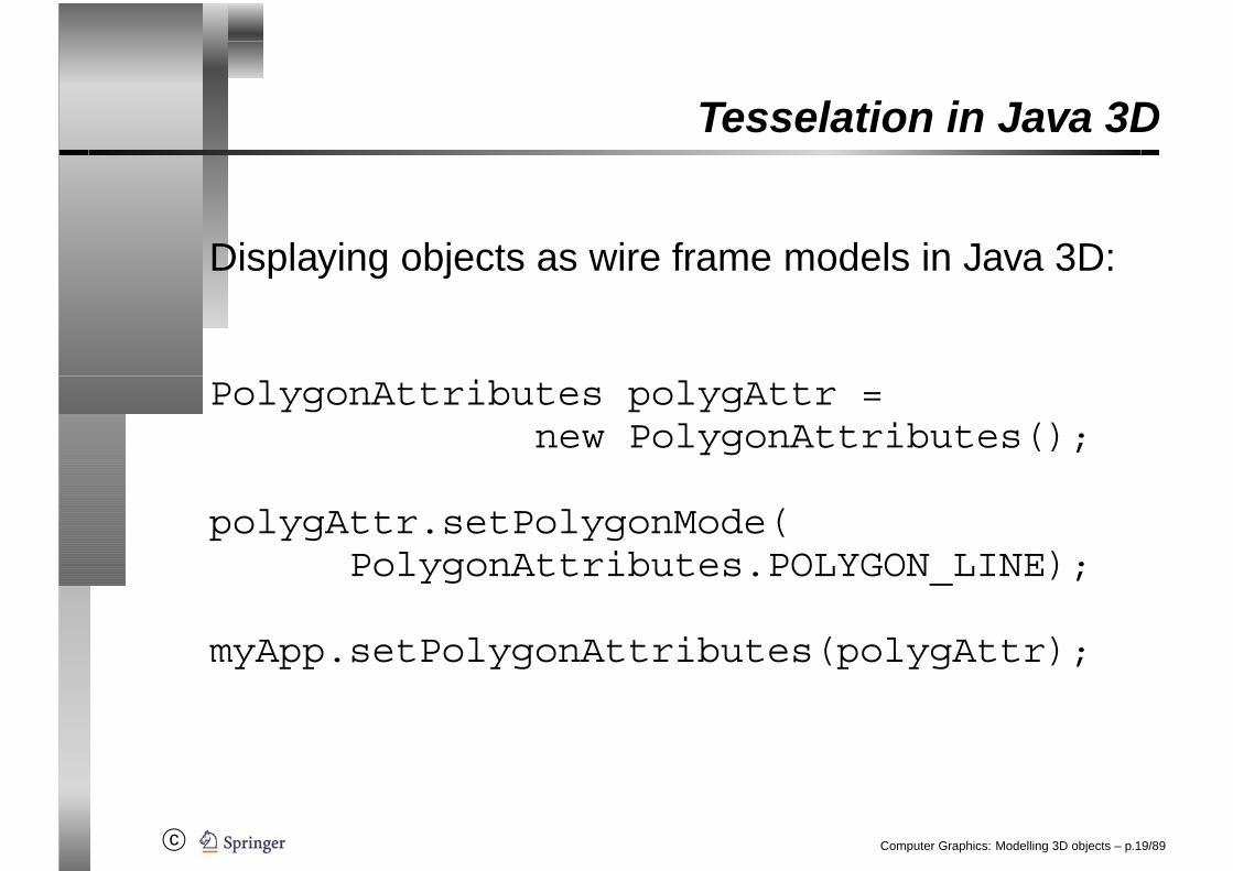
Displaying objects as wire frame models in Java 3D:

PolygonAttributes polygAttr =new PolygonAttributes();

polygAttr.setPolygonMode(PolygonAttributes.POLYGON_LINE);

myApp.setPolygonAttributes(polygAttr);


c©


Specifying the resolution for elementary geometricobjects:

Sphere s = new Sphere(r,Sphere.GENERATE_NORMALS,res,sphereApp);

Approximation of the sphere’s surface by res trianglesat the circumference.


c©


Cylinder c = new Cylinder(r,h,Cylinder.GENERATE_NORMALS,xres,yres,app);

Cone c = new Cone(r,h,Cone.GENERATE_NORMALS,xres,yres,app);

For the approximation of the surfaces, xres trianglesare used around the circumference and yres trianglesalong the height.


c©

Java 3D: GeometryArrays

A GeometryArray defines a 3D object (i.e. itssurface) and mainly consists of

• points (vertices),• faces (or polygons, usually triangles or

quadrangles) defined via the specified vertices,• information about colour or texture,• normal vector containing information about the

true structure of the surface.


c©


A simple way to generate a GeometryArray:

• Partition the surface to be modelled into triangles.• Define an array containing the vertices of the

triangles.

Point3f[] vertices ={new Point3f(...),...new Point3f(...)

};


c©


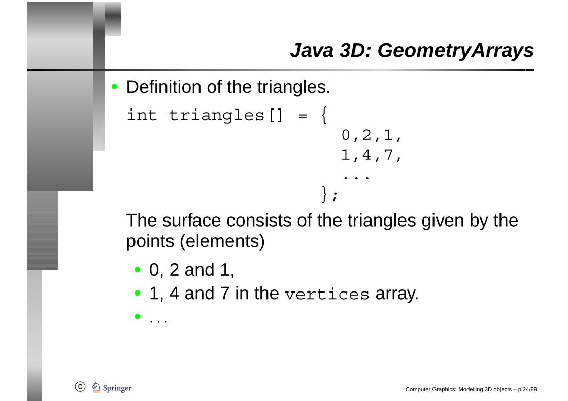
• Definition of the triangles.

int triangles[] = {0,2,1,1,4,7,...

};

The surface consists of the triangles given by thepoints (elements)• 0, 2 and 1,• 1, 4 and 7 in the vertices array.• . . .


c©


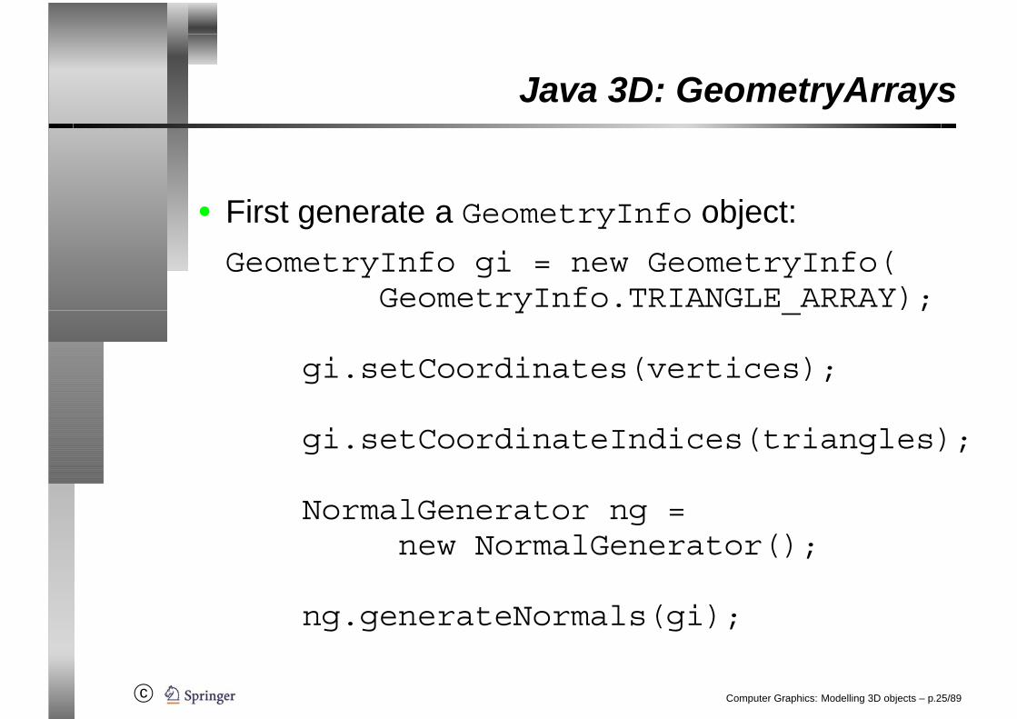
• First generate a GeometryInfo object:

GeometryInfo gi = new GeometryInfo(GeometryInfo.TRIANGLE_ARRAY);

gi.setCoordinates(vertices);

gi.setCoordinateIndices(triangles);

NormalGenerator ng =new NormalGenerator();

ng.generateNormals(gi);


c©


• Generate an GeometryArray from theGeometryInfo object and turn this into aShape3D.

GeometryArray ge = gi.getGeometryArray();

Shape3D inducedShape =new Shape3D(ge,desiredAppearance);

• This Shape3D object can be assigned totransformation groups in the same way aselementary geometric objects.

(see GeomArrayExample.java)


c©

Loading a scene

Java 3D allows to import scenes in various graphicsformats.

Example: Wavefront Object format ( .obj )

This file format contains similar information asGeometryArrays.

Apart from importing some required packages, ascene can be loaded in the following way.


c©

Loading a scene

ObjectFile f = new ObjectFile(ObjectFile.RESIZE);

Scene s = null;

try{

s = f.load("file.obj");}catch (Exception e){

System.out.println("Error ...");}

BranchGroup theScene = s.getSceneGroup();


c©

Loading a scene

The names of the objects contained in this scene areobtained in the following way.

Hashtable sObs = s.getNamedObjects();

Enumeration enum = sObs.keys();

String name;

while (enum.hasMoreElements()){

name = (String) enum.nextElement()System.out.println("Name: "+name);

}


c©

Loading a scene

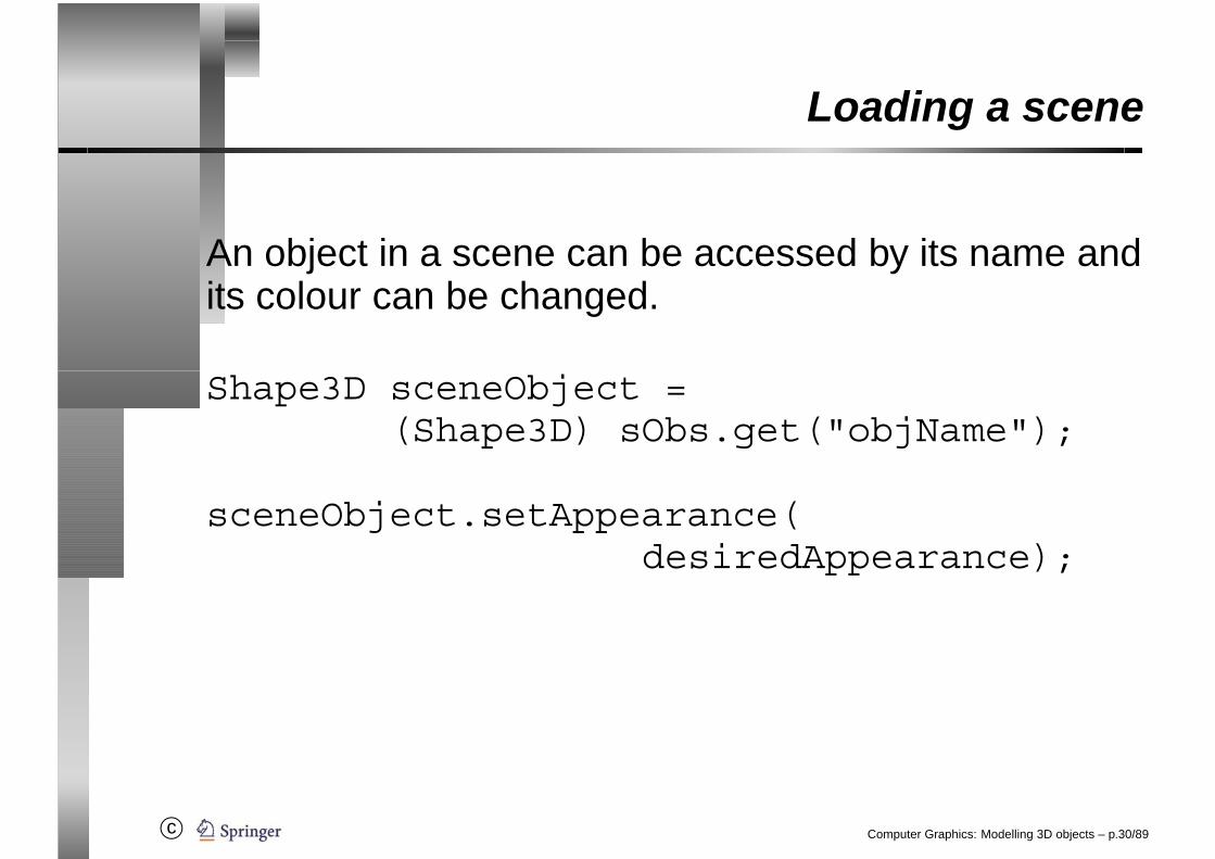
An object in a scene can be accessed by its name andits colour can be changed.

Shape3D sceneObject =(Shape3D) sObs.get("objName");

sceneObject.setAppearance(desiredAppearance);


c©

Loading a scene

Using only a part of a loaded scene.

Shape3D part = (Shape3D)namedObjects.get("partName");

Shape3D extractedPart = (Shape3D)part.cloneTree();

extractedPart.setAppearance(app);tg.addChild(extractedPart);

(see Load3DExample.java andExtract3DExample.java)


c©

Surfaces as functions

another way to define a surface: function in twovariables in implicit form:

F (x, y, z) = 0

Disadvantages:

• Difficult to find an equation that models the desiredsurface.

• The equation needs to be solved for rendering


c©


simpler solution: Description of a surface as a functionin explicit form

z = f(x, y).

Disadvantage: Closed surfaces must be definedpiecewise.


c©


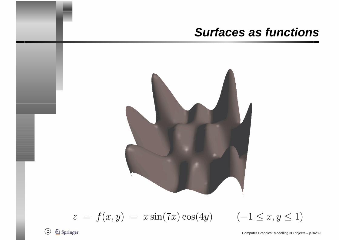
z = f(x, y) = x sin(7x) cos(4y) (−1 ≤ x, y ≤ 1)


c©


Determining the triangles for the representation of thefunction:

�x��

��

��

��y

�z

��

��

��

��

��

��

��

��

��

��

��

��

xi xi+1

yj

yj+1

��

��

��f(xi, yj) �f(xi+1, yj)

�f(xi, yj+1)�f(xi+1, yj+1)


c©


Choosing the resolution (tesselation) for the triangles:

• high resolution: good approximation of thefunction, but high computational costs.

• low resolution: bad approximation of the function,but low computational costs.


c©


possible solution:

variable resolution

In each square the approximation error is computed.Each square is recursively divided into smallersquares until the approximation error is small enoughor a minimum size of the squares is reached.


c©


Landscapes consist of height and texture information.

The height information corresponds to sampling afunction z = f(x, y) where z is the height of thelandscape at the point (x, y).

Problem: Ein narrow grid with height information leadsto a large number of triangles to be rendered, even forthose parts of the landscape that are far away from theviewer.


c©

Level of Detail (LOD)

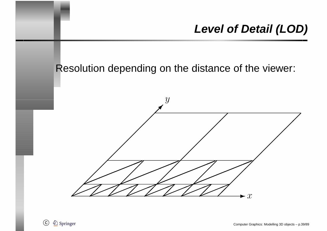
Resolution depending on the distance of the viewer:

� x��

��

��

��

��

��y

��

�

��

��

�

��

�

��

�

��

��

��

��

��

��


c©

Text

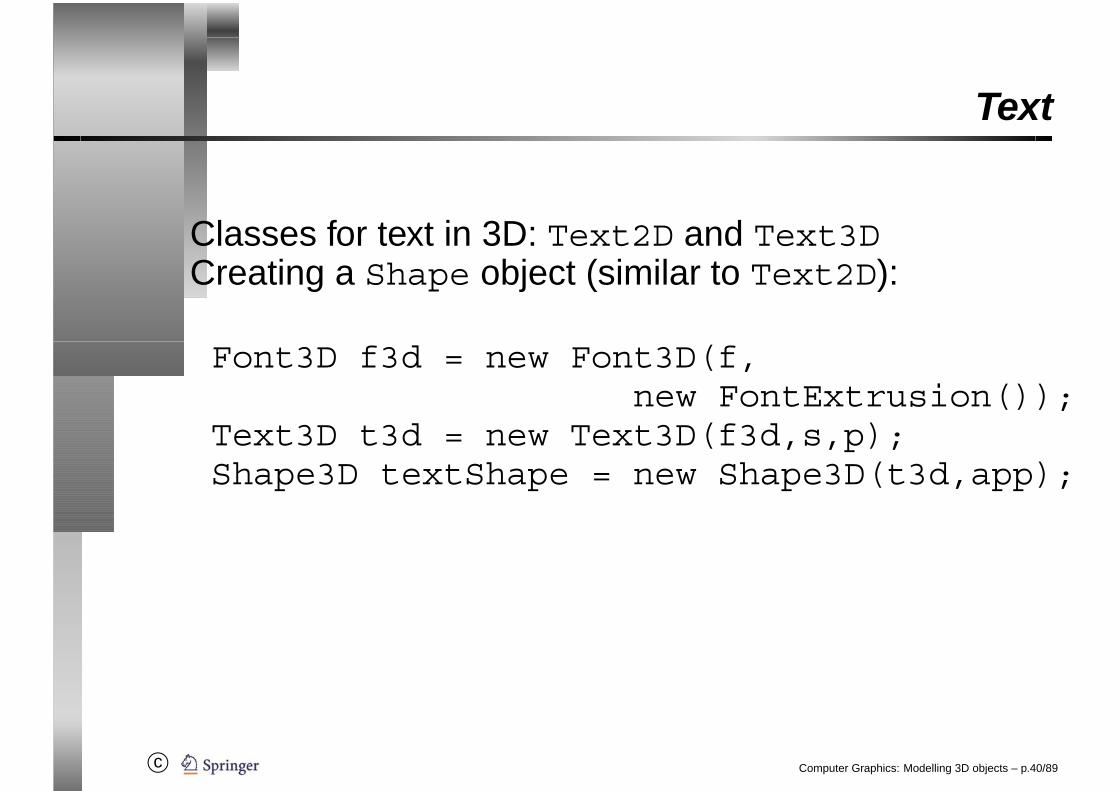
Classes for text in 3D: Text2D and Text3DCreating a Shape object (similar to Text2D):

Font3D f3d = new Font3D(f,new FontExtrusion());

Text3D t3d = new Text3D(f3d,s,p);Shape3D textShape = new Shape3D(t3d,app);


c©

Billboard Behaviour

For text as legend it is important that the text is alwaysoriented to the viewer. This is called Billboard Behaviour.

Billboard bb = new Billboard(tgBBGroup,Billboard.ROTATE_ABOUT_POINT,

p);bb.setSchedulingBounds(bounds);tgBBGroup.addChild(bb);tgBBGroup.setCapability(

TransformGroup.ALLOW_TRANSFORM_WRITE);


c©

Surface modelling

• Round or bent surfaces are usually approximatedby a sufficiently large number of small triangles.

• For modelling surfaces, it is more common to usefreeform surfaces, especially for CAD applications.

• From a freeform surface model, differentapproximations by triangles can be generated,depending on the desired precision or on thedistance of the viewer to the object (LOD: level ofdetail).


c©

Surface modelling

• Normal vectors to surfaces are needed for shadingeffects (and also for elimination of invisiblesurfaces).

• The normal vectors for the triangles are taken asthe normal vectors to the planar polygons that thetriangles represent, but as normal vectors to theoriginal bent surface.

• Methods for computing normal vectors will beintroduced later on.


c©

Parametric curves and surfaces

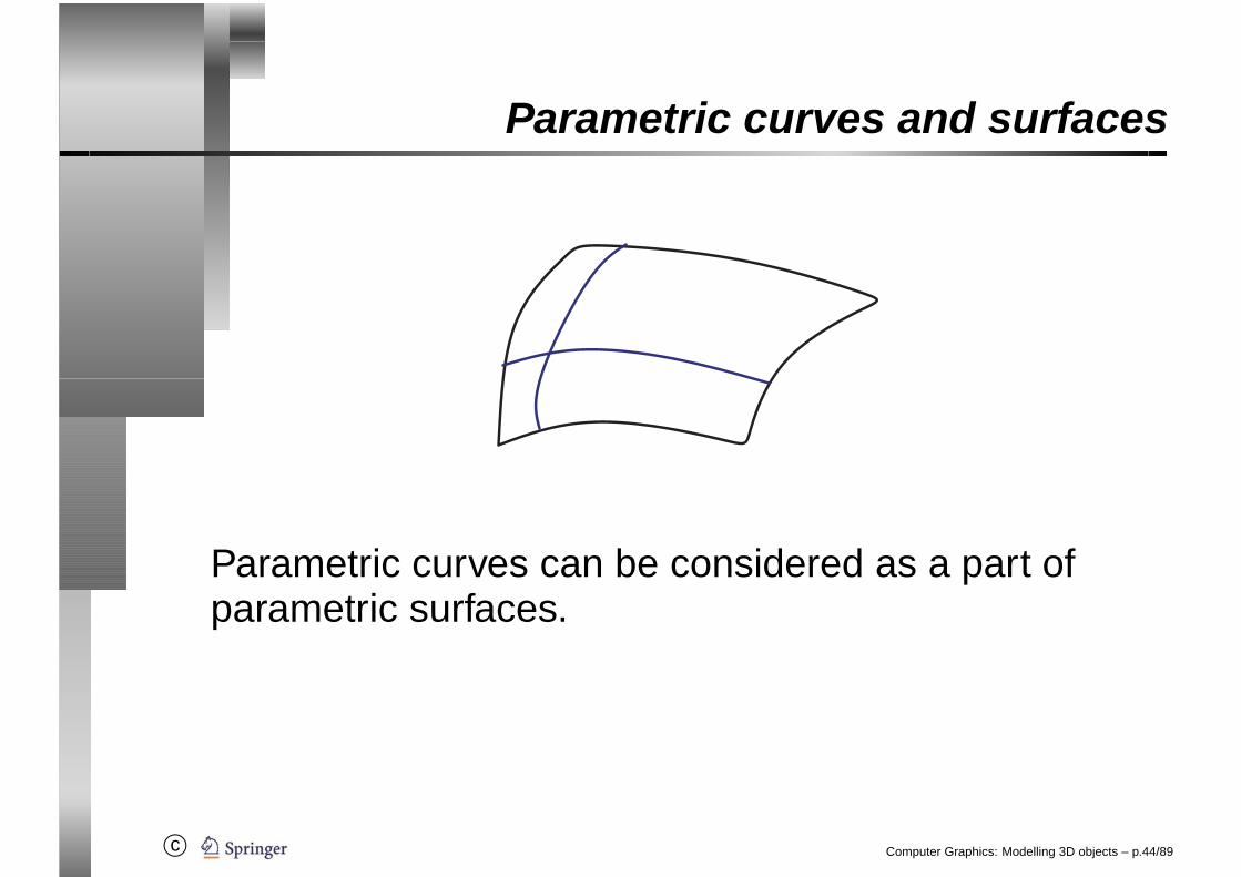
Parametric curves can be considered as a part ofparametric surfaces.


c©

Parametric curves

Parametric surfaces are defined on the basis ofparametric curves (similar to QuadCurve2D orCubicCurve2D in Java 2D).

Parametric curves are defined via points (in 3Dspace), so-called control points.

Interpolation refers to curves that pass through allcontrol points.

Approximation only requires that the curve gets closeto the control points, but it does not have to passthrough them.


c©

Modelling curves

When curves (or also surfaces) are defined via a setof parameters (f.e. points in 3D space), the followingproperties will make modelling and adjusting suchcurves easier.

Controllability: The influence of the parameters on theshape of the curve can be understood in anintuitive way. When the shape of a curve has to bechanged, it should be clear for the user whichparameters he should modify in which way in orderto achieve the desired change.


c©

Modelling curves

Locality principle: It must be possible to carry out localchanges on the curve. Modifying one control pointshould only change the curve in theneighbourhood of this control point and not alterthe curve completely.

Smoothness: The curve should satisfy certainsmoothness properties. It should not only becontinuous without jumps, it should have no sharpbends. The latter property requires the curve to bedifferentiable. In some cases it is even necessarythat higher derivatives exist. It also desirable thatthe curve is of bounded variation. This means itshould stay somehow close to its control points.


c©

Interpolation with polynomials

Given (n + 1) control points, there is always aninterpolation polynomial of degree n or less thatpasses exactly through the control points.

Disadvantages:

• For a larger number of points, the polynomial willhave a high degree leading to high computationalcosts.

• Interpolation polynomials do not satisfy the localityprinciple.


c©


Disadvantages:

• Clipping for such polynomials is also not easy,since a polynomial interpolating a given set ofcontrol points can deviate arbitrarily from theregion around the control points.

• Polynomials of high degree tend to oscillatebetween the control points.


c©


-1.5

-1

-0.5

0

0.5

1

1.5

0 1 2 3 4 5

f(x)

Interpolation polynomial of degree 5 passing throughthe control points (0,0), (1,0), (2,0), (3,0), (4,1), (5,0):

f(x) =1

24· (−x5 + 11x4 − 41x3 + 61x2 + 30x

)Computer Graphics: Modelling 3D objects – p.50/89

c©


-1.5

-1

-0.5

0

0.5

1

1.5

0 1 2 3 4 5

f(x)

The interpolation polynomial does not stay within theconvex hull of the control points.


c©

Bézier curves

i-th Bernstein polynomial of degree n (i ∈ {0, . . . , n}):

B(n)i (t) =

(n

i

)· (1 − t)n−i · ti (t ∈ [0, 1])

Properties:

B(n)i (t) ∈ [0, 1] for all t ∈ [0, 1],

n∑i=0

B(n)i (t) = 1 for all t ∈ [0, 1].


c©

Bézier curves

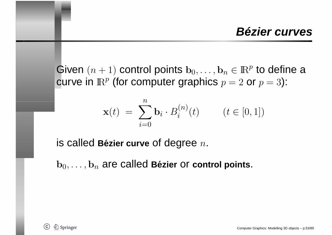
Given (n + 1) control points b0, . . . ,bn ∈ IRp to define acurve in IRp (for computer graphics p = 2 or p = 3):

x(t) =n∑

i=0

bi · B(n)i (t) (t ∈ [0, 1])

is called Bezier curve of degree n.

b0, . . . ,bn are called Bezier or control points.


c©

Bézier curves• x(0) = b0 and x(1) = bn always hold.

The Bézier curve interpolates the first and the lastpoint.

In general, the curve does not pass through theother control points.

• Furthermore:

x(0) = n · (b1 − b0)

x(1) = n · (bn − bn−1)

The tangent vector in the first point b0 points in thedirection of the point b1 and the tangent vector inthe last point bn points in the direction of the pointbn−1.


c©

Bézier curves

• Due to the properties of the Bernstein polynomials,the Bézier curve is everywhere a convexcombination of the control points.

The Bézier curve stays within the convex hull ofthe control points.

• Bézier curves are invariant under affinetransformations.

When an affine transformation is applied to thecontrol points, the resulting Bézier curve withrespect to the new control points coincides withthe transformed Bézier curve.


c©

Bézier curves• Bézier curves are symmetric w.r.t. the control

points, i.e. the control points b0, . . . ,bn andbn, . . . ,b0 lead to the same curve. The curve isonly passed through in the reverse direction.

• Using a convex combination of control points oftwo sets of control points, the resulting Béziercurve is the convex combination of the twocorresponding Bézier curves.

• b0, . . . , bn defines the Bézier curve x(t).• b0, . . . , bn defines the Bézier curve x(t).• αb0 + βb0, . . . , αbn + βbn defines the Bézier

curve x(t) = αx(t) + βx(t), given α + β = 1,α, β ≥ 0.


c©

Bézier curves

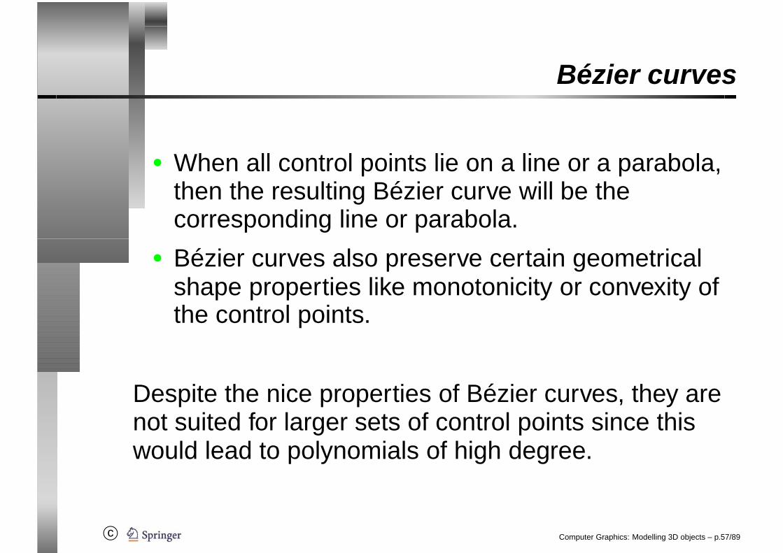
• When all control points lie on a line or a parabola,then the resulting Bézier curve will be thecorresponding line or parabola.

• Bézier curves also preserve certain geometricalshape properties like monotonicity or convexity ofthe control points.

Despite the nice properties of Bézier curves, they arenot suited for larger sets of control points since thiswould lead to polynomials of high degree.


c©

B-splines

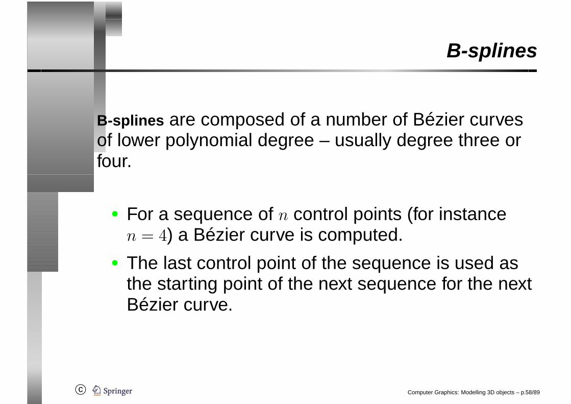
B-splines are composed of a number of Bézier curvesof lower polynomial degree – usually degree three orfour.

• For a sequence of n control points (for instancen = 4) a Bézier curve is computed.

• The last control point of the sequence is used asthe starting point of the next sequence for the nextBézier curve.


c©

B-splines

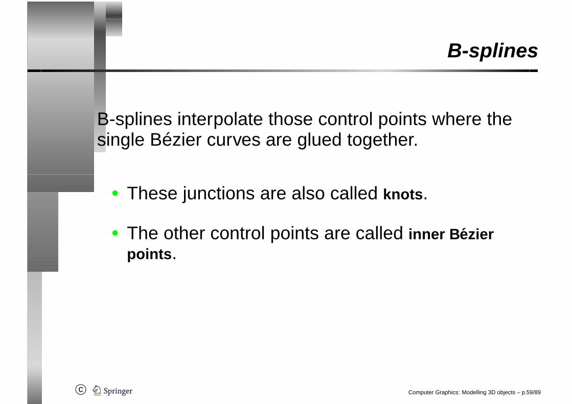
B-splines interpolate those control points where thesingle Bézier curves are glued together.

• These junctions are also called knots.

• The other control points are called inner Bezierpoints.


c©

B-splines

P P

P P

1

4

P6

7

3

P2

P5

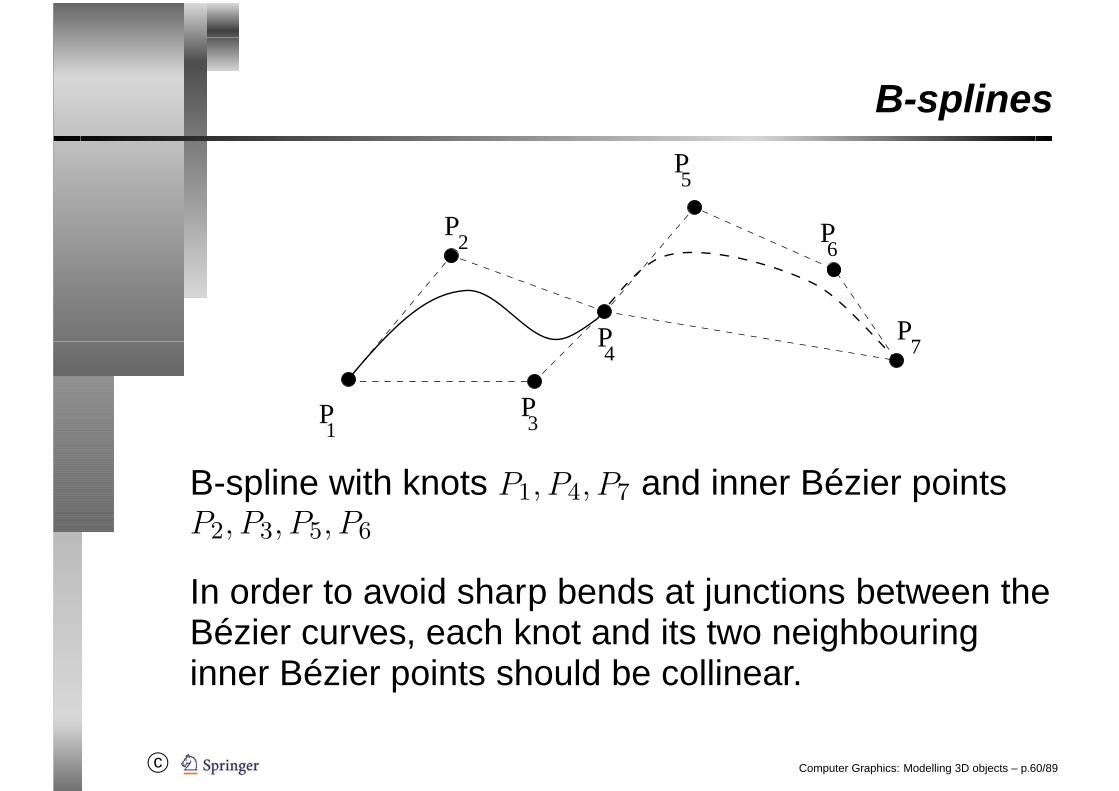
B-spline with knots P1, P4, P7 and inner Bézier pointsP2, P3, P5, P6

In order to avoid sharp bends at junctions between theBézier curves, each knot and its two neighbouringinner Bézier points should be collinear.


c©

B-splines

By choosing the inner Bézier points properly, aB-spline of degree n can be differentiated (n− 1) times.

Cubic B-splines are based on polynomials of degreethree and can therefore be twice differential when theinner Bézier points are chosen correctly.


c©

B-splines

� � ��

�

�

�

�

�

�

�

�

��

�

�


c©

B-splines

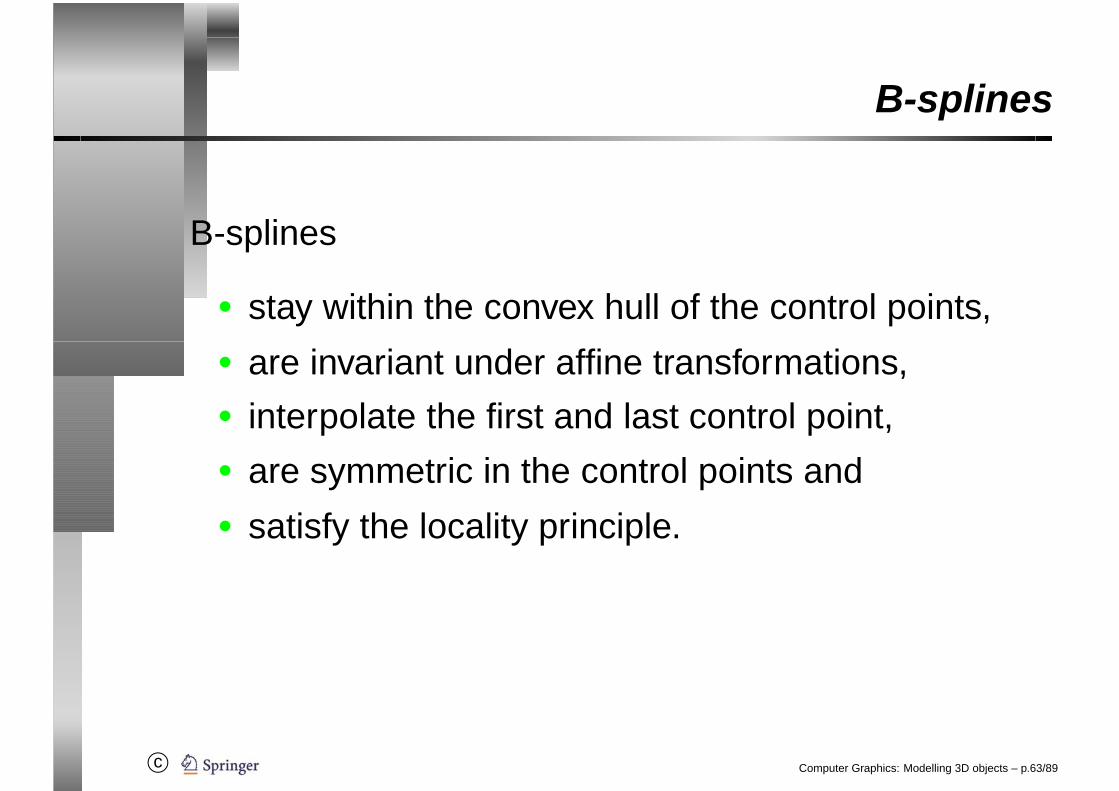
B-splines

• stay within the convex hull of the control points,• are invariant under affine transformations,• interpolate the first and last control point,• are symmetric in the control points and• satisfy the locality principle.


c©

B-splines

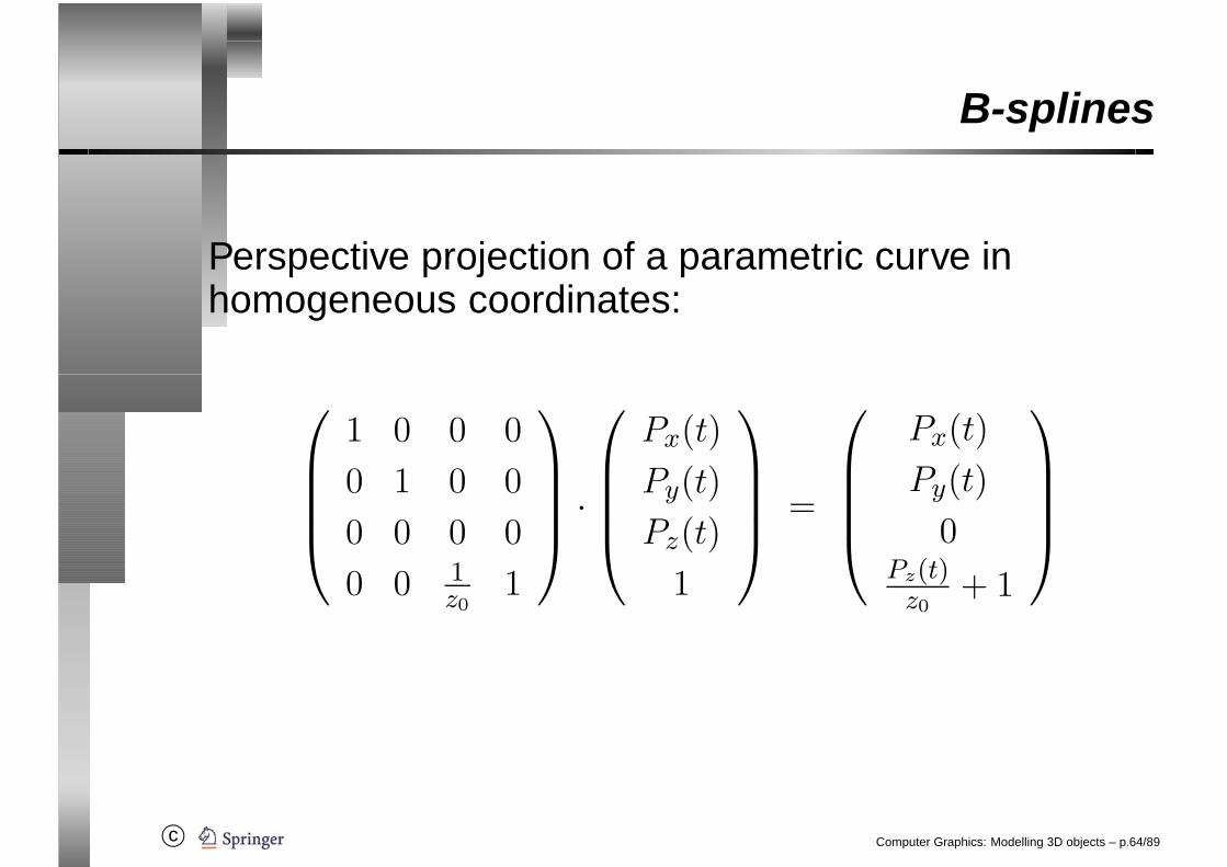
Perspective projection of a parametric curve inhomogeneous coordinates:

⎛⎜⎜⎜⎝

1 0 0 0

0 1 0 0

0 0 0 0

0 0 1z0

1

⎞⎟⎟⎟⎠ ·

⎛⎜⎜⎜⎝

Px(t)

Py(t)

Pz(t)

1

⎞⎟⎟⎟⎠ =

⎛⎜⎜⎜⎝

Px(t)

Py(t)

0Pz(t)

z0+ 1

⎞⎟⎟⎟⎠


c©

B-splines

In Cartesian coordinates:

⎛⎜⎜⎜⎜⎜⎝

Px(t)Pz(t)

z0+1

Px(t)Pz(t)

z0+1

0

⎞⎟⎟⎟⎟⎟⎠

Result: Rational function in t.


c©

NURBS

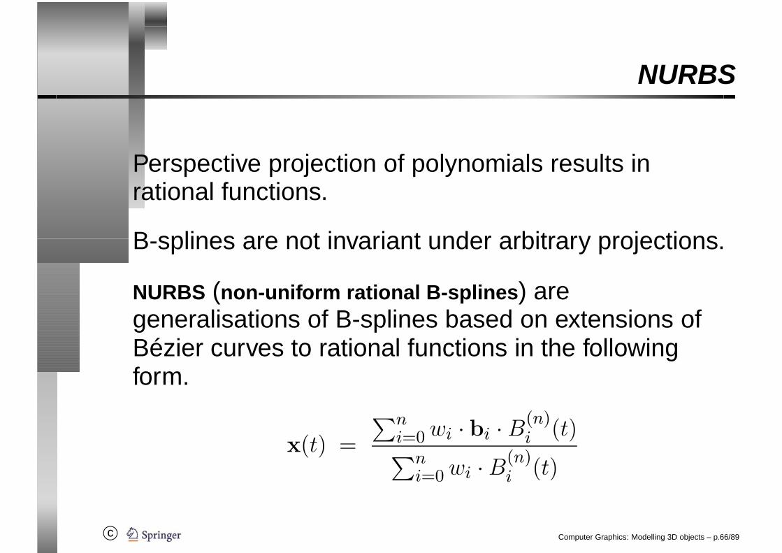
Perspective projection of polynomials results inrational functions.

B-splines are not invariant under arbitrary projections.

NURBS (non-uniform rational B-splines) aregeneralisations of B-splines based on extensions ofBézier curves to rational functions in the followingform.

x(t) =

∑ni=0 wi · bi · B(n)

i (t)∑ni=0 wi · B(n)

i (t)


c©

Efficient polynomial evaluation

In order to draw a parametric curve (or surface),polynomials, usually of degree 3, have to beevaluated.

For drawing a cubic curve, the parametric curve isevaluated at equidistant values of the parameter t.

The corresponding points are computed andconnected by line segments.


c©


Scheme of forward differences δ > 0:

∆f(t) = f(t + δ) − f(t)

i.e.f(t + δ) = f(t) + ∆f(t)

orfn+1 = fn + ∆fn

For f(t) = at3 + bt2 + ct + d, this leads to

∆f(t) = 3at2δ + t(3aδ2 + 2bδ) + aδ3 + bδ2 + cδ.


c©


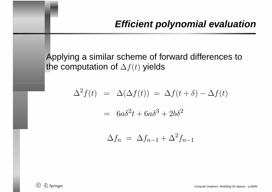
Applying a similar scheme of forward differences tothe computation of ∆f(t) yields

∆2f(t) = ∆(∆f(t)) = ∆f(t + δ) − ∆f(t)

= 6aδ2t + 6aδ3 + 2bδ2

∆fn = ∆fn−1 + ∆2fn−1


c©


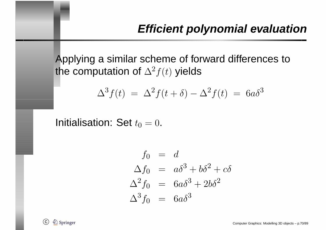
Applying a similar scheme of forward differences tothe computation of ∆2f(t) yields

∆3f(t) = ∆2f(t + δ) − ∆2f(t) = 6aδ3

Initialisation: Set t0 = 0.

f0 = d

∆f0 = aδ3 + bδ2 + cδ

∆2f0 = 6aδ3 + 2bδ2

∆3f0 = 6aδ3


c©


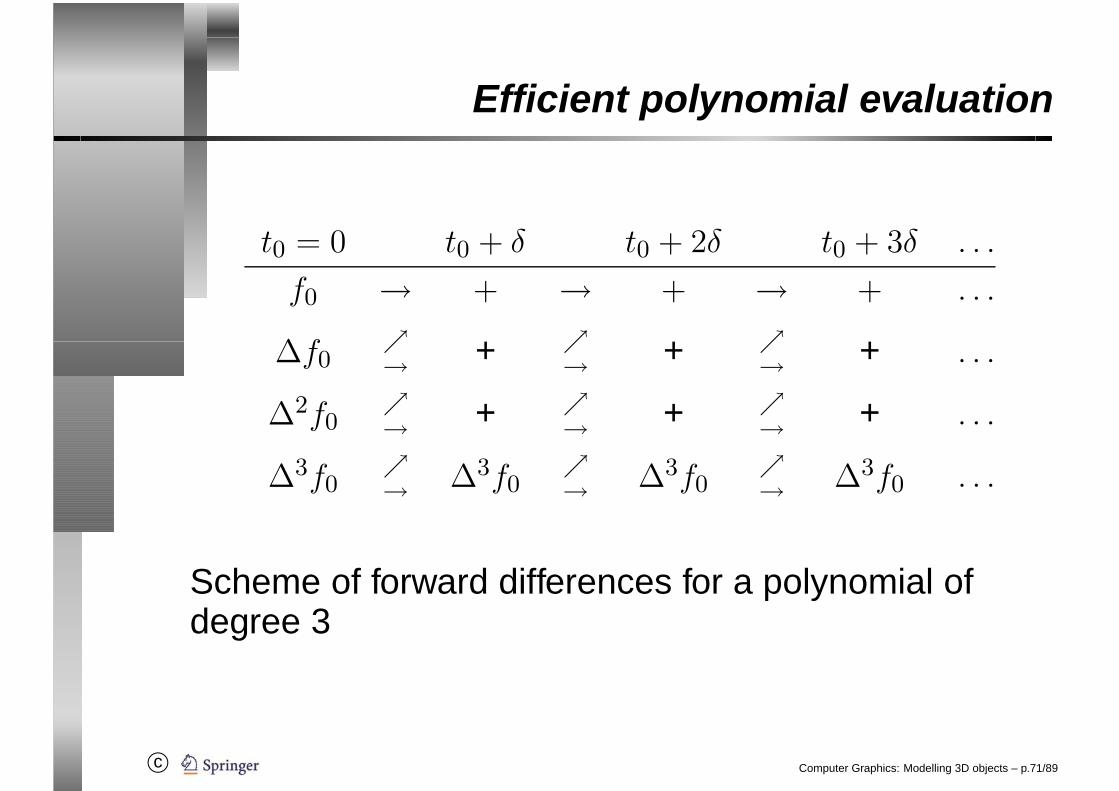
t0 = 0 t0 + δ t0 + 2δ t0 + 3δ . . .

f0 → + → + → + . . .

∆f0↗→ + ↗

→ + ↗→ + . . .

∆2f0↗→ + ↗

→ + ↗→ + . . .

∆3f0↗→ ∆3f0

↗→ ∆3f0

↗→ ∆3f0 . . .

Scheme of forward differences for a polynomial ofdegree 3


c©


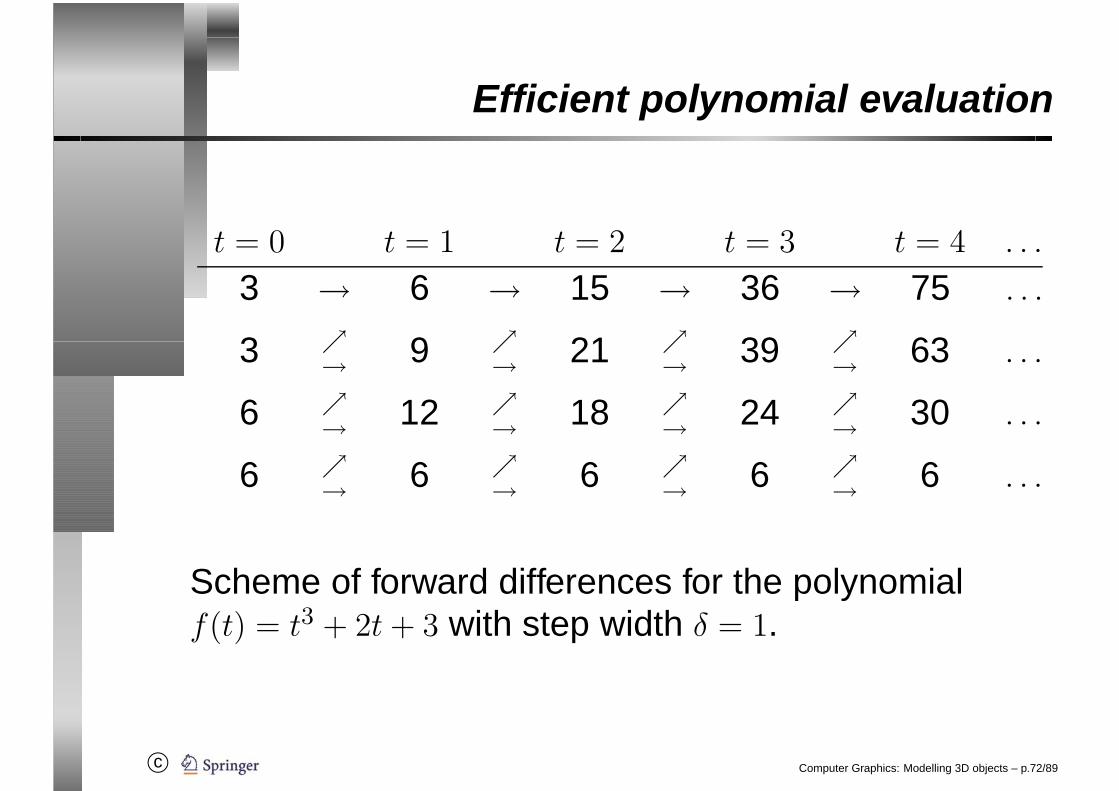
t = 0 t = 1 t = 2 t = 3 t = 4 . . .

3 → 6 → 15 → 36 → 75 . . .

3 ↗→ 9 ↗

→ 21 ↗→ 39 ↗

→ 63 . . .

6 ↗→ 12 ↗

→ 18 ↗→ 24 ↗

→ 30 . . .

6 ↗→ 6 ↗

→ 6 ↗→ 6 ↗

→ 6 . . .

Scheme of forward differences for the polynomialf(t) = t3 + 2t + 3 with step width δ = 1.


c©

Freeform surfaces

s

t

P (t)

P (t)t=0

t=0.2

t=0.4

t=0.6

t=0.8

t=1

1

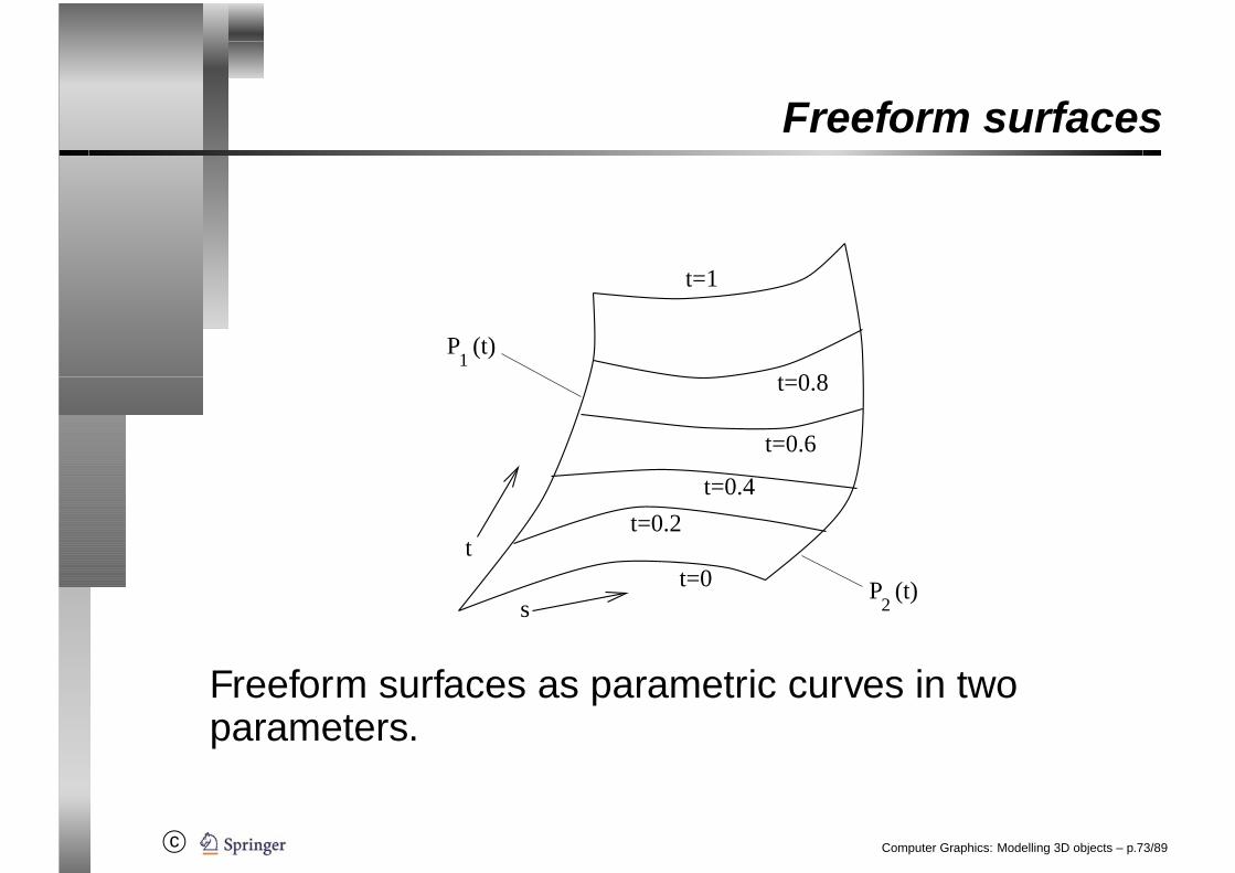
2

Freeform surfaces as parametric curves in twoparameters.


c©

Freeform surfaces

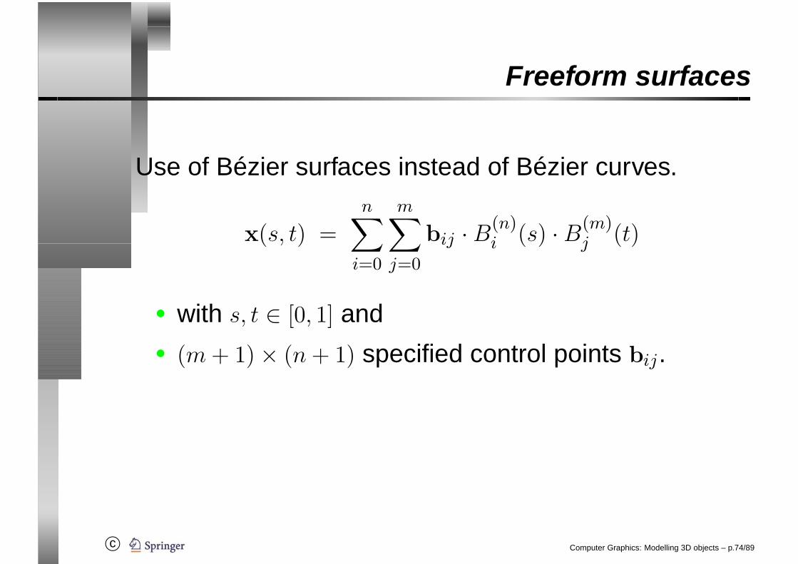
Use of Bézier surfaces instead of Bézier curves.

x(s, t) =n∑

i=0

m∑j=0

bij · B(n)i (s) · B(m)

j (t)

• with s, t ∈ [0, 1] and• (m + 1) × (n + 1) specified control points bij.


c©

Freeform surfaces

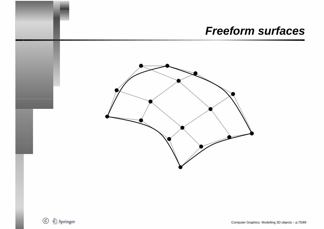
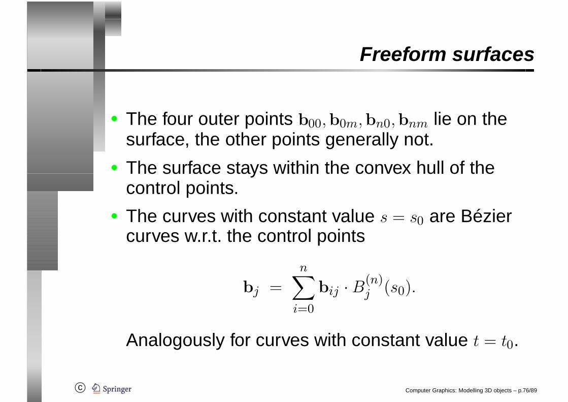
• The four outer points b00,b0m,bn0,bnm lie on thesurface, the other points generally not.

• The surface stays within the convex hull of thecontrol points.

• The curves with constant value s = s0 are Béziercurves w.r.t. the control points

bj =n∑

i=0

bij · B(n)j (s0).

Analogously for curves with constant value t = t0.


c©

Freeform surfaces

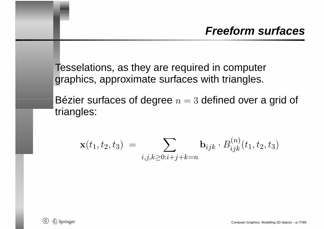
Tesselations, as they are required in computergraphics, approximate surfaces with triangles.

Bézier surfaces of degree n = 3 defined over a grid oftriangles:

x(t1, t2, t3) =∑

i,j,k≥0:i+j+k=n

bijk · B(n)ijk (t1, t2, t3)


c©

Freeform surfaces

with the Bernstein polynomials

B(n)ijk (t1, t2, t3) =

n!

i!j!k!· ti1 · tj2 · tk3

where t1 + t2 + t3 = 1, t1, t2, t3 ≥ 0 and

i + j + k = n, i, j, k ∈ IN.


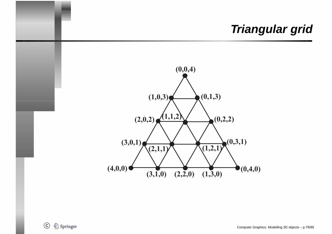
c©

Triangular grid

� � � � � � � � � � � � � � � � � � � � � � � �

� � � � � �

� � � � � �

� � � � � �

� � � � � �

� � � � � �

� � � � � �

� � � � � �

� � � � � �

� � � � � � � � � � � �

� � � � � �


c©

Normal vectors for triangles

Equation of the plane E induced by a triangle:

Ax + By + Cz + D = 0.

The vector (A,B,C) is the (nonnormalised) normalvector to the plane:

Let n = (nx, ny, nz)� (nonnormalised) normal vector.

Let v = (vx, vy, vz)� be a point in the plane E.


c©


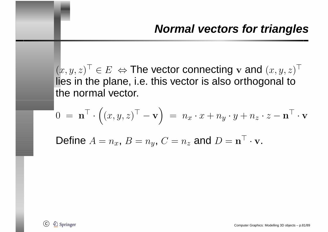
(x, y, z)� ∈ E ⇔ The vector connecting v and (x, y, z)�lies in the plane, i.e. this vector is also orthogonal tothe normal vector.

0 = n� ·((x, y, z)� − v

)= nx · x + ny · y + nz · z − n� · v

Define A = nx, B = ny, C = nz and D = n� · v.


c©


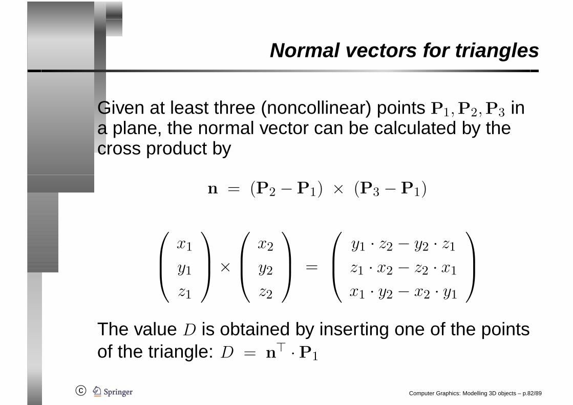
Given at least three (noncollinear) points P1,P2,P3 ina plane, the normal vector can be calculated by thecross product by

n = (P2 − P1) × (P3 − P1)

⎛⎜⎝ x1

y1

z1

⎞⎟⎠×

⎛⎜⎝ x2

y2

z2

⎞⎟⎠ =

⎛⎜⎝ y1 · z2 − y2 · z1

z1 · x2 − z2 · x1

x1 · y2 − x2 · y1

⎞⎟⎠

The value D is obtained by inserting one of the pointsof the triangle: D = n� · P1


c©

Normal vectors for surfaces

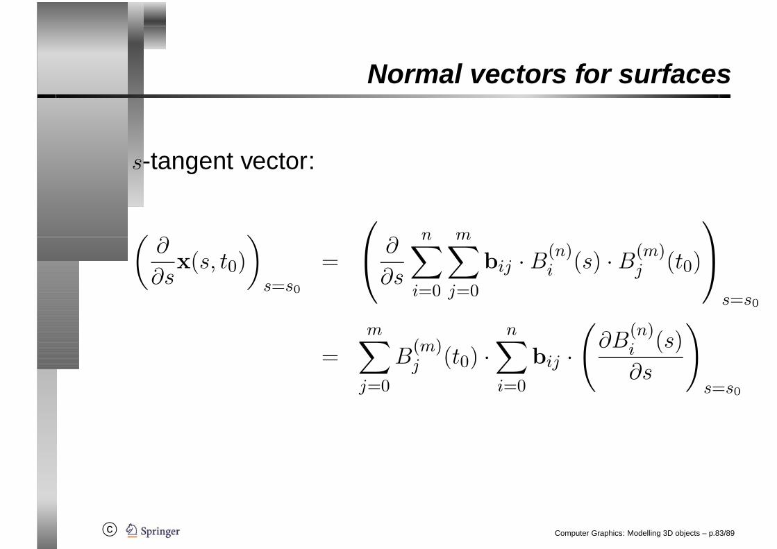
s-tangent vector:

(∂

∂sx(s, t0)

)s=s0

=

⎛⎝ ∂

∂s

n∑i=0

m∑j=0

bij · B(n)i (s) · B(m)

j (t0)

⎞⎠

s=s0

=

m∑j=0

B(m)j (t0) ·

n∑i=0

bij ·(

∂B(n)i (s)

∂s

)s=s0


c©


t-tangent vector:

(∂

∂tx(s0, t)

)t=t0

=

⎛⎝ ∂

∂t

n∑i=0

m∑j=0

bij · B(n)i (s0) · B(m)

j (t)

⎞⎠

t=t0

=n∑

i=0

B(n)i (s0) ·

m∑j=0

bij ·⎛⎝∂B

(m)j (t)

∂t

⎞⎠

t=t0


c©


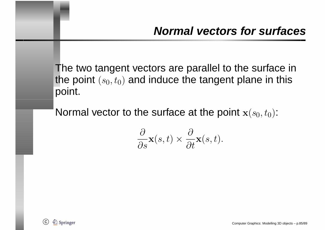
The two tangent vectors are parallel to the surface inthe point (s0, t0) and induce the tangent plane in thispoint.

Normal vector to the surface at the point x(s0, t0):

∂

∂sx(s, t) × ∂

∂tx(s, t).


c©

Varying normal vectors for triangles

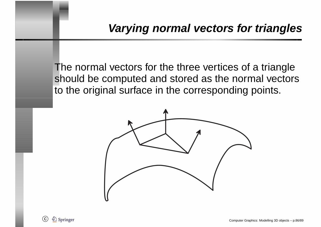
The normal vectors for the three vertices of a triangleshould be computed and stored as the normal vectorsto the original surface in the corresponding points.


c©


When modelling a surface in Java 3D with aGeometryInfo object, the normal vectors will becomputed w.r.t. to the planar triangles.

By setting the crease angle, interpolation of normalvectors of triangles can be enforced.

NormalGenerator ng =new NormalGenerator();

ng.setCreaseAngle(alpha);


c©


The angle alpha specifies how much neighbouringtriangles may deviate from the ideal same plane inorder to apply interpolation of normal vectors.

The default value for alpha is zero (no interpolation).

(see NormalsForGeomArrays.java)


polygons as surface elements - ostfalia public web server

Documents