polling systems with breakdowns and repairs

Stochastics and Statistics

Polling systems with breakdowns and repairs

Oren Nakdimon, Uri Yechiali *

Department of Statistics and Operations Research, School of Mathematical Sciences, Raymond and Beverly Sackler,

Faculty of Exact Sciences, Tel Aviv University, Tel Aviv 69978, Israel

Received 30 November 2000; accepted 11 March 2002

Abstract

This work analyzes various polling systems with both random breakdowns and repairs. A few works in the literature

investigated polling networks with failing nodes, but none has treated the associated repair process or the combined

effect of breakdowns and repairs on such systems.

We consider three service mechanisms: Gated, Exhaustive and Globally Gated. For each service regime we study

several variations, differing from each other by (i) whether the arrival process to a queue being repaired continues or

stops during the repair process, and (ii) whether the failure is observed immediately when it occurs or only at the end of

a service duration.

For each of the 12 models studied we provide analyses regarding the system state at polling instants (law of motion,

probability generating functions, first- and second-order moments) and derive expressions for several performance

measures, such as (distribution and mean of) number of customers at the different queues, their waiting and sojourn

times, server’s cycle times, etc. We derive stability conditions for the various models and express all results in a unified

generalized form.

� 2002 Elsevier Science B.V. All rights reserved.

Keywords: Polling; Gated; Exhaustive; Globally Gated; Breakdowns; Repairs

1. Introduction

Only a few works in the literature deal with the important phenomenon of nodes breakdowns in polling

systems. Recently Kofman and Yechiali studied models with failing nodes, analyzing the Gated and Ex-haustive [8], as well as the Globally Gated [9] service regimes. However, we know of no works studying the

combined effect of breakdowns and the associated repair processes on such systems. This work addresses

this issue.

Queueing systems consisting of N queues (stations, nodes, or channels) served by a single server who

incurs switchover periods when moving from one queue to another have been studied widely in the

European Journal of Operational Research 149 (2003) 588–613

www.elsevier.com/locate/dsw

*Corresponding author. Tel.: +972-3-6409637; fax: +972-3-6409295.

E-mail address: [email protected] (U. Yechiali).

0377-2217/03/$ - see front matter � 2002 Elsevier Science B.V. All rights reserved.

doi:10.1016/S0377-2217(02)00451-4

mail to: [email protected]

literature and used as a central model for the analysis of a large variety of applications in the areas of

telecommunication systems, computer networks, multiple access protocols, multiplexing schemes in ISDN,

readerhead movements in a computer’s hard disk, manufacturing systems, road traffic control, repair

problems, etc. Very often, such applications are modeled as polling systems in which the server visits the

queues in a cyclic or some other order.

In many of these applications, as well as in most polling models, it is customary to control the amount ofservice time allocated to each queue during the server’s visit. Two common service policies are the Gated

and the Exhaustive regimes. Under the Gated regime, in each cycle only customers who are present when

the server polls the queue are served during its current visit, while customers arriving when the queue is

attended will be served during the next visit. Under the Exhaustive regime, at each visit the server attends

the queue until it becomes completely empty, and only then is the sever allowed to move on. There is

extensive literature on the theory and applications of these models (see [10–12] and references therein).

Another service regime is the Globally Gated, introduced by Boxma et al. [1] and extended in Boxma

et al. [2]. Under this regime, the server uses the instant of cycle beginning as a reference point of time,serving in each queue, during each cycle, only those customers that were present there at the cycle-

beginning.

In this work we consider a polling system with N infinite-capacity stations, where customers arrive to the

various queues according to independent Poisson processes, requiring general independent service times. A

single server visits the stations in a cyclic order, incurring random switchover times when moving from one

station to another. A station being served may fail due to a breakdown process (described in the sequel),

and a repair process is initiated immediately after such a failure is observed. We assume that during the

repair process the server stays dormant in the station, and once the repair is completed, the server continuesserving customers in that station, starting anew with the interrupted customer.

We study two models, differing from each other by the behavior of the arrival process to queues being

repaired: In the first model, called Arrival Continues [AC], the arrival processes continue even when a station

is being repaired, while in the second, called Arrival Stops [AS], the arrival process to the station being

repaired stops for the entire repair period. We also distinguish between two versions for determining when

the breakdowns (failures) are observed. In the first version a failure is observed immediately when it occurs,

while in the second version it is observed only at the end of the service. We analyze these systems under each

of the above mentioned regimes, namely the Gated, Exhaustive and Globally Gated service protocols.The [AC] model may be viewed as a regular polling model, with N M=G=1-type queues and a single

server, where each customer requires a generalized service time, composed of several unsuccessful and one

successful service attempts. Therefore, once the required expressions for such a generalized service time are

derived, we can use well known results and apply them in the analysis of this model.

The [AS] model is the more interesting one in this work. We introduce a new parameter of the system, g,which is the ‘‘loss’’ of potential customers to a queue during a service of a customer, due to arrival

stoppage. Using g in the results, rather than using repair time expressions, makes the [AS] model a gen-

eralization of the [AC] model. Moreover, the [AS] model is a generalized polling model, which may bereduced to the standard one when the mean time to breakdown tends to infinity (implying g ! 0). An

important generalization is of the queue work rate: we show that if one defines a generalized work-load

rate, q ¼ ðarrival rateÞ � ðmean service timeÞ=ð1þ gÞ, then q preserves its characteristics as work rate in all

relevant expressions.

The structure of the paper is as follows: In Section 2 we present the general description of the models

along with a set of assumptions, definitions and notations used throughout the work. In Section 3 we derive

some general results, independent of the service regime, for mean number of service attempts of a customer,

Laplace-Stieltjes transforms, means and second moments of successful and unsuccessful service attempts(for both versions), etc. In Sections 4 and 5 we analyze the Gated and Exhaustive service regimes, re-

spectively. In Section 6 we obtain expressions––common to all models, versions and service regimes

O. Nakdimon, U. Yechiali / European Journal of Operational Research 149 (2003) 588–613 589

discussed in the previous sections––for various important performance measures, such as mean number of

customers at polling instants and mean cycle time. In addition, stability conditions are derived. Section 7

concludes the paper with the analysis of the Globally Gated service regime.

2. Model and notation

We consider a polling system consisting of N infinite-capacity queues (stations, channels, nodes), labeled

1; 2; . . . ;N , and a single server. Customers arrive to queue i according to a Poisson process with rate ki. Theserver visits (polls) the queues in a cyclic order. Each customer in queue i requires a random service time,

distributed as Bi, with Laplace–Stieltjes transform (LST) B�i ð�Þ, mean bi and second moment bð2Þi . The

random switchover time from queue i to queue iþ 1 is denoted by Di, with LST D�i ð�Þ, mean di and second

moment dð2Þi .

If the server enters a non-empty station and starts serving customers present there, the station may faildue to a breakdown process. There are two versions for determining when the breakdowns are observed: (i)

the breakdown is observed immediately when it occurs; (ii) the breakdown is observed only at the end of the

current service (such as in packet transmission applications). In both versions, a repair process is initiated

immediately after the breakdown is observed. The repair times for station i is Vi , with LST V �i ð�Þ, mean vi

and second moment vð2Þi . During the repair process the server stays dormant in the station, and only when

the repair is completed the server continues serving customers in the station, starting anew with the in-

terrupted customer (whose service times is resampled) until it moves to the next station, following the

Gated, Exhaustive or Globally Gated service discipline, whichever applies.The time to breakdown of station i is denoted by Ti and is distributed exponentially with parameter ci.

This process is regenerated at the beginning of every new visit of the server to the station and after the

completion of every repair.

We consider two models: in the first, the arrival processes to the various stations never stop, while in the

second, the arrival process to the station being repaired stops for the entire repair period, whereas the arrival

streams to other queues continue uninterruptedly.We denote the first model by [AC], and the second by [AS].

We assume that the underlying arrival processes, the service times, the breakdown processes, the repair

times and the switchover times are all mutually independent.We use the following notation:

• S�ðxÞ E½e�xS � ¼ LST of a non-negative continuous random variable S.

• X ji ¼ number of jobs present in queue j at a polling instant of queue i.

• X i ðX 1i ;X

2i ; . . . ;X

Ni Þ ¼ state of the system at a polling instant of queue i.

• FiðzÞ ¼ Fiðz1; . . . ; zN Þ EQNj¼1 z

X jij

h i¼ probability generating function (PGF) of X i.

• AiðtÞ ¼ number of Poisson arrivals to queue i during a random time interval of length t, in which the

arrival process does not stop.

3. Some general results

3.1. Number of service attempts of a customer

Let ai be the probability of a successful service attempt in queue i, i.e., the probability that no breakdown

occurs during a service time of a customer. Then,

ai ¼ P ðBi < TiÞ ¼ E½P ðBi < TijBiÞ� ¼ E½e�ciBi � ¼ B�i ðciÞ: ð1Þ

590 O. Nakdimon, U. Yechiali / European Journal of Operational Research 149 (2003) 588–613

Due to the memoryless property of the exponential distribution, we can assume that the ‘timer’ of the

breakdown process is initiated each time a service starts.

Let Ki be the number of unsuccessful service attempts of a customer in queue i before a successful service

completion. Then P ðKi ¼ kÞ ¼ ð1� aiÞkai ðk ¼ 0; 1; 2; . . .Þ. Ki is a shifted geometric variable with pa-

rameter ai. Thus,

E½Ki� ¼1� aiai

; ð2Þ

E½K2i � ¼

ð1� aiÞð2� aiÞa2i

ð3Þ

and

E½KiðKi � 1Þ� ¼ E½K2i � � E½Ki� ¼ 2

1� aiai

� �2

¼ 2½EðKiÞ�2: ð4Þ

3.2. A successful service attempt

Let Sþi be the duration of a successful service attempt. Then (for both versions), Sþi � BijBi<Ti . Hence,

Sþ�i ðxÞ ¼ E½e�xSþi � ¼ E½e�xBi jBi < Ti� ¼

E½e�xBiP ðBi < TijBiÞ�P ðBi < TiÞ

¼ 1

aiE½e�xBie�ciBi � ¼ 1

aiE½e�ðxþciÞBi �

¼ B�i ðx þ ciÞai

: ð5Þ

Therefore,

E½Sþi � ¼ �B�0i ðciÞai

; E½ðSþi Þ2� ¼ B�00

i ðciÞai

: ð6Þ

3.3. An unsuccessful service attempt

Let S�i be the duration of an unsuccessful service attempt. S�i is distributed differently for each version:

In version (i) the service is interrupted whenever a breakdown occurs, thus S�i � TijBi>Ti , and

S��i ðxÞ ¼ E½e�xS�i � ¼ E½e�xTi jBi > Ti� ¼

E½e�xTiP ðBi > TijTiÞ�P ðBi > TiÞ

: ð7Þ

Now, with fBið�Þ denoting the probability density function of Bi,

E½e�xTiP ðBi > TijTiÞ� ¼Z 1

t¼0

e�xt

Z 1

x¼tfBiðxÞdx

� �cie

�cit dt ¼ ci

Z 1

x¼0

Z x

t¼0

e�ðxþciÞt dt� �

fBiðxÞdx

¼ cix þ ci

Z 1

0

1�

� e�ðxþciÞx�fBiðxÞdx ¼

cix þ ci

½1� B�i ðx þ ciÞ�: ð8Þ

Substituting (8) in (7) we get, for version (i),

S��i ðxÞ ¼ ci

x þ ci

1� B�i ðx þ ciÞ

1� ai: ð9Þ


Hence,

E½S�i � ¼B�0i ðciÞ

1� aiþ 1

ci; E½ðS�i Þ

2� ¼ 2

c2iþ 2B�0

i ðciÞcið1� aiÞ

� B�00i ðciÞ1� ai

: ð10Þ

In version (ii) the failure is observed only upon service completion. Thus, S�i � Bi Bi>Tij , and

S��i ðxÞ ¼ E½e�xBi jBi > Ti� ¼

E½e�xBiP ðBi > TijBiÞ�P ðBi > TiÞ

¼ E½e�xBið1� e�ciBiÞ�1� ai

¼ B�i ðxÞ � B�

i ðx þ ciÞ1� ai

: ð11Þ

Hence, for version (ii),

E½S�i � ¼bi þ B�0

i ðciÞ1� ai

; E½ðS�i Þ2� ¼ bð2Þi � B�00

i ðciÞ1� ai

: ð12Þ

3.4. A generalized service and repair time

For both versions, let Bi denote the total length of time starting from the moment a service of a type-icustomer is initiated until he leaves the system (after a successful completion of service). Let bi andbð2Þi denote the mean and second moment of Bi, respectively. To calculate the LST of Bi we use a similar

approach to the one used in [3] when studying the residence time of a job in a queue under a preemptive

repeat rule with resampling. Considered as a generalized service time, Bi can be expressed as

Bi ¼XKij¼1

S�ðjÞi

hþ V ðjÞ

i

iþ Sþi ; ð13Þ

where S�ðjÞi � S�i , V

ðjÞi � Vi , for j ¼ 1; . . . ;Ki and fS�ðjÞ

i gKij¼1, fVðjÞi gKij¼1, S

þi are all mutually independent.

Therefore

E e�xBi jKih

¼ ki¼ E exp

"�x

Xkj¼1

ðS�ðjÞi þ V ðjÞ

i Þ!e�xSþi

#¼Ykj¼1

E e�xS�ðjÞi

� �E e�xV ðjÞ

i

� �h iE e�xSþi

h i¼ S�

�

i ðxÞV �i ðxÞ

� �kSþ

�

i ðxÞ:ð14Þ

Hence,

B�i ðxÞ ¼

X1k¼0

ð1� aiÞkai S��

i ðxÞV �i ðxÞ

� �kSþ

�

i ðxÞ ¼ aiSþ�

i ðxÞ1� ð1� aiÞS��

i ðxÞV �i ðxÞ : ð15Þ

Substituting (5) in (15) we get

B�i ðxÞ ¼ B�

i ðx þ ciÞ1� ð1� aiÞS��

i ðxÞV �i ðxÞ : ð16Þ

The first and second moments of Bi may be calculated by taking derivatives of (16), or directly from (13),

using (2), (4) and (6):

bi ¼ E½Ki�E½S�i þ Vi � þ E½Sþi � ¼1� aiai

ðE½S�i � þ viÞ �B�0i ðciÞai

ð17Þ


bð2Þi ¼ E½ðSþi Þ

2� þ 2E½Ki�E½Sþi ðS�i þ ViÞ� þ E½Ki�E½ðS�i þ ViÞ2� þ E½KiðKi � 1Þ�½EðS�i Þ þ vi�2

¼ B�00i ðciÞai

þ 2bi bi

"þ B

�0i ðciÞai

#þ 1� ai

aiE½ðS�i Þ

2�n

þ vð2Þi þ 2E½S�i �vio: ð18Þ

Substituting (9) and (10) for version (i), and (11) and (12) for version (ii), respectively, in (16)–(18) yields:

Version (i):

B�i ðxÞ ¼ B�

i ðx þ ciÞ1� ci

xþci½1� B�

i ðx þ ciÞ�V �i ðxÞ ; ð19Þ

bi ¼1� aiai

B�0i ðciÞ

1� ai

þ 1

ciþ vi

!� B

�0i ðciÞai

¼ 1� aiai

1

ci

�þ vi

�: ð20Þ

That is, E½Bi� ¼ E½Ki� 1=ci þ viÞð , which is the mean number of unsuccessful service attempts ðE½Ki�Þ mul-tiplied by ðE½Ti� þ viÞ.

bð2Þi ¼ 2b

2

i þ 2B�0i ðciÞ

aið1� aiÞ

"þ 1

ci

#bi þ

1� aiai

vð2Þi : ð21Þ

Clearly, when ci ! 0, bi ! bi, since limci!01�aici

¼ �B�0i ð0Þ, while

B�0i ðciÞ

aið1� aiÞþ 1

ci!

ci!0

bð2Þi � 2b2i2bi

;

implying that bð2Þi ! bð2Þi .

Version (ii):

B�i ðxÞ ¼ B�

i ðx þ ciÞ1� ½B�

i ðxÞ � B�i ðx þ ciÞ�V �

i ðxÞ ; ð22Þ

bi ¼1� aiai

bi þ B�0i ðciÞ

1� ai

þ vi

!� B

�0i ðciÞai

¼ biaiþ 1� ai

aivi: ð23Þ

That is, the mean generalized service time is comprised of the total service time devoted to a customer,

namely bi � E½Ki þ 1�, augmented by E½Ki� times the mean length of a repair, vi. The second moment of Biis given by

bð2Þi ¼ 2b

2

i þbð2Þi þ ð1� aiÞvð2Þi þ 2vibi

aiþ 2

bi þ viai

B�0i ðciÞ: ð24Þ

It is clear that in version (ii), as in version (i), when ci ! 0, bi ! bi and bð2Þi ! bð2Þi .

Similarly to the definition of Bi, we define V i ¼PKi

j¼1 VðjÞi as the generalized repair time in queue i. That

is, the period of time, out of Bi, in which the station is being repaired. Now,

V�i ðxÞ ¼

X1k¼0

P ðKi ¼ kÞE½e�xV i jKi ¼ k�

¼X1k¼0

ð1� aiÞkai½V �i ðxÞ�k ¼ ai

1� ð1� aiÞV �i ðxÞ ; ð25Þ


vi E½V i� ¼ E½Ki�E½Vi � ¼1� aiai

vi: ð26Þ

Define bBBi as the effective time, out of Bi, in which customers arrive to queue i, and denote the mean and

second moment of bBBi by bbbi and bbbð2Þi , respectively. Clearly, in the [AC] model, bBBi ¼ Bi. To find the distri-

bution of bBBi in the [AS] model, we apply the general results for Bi to the special case where

Vi 0ð) V �i ðxÞ 1; vi ¼ vð2Þi 0Þ.

In the [AS] model, version (i), Eqs. (19)–(21) are reduced, respectively, to

bBB�i ðxÞ ¼ B�

i ðx þ ciÞ1� ci

xþci½1� B�

i ðx þ ciÞ�; ð27Þ

bbbi ¼ 1� aiai

1

cið28Þ

and

bbbð2Þi ¼ 2

a2i c2i½1� ai þ ciB

�0i ðciÞ�: ð29Þ

In the [AS] model, version (ii), Eqs. (22)–(24) are reduced, respectively, to

bBB�i ðxÞ ¼ B�

i ðx þ ciÞ1� ½B�

i ðxÞ � B�i ðx þ ciÞ�

; ð30Þ

bbbi ¼ biai

ð31Þ

and

bbbð2Þi ¼ 2bia2i

½bi þ B�0i ðciÞ� þ

bð2Þiai

: ð32Þ

Again bbbð2Þi ! bð2Þi as ci ! 0.

Note that for both versions, from the definitions of Bi, V i and bBBi, the following relations hold:

bBBi ¼ Bi; ½AC� model;Bi � V i; ½AS� model:

�In the sequel, we will need the value E½BibBBi�. (Clearly, since bBBi is stochastically smaller than Bi,bbbð2Þi 6E½BibBBi�6 bð2Þi .)

In the [AC] model, E½BibBBi� ¼ bð2Þi , because bBBi ¼ Bi.

In the [AS] model, using the definitions of V i, Eqs. (13), (2) and (3):

E½BibBBi� ¼ E½bBB2i þ V ibBBi� ¼ bbbð2Þi þ E½EðV ibBBijKiÞ�

¼ bbbð2Þi þ E Kivi EðSþi Þ��

þ KiEðS�i Þ��

¼ bbbð2Þi þ 1� aiai

vi EðSþi Þ þ2� aiai

EðS�i Þ� �

: ð33Þ

Thus, in version (i), by substituting (6), (10) and (29) in (33) we get

E½BibBBi� ¼ 1

a2ivi

�þ 2

ci

�B�0i ðciÞ

�þ 1� ai

ci

�þ 1� ai

ai

� �2 vici; ð34Þ


while in version (ii), by substituting (6), (12) and (32) in (33) we obtain

E½BibBBi� ¼ bð2Þiai

þ 2b2i þ ½2B�0i ðciÞ þ ð2� aiÞvi�bi þ viB�0

i ðciÞa2i

: ð35Þ

Clearly, when ci ! 0, E½BibBBi� ! bð2Þi for both versions.

4. The Gated regime

4.1. System-state: law of motion, PGFs and first moments

In the Gated service regime, in each visit the server serves only those customers that were present in the

queue at the polling instant.

For the [AC] model, the evolution law of the system-state is given by

X jiþ1 ¼X ji þ Aj

PX iim¼1 B

ðmÞi

� �þ AjðDiÞ; j 6¼ i;

AiPX ii

m¼1 BðmÞi

� �þ AiðDiÞ; j ¼ i;

8<: ð36Þ

where BðmÞi � Bi for every m, and are mutually independent. Since the server moves in a cyclic order,

all summations throughout the paper are cyclic ones. This model is actually the classical gated polling

scheme, with N M=G=1-queues and a single server, where each customer in queue i requires a (generalized)service time of Bi. Therefore, for i ¼ 1; 2; . . . ;N and for j ¼ 1; 2; . . . ;N the PGF of X iþ1 is given by (see

[10,12])

Fiþ1ðzÞ ¼ Fi z1; . . . ; zi�1;B�i

XNk¼1

kkð1"

� zkÞ#; ziþ1; . . . ; zN

!D�i

XNk¼1

kkð1

� zkÞ!: ð37Þ

Setting

fiðjÞ E½X ji �; qi kibi; q XNk¼1

qk; d XNk¼1

dk; ð38Þ

the first moments satisfy

fiþ1ðjÞ ¼fiðjÞ þ kjbifiðiÞ þ kjdi; j 6¼ i;

kibifiðiÞ þ kidi; j ¼ i;

(ð39Þ

implying that

fiðjÞ ¼kjPi�1

k¼j qkd

1�q þ dk� �

; j 6¼ i;

ki d1�q ; j ¼ i:

(ð40Þ

In the [AS] model, the evolution of the state of the system is given by


PX iim¼1 B

ðmÞi


AiPX ii

m¼1bBBðmÞi

� �þ AiðDiÞ; j ¼ i;

8<: ð41Þ

where BðmÞi � Bi bBBðmÞ

i � bBBi for every m. Note that BðmÞi

n oX iim¼1

are independent of each other and so arebBBðmÞi

n oX iim¼1

. However, BðmÞi and bBBðmÞ

i are not independent. Then,


Fiþ1ðzÞ ¼ EYNj¼1

zXjiþ1

j

" #¼ E

YNj¼1j 6¼i

zX ji þA

jPX i

im¼1

BðmÞi

� �j

0B@1CAzAi PX i

im¼1bBBðmÞi

� �i

YNj¼1

zAjðDiÞj

264375

¼ EYNj¼1j 6¼i

zX jij

0B@1CAE z

AiPX i

im¼1bBBðmÞi

� �i

YNj¼1j 6¼i

zAjPXi

im¼1

BðmÞi

� �j

*****X i0B@

1CA264

375E YNj¼1

zAjðDiÞj

" #: ð42Þ

Let rðzÞ PN

j¼1 kjð1� zjÞ and riðzÞ PN

j¼1j 6¼i

kjð1� zjÞ. Then, as the arrival is Poissonian,

EYNj¼1

zAjðDiÞj

" #¼ D�

i ðrðzÞÞ: ð43Þ

We now use (13) and the fact that bBBi ¼PKij¼1 S

�ðjÞi þ Sþi and write

E zAiPX i

im¼1bBBðmÞi

� �i

YNj¼1j 6¼i

zAjPX i

im¼1

BiðmÞ� �

j

0B@1CA*******X i

264375 ¼ E zA

iðbBBiÞi

YNj¼1j 6¼i

zAjðBiÞj

264375

8><>:9>=>;X ii

¼X1k¼0

ð1

8><>: � aiÞkaiE zAi Sþi þ

Pk

m¼1S�ðmÞi

� �i

264

�YNj¼1j 6¼i

zAj Sþi þ

Pk

m¼1½S�ðmÞi þV ðmÞ

i ��

j

3759>=>;X ii

¼X1k¼0

ð1(

� aiÞkaiSþ�i ðrðzÞÞ S��

i ðrðzÞÞV �i ðriðzÞÞ

� �k)X ii

¼ aiSþ�i ðrðzÞÞ

1� ð1� aiÞS��i ðrðzÞÞV �

i ðriðzÞÞ

� 0X ii:

ð44Þ

Combining (42)–(44), we get:

Fiþ1ðzÞ ¼ D�i ðrðzÞÞE

YNj¼1j 6¼i

zX jij

0B@1CA aiSþ

�i ðrðzÞÞ


i ðriðzÞÞ

� 0X ii264375

¼ D�i ðrðzÞÞFi z1; . . . ; zi�1;

aiSþ�i ðrðzÞÞ


i ðriðzÞÞ; ziþ1; . . . ; zN

� �: ð45Þ

Since fiðjÞ E½X ji � ¼@FiðzÞ@zj z¼1

** , we get, by taking derivatives of (45) or directly from (41), the following

relations between the first-order moments of fX ji g:

fiþ1ðjÞ ¼fiðjÞ þ kjbifiðiÞ þ kjdi; j 6¼ i;kibbbifiðiÞ þ kidi; j ¼ i:

�ð46Þ

Let gi denote the ‘‘loss’’ of potential customers to queue i, during a generalized service time of a customer,

due to arrival stoppage. That is gi kiðbi � bbbiÞ. Thus, for j ¼ i, we can write (46) as


fiþ1ðiÞ ¼ kibifiðiÞ � gifiðiÞ þ kidi: ð47Þ

We can use (46) and (47) to express ffiðjÞgi6¼j in terms of ffiðiÞg:

fiðjÞ ¼ kjXi�1

k¼jðbkfkðkÞ þ dkÞ � gjfjðjÞ: ð48Þ

Thus, finding ffiðiÞgNi¼1 readily gives all values of ffiðjÞg.Summing (46) over all i, and using (47), we get:

XNi¼1

fiðjÞ ¼XNi¼1

fiþ1ðjÞ ¼XNi¼1i 6¼j

fiðjÞ þ kjXNi¼1

bifiðiÞ � gjfjðjÞ þ kjd;

implying that fjðjÞ þ gjfjðjÞ ¼ kj d þPN

i¼1 bifiðiÞ� �

. That is,

fjðjÞ ¼kj

1þ gjd

þXNi¼1

bifiðiÞ!: ð49Þ

Multiplying (49) by bj and summing over all j lead to

XNj¼1

bjfjðjÞ ¼ d

þXNi¼1

bifiðiÞ!XN

j¼1

kjbj1þ gj

: ð50Þ

Let qj ðkjbjÞ=ð1þ gjÞ. Note that for the [AC] model we have already defined qj as kjbj. Nevertheless,

the definition here for the [AS] model holds for the [AC] model as well, where, by its definition, gj 0. We

again use q to denotePN

j¼1 qj (in Section 6 we will show that q represents the total traffic load of thesystem). Thus, Eq. (50) is expressed asXN

j¼1

bjfjðjÞ ¼ d

þXNi¼1

bifiðiÞ!

q; leading to

XNi¼1

bifiðiÞ ¼dq

1� q:

ð51Þ

Substituting (51) in (49), we get

fjðjÞ ¼kj

1þ gjd�

þ dq1� q

�¼ kj

1þ gj

d1� q

: ð52Þ

It will be shown that for all models, the mean cycle time is given by E½C� ¼ d=ð1� qÞ. Hence

fjðjÞ ¼kj

1þ gjE½C�; for j ¼ 1; 2; . . . ;N :

Substituting the values of ffiðiÞg from (52) and (48) yields

fiðjÞ ¼ kjXi�1

k¼jqk

d1� q

�"þ dk

��

gj1þ gj

d1� q

#: ð53Þ


4.2. Second-order moments

The second-order moments of fX ji g are derived from the PGFs (37) for the [AC] model and (45) for the

[AS] model. Let

fiðj; kÞ ¼ E½X ji X ki � ¼o2FiðzÞozjozk z¼1

*** ði; j; k ¼ 1; . . . ;N ; j 6¼ kÞ;

fiðj; jÞ ¼ E½X ji ðX ji � 1Þ� ¼ o2FiðzÞoz2j z¼1

*** ði; j ¼ 1; . . . ;NÞ:ð54Þ

Eqs. (54) define a set of N 3 linear equations, that its solution gives the values of the second-order moments

ffiðj; kÞg.In the [AC] model, Eq. (54) are given by (see also [10])

fiþ1ði; iÞ ¼ k2i d

ð2Þi þ k2

i fiðiÞ½2dibi þ bð2Þi � þ k2

i b2

i fiði; iÞ

fiþ1ði; jÞ ¼ kikjdð2Þi þ kikjfiðiÞ½2dibi þ b

ð2Þi � þ kikjb

2

i fiði; iÞþkidifiðjÞ þ kibifiði; jÞ

)j 6¼ i

fiþ1ðj; kÞ ¼ kjkkdð2Þi þ kjkkfiðiÞ½2dibi þ b

ð2Þi � þ kjkkb

2

i fiði; iÞþkjdifiðkÞ þ kkdifiðjÞ þ kkbifiði; jÞ þ kjbifiði; kÞþfiðj; kÞ

9>=>; j 6¼ik 6¼i

9>>>>>>>>>=>>>>>>>>>;: ð55Þ

In the [AS] model, Eqs. (54) become (after a lengthy calculation)


ð2Þi þ k2

i fiðiÞ½2dibbbi þ bbbð2Þi � þ k2ibbb2i fiði; iÞ

fiþ1ði; jÞ ¼kikjdð2Þi þ kikjfiðiÞ½diðbi þ bbbiÞ þ EðBibBBiÞ� þ kikjbibbbifiði; iÞ

þkidifiðjÞ þ kibbbifiði; jÞ)

j 6¼ i

fiþ1ðj; kÞ ¼ kjkkdð2Þi þ kjkkfiðiÞ½2dibi þ b

ð2Þi � þ kjkkb

2

i fiði; iÞþkjdifiðkÞ þ kkdifiðjÞ þ kkbifiði; jÞ þ kjbifiði; kÞþfiðj; kÞ

9>=>; j 6¼ik 6¼i

9>>>>>>>>>=>>>>>>>>>;: ð56Þ

Note the following:

(i)i The expressions for fiþ1ði; iÞ are similar in the [AC] and [AS] models, except that in the latter the mo-ments of bBBi replace those of Bi in the former.

(ii) The expressions for fiþ1ðj; kÞ, when j 6¼ i and k 6¼ i are the same for both models.

4.2.1. The symmetric case

When all stations are (stochastically) identical, we set, for all i.

ki ¼ k0; di ¼ d0; dð2Þi ¼ dð2Þ0 ; bi ¼ b0; bð2Þi ¼ b

ð2Þ0 ; bbbi ¼ bbb0; bbbð2Þi ¼ bbbð2Þ0 ; gi ¼ g0;

qi ¼ q0; E½BibBBi� ¼ E½B0bBB0�:

Now, in the [AC] model, fiði; iÞ is given by (see [6,10])

fiði; iÞ ¼Nk2

0

ð1þ q0Þð1� qÞ dð2Þ0

(þ ðN � 1Þd20

1� qþ 2Nd20q0

1� qþ Nk0d0b

ð2Þ0

1� q

)ð57Þ

and in the [AS] model we get:


fiði; iÞ ¼Nk2

0

ð1þ k0bbb0Þð1� qÞð1þ g0Þ

dð2Þ0

(þ ðN � 1Þd20

1� qþ 2Nd201� q

k0bbb0

1þ g0

þ Nk0d01� q

b1þ g0

); ð58Þ

where b is the following convex combination of bð2Þ0 , bbbð2Þ0 E½B0

bBB0�:

b ¼ ðN � 1Þð1� q0ÞN

bð2Þ0 þ 1� ðN � 1Þq0

Nbbbð2Þ0 þ 2ðN � 1Þq0

NE½B0

bBB0�: ð59Þ

4.3. Number of customers at departing instants

Let Li be the number of customers left behind by an arbitrary departing customer from queue i, and letQiðzÞ be its PGF. Let Mi be the total number of customers served in queue i during a visit of the server to

that queue, and let LiðnÞ be the sequence of random variables denoting the number of customers that the

nth departing customer from queue i (in the current visit of the server) leaves behind him ðn ¼ 1; 2; . . . ;MiÞ.Then it is well known (cf. [10])

QiðzÞ ¼EPMi

n¼1 zLiðnÞ� �

E½Mi�: ð60Þ

Let GiðzÞ E½zX ii � ¼ Fið1; . . . ; 1; z; 1; . . . ; 1Þ (where z is in the ith coordinate).

In the [AC] model the PGF of Li and its expected value are given by (see [10,12])

QiðzÞ ¼1� qkid

B�i ðki � kizÞ

z� B�i ðki � kizÞ

�GiðzÞ � Gi B

�i ðki

�� kizÞ

��ð61Þ

and

E½Li� ¼ qi þð1þ qiÞfiði; iÞð1� qÞ

2kid¼ qi þ

ð1þ qiÞfiði; iÞ2fiðiÞ

: ð62Þ

In the [AS] model:

LiðnÞ ¼ X ii � nþ AiXnm¼1

bBBðmÞi

!and Mi ¼ X ii ; where bBBðmÞ

i � bBBi:Hence,

EXMin¼1

zLiðnÞ" #

¼ E EXX iin¼1

zXii�nþA

iPn

m¼1bBBðmÞi

� �****X ii0@ 1A24 35 ¼ E zX

ii

XX iin¼1

E½zAiðbBBiÞ�z

!n24 35

¼ E zXii

bBB�i ðki � kizÞ

z

1� bBB�i ðki�kizÞz

� �X ii1� bBB�

i ðki�kizÞz

2666437775

¼bBB�i ðki � kizÞ

z� bBB�i ðki � kizÞ

E zXii

h� ðbBB�

i ðki � kizÞÞXii

i¼



GiðzÞh

� Gi bBB�i ðki

�� kizÞ

�ið63Þ


and

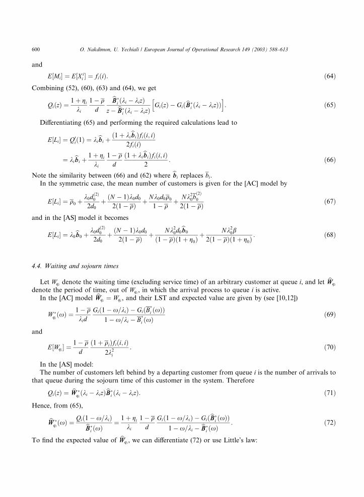
E½Mi� ¼ E½X ii � ¼ fiðiÞ: ð64ÞCombining (52), (60), (63) and (64), we get

QiðzÞ ¼1þ gi

ki

1� qd



GiðzÞh

� GiðbBB�i ðki � kizÞÞ

i: ð65Þ

Differentiating (65) and performing the required calculations lead to

E½Li� ¼ Q0ið1Þ ¼ kibbbi þ ð1þ kibbbiÞfiði; iÞ

2fiðiÞ

¼ kibbbi þ 1þ giki

1� qd

ð1þ kibbbiÞfiði; iÞ2

: ð66Þ

Note the similarity between (66) and (62) where bbbi replaces bi.In the symmetric case, the mean number of customers is given for the [AC] model by

E½Li� ¼ q0 þk0d

ð2Þ0

2d0þ ðN � 1Þk0d0

2ð1� qÞ þ Nk0d0q0

1� qþ Nk2

0bð2Þ0

2ð1� qÞ ð67Þ

and in the [AS] model it becomes

E½Li� ¼ k0bbb0 þ k0d

ð2Þ0


2ð1� qÞ þ Nk20d0bbb0

ð1� qÞð1þ g0Þþ Nk2

0b2ð1� qÞð1þ g0Þ

: ð68Þ

4.4. Waiting and sojourn times

Let Wqi denote the waiting time (excluding service time) of an arbitrary customer at queue i, and let bWWqi

denote the period of time, out of Wqi , in which the arrival process to queue i is active.

In the [AC] model bWWqi ¼ Wqi , and their LST and expected value are given by (see [10,12])

W �qiðxÞ ¼ 1� q

kidGið1� x=kiÞ � GiðB

�i ðxÞÞ

1� x=ki � B�i ðxÞ

ð69Þ

and

E½Wqi � ¼1� qd

ð1þ qiÞfiði; iÞ2k2

i

: ð70Þ

In the [AS] model:

The number of customers left behind by a departing customer from queue i is the number of arrivals to

that queue during the sojourn time of this customer in the system. Therefore

QiðzÞ ¼ bWW �qiðki � kizÞbBB�

i ðki � kizÞ: ð71Þ

Hence, from (65),

bWW �qiðxÞ ¼ Qið1� x=kiÞbBB�

i ðxÞ¼ 1þ gi

ki

1� qd

Gið1� x=kiÞ � GiðbBB�i ðxÞÞ

1� x=ki � bBB�i ðxÞ

: ð72Þ

To find the expected value of bWWqi , we can differentiate (72) or use Little’s law:


E½ bWWqi � ¼ � bWW �0qið0Þ ¼ E½Li�

ki� bbbi ¼ 1þ kibbbi

2ki

fiði; iÞfiðiÞ

: ð73Þ

Li is also the number of customers found in the queue by an arriving customer. This follows since the

system-state changes by unit jumps (see [7]). Then the waiting time of a customer in queue i is bWWqi with the

addition of the arrival stoppage periods that took place during the service periods of all the customers whowhere present in the system when he arrived:

Wqi ¼ bWWqi þXLij¼1

½BðjÞi � bBBðjÞ

i �: ð74Þ

Thus,

E½Wqi � ¼ E bWWqi

h iþ E½Li�E Bi

h� bBBii ¼ E½Li�

ki� bbbi þ E½Li�ðbi � bbbiÞ ¼ E½Li�

1þ giki

� bbbi: ð75Þ

Substituting E½Li� from (66) in (75) we get:

E½Wqi � ¼ kibbbi

þ 1þ giki

1� qd


!1þ gi

ki� bbbi

¼ 1þ giki

� �21� qd


þ gibbbi: ð76Þ

In the symmetric case, the mean waiting time is given for the [AC] model by

E½Wqi � ¼dð2Þ0

2d0þ ðN � 1Þd0

2ð1� qÞ þ Nd0q0

1� qþ Nk0b

ð2Þ0

2ð1� qÞ ð77Þ

and in the [AS] model, using (75) and (68), it becomes

E½Wqi � ¼ð1þ g0Þd

ð2Þ0

2d0þ ðN � 1Þð1þ g0Þd0

2ð1� qÞ þ Nk0d0bbb01� q

þ Nk0b2ð1� qÞ þ g0

bbb0: ð78Þ

Finally, the mean sojourn time of an arbitrary customer in queue i is given by

E½Wi � ¼ E½Wqi � þ bi ¼ E½Li�1þ gi

ki� bbbi þ bi ¼ E½Li�ð1þ giÞ þ gi

ki: ð79Þ

5. The Exhaustive regime

5.1. System-state: law of motion, PGFs and first moments

In the Exhaustive regime, in each visit, the server leaves a station only when it becomes empty.

Let Hi denote the length of a ‘busy period’ generated by a single customer in queue i. Let H�i ð�Þ, hi and

hð2Þi denote the LST of Hi, its mean and its second moment, respectively.

The evolution laws for the system-state are


PX iim¼1 HðmÞ

i


AiðDiÞ; j ¼ i;

(ð80Þ


where HðmÞi � Hi for every m, and they are mutually independent. Then (see [10,12])

Fiþ1ðzÞ ¼ Fi½z1; . . . ; zi�1;H�i ðriðzÞÞ; ziþ1; . . . ; zN �D�

i ðrðzÞÞ; ð81Þand by differentiating (81) or directly from (80),

fiþ1ðjÞ ¼fiðjÞ þ kjhifiðiÞ þ kjdi; j 6¼ i;kidi; j ¼ i:

�ð82Þ

In the [AC] model, Hi is a regular busy period of an M=G=1 type, but with service times Bi to customersin queue i. It is well known (see [7]) that

H�i ðxÞ ¼ B

�i ½x þ kið1� H�

i ðxÞÞ�; ð83Þ

hi ¼ E½Hi� ¼bi

1� qi; ð84Þ

hð2Þi ¼ E½H2

i � ¼bð2Þi

ð1� qiÞ3: ð85Þ

Therefore, the corresponding polling model may be viewed as a ‘standard’ one for which (see [10,12])

fiðjÞ ¼kj d

1�q

Pi�1

k¼jþ1 qk þPi�1

k¼j dkh i

; j 6¼ i;

kið1� qiÞ d1�q ; j ¼ i:

(ð86Þ

In the [AS] model:

Hi ¼ Bi þXAiðB̂BiÞm¼1

HðmÞi : ð87Þ

Hence,

H�i ðxÞ ¼ E

X1n¼0

P ½AiðbBBiÞ(

¼ njbBBi�E½e�xHi jBi; bBBi;AiðbBBiÞ ¼ n�)

¼ EX1n¼0

e�kibBBi ðkibBBiÞnn!

e�xBiE exp

"(� x

Xnm¼1

HðmÞi

!#)¼ E e�kibBBi�xBi

X1n¼0

ðkibBBiH�i ðxÞÞn

n!

( )

¼ E expð"

� xBi � kið1� H�i ðxÞÞbBBiÞ

#:

ð88ÞUsing (13), the definition of bBBi, and by conditioning on Ki we get

H�i ðxÞ ¼

X1k¼0

ð1� aiÞkaiE exp

"� x Sþi

"þXkm¼1

S�ðmÞi

�þ V ðmÞ

i

�#� kið1� H�

i ðxÞÞ Sþi

"þXkm¼1

S�ðmÞi

#!#

¼ aiSþ�

i ½x þ kið1� H�i ðxÞÞ�

X1k¼0

ð1� aiÞkfS��

i ½x þ kið1� H�i ðxÞÞ�gk½V �

i ðxÞ�k

¼ aiSþ�

i ½x þ kið1� H�i ðxÞÞ�

1� ð1� aiÞS��i ½x þ kið1� h�

i ðxÞÞ�V �i ðxÞ :

ð89ÞThe first and second moments of the busy period in the [AS] model can be calculated by differentiating (89),or directly from (87), as follows:


hi ¼ bi þ kibbbihi; implying

hi ¼bi

1� kibbbi :ð90Þ

hð2Þi ¼ E½H2

i � ¼ bð2Þi þ 2kiE½BibBBi�hi þ kibbbihð2Þ

i þ E AiðbBBiÞ AiðbBBiÞ�h� 1�i

h2i : ð91Þ

Using (90) and the definition of qi, we get:

kihi ¼kibi

1� kibbbi ¼ kibi1þ gi

,1� kibbbi1þ gi

!¼ qi

,1þ gi � kibi

1þ gi

� �¼ qi

1� qi: ð92Þ

Now,

E AiðbBBiÞ AiðbBBiÞ�h� 1�i

¼ EbBBi X1k¼0

kðk"

� 1Þe�kibBBi ðkibBBiÞkk!

#¼ EbBBi ðkibBBiÞ2e�kibBBiX1

k¼2

ðkibBBiÞk�2

ðk � 2Þ!

" #¼ k2

ibbbð2Þi : ð93Þ

By combining (91)–(93), we get:

hð2Þi ¼ b

ð2Þi þ 2qi

1� qiE½BibBBi� þ kibbbihð2Þ

i þ qi1� qi

� �2bbbð2Þi ;

leading to

hð2Þi ¼ ð1� qiÞ

2bð2Þi þ 2qið1� qiÞE½BibBBi� þ q2

ibbbð2Þi

ð1� kibbbiÞð1� qiÞ2

¼ ð1� qiÞ2b

ð2Þi þ 2qið1� qiÞE½BibBBi� þ q2

ibbbð2Þi

ð1þ giÞð1� qiÞ3

ð94Þ

(note, while comparing to (85), that the numerator of (94) is a convex combination of bð2Þi , bbbð2Þi and E½BibBBi�).

Summing (82) over all i givesXNi¼1

fiþ1ðjÞ ¼XNi¼1i6¼j

fiðjÞ þ kjXNi¼1i 6¼j

hifiðiÞ þ kjd ) fjðjÞ ¼ kjXNi¼1

hifiðiÞ � kjhjfjðjÞ þ kjd:

Thus,

fjðjÞ ¼kj

1þ kjhjd

þXNi¼1

hifiðiÞ!: ð95Þ

Multiplying (95) by hj and summing over all j yieldXNj¼1

hjfjðjÞ ¼ d

þXNi¼1

hifiðiÞ!XN

j¼1

kjhj1þ kjhj

: ð96Þ

Using (92) for the expression of kjhj, we get

kjhj1þ kjhj

¼qj

1� qj

21

1� qj¼ qj: ð97Þ

Substituting (97) in (96) leads to


XNj¼1

hjfjðjÞ ¼ d

þXNi¼1

hifiðiÞ!

q

from whichXNi¼1

hifiðiÞ ¼dq

1� q: ð98Þ

Now, using (92) again,

kj1þ kjhj

¼ kj

21

1� qj¼ kjð1� qjÞ: ð99Þ

Substituting results (98) and (99) in (95) we get

fjðjÞ ¼ kjð1� qjÞ d�

þ dq1� q

�¼ kjð1� qjÞ

d1� q

: ð100Þ

Using (82) and by proper summation we have

fiðjÞ ¼ kjXi�1

k¼jþ1

hkfkðkÞ"

þXi�1

k¼jdk

#: ð101Þ

Combining (92) with (100) leads to:

hkfkðkÞ ¼ qkd

1� qð102Þ

and therefore, using (101),

fiðjÞ ¼ kjd

1� q

Xi�1

k¼jþ1

qk

"þXi�1

k¼jdk

#: ð103Þ

Note that expressions (100) and (103) for the first-order moments in the [AS] model now look the ‘same’

as in the [AC] model (see Eq. (86)). However, the values of the fqig in each model are different.

5.2. Second-order moments

In both [AC] model and [AS] model, Eqs. (54) have the same expressions (of course, hi and hð2Þi have

different values in each model). After lengthy calculations we derive:


ð2Þi

fiþ1ði; jÞ ¼ kikjdð2Þi þ kidi½fiðjÞ þ kjhifiðiÞ�

oj 6¼ i

fiþ1ðj; kÞ ¼ kjkkdð2Þi þ kikkfiðiÞ½2dihi þ hð2Þ

i � þ kjkkh2i fiði; iÞ

þkjdifiðkÞ þ kkdifiðjÞ þ kkhifiði; jÞ þ kjhifiði; kÞþfiðj; kÞ

9=; j 6¼ ik 6¼ i

9>>>>>=>>>>>;: ð104Þ

In the symmetric case, in both [AC] model and [AS] model, using similar definitions as for the Gated re-

gime, we obtain:

fiði; iÞ ¼Nk2

0ð1� q0Þð1� qÞ dð2Þ0

(þ ðN � 1Þd20

1� qþ ðN � 1Þk0d0ð1� q0Þ

2

1� qhð2Þ0

); ð105Þ

where we set hi ¼ h0 and hð2Þi ¼ hð2Þ

0 , for i ¼ 1; 2; . . . ;N .


5.3. PGF and mean of number of customers

We use (60) again to find the PGF of Li and its expected value. In the [AC] model, the expressions are

given by (see [10,12])

QiðzÞ ¼1� qkid

B�i ðki � kizÞ

z� B�i ðki � kizÞ

½GiðzÞ � 1�; ð106Þ

E½Li� ¼ qi þk2i b

ð2Þi

2ð1� qiÞþ 1� q

dfiði; iÞ

2kið1� qiÞ¼ qi þ

k2i b

ð2Þi

2ð1� qiÞþ fiði; iÞ

2fiðiÞ: ð107Þ

The [AS] model requires additional calculations: Let bHHi denote the period of time, out of Hi, in which

customers arrive to queue i, and let bHH�i ð�Þ and bhhi denote its LST and its expected value, respectively. Then,

as in (83) and (84),bHH�i ðxÞ ¼ bBB�

i ½x þ kið1� bHH�i ðxÞÞ� ð108Þ

and

bhhi ¼ E½ bHHi� ¼bbbi

1� kibbbi : ð109Þ

Now, using (100) and (109),

E½Mi� ¼ fiðiÞ½1þ kibhhi� ¼ kið1� qiÞd

1� q1

"þ kibbbi1� kibbbi

#¼ ki

1� kibbbi1þ gi

d1� q

1

1� kibbbi¼ ki

1þ gi

d1� q

; ð110Þ

EXMin¼1

zLiðnÞ" #

¼ PiðzÞz� PiðzÞ

½GiðzÞ � 1� ðsee ½10�Þ; ð111Þ

where PiðzÞ is the PGF of the number of customers arrived to queue i during a (generalized) service time of a

single customer. Then, for the [AS] model,

PiðzÞ ¼ bBB�i ðkið1� zÞÞ: ð112Þ

Combining (60), (110), (111) and (112) gives the PGF of Li:

QiðzÞ ¼1þ gi

ki

1� qd



½GiðzÞ � 1�: ð113Þ

Differentiating (113) and performing some calculations lead to

E½Li� ¼ Q0ið1Þ ¼ kibbbi þ k2

ibbbð2Þi

2ð1� kibbbiÞ þ fiði; iÞ2fiðiÞ¼ kibbbi þ k2

ibbbð2Þi

2ð1� kibbbiÞ þ 1� qd

fiði; iÞ2kið1� qiÞ

: ð114Þ

In the symmetric case, the mean number of customers is given for the [AC] model by (see [10])


E½Li� ¼ q0 þk0d

ð2Þ0


2ð1� qÞ þ Nk20b

ð2Þ0

2ð1� qÞ ð115Þ

and in the [AS] model it becomes

E½Li� ¼ k0bbb0 þ k0d

ð2Þ0


2ð1� qÞ þ Nk20b

2ð1� qÞð1þ g0Þ: ð116Þ

5.4. Waiting and sojourn times

In the [AC] model the LST and the expected value of the waiting times are given by (see [10,12]):

W �qiðxÞ ¼ 1� q

kidGið1� x=kiÞ � 1

1� x=ki � B�i ðxÞ

; ð117Þ

E½Wqi � ¼kib

ð2Þi

2ð1� qiÞþ 1� q

dfiði; iÞ

2k2i ð1� qiÞ

: ð118Þ

In [AS] model, define bWWqi (as in the Gated regime) to be the period of time out of Wqi , in which the arrival

process to queue i is active.

Then, using the general relation (71) and (113),

bWW �qiðxÞ ¼ Qið1� x=kiÞbBB�

i ðxÞ¼ 1þ gi

ki

1� qd

Gið1� x=kiÞ � 1

1� x=ki � bBB�i ðxÞ

: ð119Þ

To find the expected value of bWWqi , we can differentiate (119) or use Little’s law:

E½ bWWqi � ¼ � bWW �0qið0Þ ¼ E½Li�

ki� bbbi ¼ kibbbð2Þi

2ð1� kibbbiÞ þ fiði; iÞ2kifiðiÞ

: ð120Þ

By substituting E½Li� from (114) in (75), we finally obtain:

E½Wqi � ¼ kibbbi

þ k2ibbbð2Þi

2ð1� kibbbiÞ þ fiði; iÞ2fiðiÞ

!1þ gi

ki� bbbi

¼ k2ibbbð2Þi

2ð1� kibbbiÞ

þ 1� qd

fiði; iÞ2kið1� qiÞ

!1þ gi

kiþ gibbbi: ð121Þ

In the symmetric case, the mean waiting time is given for the [AC] model by (see [5,10])

E½Wqi � ¼dð2Þ0

2d0þ ðN � 1Þd0

2ð1� qÞ þ Nk0bð2Þ0

2ð1� qÞ ; ð122Þ

and in the [AS] model, using (75) and (116), it becomes:

E½Wqi � ¼ð1þ g0Þd

ð2Þ0

2d0þ ðN � 1Þð1þ g0Þd0

2ð1� qÞ þ Nk0b2ð1� qÞ þ g0

bbb0: ð123Þ

The above results have the following important consequence:

It follows from (77) and (122), as well as from (78) and (123), that for the symmetric cases in both models


E½WqiðGatedÞ� ¼ E½WqiðExhaustiveÞ� þNk0d0bbb01� q

ð124Þ

(remember that in the [AC] model q0 ¼ k0b0 ¼ k0bbb0Þ. That is, for both models, as in the regular symmetric

polling schemes

E½WqiðExhaustiveÞ� < E½WqiðGatedÞ�: ð125Þ

6. Common results

Combining the above results, it follows that for both regimes (Gated and Exhaustive), for both models

([AC] and [AS]) and for both versions (breakdown observation upon occurrence or at end of service), we can

derive a common (generalized) expression for fiðiÞ, the mean number of customers in a queue at a polling

instant of that queue (see Eq. (126) below). As a result of that, we obtain some generalized expressions for

other important parameters. With bi having the corresponding values for each version, and with hi ex-pressing the mean busy period generated by a customer (which for the Gated regime equals the meanservice time of a single customer) we construct the following table:

It follows that in all cases, for i ¼ 1; 2; . . . ;N ,

fiðiÞ ¼qihi

d1� q

: ð126Þ

By using (126) the mean cycle time (for all models, all versions and all regimes) is given by a common

expression:

E½C� ¼ d þXNi¼1

fiðiÞhi ¼ d þ d1� q

XNi¼1

qihi

hi ¼ d þ d1� q

q ¼ d1� q

: ð127Þ

It follows from (127) that a necessary condition for stability is q < 1. Now, from (126),

fiðiÞ ¼qihiE½C�; ð128Þ

and therefore, the mean sojourn time of the server at queue i is

fiðiÞhi ¼ qiE½C�: ð129Þ

Regime Model qi hi fiðiÞGated AC kibi bi ki

d1� q

ASkibi1þ gi

biki

1þ gi

d1� q

Exhaustive AC kibibi

1� qikið1� qiÞ

d1� q

ASkibi1þ gi

bi1� kibbbi kið1� qiÞ

d1� q


Thus, qi is the fraction of time the server resides in queue i. We use this result to calculate the mean arrival

rate to queue i, Ki, which is composed of weighted effective arrival rates, with weights qi and ð1� qiÞ,respectively:

Ki ¼ qibbbibi

ki

"þ 1

�bbbibi

!0

#þ ð1� qiÞki ¼ ki 1

"� qi 1

�bbbibi

!#¼ ki 1

"� kibi1þ gi

bi � bbbibi

#

¼ ki 1

�� gi1þ gi

�¼ ki

1þ gi¼ qibi: ð130Þ

Accordingly, the work rate (traffic load) of queue i is

Kibi ¼ qi ð131Þ

and the total traffic load of the system is indeed the generalized q (see remark after Eq. (50)). It follows (see

[4]) that q < 1 is not only a necessary condition for stability, but also a sufficient one. From (129), the mean

number of customers served in queue i during a cycle is

E½Mi� ¼qiE½C�bi

¼ ki1þ gi

E½C�; ð132Þ

which coincides with the results obtained separately for each of the regimes (Eqs. (52) and (64) for the

Gated, and Eq. (110) for the Exhaustive).

7. The Globally Gated regime

In the (cyclic) Globally Gated (GG) regime [1,2], as in the Gated and Exhaustive regimes, the server

visits the queues in a cyclic order. However, at the initiation of every new cycle all gates are simultaneously

closed, so that only those customers present in the system at that instant are served during that cycle.

We assume, without loss of generality, that a cycle starts from queue 1.Let Xj X j1 ¼ the number of customers at queue j at a cycle-beginning. Let fj EðXjÞ f1ðjÞ.In the [AC] model (see [12]):

C�ðxÞ ¼ D�ðxÞC�XNj¼1

kj 1�"

� B�j ðxÞ

�#; ð133Þ

E½C� ¼ d1� q

; ð134Þ

E½C2� ¼ 1

1� q2dð2Þ"

þ 2dq

þXNj¼1

kjbð2Þj

!E½C�

#; ð135Þ

where D PN

j¼1 Dj and dð2Þ is its second-order moment.

In both models, the number of customers present at queue j at a cycle-beginning is the number of

customers that arrived at queue j during a (previous) cycle. However, in the [AS] model, the arrival process

to queue j stops during repair times at that queue, and therefore, in steady state,

Xj ¼ Aj C

�XXjk¼1

ðBðkÞj � bBBðkÞ

j Þ!; ð136Þ


where BðkÞj � Bj and bBBðkÞ

j � bBBj for every k. It follows thatfj ¼ kjðE½C� � fjðbj � bbbjÞÞ ¼ kjE½C� � fjgj; leading to

fj ¼kjE½C�1þ gj

:ð137Þ

Now,

C ¼ DþXNj¼1

XXjk¼1

BðkÞj : ð138Þ

Hence, with F1ðzÞ EQNj¼1 z

Xjj

h i, we get

C�ðxÞ ¼ D�ðxÞF1 B�i ðxÞ;B�

2ðxÞ; . . . ;B�N ðxÞ

� �ð139Þ

and

E½C� ¼ d þXNj¼1

fjbj: ð140Þ

Substituting fj from (137), we have

E½C� ¼ d þXNj¼1

kjbj1þ gj

E½C� ¼ d þ qE½C�;

leading to, as in the other regimes,

E½C� ¼ d1� q

: ð141Þ

Thus,

fj ¼kj

1þ gj

d1� q

: ð142Þ

That is, f1ðjÞGG ¼ fjðjÞGated.

7.1. Waiting times

To be able to obtain expressions for the mean waiting time of a customer in queue i in the two models we

need an expression for the second-order moment of a cycle. From (138) we get:

E½C2� ¼ E D2

8<: þ 2DXNj¼1

XXjk¼1

BðkÞj þ

XNj¼1

XXjk¼1

BðkÞj

!29=;: ð143Þ

After some algebraic manipulations (see Appendix A) we obtain:

E½C2� ¼dð2Þ þ 2dq þ

PNj¼1

kjbð2Þj

1þgjþ kjq

2j

1�gjðbð2Þj � 2E½BjbBBj� þ bbbð2Þj Þ

� �� E½C�

1� q2: ð144Þ

Now, for both models, let CP CR denote, respectively, the past and residual duration of a cycle. Then (see [1]):

C�PðxÞ ¼ C�

RðxÞ ¼ 1� C�ðxÞxE½C� ð145Þ


and

E½CP� ¼ E½CR� ¼E½C2�2E½C� : ð146Þ

Consider an arbitrary customer J at queue j. His waiting time is composed of

(i)iva residual cycle time CR,

(ii)vthe service times of all customers who arrive at queues 1; 2; . . . ; j� 1 during the cycle in which J arrives,

(iii) the switchover times of the server between queues 1; 2; . . . ; j� 1 and j, and(iv) the service times of all customers who arrived at queue j before J, i.e. during the past part CP of the

cycle in which J arrives.

Then,

E½Wqj � ¼ E½CR� þXj�1

k¼1

E½AkðCP þ CRÞ�bk þXj�1

k¼1

dk þ E½AjðCPÞ�bj: ð147Þ

In the [AC] model Eq. (147) becomes (see [1])

E½Wqj � ¼ 1

þ 2

Xj�1

k¼1

qk þ qj

!E½CR� þ

Xj�1

k¼1

dk: ð148Þ

In the [AS] model the calculation of E½AkðCPÞ� is much more complicated. In order to find E½AkðCPÞ� weconsider the three possible cases for the position of the server at the instant of arrival of customer J.

(1) the server is before queue k;

(2) the server is in queue k; and

(3) the server has passed queue k.

The probabilities for these cases are, respectively, sk=E½C�, qk and 1� qk � ðsk=E½C�Þð Þ, where sk is

the mean time from the start of a cycle until the server enters queue k. From (129), sk ¼Pk�1

m¼1 ðqmE½C� þ dmÞ. The arrival rate to queue k when the server is in that queue is kkðbbbk=bkÞ, and it equals

kk when the server is not in queue k. Therefore, an approximation to E½AkðCPÞ�, based on an assumption of

independence between the various elements, is given by

E½AkðCPÞ� ¼skE½C� kkE½CP� þ qk kksk

"þ kk

bbbkbk

ðE½CP� � skÞ#þ 1

�� qk �

skE½C�

�kkbbbkbk

qkE½C�"

þ kkðE½CP� � qkE½C�Þ#

¼ kk qkbbbkbk

(þ 1� qk

!E½CP� þ qk 1

�bbbkbk

!½2sk � E½C�ð1� qkÞ�

)

¼ kk E½CP��

� gk1þ gk

E½CP� þgk

1þ gk½2sk � E½C�ð1� qkÞ�

0¼ kk

1þ gk½EðCPÞ þ 2gksk � gkð1� qkÞEðCÞ�: ð149Þ


In a similar way,

E½AkðCRÞ� ¼skE½C� kk

bbbkbk

qkE½C�"

þ kkðE½CR� � qkE½C�Þ#þ qk kk½ð1

"� qkÞE½C� � sk�

þ kkbbbkbk

½E½CR� � ð1� qkÞE½C� þ sk�#þ 1

�� qk �

skE½C�

�kkE½CR�

¼ kk qkbbbkbk

(þ 1� qk

!E½CR� � qk 1

�bbbkbk

!½2sk � E½C�ð1� qkÞ�

)

¼ kk E½CR��

� gk1þ gk

E½CR� �gk

1þ gk2sk½ � E½C�ð1� qkÞ�

0

¼ kk1þ gk

½EðCRÞ � 2gksk þ gkð1� qkÞEðCÞ�: ð150Þ

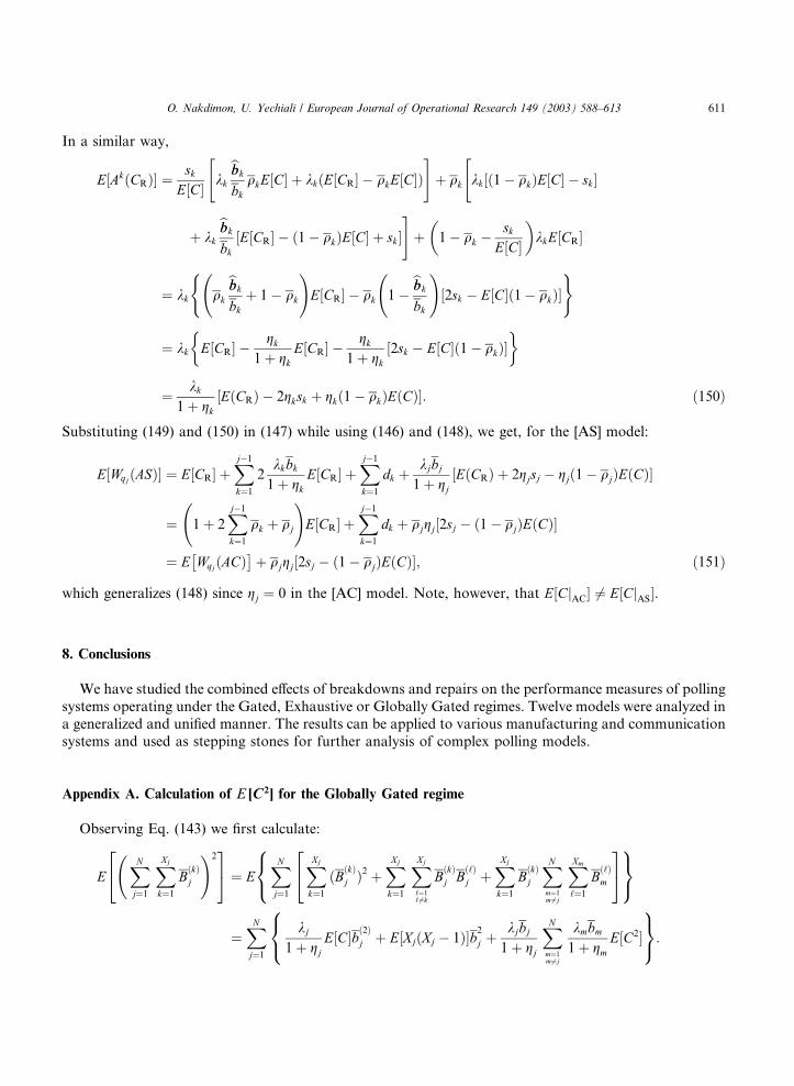
Substituting (149) and (150) in (147) while using (146) and (148), we get, for the [AS] model:

E½WqjðASÞ� ¼ E½CR� þXj�1

k¼1

2kkbk1þ gk

E½CR� þXj�1

k¼1

dk þkjbj1þ gj

½EðCRÞ þ 2gjsj � gjð1� qjÞEðCÞ�

¼ 1

þ 2

Xj�1

k¼1

qk þ qj

!E½CR� þ

Xj�1

k¼1

dk þ qjgj½2sj � ð1� qjÞEðCÞ�

¼ E WqjðACÞ� �

þ qjgj½2sj � ð1� qjÞEðCÞ�; ð151Þ

which generalizes (148) since gj ¼ 0 in the [AC] model. Note, however, that E½CjAC� 6¼ E½CjAS�.

8. Conclusions

We have studied the combined effects of breakdowns and repairs on the performance measures of polling

systems operating under the Gated, Exhaustive or Globally Gated regimes. Twelve models were analyzed ina generalized and unified manner. The results can be applied to various manufacturing and communication

systems and used as stepping stones for further analysis of complex polling models.

Appendix A. Calculation of E [C2] for the Globally Gated regime

Observing Eq. (143) we first calculate:

EXNj¼1

XXjk¼1

BðkÞj

!224 35 ¼ E

XNj¼1

XXjk¼1

ðBðkÞj Þ2

248<: þXXjk¼1

XXj‘¼1‘ 6¼k

BðkÞj B

ð‘Þj þ

XXjk¼1

BðkÞj

XNm¼1m6¼j

XXm‘¼1

Bð‘Þm

359=;¼XNj¼1

kj1þ gj

E½C�bð2Þj

8<: þ E½XjðXj � 1Þ�b2j þkjbj1þ gj

XNm¼1m6¼j

kmbm1þ gm

E½C2�

9=;:


Similarly to the derivation of Eq. (93), we get,

E½XjðXj � 1Þ� ¼ k2j E C

24 �XXjk¼1


j Þ!235

¼ k2j E C2

"� 2C

XXjk¼1


j Þ þXXjk¼1


j Þ2#

þ k2j E

XXjk¼1

XXjm¼1m 6¼k

ðBðkÞj

24 � bBBðkÞj ÞðBðmÞ

j � bBBðmÞj Þ

35¼ k2

j E½C2�"

� 2kj

1þ gjðbj � bbbjÞE½C2� þ kj

1þ gjE½C�½bð2Þj � 2E½BjbBBj� þ bbbð2Þj �

#þ k2

j E½XjðXjh

� 1Þ�ðbj � bbbjÞ2i) E½XjðXj � 1Þ� ¼

k2j

1� g2j

1� gj1þ gj

E½C2�(

þ kj1þ gj

E½C�½bð2Þj � 2E½BjbBBj� þ bbbð2Þj �)

) E½XjðXj � 1Þ�b2j ¼ q2j E½C2� þ kj

1� gjq2j E½C� b

ð2Þj

h� 2E½BjbBBj� þ bbbð2Þj i

) EXNj¼1

XXjk¼1

BðkÞj

!224 35

¼XNj¼1

kjbð2Þj

1þ gjE½C�

(þ q2

j E½C2� þkjq2

j

1� gjbð2Þj

�� 2E½BjbBBj� þ bbbð2Þj �E½C�

)

þ q2

�XNj¼1

q2j

!E½C2�: ðA:1Þ

By substituting (A.1) in (143) we get

E½C2� ¼ dð2Þ þ 2dpE½C� þXNj¼1

kjbð2Þj

1þ gj

(þ

kjq2j

1� gjðbð2Þj � 2E½BjbBBj� þ bbbð2Þj Þ

)E½C� þ q2E½C2�; ðA:2Þ

which leads to Eq. (144).

References

[1] O.J. Boxma, H. Levy, U. Yechiali, Cyclic reservation schemes for efficient operation of multiple-queue single-server systems,

Annals of Operations Research 35 (1992) 187–208.

[2] O.J. Boxma, J.A. Weststrate, U. Yechiali, A globally gated polling system with server interruptions and applications to the

repairman problem, Probability in the Engineering and Informational Sciences 7 (1993) 187–208.

[3] R.W. Conway, W.L. Maxwell, L.W. Miller, Theory of Scheduling, Addison-Wesley, Reading, MA, 1967.

[4] C. Fricker, M.R. Ja€ııbi, Monotonicity and stability of periodic polling models, Queueing Systems 15 (1994) 211–238.

[5] O. Hashida, Analysis of multiqueue, Review of the Electrical Communication Laboratories 20 (1972) 189–199.

[6] O. Hashida, Gating multiqueues served in cyclic order, Systems–Computers–Controls 1 (1970) 1–8.


[7] L. Kleinrock, Queueing Systems, vol. 1 Theory, John Wiley and Sons, New York, 1975.

[8] D. Kofman, U. Yechiali, Polling systems with station breakdowns, Performance Evaluation 27&28 (1996) 647–672.

[9] D. Kofman, U. Yechiali, Queueing networks with station breakdowns and globally gated regime, in: V. Ramaswamy, P.E. Wirth

(Eds.), Teletraffic Contributions for the Information Age, North Holland, Amsterdam, 1997, pp. 285–296.

[10] H. Takagi, Analysis of Polling Systems, MIT Press, Cambridge, MA, 1986.

[11] H. Takagi, Queueing analysis of polling models: An update, in: H. Takagi (Ed.), Stochastic Analysis of Computer and

Communication Systems, North Holland, Amsterdam, 1990, pp. 267–318.

[12] U. Yechiali, Analysis and control of polling systems, in: L. Donatiello, R. Nelson (Eds.), Performance Evaluation of Computer

and Communications Systems, Springer-Verlag, 1993, pp. 630–650.


polling systems with breakdowns and repairs

Documents