policy instruments to lean against the wind in latin america; by

Policy Instruments To Lean Against The Wind In Latin America

Gilbert Terrier, Rodrigo Valdés, Camilo E. Tovar, Jorge Chan-Lau, Carlos Fernández-Valdovinos, Mercedes García-

Escribano, Carlos Medeiros, Man-Keung Tang, Mercedes Vera Martin, and Chris Walker

WP/11/159

© 2011 International Monetary Fund WP/11/159

IMF Working Paper

Western Hemisphere Department

Policy Instruments To Lean Against The Wind In Latin America

Prepared by Gilbert Terrier, Rodrigo Valdés, Camilo E. Tovar, Jorge Chan-Lau, Carlos Fernández-Valdovinos, Mercedes García-Escribano, Carlos Medeiros, Man-Keung Tang

Mercedes Vera Martin, and Chris Walker

Authorized for distribution by Nicolás Eyzaguirre

July 2011

Abstract

This Working Paper should not be reported as representing the views of the IMF. The views expressed in this Working Paper are those of the author(s) and do not necessarily represent those of the IMF or IMF policy. Working Papers describe research in progress by the author(s) and are published to elicit comments and to further debate.

This paper reviews policy tools that have been used and/or are available for policy makers in the region to lean against the wind and review relevant country experiences using them. The instruments examined include: (i) capital requirements, dynamic provisioning, and leverage ratios; (ii) liquidity requirements; (iii) debt-to-income ratios; (iv) loan-to-value ratios; (v) reserve requirements on bank liabilities (deposits and nondeposits); (vi) instruments to manage and limit systemic foreign exchange risk; and, finally, (vii) reserve requirements or taxes on capital inflows. Although the instruments analyzed are mainly microprudential in nature, appropriately calibrated over the financial cycle they may serve for macroprudential purposes.

JEL Classification Numbers: E58, F32, F34, G28

Keywords: Capital Requirements, Dynamic Provisions, Leverage Ratios, Liquidity Requirements, Debt-to-Income Ratios, Loan-to-Value Ratios, Reserve Requirements, Foreign Exchange Credit Risk, Foreign Exchange Positions, Taxes on Capital Inflows

Author’s E-Mail Address: [email protected]; [email protected]; [email protected]; [email protected]; [email protected]; [email protected]; [email protected]; [email protected]; [email protected]; and [email protected], respectively.

Contents Page

Abstract ......................................................................................................................................2

I. Policy Instruments to Lean against the Wind in Latin America .............................................5 A. Overview ...................................................................................................................7

II. Capital Requirements, Leverage Ratios, Countercyclical Capital Buffers and Dynamic Provisions ............................................................................................................................10

A. Introduction .............................................................................................................10 B. The Tools and Their Objectives: Solvency and Leaning Against the Wind ...........10 C. Implications for Latin America ...............................................................................13 D. Conclusions .............................................................................................................21

III. Liquidity Requirements for Macroprudential Purposes .....................................................23 A. Motivation ...............................................................................................................23 B. The Liquidity Coverage Ratio (LCR) .....................................................................25 C. Net Stable Funding Ratio (NSFR) ..........................................................................26 D. Quantitative and Economic Impact of LCR and NSFR ..........................................27 E. Conclusions .............................................................................................................28

IV. Debt to Income limits ........................................................................................................38 A. Debt to Income Ratios .............................................................................................38 B. Risks Arising from Household Indebtedness ..........................................................39 C. Debt to Income Limits .............................................................................................40 D. Conclusion ..............................................................................................................42

V. Loan-to-Value Ratio Caps as a Macroprudential Tool .......................................................43 A. Introduction .............................................................................................................43 B. LTV Rule Implementation ......................................................................................43 C. Existing Evidence on Effectiveness ........................................................................45 D. Recent Examples in the Americas ..........................................................................45 E. Conclusion ...............................................................................................................48

VI. Reserve Requirements on Bank Liabilities as a Macroprudential Tool ............................54 A. Introduction .............................................................................................................54 B. Theoretical Considerations ......................................................................................56 C. Conclusions .............................................................................................................58

VII. Macroprudential Instruments to Manage Foreign-Exchange Credit Risk ........................71 A. Motivation ...............................................................................................................71 B. Instruments and Potential Benefits ..........................................................................72

VIII. Limiting Foreign Exchange Positions to Contain Systemic Risk ...................................80 A. Introduction .............................................................................................................80 B. Potential Macroprudential Benefits .........................................................................82 C. Conclusions .............................................................................................................84

4

IX. Reserve Requirements and Taxes on Capital Inflows .......................................................94 A. Introduction .............................................................................................................94 B. Theoretical Considerations ......................................................................................95 C. Conclusions .............................................................................................................97

Boxes II. 1. Accounting Treatment of Provisions and Capital ....................................................12

2. Dynamic Provisions in Spain and Latin America ....................................................19 VI. 1. Effect of Changes in RRs on Active Interest Rates .................................................57 XI. 1. Tax-equivalent of RRs .............................................................................................96 Annexes III. 1. Country experiences: New Zealand, Colombia, Chile, and Australia .....................30 V. 1. Case Study of Hong Kong SAR...............................................................................50

2. Recent Country Examples of LTV Restrictions ......................................................53 VI. 1. Country experiences with Deposit Reserve Requirements ......................................60

2. Country experiences with Reserve Requirements on (non-core) ............................67 VII. 1. Country Experiences in Managing FX Credit Risk .................................................74 VIII. 1. Country Experiences and Case Studies ....................................................................85

2. Carry Trade Using Futures Market ..........................................................................93 IX. 1. Country Experiences with Reserve Requirements on Capital Inflows ....................99

5

I. POLICY INSTRUMENTS TO LEAN AGAINST THE WIND IN LATIN AMERICA1

Emerging market economies (EMEs), including Latin America, currently face a juncture of easy external financing conditions that are conducive to credit exuberance, asset price bubbles, and excess demand booms, which increase the risk to a sudden reversal (IMF, 2011c). Appropriately managing the procyclicality of the financial system is thus a policy priority to avoid the emergence of financial excesses and vulnerabilities in the banking sector and, more generally, in other segments of the economy (Eyzaguirre et al, 2011; IMF, 2010a,b,c and 2011a,e).

However, the use of traditional macroeconomic policy instruments to confront such external environment may run into limits. For instance, monetary policy can be constrained as interest rate hikes to contain financial exuberance are likely to trigger more capital flows, which would stimulate financial and economic excesses. Foreign exchange intervention is likely to have only temporary effects and may, at the same time, impose large quasi-fiscal costs (IMF 2011c). 2 Traditional instruments may also be inefficient to confront particular financial risks that build up in a boom.

In this context, macroprudential (MaP) tools and regulations constitute a complement to traditional macroeconomic policies. MaP policies along with prudent monetary and fiscal policies and microprudential (MiP) policies help manage the financial cycle and reduce the probability of boom-bust cycles. They also help avoid the accumulation of vulnerabilities that expose the financial system to additional stress in the down part of the cycle, e.g., due to fire sales or other events related to the increased interconnectedness of the financial system (IMF, 2010a, 2010c; Eyzaguirre et al, 2011).3 In some instances, MaP instruments may also complement some of the effects of monetary policy.

Despite the broad agreement on adopting a MaP approach for managing systemic risk, policy design is evolving and its implementation remains challenging. Many issues are under discussion, including the definition of systemic risk, how to track it, the level of granularity, the balance between rules and discretion, institutional arrangements and mandates, coordination and cooperation in supervision at the national and international levels (see IMF, 2010c and 2011d). Furthermore, there is a need to understand better when to use these tools and how they work in practice. This entails understanding how to design and calibrate them and, more importantly, identify their costs, benefits, and effectiveness.

1 Prepared by Gilbert Terrier, Rodrigo Valdes, and Camilo E. Tovar. 2 By delaying exchange rate adjustment, foreign exchange intervention may itself trigger more capital flows if it creates expectations of exchange rate appreciation. This highlights the challenges faced by traditional macroeconomic instruments, which may be themselves a source of heightened risk. 3 The distinction between MaP and microprudential (MiP) policies is best drawn in terms of objectives. MiP policy aims to reduce the probability of default of individual institutions, taking systemic risk as given; while MaP policy aims at preventing the economic and social costs of systemic financial distress, taking into account feedback effects that the behavior of individual institutions have on each other, and on the whole economy.

6

Nonetheless, many EMEs, including those of Latin America, have already employed different tools with MaP purposes, particularly to dampen the cycle and the associated risk taking. The authorities are actively engaged in deciding which tools to rely upon.

The notes in this volume review policy tools that have been used and/or are readily available for policy makers in Latin America. Each note describes how a specific instrument can serve MaP purposes, and reviews relevant country experiences―from the region or elsewhere (up to March 2011). Although not fully comprehensive, cross- country experience illustrates actual practices and, in some instances, serves as a gauge of their possible effects based on such experiences. Furthermore, some of the instruments are MiP in nature (see footnote 1), and may serve as an useful tool to achieve MaP goals when appropriately calibrated over the financial cycle. Specifically, the set of instruments examined include: (i) capital requirements, dynamic provisioning and leverage ratios; (ii) liquidity requirements; (iii) debt-to-income ratios; (iv) loan-to-value ratios; (v) reserve requirements on bank liabilities (deposits and nondeposits); (vi) instruments to manage and limit systemic foreign exchange risk; and, finally, (vii) reserve requirements or taxes on capital inflows.

This volume aims at being a timely compilation of practices on the use of instruments that could help lean against the wind. The notes are descriptive in nature, and are not aiming at establishing a policy guide on the use of such instruments. This explains the bottom-up approach of describing and examining individual instruments and country experiences, rather than a top-down approach that would require a careful analysis of how MaP policies interact with traditional policies, such as monetary and/or fiscal policy. The IMF is currently engaged in building up a consistent framework to analyze these issues (see IMF 2011a,d). Furthermore, the set of policies examined here need to be examined within a broader menu of policy options, including establishing the appropriate priorities and taking into account country’s specific conditions. Some of these broader issues have recently been examined in other IMF documents (Eyzaguirre et al, 2011; IMF 2011e; and Ostry and others, 2011 and 2010).

It is worth clarifying that systemic risk has been defined as the risk of disruption to financial services that is caused by an impairment of all or parts of the financial system and has the potential to have negative consequences on the real economy (IMF, 2010c and 2011d). It has two dimensions: (i) a cross-sectional dimension; and (ii) a time dimension. The first takes into account the distribution of risk across the financial and economic system, thus reflecting externalities across the system (e.g., common exposures, interconnectedness, or contagion). The second considers how system-wide risk evolves and is accumulated over time, taking into account the pro-cyclicality of the financial system.

From a Latin American perspective, addressing procyclicality is currently the main priority, given the pressures associated by large capital inflows. Latin American economies have not been negatively affected by the global financial crisis in a significant

7

way; they have recovered very quickly; and are already evidencing overheating pressures due, in part, to strong domestic demand dynamics in an environment of easy global financial conditions. This combination of factors is already leading to substantial credit growth in some countries, high asset prices, and raising concerns about the need to avoid financial excesses (See IMF, 2011c). Nonetheless, it is also important to pay attention to the lessons derived from the financial crisis in assessing and managing common exposures and interconnectedness in the financial system, especially because the presence of foreign banks in the region is significant. In this respect, more work will have to be done in monitoring and managing the risks emerging from systemically important financial institutions (SIFIs)including “too-big-to-fail” institutionsand in extending the perimeter of regulation to avoid the parallel development of a shadow financial system.

Overview

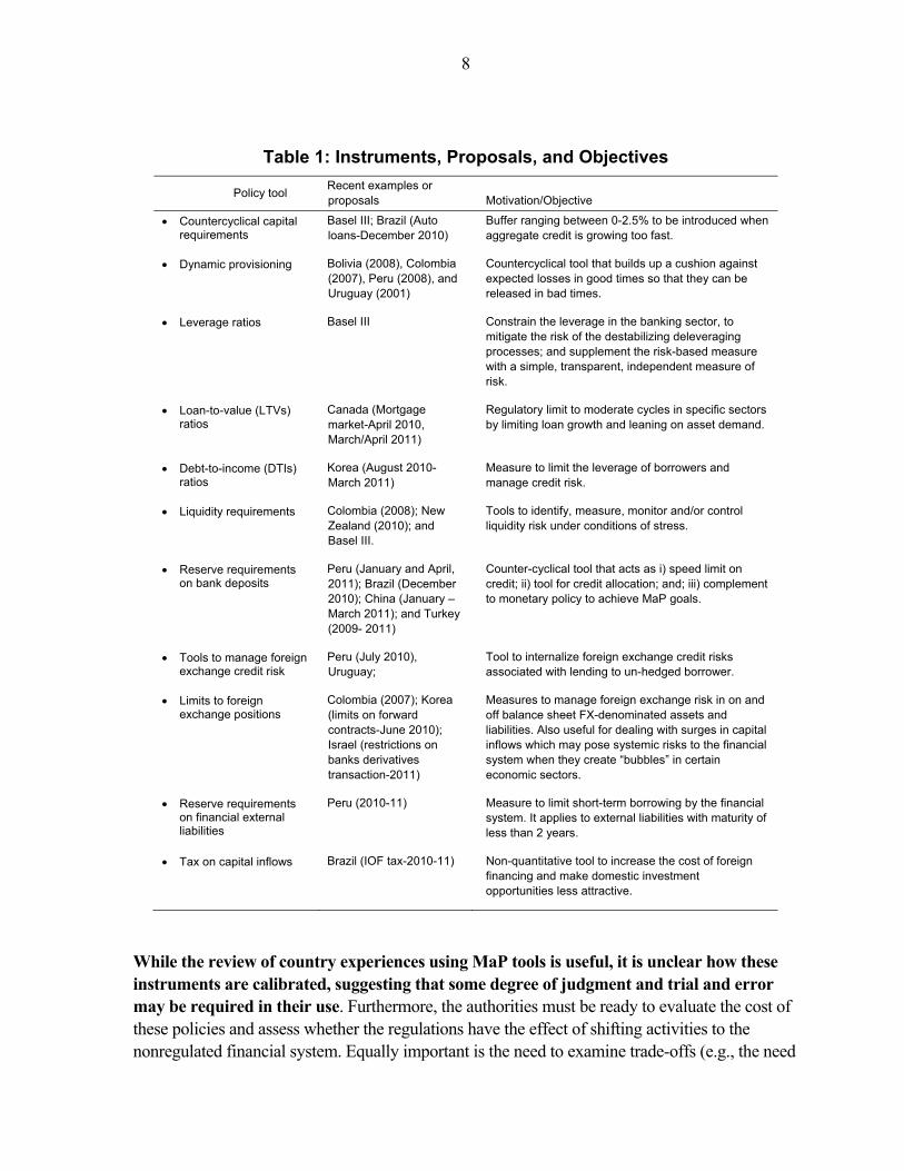
The analysis in this volume discusses how these instruments can help contain the accumulation of vulnerabilities that could arise in a context of easy global and domestic financial conditions (Table 1).4 In the upswing, the instruments examined can constrain or act as a speed limit on credit growth―both across the system or in specific sectors of the economyavoid excessive leverage of banks and debtors; and tilt the financing structure of the financial system toward more stable and longer-term sources. In other instances, they increase the cost of foreign financing for banks and make domestic investment opportunities less attractive to foreign investors. Moreover, they help manage credit, liquidity, solvency, and/or foreign exchange credit risks. These features reduce the vulnerability of the financial system to reversals in capital flows. In some instances, the instruments examined also aim at building buffers in good times which can be deployed in bad times. More generally, by helping manage the credit and asset price cycles, they can be an effective complement to monetary policy, even in inflation targeting regimes.

Given that there is no single MaP instrument able to address all aspects of systemic risk, a combination of different tools, tailored to country-specific needs, is required. For instance, some tools address specific risks (e.g., liquidity or credit), or sometimes are targeted at specific sectors (e.g., housing or foreign exchange market). Although most tools focus on regulating the banking system, risks are also likely to shift to the nonregulated financial system, signaling the need for an encompassing macro-financial management approach. Furthermore, evidence regarding the effectiveness of these tools needs to be refined and explored further, in part because these measures are not taken in isolation. A common issue across instruments is the lack of adequate theoretical frameworks to evaluate their effectiveness, in particular in a general equilibrium setting.

4 This table only summarizes recent changes in policies. It does not take stock of existing policies that may already be in place and be already tight.

8

Table 1: Instruments, Proposals, and Objectives

Policy tool Recent examples or proposals Motivation/Objective

Countercyclical capital requirements

Basel III; Brazil (Auto loans-December 2010)

Buffer ranging between 0-2.5% to be introduced when aggregate credit is growing too fast.

Dynamic provisioning Bolivia (2008), Colombia (2007), Peru (2008), and Uruguay (2001)

Countercyclical tool that builds up a cushion against expected losses in good times so that they can be released in bad times.

Leverage ratios Basel III Constrain the leverage in the banking sector, to mitigate the risk of the destabilizing deleveraging processes; and supplement the risk-based measure with a simple, transparent, independent measure of risk.

Loan-to-value (LTVs) ratios

Canada (Mortgage market-April 2010, March/April 2011)

Regulatory limit to moderate cycles in specific sectors by limiting loan growth and leaning on asset demand.

Debt-to-income (DTIs) ratios

Korea (August 2010-March 2011)

Measure to limit the leverage of borrowers and manage credit risk.

Liquidity requirements Colombia (2008); New Zealand (2010); and Basel III.

Tools to identify, measure, monitor and/or control liquidity risk under conditions of stress.

Reserve requirements on bank deposits

Peru (January and April, 2011); Brazil (December 2010); China (January –March 2011); and Turkey (2009- 2011)

Counter-cyclical tool that acts as i) speed limit on credit; ii) tool for credit allocation; and; iii) complement to monetary policy to achieve MaP goals.

Tools to manage foreign exchange credit risk

Peru (July 2010), Uruguay;

Tool to internalize foreign exchange credit risks associated with lending to un-hedged borrower.

Limits to foreign exchange positions

Colombia (2007); Korea (limits on forward contracts-June 2010); Israel (restrictions on banks derivatives transaction-2011)

Measures to manage foreign exchange risk in on and off balance sheet FX-denominated assets and liabilities. Also useful for dealing with surges in capital inflows which may pose systemic risks to the financial system when they create “bubbles” in certain economic sectors.

Reserve requirements on financial external liabilities

Peru (2010-11) Measure to limit short-term borrowing by the financial system. It applies to external liabilities with maturity of less than 2 years.

Tax on capital inflows Brazil (IOF tax-2010-11) Non-quantitative tool to increase the cost of foreign financing and make domestic investment opportunities less attractive.

While the review of country experiences using MaP tools is useful, it is unclear how these instruments are calibrated, suggesting that some degree of judgment and trial and error may be required in their use. Furthermore, the authorities must be ready to evaluate the cost of these policies and assess whether the regulations have the effect of shifting activities to the nonregulated financial system. Equally important is the need to examine trade-offs (e.g., the need

9

to ensure that financial deepening continues) and the risks of imposing an excessive burden on the financial system. The authorities must not lose sight that the measures also bring along costs and distortions.

Going forward, the authorities will have to close information gaps, develop a robust analytical toolkit, and put in place an effective institutional framework―both at the micro- and macro-prudential level (see IMF, 2011d). To make MaP policy truly operational and effective, the authorities will need to carefully evaluate areas that require better information to assess underlying systemic risks―for example, in the housing and corporate sectors, or in the derivatives markets (see Cubeddu and Tovar, 2011). Special instruments will need to be developed, and regulatory governance will have to focus on the development of MaP regulations, while modifying MiP regulations to take account of the regulatory reforms worldwide. Finally, there will be a need to assess effectively new financial products and technologies.

10

II. CAPITAL REQUIREMENTS, LEVERAGE RATIOS, COUNTERCYCLICAL CAPITAL

BUFFERS AND DYNAMIC PROVISIONS 1

A. Introduction

In the aftermath of the financial crisis the regulatory discussion has centered on strengthening the solvency of individual banks and reducing procyclicality. Among other measures, the new Basel III regulatory framework recommends the use of higher and better quality capital and the introduction of leverage ratios to strengthen the resilience of banking institutions; and the adoption of countercyclical capital requirements to build up buffers which can be drawn down during periods of distress. In addition, regulators are exploring the merits of dynamic (statistical) provisions. This note describes these measures concisely and assesses their implications for Latin America.

B. The Tools and Their Objectives: Solvency and Leaning Against the Wind

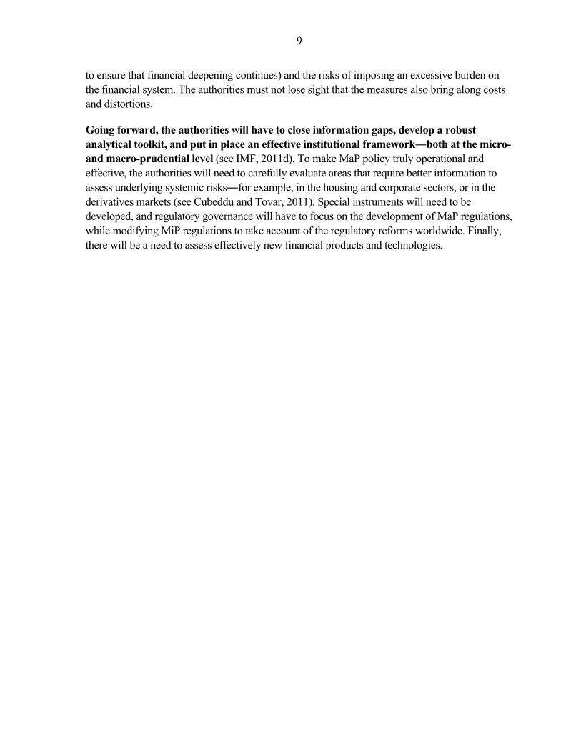
Provisions and capital buffer a bank from credit losses. Provisions can be either general, to account for expected losses in the portfolio that have yet to be identified since they have not realized yet; or specific, to account for losses from specific impaired loans and write-offs. Because ex-ante loss estimates may differ from realized losses a bank holds another buffer, capital, to be able to cover unexpected losses, or losses beyond the mean ex-ante estimate (Figure 1). Clearly, the adequacy of provisions and capital to withstand losses depends on how reliable the estimated loss distribution is.

Figure 1. Capital and Provisions

1 Prepared by Jorge A. Chan-Lau.

Expected loss Unexpected lossCovered by Covered by

Provisions Capital

Losses, Loan portfolio

Pro

bab

ility

of

ob

serv

ing

loss

11

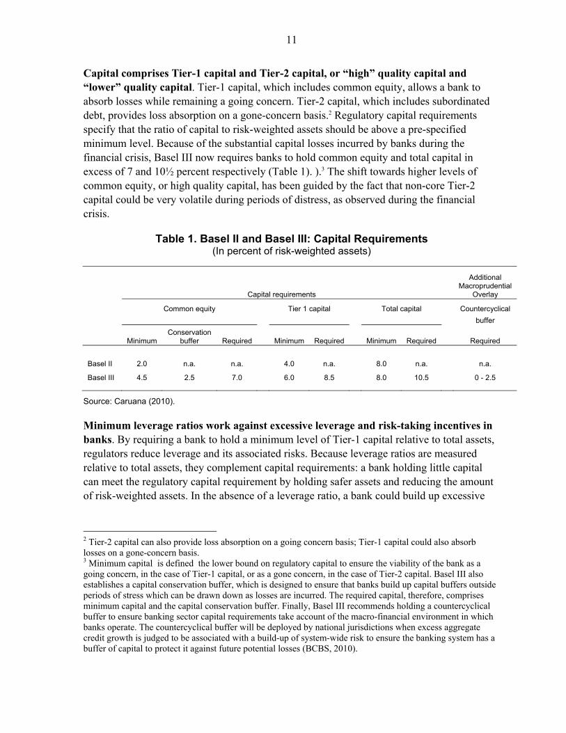
Capital comprises Tier-1 capital and Tier-2 capital, or “high” quality capital and “lower” quality capital. Tier-1 capital, which includes common equity, allows a bank to absorb losses while remaining a going concern. Tier-2 capital, which includes subordinated debt, provides loss absorption on a gone-concern basis.2 Regulatory capital requirements specify that the ratio of capital to risk-weighted assets should be above a pre-specified minimum level. Because of the substantial capital losses incurred by banks during the financial crisis, Basel III now requires banks to hold common equity and total capital in excess of 7 and 10½ percent respectively (Table 1). ).3 The shift towards higher levels of common equity, or high quality capital, has been guided by the fact that non-core Tier-2 capital could be very volatile during periods of distress, as observed during the financial crisis.

Table 1. Basel II and Basel III: Capital Requirements (In percent of risk-weighted assets)

Capital requirements

Additional Macroprudential

Overlay

Common equity Tier 1 capital Total capital Countercyclical

buffer

Minimum Conservation

buffer Required Minimum Required Minimum Required Required

Basel II 2.0 n.a. n.a. 4.0 n.a. 8.0 n.a. n.a.

Basel III 4.5 2.5 7.0 6.0 8.5 8.0 10.5 0 - 2.5

Source: Caruana (2010).

Minimum leverage ratios work against excessive leverage and risk-taking incentives in banks. By requiring a bank to hold a minimum level of Tier-1 capital relative to total assets, regulators reduce leverage and its associated risks. Because leverage ratios are measured relative to total assets, they complement capital requirements: a bank holding little capital can meet the regulatory capital requirement by holding safer assets and reducing the amount of risk-weighted assets. In the absence of a leverage ratio, a bank could build up excessive

2 Tier-2 capital can also provide loss absorption on a going concern basis; Tier-1 capital could also absorb losses on a gone-concern basis. 3 Minimum capital is defined the lower bound on regulatory capital to ensure the viability of the bank as a going concern, in the case of Tier-1 capital, or as a gone concern, in the case of Tier-2 capital. Basel III also establishes a capital conservation buffer, which is designed to ensure that banks build up capital buffers outside periods of stress which can be drawn down as losses are incurred. The required capital, therefore, comprises minimum capital and the capital conservation buffer. Finally, Basel III recommends holding a countercyclical buffer to ensure banking sector capital requirements take account of the macro-financial environment in which banks operate. The countercyclical buffer will be deployed by national jurisdictions when excess aggregate credit growth is judged to be associated with a build-up of system-wide risk to ensure the banking system has a buffer of capital to protect it against future potential losses (BCBS, 2010).

12

leverage even if it complies fully with capital requirements. Basel III proposes a minimum leverage ratio of 3 percent during a trial period from January 2013 to January 2017.

Countercyclical buffers attempt to reduce the buildup of risks during economic booms and financial in the ensuing downturn. Two such measures have featured more prominently in the policy discussion. The first measure, a countercyclical capital buffer, requires banks to build an extra layer of common equity during the upswing of the cycle. The buffer aims to ensure that, in addition to safeguard individual bank solvency, the banking sector in aggregate can help to maintain the flow of credit in the economy during an economic downturn. Basel III proposes a countercyclical capital buffer in the range of 0 to 2½ percent which would be triggered by changes in an aggregate credit indicator. Therefore countercyclical capital buffers would apply system-wide. The second measure, dynamic provisions, requires banks to build up provisions during an economic expansion that would later offset loan losses when the economy slows down or contracts. In contrast to countercyclical capital buffers, dynamic provisions are generally bank-specific and calibrated according to the bank’s lending activity. Both measures could help to dampen excess credit growth during an expansion. The countercyclical capital buffer raises the cost of credit reducing its demand.4 Dynamic provisions, by requiring banks to hold higher provisions, reduce the resources available for funding loans and help restrain credit growth (Box 1).

Box 2.1. Accounting Treatment of Provisions and Capital

Provisions can be either general, to account for expected losses in the portfolio that have yet to be identified since they have not realized yet; or specific, to account for losses from specific impaired loans and write-offs. General provisions are considered appropriations of retained earnings so their increase reduces the capital of the bank. Specific provisions are considered a current expense and can be deducted from taxes. The differential tax treatment provides banks with incentives to minimize general provisions and end under-provisioned relative to expected future losses. Under Basel II, the incentive was partly offset by the allowance to count general provisions towards Tier II capital up to a maximum of 1.25 percent of risk-weighted assets.

______ References: Sunley (2003) and Ryan (2007).

4 The cost of capital of a bank is the weighted average of the cost of equity and the cost of debt. Ceteris paribus, the cost of capital increases when the share of equity increases, which is reflected in higher borrowing costs for the bank’s customers.

13

C. Implications for Latin America

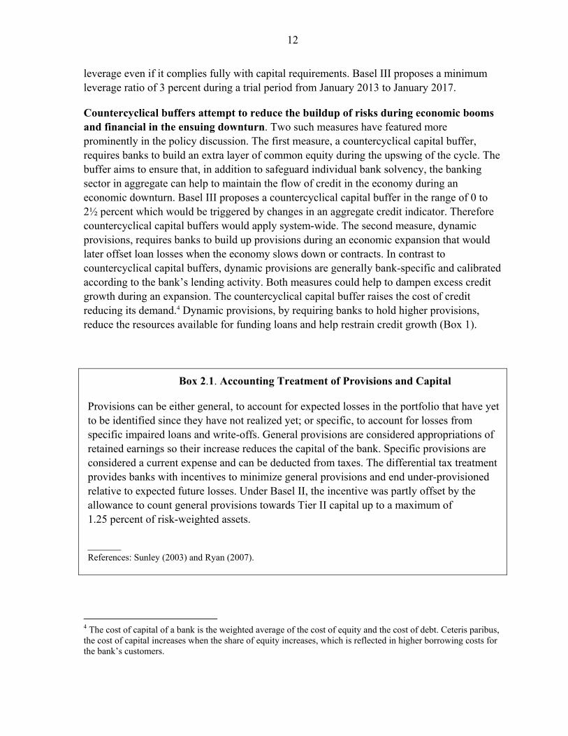
Latin American banks hold higher capital levels and are less leveraged than banks in advanced industrialized countries. The new capital requirements and the minimum leverage ratio proposed by Basel III were designed to address shortcomings of banks in industrialized countries. But Latin American banks appear to exhibit characteristics quite different from their peers in advanced countries. Data for Brazil, Chile, Colombia, Mexico, Peru, and Uruguay show that banks are well capitalized. In general, the common equity to risk-weighted assets ratio in most banks is above the minimum required in Basel III, and in many instances, the ratios also satisfy the required conservation and countercyclical buffers (Figure 2). Similarly, banks have leverage ratios well above the minimum 3 percent proposed in Basel III (Figure 3).5 These findings reflect the prudent stance of the supervisory authorities and reforms in regulation and supervision (Caruana, 2010).

Because Latin America is not immune to boom and bust cycles, dampening procyclicality remains a major policy challenge. In some instances, substantial capital inflows have contributed to excess credit growth in the region and the buildup of credit risk. Because banks appear well capitalized and leverage is low, it could be argued that the main rationale for adopting countercyclical buffers is to “lean against the wind” and reduce procyclicality rather than to enhance bank solvency.

Countercyclical capital buffers, as long as they have a non-negligible impact on the cost of credit, could help to smooth the flow of credit. During the expansionary stage of the cycle, higher capital buffers would increase the cost of credit, i.e. lending spreads, and slowdown the credit expansion. On the other hand, during an economic downturn, the release of the capital buffer, i.e. allowing banks to reduce their capital ratios by the amount of the countercyclical capital buffer, could help to ensure that bank lending is not curtailed drastically.6 Figure 4 shows the sensitivity of lending spreads to increases in the capital ratio, in percentage points, of a representative bank in LA 5 countries.7

5 The calculations are based on banking data, including risk-weighted assets, compiled by the national supervisory agencies using national accounting standards. Common equity was calculated following BCBS (2010d). 6 See Drehmann et al (2010) for details. For a critical assessment of countercyclical capital buffers, see Repullo (2010). 7 The calculations were based on the BCBS methodology described in King (2010), which is similar to that in Elliott (2009) and Kashyap, Hanson, and Stein (2010).

14

Figure 2. Common Equity to Risk-Weighted Assets Ratio Distribution in Selected Latin American Countries1

0

1

2

3

4

5

6

7

8

9

< 4.5 4.5 - 7 7 - 9.5 9.5 - 12 12 - 15 15 - 20 20 - 25 > 250

1

2

3

4

5

6

7

8

9Total number of banks = 25

Common equity to risk-weigthed assets ratio, in percent

0

1

2

3

4

5

6

0

1

2

3

4

5

6

< 4.5 4.5 - 7 7 - 9.5 9 - 12 12 - 15 15 - 20 20 - 25 > 25


Num

ber o

f ba

nks

0

2

4

6

8

10

12

14

< 4.5 4.5 - 7 7 - 9.5 9.5 - 12 12 - 15 15 - 20 20 - 25 > 250

2

4

6

8

10

12



Nu

mbe

r of

ban

ks

0

1

2

3

4

< 4.5 4.5 - 7 7 - 9.5 9.5 - 12 12 - 15 15 - 20 20 - 25 > 250

1

2

3



Num

ber

of b

anks

0

1

2

3

4

5

6

7

0

1

2

3

4

5

6

7

< 4.5 4.5 - 7 7 - 9.5 9.5 - 12 12 - 15 15 - 20 20 - 25 > 25

Total number of banks = 15


Nu

mbe

r of

ban

ks

Sources: Central banks and/or national banking superviosry agencies, and author's calculations.Note: Basel III proposesa minimum common equity to risk-weighted asset ratio of 4.5 percent, augmented to 7 percent to include conservation buffer, and to 9.5 percent after adding a capital buffers and countercyclical capital.1 Data as of June 2010, except for Uruguay (Janaury 2011).

Brazil Chile

Colombia Mexico

Peru Uruguay (private banks only)

N.A.

15

Figure 3. Leverage Ratio Distribution in Selected Latin American Countries

0

2

4

6

8

< 3 3 - 6 6 - 9 9 - 12 12 - 15 15 - 20 20 - 25 > 250

2

4

6


Num

ber

of b

anks

Leverage ratio, in percent

0

2

4

6

8

10

< 3 3 - 6 6 - 9 9 - 12 12 - 15 15 - 20 20 - 25 > 250

2

4

6

8

10

Num

ber o

f ban

ks


0

2

4

6

8

< 3 3 - 6 6 - 9 9 - 12 12 - 15 15 - 20 20 - 25 > 250

2

4

6



Num

ber

of b

anks

0

2

4

6

8

< 3 3 - 6 6 - 9 9 - 12 12 - 15 15 - 20 > 250

2

4

6



Num

ber

of b

anks

Sources: Central banks and/or national banking superviosry agencies, and author's calculations.Note: Basel III proposesa minimum leverage ratio, calculated as Tier-1 capital to total assets, of 3 percent.1 Data as of June 2010, except for Uruguay (Janaury 2011).

Brazil Chile

Colombia Mexico

Peru Uruguay (private banks only)

N.A.

0

2

4

6

< 3 3 - 6 6 - 9 9 - 12 12 - 15 15 - 20 20 - 25 > 250

2

4



Num

ber o

f ban

ks

16

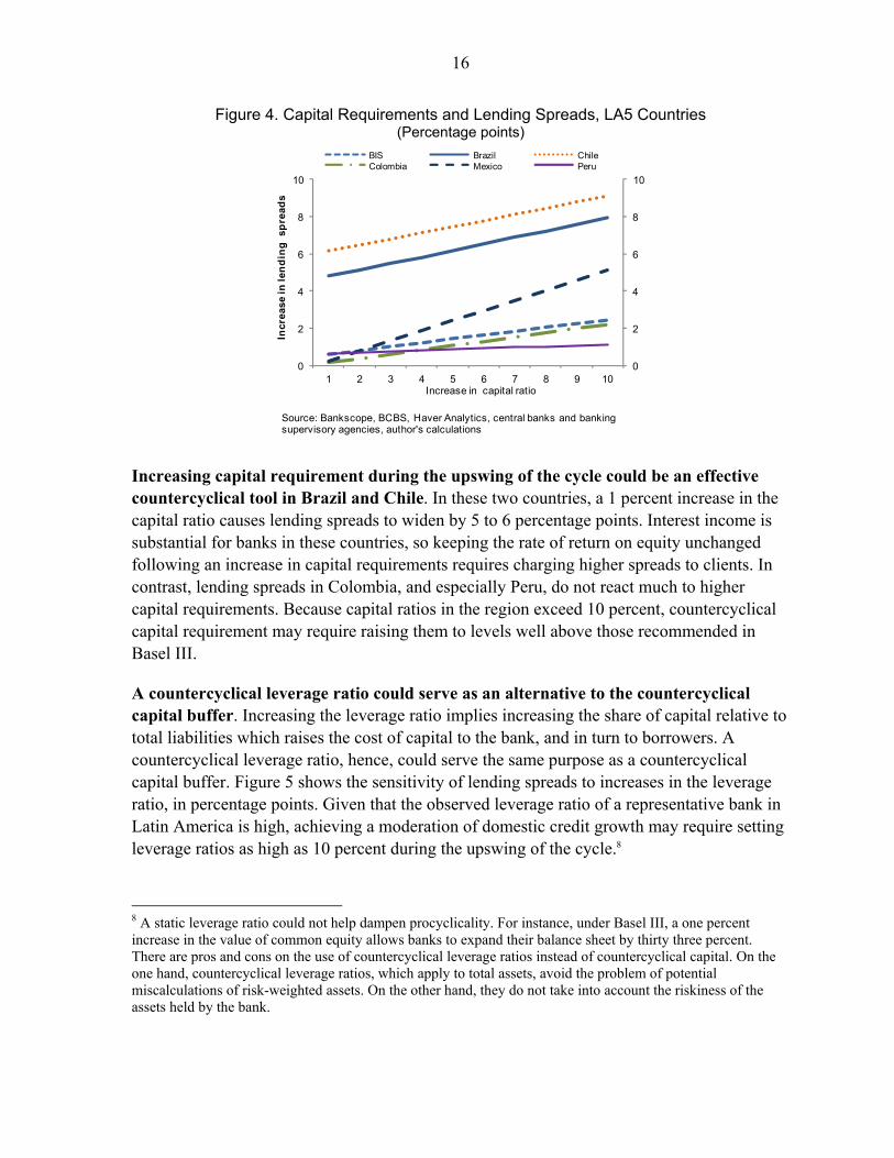
Figure 4. Capital Requirements and Lending Spreads, LA5 Countries (Percentage points)

Increasing capital requirement during the upswing of the cycle could be an effective countercyclical tool in Brazil and Chile. In these two countries, a 1 percent increase in the capital ratio causes lending spreads to widen by 5 to 6 percentage points. Interest income is substantial for banks in these countries, so keeping the rate of return on equity unchanged following an increase in capital requirements requires charging higher spreads to clients. In contrast, lending spreads in Colombia, and especially Peru, do not react much to higher capital requirements. Because capital ratios in the region exceed 10 percent, countercyclical capital requirement may require raising them to levels well above those recommended in Basel III.

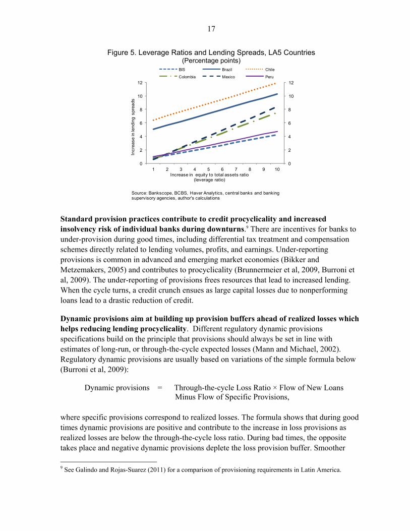
A countercyclical leverage ratio could serve as an alternative to the countercyclical capital buffer. Increasing the leverage ratio implies increasing the share of capital relative to total liabilities which raises the cost of capital to the bank, and in turn to borrowers. A countercyclical leverage ratio, hence, could serve the same purpose as a countercyclical capital buffer. Figure 5 shows the sensitivity of lending spreads to increases in the leverage ratio, in percentage points. Given that the observed leverage ratio of a representative bank in Latin America is high, achieving a moderation of domestic credit growth may require setting leverage ratios as high as 10 percent during the upswing of the cycle.8

8 A static leverage ratio could not help dampen procyclicality. For instance, under Basel III, a one percent increase in the value of common equity allows banks to expand their balance sheet by thirty three percent. There are pros and cons on the use of countercyclical leverage ratios instead of countercyclical capital. On the one hand, countercyclical leverage ratios, which apply to total assets, avoid the problem of potential miscalculations of risk-weighted assets. On the other hand, they do not take into account the riskiness of the assets held by the bank.

0

2

4

6

8

10

0

2

4

6

8

10

1 2 3 4 5 6 7 8 9 10

Incr

ease

in l

end

ing

sp

read

s

Increase in capital ratio

BIS Brazil ChileColombia Mexico Peru

Source: Bankscope, BCBS, Haver Analytics, central banks and banking supervisory agencies, author's calculations

17

Figure 5. Leverage Ratios and Lending Spreads, LA5 Countries (Percentage points)

Standard provision practices contribute to credit procyclicality and increased insolvency risk of individual banks during downturns.9 There are incentives for banks to under-provision during good times, including differential tax treatment and compensation schemes directly related to lending volumes, profits, and earnings. Under-reporting provisions is common in advanced and emerging market economies (Bikker and Metzemakers, 2005) and contributes to procyclicality (Brunnermeier et al, 2009, Burroni et al, 2009). The under-reporting of provisions frees resources that lead to increased lending. When the cycle turns, a credit crunch ensues as large capital losses due to nonperforming loans lead to a drastic reduction of credit.

Dynamic provisions aim at building up provision buffers ahead of realized losses which helps reducing lending procyclicality. Different regulatory dynamic provisions specifications build on the principle that provisions should always be set in line with estimates of long-run, or through-the-cycle expected losses (Mann and Michael, 2002). Regulatory dynamic provisions are usually based on variations of the simple formula below (Burroni et al, 2009):

Dynamic provisions = Through-the-cycle Loss Ratio × Flow of New Loans Minus Flow of Specific Provisions,

where specific provisions correspond to realized losses. The formula shows that during good times dynamic provisions are positive and contribute to the increase in loss provisions as realized losses are below the through-the-cycle loss ratio. During bad times, the opposite takes place and negative dynamic provisions deplete the loss provision buffer. Smoother

9 See Galindo and Rojas-Suarez (2011) for a comparison of provisioning requirements in Latin America.

0

2

4

6

8

10

12

0

2

4

6

8

10

12

1 2 3 4 5 6 7 8 9 10

Incr

ease

in le

ndin

g s

prea

ds

Increase in equity to total assets ratio(leverage ratio)

BIS Brazil Chile

Colombia Mexico Peru

Source: Bankscope, BCBS, Haver Analytics, central banks and banking supervisory agencies, author's calculations

18

profits work against procyclicality, and the build-up of provisions consistent with through-the-cycle estimates reduce the probability of failure of banks during a downturn.10 Besides Spain, a number of Latin American countries have already adopted regulatory dynamic provisions (Box 2).

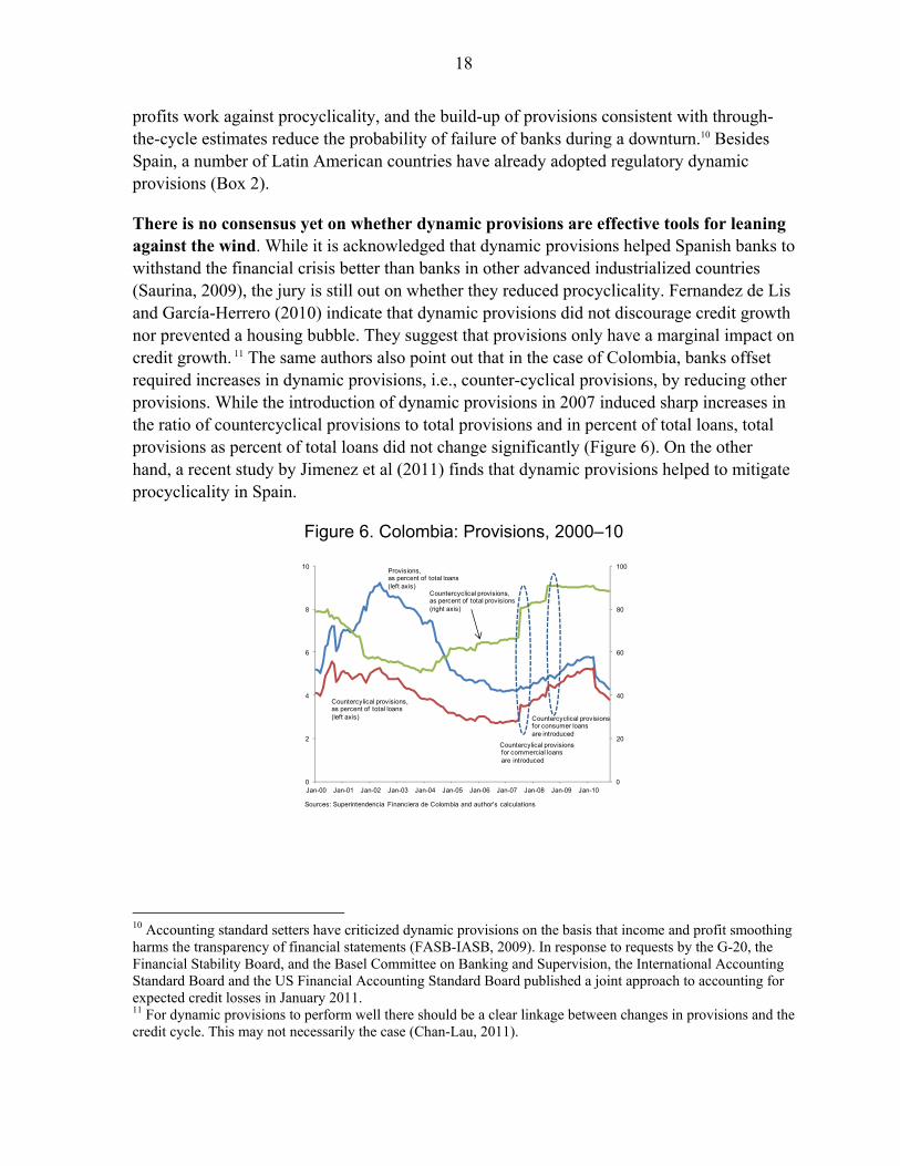
There is no consensus yet on whether dynamic provisions are effective tools for leaning against the wind. While it is acknowledged that dynamic provisions helped Spanish banks to withstand the financial crisis better than banks in other advanced industrialized countries (Saurina, 2009), the jury is still out on whether they reduced procyclicality. Fernandez de Lis and García-Herrero (2010) indicate that dynamic provisions did not discourage credit growth nor prevented a housing bubble. They suggest that provisions only have a marginal impact on credit growth. 11 The same authors also point out that in the case of Colombia, banks offset required increases in dynamic provisions, i.e., counter-cyclical provisions, by reducing other provisions. While the introduction of dynamic provisions in 2007 induced sharp increases in the ratio of countercyclical provisions to total provisions and in percent of total loans, total provisions as percent of total loans did not change significantly (Figure 6). On the other hand, a recent study by Jimenez et al (2011) finds that dynamic provisions helped to mitigate procyclicality in Spain.

Figure 6. Colombia: Provisions, 2000–10

10 Accounting standard setters have criticized dynamic provisions on the basis that income and profit smoothing harms the transparency of financial statements (FASB-IASB, 2009). In response to requests by the G-20, the Financial Stability Board, and the Basel Committee on Banking and Supervision, the International Accounting Standard Board and the US Financial Accounting Standard Board published a joint approach to accounting for expected credit losses in January 2011. 11 For dynamic provisions to perform well there should be a clear linkage between changes in provisions and the credit cycle. This may not necessarily the case (Chan-Lau, 2011).

0

20

40

60

80

100

0

2

4

6

8

10

Jan-00 Jan-01 Jan-02 Jan-03 Jan-04 Jan-05 Jan-06 Jan-07 Jan-08 Jan-09 Jan-10

Provisions,as percent of total loans(left axis)

Countercyclical provisions,as percent of total provisions(right axis)

Countercylical provisions,as percent of total loans(left axis)

Countercylical provisionsfor commercial loansare introduced

Countercyclical provisionsfor consumer loans are introduced

Sources: Superintendencia Financiera de Colombia and author's calculations

19

Box 2.2. Dynamic Provisions in Spain and Latin America Spain The Spanish dynamic provisions formula builds general provisions that accounts for expected losses in new loans extended in a given period and the expected losses on the outstanding stock of loans at the end of that period after netting off specific provisions incurred during the period. If new loans of an homogeneous category k are denoted by ∆ , general provisions, , should be increased by the amount of ∆ where should be representative of the average credit losses during a business cycle of loans in category k. This first component is an incremental provision that account for expected losses in new loans. Banks also have to hold an amount of specific provisions reflecting the average specific provisions made during the business cycle but that have not been realized yet. This amount is equal to , where is the average specific provision for loans in category k and is the outstanding amount of loans. Finally, the specific provisions component should be corrected for specific provisions already incurred during the period, . Provisions accumulate according to the formula below: ∑ ∆ , where the different loan categories, and the choice of parameters in the formula above are determined by the banking regulatory agency. There are six different loan groups or categories in ascending order of risk: negligible risk, low risk, medium-low risk, medium-risk, medium-high risk, and high risk. The general provision parameters, or alpha-parameters, corresponding to these groups are 0, 0.6, 1.5, 1.8, 2, and 2.5 percent respectively; and the specific provision parameters, or beta-parameters, are 0, 0.11, 0.44, 0.65, 1.1, and 1.64 percent respectively. The system also specifies that cumulative provisions should not exceed 125 percent of the inherent losses of the loan portfolio, ∑ . Reference: Saurina (2009). Bolivia Banks are required to maintain a dynamic provision in the range of 1½ to 5½ percent of total loans, depending on the type of loan: 1½ percent for mortgage loans, 1.6 percent for microfinance loans; 2.3 percent for consumer loans and prime corporate loans; and between 3.2 percent and 5.5 percent for subprime corporate loans. Banks can access the provision stock to offset up to half of the additional specific provisions required in a given month provided that the loan quality has deteriorated for six consecutive months and the dynamic provision has been phased in fully). Reference: Wezel (2010). Colombia Colombia adopted dynamic provisions for commercial and consumer loans in 2007. Banks can measure the credit risk of the loans using either the regulatory reference model or approved proprietary models. The regulatory model establishes three types of tax-deductible provisions: individual, countercyclical, and general provisions. General provisions should exceed 1 percent of the total loan portfolio, and can be used to meet countercyclical provisions. Countercyclical provisions cover credit risk from changes in the borrower’s creditworthiness due to changes in the economic cycle. Both individual and countercyclical provisions are accounted under the same item. In the reference model, individual provisions are calculated based on expected losses under a regulatory baseline scenario. During periods of rapid growth, countercyclical provisions are calculated as the difference between expected losses in a more adverse scenario and the baseline scenario. During

20

Box 2.2. Dynamic Provisions in Spain and Latin America (continued) periods of slow growth, countercyclical provisions are not required. Finally, banks can use countercyclical provisions at the discretion of the regulator to compensate for increases in individual provisions during an economic downturn. Reference: Fernandez de Lis and Garcia Herrero (2010). Peru The countercyclical provisioning rule requires Peruvian banks to build up additional minimum provisions whenever the rule is activated by one of the conditions below: a) the annualized average percent change of GDP during the past 30 months reaches or exceeds

5 percent from below; b) the annualized average percent change of GDP during the past 30 months is above 5 percent and

the average annualized percent change of GDP during the past 12 months exceeds by 2 percentage points its value one year before;

c) the annualized average percent change of GDP during the past 30 months is above 5 percent and 18 months have elapsed since the rule was deactivated by second deactivation condition.

Countercyclical provisions are deactivated by one of the two conditions below: a) the annualized average percent change of GDP during the last 30 months falls to or below 5

percent; b) the annualized average percent change of GDP during the last 12 months is lower by at least 4

percentage points than its value one year before. The minimum countercyclical provision is 0.4 percent for corporate clients, 0.45 percent for large enterprises; 0.3 percent for medium-sized corporates; 0.50 percent for small and micro-corporates; 1.5 percent and 1 percent for revolving and nonrevolving consumer loans respectively, and 0.4 percent for mortgage loans. Reference: SBS, 2008, Resolución S.B.S. No. 1356, November 19. Uruguay Dynamic provisions were introduced in 2001. The regulation specifies that banks contribute to their individual dynamic provisioning funds, DPt, the difference between the monthly statistical net losses on loans to the nonfinancial private sector (NFPS) and the realized net loan loss in that month:

∆DP ∑ α C LL ,

The statistical losses are derived by multiplying 1/12 of the expected rate of loss for five loan categories, ranging from 0.1 percent for low-risk loans to 1.8 percent for credit card loans, by the respective loan volumes, Ct. The net loan loss, LLt, incurred in a given period is calculated as the cost of additional specific provisions recorded in the profit and loss statement, net of deactivations of specific provisions (i.e., reclassifications of loans toward higher categories) and recoveries of defaulted loans already written off. At the inception of dynamic provisioning, the beta parameters were reportedly distributed around the average annual loan loss during 1990-2000, which was 1 percent of loans. The dynamic provisions fund of each bank is bounded between 0 and 3 percent of total loans to be provisioned. Reference: Wezel (2010).

21

System-wide dynamic provisions triggered by changes in aggregate economic activity could prove more effective for restraining credit growth. Although more prudent banks are penalized, system-wide provisions would force all banks to increase provisions regardless of whether they are expanding their lending activity. Such provisioning system has been in place in Peru since 2008. Dynamic, countercyclical provisions in excess of general and specific provisions are required when the growth of economic activity exceeds a regulatory threshold, usually set at the growth rate of potential output, or if the year-on-year growth accelerates rapidly. The countercyclical provisions requirement is deactivated when economic growth falls below potential or the economy slows down substantially (see Box 2).

D. Conclusions

Countercyclical capital requirements and leverage ratios could help restrain excessive credit growth in Latin America by raising the cost of capital. In the case of capital flows-driven credit growth, these measures could complement other macroprudential tools like LTV limits and reserve requirements and facilitate the conduction of monetary and fiscal policy. Nonetheless, using these countercyclical tools may require raising capital requirements and leverage ratios well above the levels recommended in Basel III. The effectiveness of these tools could be impaired if a substantial share of the flow of credit is channeled outside the banking system, or if banks are willing to accept a lower return on equity rather than passing the increased cost of capital to borrowers.

System-wide dynamic provisions triggered by changes in aggregate economic activity could reduce procyclicality. Peru implemented such system in 2008 and it is rather early to assess its performance as provision buffers have only started to build up recently. Nonetheless, the fact that system-wide dynamic provisions lean against the wind as countercyclical capital buffers allows extrapolating the findings from BCBS (2010c). The findings suggest that countercyclical buffers triggered by aggregate indicators could do a good job in reducing procyclicality.12 It should be bear in mind, however, that provisions based on aggregate indicators could impair efficiency and competition in the banking system (Fernandez de Lis and García-Herrero, 2010).

Regardless of whether aggregate or bank-specific variables trigger dynamic provisions, their success depends on reliable estimates of long-run expected loss and a balance between rules and discretion. Estimating long-run expected losses remains a formidable challenge. For instance, in Peru expected loss estimates are based on the banking crisis experienced in the 1990s, which some argue it is too conservative and may put domestic banks at disadvantage vis-à-vis other credit providers. In dynamic provision regimes, calibration relies on past historical data and it may fail to capture the dynamics of expected losses going forward and should be complemented with discretionary judgment. Reaching

12 But see Repullo (2010) for arguments against the effectiveness of countercyclical buffers.

22

the adequate balance between rules and discretion remains a challenge (Ocampo, 2003, Turner Review, 2009, Griffith-Jones and Ocampo with Ortiz, 2009).

23

III. LIQUIDITY REQUIREMENTS FOR MACROPRUDENTIAL PURPOSES1

This note describes the main features and effects of the new policies based on liquidity ratios that adjust for stress scenarios. In particular, the note reviews the Basel III liquidity requirements. In addition, Annex 1 discusses recent selected country experiences with similar measures in Australia, Colombia, Chile, and New Zealand.

A. Motivation

There is agreement that illiquidity amplified the depth and severity of the global crisis and needs more attention (IMF, 2011a and 2010a; Gorton and Metrick, 2010; Shin, 2010; or Brunnermeir, 2009). The excess reliance on wholesale and cross border funding, which are less stable funding alternatives, contributed to the inability of multiple financial institutions to roll-over financial needs during the crisis (IMF, 2010a). Furthermore, excessive leverage in the financial system and short-term foreign debt have been identified as main determinants of sharp output collapses in emerging markets (Blanchard et al., 2010 and Berkman et al., 2009).

Liquidity risk management has become a regulatory priority, both from a micro and macro prudential angle. Its goals are to build up liquidity buffers and improve the structure and resilience of funding in banks and the financial system as a whole. Thus, by making banks and the system more resilient to a downturn, and by minimizing the adverse effects of runoffs and fire sales, liquidity risk managements can help reduce systemic risk. Furthermore, since liquidity regulations may increase the cost of funding they may also help dampen the credit cycle in the upswing. Achieving these goals involves identifying, measuring, monitoring and controlling liquidity risk. More generally, it requires ensuring stable funding sources, generating predictable flow of funds, reducing asset/liability maturity mismatches, and avoiding spillovers across the financial system.

Liquidity is the ability of a bank to fund increases in assets and meet obligations as they come due without incurring unacceptable losses (BCBS (2008) or Brunnermeir (2009)). Liquidity risk materializes if the institution is unable to convert assets into cash, or fails to procure enough funding.2 Even, if funding is available, it may be too costly, thus affecting the institution’s current and future stream of incomes and capital.

The concept of liquidity has various dimensions: funding liquidity, market liquidity and liquidity crisis. Funding liquidity is the ability to raise cash (or cash equivalents) either borrowing or through the sale of an asset; Market liquidity relates to the ability to trade an

1 Prepared by Camilo E. Tovar. Comments by J. Chan-Lau, C. Fernández, G. Terrier, and R. Valdés are acknowledged. 2 Liquid securities should have certain properties such as being short term, backed by diversified portfolios, and immune from adverse selection when traded i.e. information-insensitive. However, notice that in episodes of liquidity crisis, information-insensitive debt can become information sensitive (Gorton and Metrick, 2010).

24

asset or financial instrument at short notice with little impact on its price. This is turn can take several forms: tightness, depth, immediacy, and resilience. Tightness refers to the difference between buy and sell prices, e.g., bid-ask spreads. Depth refers to the size of transactions that can be executed without altering the price. Immediacy refers to the speed at which orders can be executed, and resilience to the ease with which prices return to normal after temporary disturbances. Finally, a sudden and prolonged evaporation of both market and funding liquidity may have systemic consequences for the stability of the financial system leading to “liquidity crisis” or “systemic liquidity shortfalls” (IMF, 2011a). These are often episodes in which agents’ endogenous responses generate an unwillingness to bear risk, i.e., “liquidity black holes” (Shin, 2010).

Policy makers can manage idiosyncratic and systemic liquidity risks by imposing limits over traditional liquidity indicators and managing them in a countercyclical manner whenever necessary.3 For instance this is the case with traditional liquidity,4 core funding, noncore funding, or leverage ratios. Additional tools such as reserve requirements on deposits can also been employed (IMF, 2010b and Garcia et al, 2011). 5 At the systemic level, new methodologies are only recently being proposed, but work is required in this area (see IMF, 2011a).

Traditionally, liquidity ratios have been measured under normal circumstances rather than under stressed conditions. To address this shortcoming, some countries (e.g., New Zealand and Colombia) have improved the monitoring and control tools of liquidity risk, extending them to include crisis-like stress scenarios. The new Basel III framework has also complemented the global regulatory banking standards with a set of stressed liquidity requirements: the Liquidity Coverage Ratio (LCR) and Net Stable Funding Ratio (NSFR).6

Despite their usefulness, a more formal macroprudential framework is required to deal with systemic liquidity risk. Indeed, although the measures covered in this note should help strengthen liquidity management and the funding structure of individual banks―thus enhancing the stability of the banking sector―they are microprudential in nature. They are not designed to mitigate systemic liquidity risks where the interaction of financial institutions can result in the simultaneous inability of institutions to access sufficient liquidity and funding liquidity under stress. Under such circumstances a regulation that would charge and

3 Liquidity provision at the international level is as aspect that is not considered here. Nonetheless, important advances have been made including, for instance, the mechanisms such as the IMF Flexible Credit Line (FCL). 4 Indicators that gauge the capacity of assets easily converted into cash to cover banks liabilities (e.g., current or quick liquidity ratios). 5 Liquidity requirements can also be linked to the degree of currency mismatches and its maturity. For instance, Mexico imposes a liquidity requirement to address short-term and medium term liquidity concerns that are linked to the currency mismatch and, which is also adjusted by the remaining maturity of this mismatch (see Banco de Mexico’s Circular 2019). 6 The BCBS(2010a,b,c and 2009a,b) has outlined other metrics for monitoring liquidity risk, including a contractual maturity mismatch, concentration funding, available encumbered assets, the LCR by currency, and a market-related tool for monitoring liquidity with little or no time lag (BCBS 2010a).

25

institution for its contribution to systemic liquidity risk becomes more evident. However, robust methodologies for measuring systemic liquidity risk are only being proposed at this stage (IMF, 2011a).

B. The Liquidity Coverage Ratio (LCR)

The LCR is as tool to make banks less susceptible to potential short-term disruptions in accessing funding. Specifically, its goal is to ensure banks have liquidity to survive one month of stressed funding conditions. Therefore the LCR identifies the amount of unencumbered (i.e. not pledged and not held as a hedge for any other exposure), high quality, liquid assets that can be employed to offset expected cash outflows over a 30-day horizon (Table A.1). The ratio of these two components must exceed 100 percent. The LCR will be in observation starting in 2011, and will be introduced as a minimum standard in 2015.

Its main components are: a stress-test scenario, the definition of high quality assets, and the bank’s expected cash outflow over a one-month period (see Annex Table A.1 for details).

The stress scenario considers a downgrade in the institution’s credit rating, a run-off of retail deposits, disruptions in secure and unsecured funding capacity, disruption in the market that affect the quality of collateral, and unscheduled draws on credit and liquidity facilities. Of course, banks are expected to have their own stress tests to assess the level of liquidity they should hold beyond this minimum supervisory requirement.

The high liquid assets must guarantee a liquidity-generating capacity in periods of severe idiosyncratic, either by selling the asset or through secured borrowing, and in case of severe market stress they should be eligible for operations by central banks (e.g., overnight facilities). They also must satisfy fundamental, market, and operational features that allow them to be easily and immediately converted into cash at little or no loss value. The stocks of liquid assets that satisfy the previous characteristics are then weighted according to their liquidity.7

Finally, the net expected cash flow is difference between cumulative expected cash outflows and cumulative expected cash inflows in the specified stress test scenario in the period under consideration. In other words, it is the net cumulative liquidity mismatch position under stress measured at the test horizon. The cumulative expected cash outflow multiplies outstanding balances of various categories or types of liabilities and off-balance sheet commitments by rates at which they are expected to run off or be drawn down. The cumulative expected cash inflow multiply outstanding

7 The LCR is expected to be met and reported in a single currency, but banks should meet liquidity needs in each currency. Thus a LCR by currency is expected to be monitored and reported to track currency mismatches.

26

balances of various categories of contractual receivables by rates at which they are expected to flow under the stress scenario up to an 75 percent of total expected cash outflows.

C. Net Stable Funding Ratio (NSFR)

The NFSR has been introduced as a complement to the LCR with the goal of addressing longer-term structural maturity liquidity mismatches in banks balance sheets. It promotes medium and long-term bank funding by setting a minimum acceptable amount of “stable funding” based on the liquidity characteristics of a bank’s assets over a one-year horizon.8 The NSFR will be introduced in 2018 after an observation period starting in 2011.

The NSFR is defined as the ratio between available stable funding and required stable funding. Its main components are the stress scenario and the definitions of stable, available, and required funding. Operationally stable funding sources are given greater weight, while assets that require funding are adjusted by a factor (or haircut) depending on their expected liquidation value. Once taken this into account the ratio must exceed 100 percent (see Annex Table A.2 for details).

The stress scenario considers a significant decline in profitability or solvency arising from heighted credit, market or operational risk, or other risk exposures; a downgrade in debt, counterparty credit or deposit rating by a nationally recognized credit rating organization; and an event which calls into question the reputation or credit quality of the institution. Extended borrowing from the central bank lending facilities outside regular open market operations are not considered in the ratio.

The stable funding includes those types and amounts of equity and liability financing expected to be reliable sources of funding over one-year horizon under conditions of stress. The available stable funding (ASF) is defined as the total amount of capital; preferred stock with maturity greater than one year; secured and unsecured borrowings and liabilities (including deposits) with effective maturities of one year or greater; proportion of stable wholesale funding, nonmaturity deposits, and/or term deposits with maturities of less than one year expected to stay with the institution for an extended period in an idiosyncratic stress event. The ASF assigns the carrying value of an institution’ equity and liabilities to one of five categories and then multiplies it by a weighting factor.

Finally, the required stable funding (RSF) for assets and off-balance sheet exposures is measured using supervisory assumptions on the broad characteristics of the liquidity risk profiles of an institution’s assets, off-balance sheet exposures and

8 In Brazil (and probably some other emerging markets), medium and long term funding may imply higher FX risks (issuance of bonds abroad).

27

selected activities. It is calculated as the sum of assets held and funded by the institution and off-balance sheet activity (or potential liquidity exposure) each of which is adjusted by a factor. The factor aims at capturing the amount of the asset that cannot be monetized through sale or use of collateral in a secured borrowing on an extended basis during a liquidity event lasting one year.

D. Quantitative and Economic Impact of LCR and NSFR

Because banks have different alternatives to accommodate and fulfill the proposed liquidity requirements, evaluating their economic impact is not straightforward. The LCR and NSFR will force some banks to lengthen their term funding. This might lead to an increase in the average spread charged on the entire loan portfolio. Intuitively, average interest rates spreads may widen as liquidity requirements force banks to shift away from cheap short term funding and towards more expensive but stable longer term funding. To maintain profitability (i.e., return on equity) banks are likely to compensate for the higher operational costs by increasing the average spread charged on their entire loan portfolio. Credit supply may also decline, in particular long term, as banks find fulfilling the maturity mismatch more costly.

Evidence shows that a significant number of banks in the BCBS member countries have liquidity shortfalls and will have to lengthen the maturity of their short- and long-term funding (BCBS, 2010b). In particular, the BCBS reports an average LCR of 83 percent for large banks and 98 percent for the remaining banks in its sample by end 2009. This implies a liquidity shortfall of EUR 1.7 trillion for the system. The NSFR for the same group of banks was 93 and 103 percent, respectively, an estimated shortfall of stable funding of EUR 2.9 trillion. These estimates are in line with those found by the IMF in a recent study (IMF, 2011a).

The cost to meet the NSFR is sensitive to the definition of the ratio, assumptions about the composition of banks’ assets and liabilities, and estimates of the returns of different assets and the costs of different liabilities. This information is not disclosed in banks’ financial statements. However, a sense of the costs involved is provided by a recent study that uses the data collected by the BCBS for its Quantitative Impact Study. According to it, banks will have to increase average lending spreads by 24 bps for banks to converge to the required NSFR (King, 2010). The study also finds that the spread declines to 12 bps or less when additional measures adopted in Basel III are included. The reason is that holding higher quality investment lowers the risk weighted assets and, thus capital adequacy requirements.

There are concerns about the ability of the NSFR to signal failures due to liquidity problems. Although it is recognized that the NSFR may have some capacity to signal future liquidity problems, evidence suggests that it would have done so inconsistently prior to the 2007–08 crisis (IMF, 2011a). Although, estimates show that the average NSFR worsened in 2008―slightly falling below 0.95―and improved slightly in 2009; and that liquidity problems surfaced in half of the banks with a NSFR ratio below 80 percent.; its weakness

28

arises because failed banks are found to be evenly distributed across the range of estimated NSFRs for a cross-section of 60 globally oriented banks in 20 countries and three regions (Europe, North America, and Asia).

E. Conclusions

Liquidity requirements are a fundamental microprudential policy tool that can contribute to minimize systemic risk. These measures should improve the resilience of individual institutions and minimize liquidity systemic risks. On the one hand, they help improve the funding structures of banks in good times, thus reducing their exposure to unforeseen liquidity shocks (e.g., fire sales) or to spillovers that may arise in turbulent market times. On the other hand, they can reduce the procyclicality of the financial cycle by increasing the cost of funding. As such, liquidity requirements can be a useful complement to help contain financial and economic excess under the current external financial conditions.

More generally, stressed liquidity requirements help with the identification, measurement, monitoring, and control of liquidity risk. In this regard, the Basel III liquidity framework i.e. the LCR and NSFR, along with the BCBS “Principles for sound liquidity risk management and supervision” (BCBS, 2008) provide a minimum standard for liquidity risk and sets a higher standard for bank-specific analysis, governance, and supervision.

The experiences with liquidity risk frameworks in Australia, Colombia and New Zealand are practical avenues for the immediate implementation of policies aiming at identification, measure, monitor, and control of liquidity risk under stress conditions (see Annex).

Although the impact of these requirements are moderate, the evidence suggests that larger banks are more likely to be affected, rather than smaller ones which tend to be funded with deposits.9 On average these measures are likely to lead to a moderate increase in average interest rates. In the case of New Zealand funding costs relative to the policy rate increased by an equivalent policy tightening of 100–150 basis points. Whatsoever their final impact will depend on its interaction with other measures, including those of Basel III.

More generally, it must be kept in mind that the liquidity requirements describe here are microprudential in nature, and are not specifically designed to address systemic risk. As such, a framework to mitigate system wide, or systemic risk, is highly desirable. However, developing such framework is not straight forward. In the mean time, a well calibrated LCR and NSFR would contribute to the liquidity and funding stability of banks. Nonetheless, to minimize systemic risk, special consideration will have to be taken as to whether these requirements should vary over the cycle or across institutions.

9 However, in some EMEs this funding structure may not apply. In Brazil, for instance, large banks rely more on deposits than smaller banks.

29

Finally and looking forward, it is important to examine mechanisms to deal with liquidity risks that could take place outside the regulatory perimeter, and how to ring-fence the core financial system from problems arising outside the perimeter. In this respect, more work is required to strengthen the disclosure of detailed information on various liquidity risk measures inside and outside the financial system.

30

Annex 1. Country Experiences: New Zealand, Colombia, Chile, and Australia

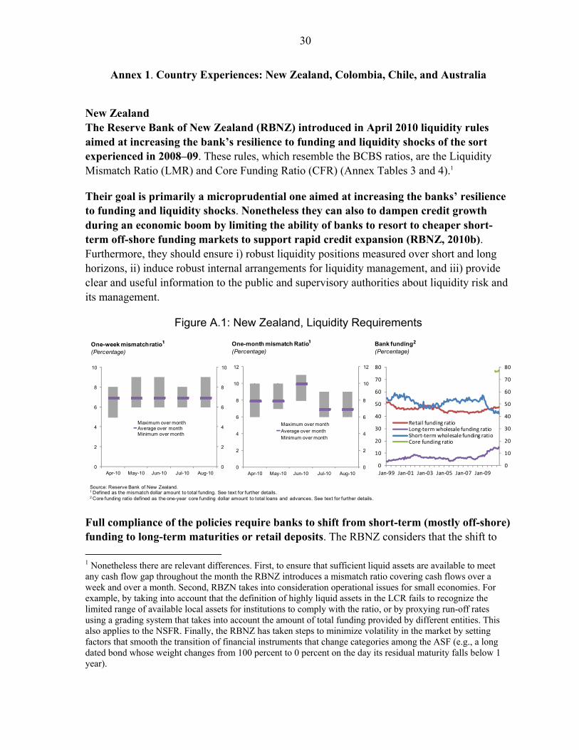
New Zealand The Reserve Bank of New Zealand (RBNZ) introduced in April 2010 liquidity rules aimed at increasing the bank’s resilience to funding and liquidity shocks of the sort experienced in 2008–09. These rules, which resemble the BCBS ratios, are the Liquidity Mismatch Ratio (LMR) and Core Funding Ratio (CFR) (Annex Tables 3 and 4).1

Their goal is primarily a microprudential one aimed at increasing the banks’ resilience to funding and liquidity shocks. Nonetheless they can also to dampen credit growth during an economic boom by limiting the ability of banks to resort to cheaper short-term off-shore funding markets to support rapid credit expansion (RBNZ, 2010b). Furthermore, they should ensure i) robust liquidity positions measured over short and long horizons, ii) induce robust internal arrangements for liquidity management, and iii) provide clear and useful information to the public and supervisory authorities about liquidity risk and its management.

Figure A.1: New Zealand, Liquidity Requirements

Full compliance of the policies require banks to shift from short-term (mostly off-shore) funding to long-term maturities or retail deposits. The RBNZ considers that the shift to

1 Nonetheless there are relevant differences. First, to ensure that sufficient liquid assets are available to meet any cash flow gap throughout the month the RBNZ introduces a mismatch ratio covering cash flows over a week and over a month. Second, RBZN takes into consideration operational issues for small economies. For example, by taking into account that the definition of highly liquid assets in the LCR fails to recognize the limited range of available local assets for institutions to comply with the ratio, or by proxying run-off rates using a grading system that takes into account the amount of total funding provided by different entities. This also applies to the NSFR. Finally, the RBNZ has taken steps to minimize volatility in the market by setting factors that smooth the transition of financial instruments that change categories among the ASF (e.g., a long dated bond whose weight changes from 100 percent to 0 percent on the day its residual maturity falls below 1 year).

0

2

4

6

8

10

0

2

4

6

8

10

Apr-10 May-10 Jun-10 Jul-10 Aug-10

Maximum over monthAverage over monthMinimum over month

One-week mismatch ratio¹(Percentage)

Source: Reserve Bank of New Zealand.1 Defined as the mismatch dollar amount to total funding. See text for further details.2 Core funding ratio defined as the one-year core funding dollar amount to total loans and advances. See text for further details.

0

2

4

6

8

10

12

0

2

4

6

8

10

12

Apr-10 May-10 Jun-10 Jul-10 Aug-10

Maximum over monthAverage over monthMinimum over month

One-month mismatch Ratio¹(Percentage)

0

10

20

30

40

50

60

70

80

0

10

20

30

40

50

60

70

80

Jan-99 Jan-01 Jan-03 Jan-05 Jan-07 Jan-09

Retail funding ratioLong-term wholesale funding ratioShort-term wholesale funding ratioCore funding ratio

Bank funding2

(Percentage)

31

longer-term funding will tend to increase lending rates (10–20 bps) for any given policy rate depending on the difference in spreads between short- and long-term wholesale funding and how those funding spreads change through the cycle. Nonetheless evidence shows that their announcement increased the banks’ willingness to pay more to attract retail deposits.2 As a result bank funding costs relative to the policy rate increased by an equivalent policy tightening of 100bps, which in turn led to an increase in lending rates relative to benchmark rates (Box 1.9 in IMF, 2010d and Jang, 2010).

Currently all banks in the system comply with the minimum liquidity requirements. Indeed, the LMR are well above the regulatory minimum of zero. They also hold comfortable funding buffers which exceed the current minimum requirements for the CFR of 65 percent as well as the expected new requirement of 75 percent (Figure A.1 and Annex Table 4).3

Colombia The Colombian supervisory authority introduced in April 2009 a liquidity risk management system (SARL due to its name in Spanish).4 The system aims at identifying, measuring, controlling, and monitoring liquidity risk in the trading book and on and off credit institutions’ balance sheet. The system defines a liquidity risk weekly reporting standard of mandatory compliance with no mandatory limits (Annex Table 5). However, credit institutions and upper-level financial cooperatives may design a system with their own models as long as they are consistent with the guidelines set by the supervisory authority.

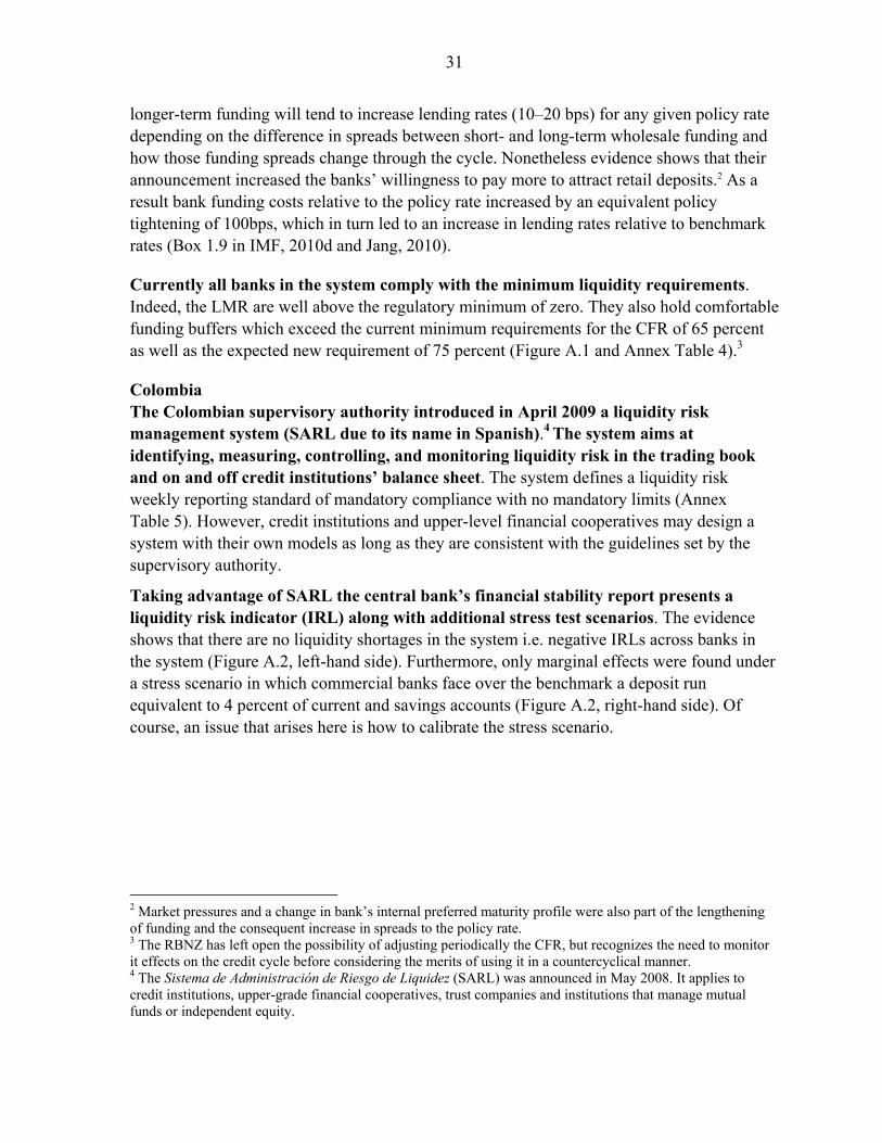
Taking advantage of SARL the central bank’s financial stability report presents a liquidity risk indicator (IRL) along with additional stress test scenarios. The evidence shows that there are no liquidity shortages in the system i.e. negative IRLs across banks in the system (Figure A.2, left-hand side). Furthermore, only marginal effects were found under a stress scenario in which commercial banks face over the benchmark a deposit run equivalent to 4 percent of current and savings accounts (Figure A.2, right-hand side). Of course, an issue that arises here is how to calibrate the stress scenario.

2 Market pressures and a change in bank’s internal preferred maturity profile were also part of the lengthening of funding and the consequent increase in spreads to the policy rate. 3 The RBNZ has left open the possibility of adjusting periodically the CFR, but recognizes the need to monitor it effects on the credit cycle before considering the merits of using it in a countercyclical manner. 4 The Sistema de Administración de Riesgo de Liquidez (SARL) was announced in May 2008. It applies to credit institutions, upper-grade financial cooperatives, trust companies and institutions that manage mutual funds or independent equity.

32

Figure A.2: Colombia, Liquidity Risk Indicator

Chile In its most recent Financial Stability Report, the Central Bank of Chile calculates some approximations of the LCR and NSFR. Its findings show that the Chilean banking system exceeds the minimum requirements (Central Bank of Chile, 2010). It is worth noticing that these estimates have been disclosed despite regulations being based on Basel I.

Australia The LCR requires financial institutions to hold a large enough stock of high quality liquid assets––normally marketable securities such those issued by governments or by low risk corporate––to offset net cash flows over a 30-day time period. However, for different reasons (e.g., fiscal prudence) these securities are in short supply in Australia.5 To address this situation the Basel III incorporates alternative treatments for the holding of liquid assets. One option is to allow banking institutions to establish a contractual committed liquidity facility provided by the central bank—subject to a fee—that would count toward the LCR requirement.

5 The LCR defines to categories of high quality liquid assets: Level 1 and Level 2 (see Annex Table 1). APRA has reviewed the range of marketable instruments denominated in Australian dollars against the Basel III criteria for high-quality liquid assets. The review has taken into account the amount of the instrument on issue, the degree to which the instrument is broadly or narrowly held, and the degree to which the instrument is traded in large, deep and active markets. APRA has given particular attention to the liquidity of the instrument during the market disruptions of the global financial crisis. Based on this review, APRA has determined that, as of February 2011 the only assets that qualify as Level 1 assets are cash, balances held with the Reserve Bank of Australia, and Commonwealth Government and semi-government securities; and there are no assets that qualify as Level 2 assets.

0.0

0.2

0.4

0.6

0.8

1.0

1.2

1.4

1.6

0.0

0.2

0.4

0.6

0.8

1.0

1.2

1.4

1 2 3 4 5 6 7 8 9 10 11 12 13 14 15 16 17 18

24-sep-10 26-Nov-10 28-Jan-11

Liquidity risk indicator¹(Percentage)

Source: Banco de la Republica.Note: Horizontal axis correspond to indiidual banks.1 Ratio of the liquidity gap and total assets ajusted for market liquidity. See text for further details. Execise performed on January 10,2011.2 The stress scenario is a deposit run of 4% of current and savings accounts. See text for further details.

0.0

0.1

0.2

0.3

0.4

0.5

0.6

0.7

0.8

0.0

0.1

0.2

0.3

0.4

0.5

0.6

0.7

0.8

1 2 3 4 5 6 7 8 9 10 11 12 13 14 15 16 17 18

7 days Non-stressed 7 days stressed

Liquidity risk indicator: Stress test exercise1,2

(Percentage)

33

The Reserve Bank of Australia (RBA) and the Australian Prudential Regulation Authority (APRA) decided on December 2010 that an authorized deposit-taking institution (ADI) would be able to establish a committed secure liquidity facility with the RBA. This facility would be sufficient in size to cover any shortfall between the ADI’s holdings of high-quality liquid assets and the LCR requirement. The qualifying collateral for the facility will comprise all assets eligible for repurchase transactions with the RBA under normal market operations.

The RBA will charge a market-based commitment fee on all institutions who have established a facility with the Bank (i.e. those ADIs to which the Bank has made a funding commitment). This market-based fee will be designed to provide institutions with broadly the same incentives to prudently manage their liquidity as their counterparts in jurisdictions where there is ample supply of high quality liquid assets in their domestic currency. However further details about the design of the fee have yet to be determined. Only the larger ADIs (around 40) will be eligible for the facility and will have to demonstrate to APRA that all steps have been taken to meet their LCR requirements through their own balance sheet management before relying on the RBA facility. The details of the RBA liquidity facility and APRA's prudential standard on liquidity risk management will be subject to consultation during 2011 and 2012.

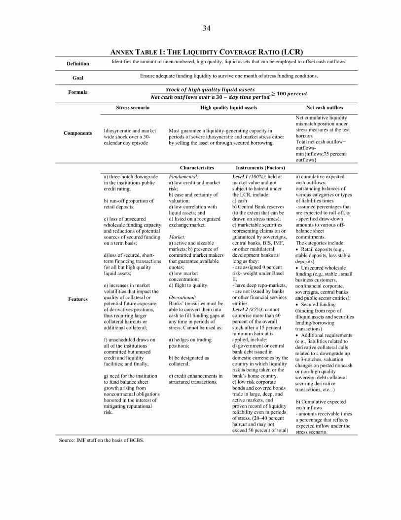
34

ANNEX TABLE 1: THE LIQUIDITY COVERAGE RATIO (LCR) Definition Identifies the amount of unencumbered, high quality, liquid assets that can be employed to offset cash outflows.

Goal Ensure adequate funding liquidity to survive one month of stress funding conditions.

Formula

Components

Stress scenario High quality liquid assets Net cash outflow

Idiosyncratic and market wide shock over a 30-calendar day episode

Must guarantee a liquidity-generating capacity in periods of severe idiosyncratic and market stress either by selling the asset or through secured borrowing.

Net cumulative liquidity mismatch position under stress measures at the test horizon. Total net cash outflow= outflows-min{inflows;75 percent outflows}

Features

Characteristics Instruments (Factors)

a) three-notch downgrade in the institutions public credit rating; b) run-off proportion of retail deposits; c) loss of unsecured wholesale funding capacity and reductions of potential sources of secured funding on a term basis; d)loss of secured, short-term financing transactions for all but high quality liquid assets; e) increases in market volatilities that impact the quality of collateral or potential future exposure of derivatives positions, thus requiring larger collateral haircuts or additional collateral; f) unscheduled draws on all of the institutions committed but unused credit and liquidity facilities; and finally, g) need for the institution to fund balance sheet growth arising from noncontractual obligations honored in the interest of mitigating reputational risk.

Fundamental: a) low credit and market risk; b) ease and certainty of valuation; c) low correlation with liquid assets; and d) listed on a recognized exchange market. Market: a) active and sizeable markets; b) presence of committed market makers that guarantee available quotes; c) low market concentration; d) flight to quality. Operational: Banks’ treasuries must be able to convert them into cash to fill funding gaps at any time in periods of stress. Cannot be used as: a) hedges on trading positions; b) be designated as collateral; c) credit enhancements in structured transactions.

Level 1 (100%): held at market value and not subject to haircut under the LCR, include: a) cash b) Central Bank reserves (to the extent that can be drawn on stress times); c) marketable securities representing claims on or guaranteed by sovereigns, central banks, BIS, IMF, or other multilateral development banks as long as they: - are assigned 0 percent risk- weight under Basel II, - have deep repo-markets, - are not issued by banks or other financial services entities. Level 2 (85%): cannot comprise more than 40 percent of the overall stock after a 15 percent minimum haircut is applied, include: d) government or central bank debt issued in domestic currencies by the country in which liquidity risk is being taken or the bank’s home country. e) low risk corporate bonds and covered bonds trade in large, deep, and active markets, and proven record of liquidity reliability even in periods of stress. (20–40 percent haircut and may not exceed 50 percent of total)

a) cumulative expected cash outflows: outstanding balances of various categories or types of liabilities times -assumed percentages that are expected to roll-off, or - specified draw-down amounts to various off-balance sheet commitments. The categories include: Retail deposits (e.g., stable deposits, less stable deposits). Unsecured wholesale funding (e.g., stable , small business customers, nonfinancial corporate, sovereigns, central banks and public sector entities). Secured funding (funding from repo of illiquid assets and securities lending/borrowing transactions) Additional requirements (e.g., liabilities related to derivative collateral calls related to a downgrade up to 3-notches, valuation changes on posted noncash or non-high quality sovereign debt collateral securing derivative transactions, etc...) b) Cumulative expected cash inflows - amounts receivable times a percentage that reflects expected inflow under the stress scenario.

Source: IMF staff on the basis of BCBS.

35

ANNEX TABLE 2: NET STABLE FUNDING RATIO (NSFR) Definition Addresses maturity mismatches between assets and liabilities.

Goal Set a minimum acceptable amount of stable funding based on the liquidity characteristics of a bank’s assets over a one-year horizon.

Formula

Components

Stress Scenario Stable Funding

extended over one year firm-specific stress scenario

Types and amounts of equity and liability financing expected to be reliable sources of funding over one-year horizon under conditions of extended stress.

Features

Available Stable Funding Required Stable Funding

Factor Item Factor Item a) significant decline in profitability or solvency arising from heighted credit, market or operational risk, or other risk exposures; b) a downgrade in a debt, counterparty credit or deposit rating by nationally recognized credit rating organization; c) a material event which calls into question the reputation or credit quality of the institution. Extended borrowing from the central bank lending facilities outside regular open market operations are not considered in the ratio.

100%

i) capital (tier 1 and 2); ii) preferred stock (not in tier 2) with maturity equal to or greater than one year; iii) Secured and unsecured borrowings and liabilities (including deposits) with effective maturities of one year or greater. iv) Total amount of secured and unsecured borrowings and liabilities (including term deposits) with effective maturities of one year or greater

0%

i) Cash, money market instruments, securities and outstanding loans to financial entities with effective remaining maturities of less than a year.

90%

v) “Stable” nonmaturity (demand) deposits and/or term deposits with residual maturities of less than one year provided by retail customers and small business customers.

5%

ii) Unencumbered assets with maturities of more than one year representing claims on AA-graded or higher grades and assigned 0 percent risk weight under Basel II standardized approach.

80%

vi) “Less stable” nonmaturity (demand) deposits and/or term deposits with residual maturity of less than one year provided by retail customers and small business customers.

20%

iii) Unencumbered corporate bonds rated at least AA or marketable securities with maturities of more than one year which are traded in deep, active and liquid markets.

50%

vii) Unsecured wholesale funding, nonmaturity deposits and/or term deposits with a residual maturity of less than a year provided by nonfinancial corporates.

50%

iv)Gold; v) Unencumbered equity securities listed on a major exchange and included in a large capital market index and unencumbered corporate bonds rated AA- to A- with maturities of more than one year which are traded in deep, active and liquid markets. vi) Loans to non-financial corporate clients having a residual maturity of less than one year.

0%

vii) All other liabilities and equity categories.

65%

vii) Unencumbered residential mortgages (of any maturity) and other loans on more than a year qualifying for the 35 percent or lower risk weight in Basel II standardized approach for credit risk.

85%

vii) Loans to retail clients having a residual maturity less than one year.

100% viii) All other assets.

Source: IMF staff on the basis of BCBS.

36

ANNEX TABLE 3: NEW ZEALAND––LIQUIDITY MISMATCH RATIOS (LMR) Goal Increase bank’s resilience to liquidity shocks by requiring banks to maintain sufficient cash and liquid assets to

maintain short-term funding requirements.

Definition Maintain a mismatch ratio that is no less than the minimum specified at the end of each business day.

Indicator one-week mismatch ratio (OWMR) one-month mismatch ratio (OMMR)

Formula

100 100

Requirement 0 percent

Components

One-week mismatch dollar amount = primary liquid assets after accounting for haircuts + 75 percent of undrawn committed lines to the bank available within one week1 - 100 percent of market funding withdrawable at sight or with residual contractual term within one week – nonmarket funding withdrawable at sight or with residual contractual term within one week2 – other contractual outflows due within one week––15 percent of the undrawn balance of committed lines granted by the bank drawable within one week3

One-month mismatch dollar amount = primary liquid assets after accounting for haircuts + secondary liquid assets after accounting for haircuts+contractual inflows due within one month+ 75 percent of undrawn committed lines to the bank available within one month1 - 100 percent of market funding withdrawable at sight or with residual contractual term within one month – nonmarket funding withdrawable at sight or with residual contractual term within one month2– other contractual outflows due within one month––15 percent of the undrawn balance of committed lines granted by the bank drawable within one month3

Source: IMF staff on the basis of RBZN. Note: Ratio is consistent with the BCBS’s Liquidity Coverage Ratio. 1 Up to a maximum amount from any other provider of 3 percent of total’s bank funding; and a maximum amount from all providers together of 9 percent of the bank’s total funding. 2 Applying increasing percentages depending on the size. 3 Other than revolving facilities.

ANNEX TABLE 4: NEW ZEALAND - CORE FUNDING RATIO (CFR) Goal Increase bank’s resilience to funding shocks by requiring banks to maintain sufficient cash and liquid assets to

maintain short-term funding requirements.

Definition Requires banks to hold its one-year core funding ratio at not less than the minimum specified at the end of each business day.

Formula 100

Requirement 65 percent on initial implementation, but it will increase to 75 percent in stages over time, after a review process.

Components

One-year core funding dollar amount = all funding with residual maturity longer than one year1 + 50 percent of any tradable debt securities issued by the bank with original maturity of two years or more and with residual maturity at the reporting date of more than six months and not more than a year + non-market funding that is withdrawable at sight or with residual maturity less than or equal to a year, applying decreasing percentages that decline with the size of the fund tier 1 capital.

Source: IMF staff on the basis of RBZN. Note: Ratio is consistent with the BCBS’s Net Stable Funding Ratio. 1 Including subordinated debt and related party funding.

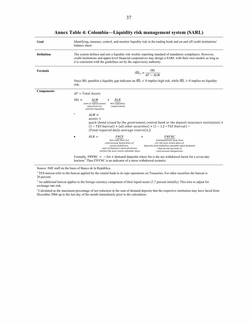
37

Annex Table 4: Colombia––Liquidity risk management system (SARL)

Goal Identifying, measure, control, and monitor liquidity risk in the trading book and on and off credit institutions’ balance sheet.

Definition The system defines and sets a liquidity risk weekly reporting standard of mandatory compliance. However, credit institutions and upper-level financial cooperatives may design a SARL with their own models as long as it is consistent with the guidelines set by the supervisory authority.

Formula

Since IRL parallels a liquidity gap indicator an IRL 0 implies high risk, while IRL 0 implies no liquidity risk.

Components

, 1 1 1.2

1,2

, ,

Formally, FNVNC frn demand deposits where frn is the net withdrawal factor for a seven-day horizon.3 Thus FNVNC is an indicator of a stress withdrawal scenario.

Source: IMF staff on the basis of Banco de la República. 1 TES-haircut refer to the haircut applied by the central bank to its repo operations on Treasuries. For other securities the haircut is 20 percent. 2 An additional haircut applies to the foreign currency component of their liquid assets (3.7 percent initially). This tries to adjust for exchange rate risk. 3 Calculated as the maximum percentage of net reduction in the sum of demand deposits that the respective institution may have faced from December 2006 up to the last day of the month immediately prior to the calculation.

38

IV. DEBT TO INCOME LIMITS1

The global financial crisis has highlighted that households, like corporations and financial institutions, are highly indebted, particularly in some of the countries that have been at the center of this crisis. This raises many questions about the sustainability of households’ indebtedness and the interconnectedness of balance sheets. It also makes it necessary to consider policy actions to address this indebtedness. This note discusses the degree of household indebtedness, its implications, and a possible action to address household indebtedness, namely the implementation of debt to income limits.

A. Debt to Income Ratios

Households are highly indebted in many advanced countries, some of which have been at the center of the global financial crisis. Table 1 shows that the ratio of gross household debt to GDP ranged from 129 percent in Ireland to 50 percent in Italy in 2010 (IMF, 2011a). The ratio of gross household debt to GDP was 91 percent and 107 percent in the United States the United Kingdom, respectively, two countries that have been at the focal point of the crisis. The ratio of gross household debt to GDP was nearly 93 percent in Canada, among the highest in this group of countries. Tempering these high ratios is the fact that households’ debt is far less than households’ holdings of financial assets. The ratio of net household debt to GDP (i.e., debt minus financial assets) was minus 230 percent in the United States and minus 184 percent in the United Kingdom. Undoubtedly, the large household holdings of financial assets have implications about the ongoing debate about the role of collateral in the extension of credit.

Table 1. Household Indebtedness in Selected Advanced Economies (Percent of 2010 GDP, unless noted otherwise)

Figures published by the Banque de France confirm the high indebtedness of households in countries that were at the center of the crisis (Table 2). These figures, which rely on different sources than the ones used to compile the gross household debt to GDP in Table 1, show that the gross household debt to GDP were highest in the United States, the United Kingdom, and Spain. The figures for the gross household debt to

1 Prepared by Carlos Medeiros. This note has benefited from comments by and conversations with Reinout De Brock, Diane Mendoza, Camilo Tovar, other members of the WHD Macroprudential Working Group, and colleagues throughout the Fund.

Belgium Canada Euro Area France Germany Greece Ireland Italy Japan Portugal Spain U.K. U.S.

Households Gross Debt1 54.8 92.8 72.4 69.4 61.5 68.2 129.0 50.4 74.0 103.4 90.1 106.5 91.1

Households Net Debt1 2 -204.3 … -129.2 -131.3 -130.4 -55.7 -60.2 -177.7 -231.5 -126.1 -73.8 -183.9 -230.1

Source: IMF, 2011.1 Most recent data divided by 2010 GDP. 2 Household net debt is calculated using financial assets from a country's flow of funds.

39

disposable income (DI) were also highest in the United States, United Kingdom, and Spain. As of end-September 2010, the figures for gross household debt to DI reached 149 percent in the United States, 142 percent in the United Kingdom, and 126 percent in Spain. In the context of the global financial crisis, these figures would seem to suggest that a high ratio of gross household debt to DI could be a source of major source of risk to economic stability. As Mian and Sufi (2010) note, the increase in household leverage in the United States explains well the rise in mortgage defaults, and the subsequent fall in house prices and decline in durable goods consumption. Stated differently, the deleveraging of households therefore appears to have contributed to the sharp retrenchment in economic growth in the United States.

Table 2. Household Indebtedness in Selected Advanced Economies

B. Risks Arising from Household Indebtedness

Households face increasing risks as their indebtedness rises. As the experience in the global financial crisis has shown, households that borrow too much, or borrow in excess of their ability to repay, could end up facing payment obligations that are unsustainable. Households may simply not have enough disposable income to meet their obligations and could also experience a sudden decline, or worse a loss of income, or an increase in essential spending needs, which would make it difficult, if not impossible, to meet their debt obligations. In the context of an economic crisis that results in an increase in unemployment and a decrease in wealth, including the value of homes, this could have severe consequences for households. In addition, changes in credit conditions, for example as a result of an increase in interest rates that leads to an increase in payments on variable-interest loans, or a credit crunch, would make it difficult to roll over debt obligations. The interaction of these risks could be particularly difficult to manage (Elul et al. 2010).

A generalized inability by households to service their debt could pose a systemic risk for the economy. As the crisis has shown, the inability of households to repay their obligations could jeopardize the health of financial institutions, and, in the case of extreme shocks, have systemic consequences (Dynan, 2009; Mayer et al., 2009). This could adversely impact the ability of financial institutions to extend credit, which could negatively affect businesses’ capacity to continue with their ongoing investment projects or to kick off new projects. Depending on the extent of these difficulties, the government may see its finances deteriorate as a result of a decline in tax revenue and possibly its balance sheet weaken because of the need to support financial institutions in difficulty. Such developments would, no doubt, have

GDP DI GDP DI GDP DI GDP DI GDP DI GDP DI GDP DI GDP DI

30-Mar-09 123.6 156.9 66.1 100.6 63.3 93.9 63.5 89.3 51.8 75.2 42.7 61.5 85.2 124.5 100.4 145.731-Dec-09 122.5 155.0 66.5 100.4 64.1 94.6 63.5 89.3 52.8 76.0 43.8 62.8 85.8 124.3 101.0 145.4

30-Sep-10 117.0 148.8 64.4 96.2 64.3 95.8 61.9 88.3 53.9 77.2 44.3 64.1 85.0 125.7 98.3 142.0

Source: Banque de France.

U.K.U.S. Japan Eurozone Germany France Italy Spain

40

an adverse impact on economic growth. In this light, the key question is: Is there a policy that could limit the risks arising from a generalized problem of household indebtedness?

C. Debt to Income Limits

DTI limits could help reduce the risks associated with high household indebtedness, while lessening the procyclicality in lending. Implementing DTI limits could help reduce the households’ debt-service payment difficulties, or lessen the probability of default. In doing so, these limits could also help lower the likelihood of the materialization of the systemic risk arising from the generalized inability of households to service their debt. These limits could be preventive in nature. At the same time, DTI limits could contribute to lessen the procyclicality of lending. They could serve to smooth the credit dynamics in the context of the business cycles, by tightening them in the upswings to slow credit expansion and relaxing them in the downswings to spur credit growth.

DTI limits could take on different characteristics. As Chang (2010) and Crowne et al. (2011) note, DTI limits aim at establishing a maximum percentage of a household’s income for paying debt (both principal and interest) in any one year. While the DTI limits could include only a narrow definition of debt such as mortgage obligations, they could also take into account a broad definition of debt, including taxes, insurance fees, or even utilities. The DTI limits could take the form of front-end ratios, which establish the percentage of income for paying housing costs (principal and interest, hazard insurance premium, property taxes, and homeowners’ association fees). The DTI limits could also be back-end ratios, which set the percentage of gross income for paying all recurring debt payments (Galati and Moessner, 2011). Finally, DTI limits could be either discretionary or rules based subject to credit dynamics.

The effectiveness of DTI limits would depend on several factors. First, the effectiveness of DTI limits, as with any other tool to reduce the incidence of future crises, would depend on supervisory enforcement of the limits. This would require the issuance of guidelines, regulations or laws to lay the basis for the application of DTI limits, and the creation of a comprehensive database on household debt and income to track such limits. Second, the effectiveness of these limits would depend on how well financial institutions use them to assess the creditworthiness of borrowers, which, in the case of households, focuses on past debt payment record, indebtedness, income, wealth, and collateral (Tirole, 2006). While financial institutions may well face increased costs for including the DTI limits in the assessment of creditworthiness of households, they need to weigh this increase in costs against the potential decline in the costs of collecting late debt-service payments or going through bankruptcy procedures. Third, the effectiveness of such limits would also require the participation of all financial institutions that extend credit to households. Households should not have the ability to pick financial institutions with a view to avoiding the DTI limits.

41

Many countries worldwide have actively used DTI limits. More than two dozen countries, including some in Latin America, require financial institutions to use DTI limits as part of their assessment of creditworthiness of households. By way of example, the United States has long used DTI limits for conventional loans and mortgage loans insured by the Federal Housing Administration. In the case of conventional loans, the DTI limits have typically been 28/36 percent. The 28 percent is applied to the housing payment, and the 36 percent is applied to the housing payment plus recurring debt. Hong Kong SAR has put in place caps on debt service to income as a condition for household lending. As part of their efforts to improve financial institutions’ risk management, lower FX credit risk and protect borrowers, particularly in the low-income groups, Poland and Serbia have put in place differentiated debt-service to income limits by currency. The fact that other countries have not used these limits may well reflect the difficulty in determining household income, particularly in economies that still face high degree of informality, and the lack of consolidated household debt

Korea has made DTI limits part of its discretionary policy tools. In 2005, Korea adopted DTI limits as part of a package of policy actions for the real estate sector aimed at increasing the supply of housing, lowering housing prices, and restructuring the property tax system. In adopting this package, Korea also sought to limit speculation in the real estate sector. Korea initially set the DTI limits at 40 percent for married borrowers whose spouse already had a mortgage and for unmarried applicants 30 years or younger seeking houses in areas that had seen sharp house price increases (e.g., speculative areas). However, later Korea began to apply differentiated lending limits within a range of 40 percent to 60 percent depending on the size of the housing unit, lending amount, borrower’s credit rating, repayment method, interest rate, and evidence of income. After introducing the DTI limits in August 2005, Korea tightened the DTI limits on seven occasions and loosened them on one occasion.

A study shows that a tightening of the DTI limits in Korea has important results (Igan and Kang, forthcoming). Preliminary econometric results in this study show that a tightening of the DTI limits results in a slowdown or even a reversal of house price increases six months after the intervention. At the same time, a tightening of the DTI limits leads to a decline in transaction activities in the housing industry over many months following the intervention, particularly in metropolitan areas. The econometric results suggest that the tightening of the DTI limits has more of an impact on transaction activities than on house prices. The tightening of the DTI limits also results in some deceleration of the growth of household debt levels. Finally, the study concludes that a tightening of the DTI limits may be helpful to curb price expectations in the housing sector.

Still, the use of DTI limits requires further analysis. The determination of the DTI limits, including whether to apply them to credit lines or contingent liabilities, needs careful consideration. The interaction of DTI limits and other leverage ratios, including the debt to liquid net worth ratio, and collateral requires further analysis. In this context, it is necessary to consider whether households that provide significant collateral, say, in the form of liquid

42

financial assets, to borrow should be subject to the same DTI limits as households that do not provide collateral or provide collateral that is not liquid. In addition, the definition of the debt and income used to determine the DTI limits also requires careful analysis. For instance, should the debt include only mortgages or all debt? Should income exclude extraordinary income in any one year? Should the determination of DTI limits make use of household debt and income for just one year or should it rely on debt and income over a number of years to smooth out years of extraordinary earnings?

D. Conclusion

High indebtedness of households could heighten systemic risk. High indebtedness jeopardizes the ability of households to service their debt, particularly in the face of major external shocks as observed in the global financial crisis, and makes balance sheets in the economy more fragile. This makes it necessary to consider, among other policies, the use of DTI limits. DTI limits aim at preventing the excessive indebtedness of households, and lessening of procyclicality in lending. As the experience of Korea indicates, limits on the DTI ratio―complemented with other measures―could serve as a credit cycle and countercyclical moderation tool. Kyung-Hwan and Man (2010) note that DTI limits, as with the loan-to-value rate, have proven to be an effective measure for cooling off-housing demand and containing housing price increases in this country.

43

V. LOAN-TO-VALUE RATIO CAPS AS A MACROPRUDENTIAL TOOL1

A. Introduction

Loan-to-value ratio (LTV) caps limit borrowers’ leverage in asset purchases. LTV restrictions set an upper limit to the amount of loan a borrower can take out from the lender to purchase an asset, which usually serves as the collateral of the loan. The restrictions—typically expressed as a percent of the value of the purchased asset or collateral—are often applied to the housing market, though they are also sometimes imposed in other asset markets (e.g., auto loans). In the housing market—where the asset prices are highly procyclical—the denominator of the restrictions often refers to the lower of the market value and the professional surveyor’s assessment value, which tends to fluctuate less along the cycle.

Such limits could be a useful policy tool to help moderate the asset and credit cycles, and mitigate risks to the financial system. While banks are likely to have risk management mechanisms in place that implicitly restrict LTVs, such internal control may become too loose during booms, thus giving rise to the need for an appropriate regulatory limit. LTV caps can create frictions on either leg of the cycle, which often features strong feedback loops between loan growth and asset price/demand dynamics. On the upturn, by dampening the former, a tight LTV cap could also put a drag on the latter. On the downturn, the presence of LTV limits during the preceding boom could reduce defaults and hence banking stress—for instance, in the housing market a lower LTV ratio would imply fewer incidences of negative home equity for any given decline in house price, and there is evidence that those households still with positive home equity are less likely to default (e.g., Bhutta et al., 2010, and Wong et al., 2004).2

B. LTV Rule Implementation3

Targeted focus and transparency are main advantages of LTV restrictions vis-à-vis other tools in addressing asset cycles. LTV rules have first-order influence on credit expansion in the targeted sectors, while leaving the economy-wide liquidity and cost of credit largely unaffected. In addition, since LTV restrictions bind only for new and highly leveraged (hence likely riskier) asset purchases, they entail few “collateral damages”—existing borrowers and less leveraged buyers are not directly affected. They also convey very simple and transparent signals to the public of the authorities’ concerns about asset and credit bubbles.

1 Prepared by Man Keung Tang. This note has benefited from comments from various members of the group. 2 See also the simulation of a financial accelerator model in IMF (2008), which shows that macro procyclicality increases with LTV ratio. 3 Annex 1 on a case study of Hong Kong SAR highlights some practical considerations in LTV rule implementation, and also discusses the effects of the recent LTV tightening there.

44

Implementation of LTV caps can take various forms, notably in a countercyclical fashion to lean against swings in credit supply and asset demand. In particular, many countries have recently either started imposing LTV caps or tightened the existing restrictions as part of their broader toolkit to manage the ongoing upswing.4 To yield sharper focus on specific pressure points in the market, LTV caps can also be applied differentially to loans of different characteristics—e.g., for mortgages, owner-occupied vs. buy-to-lets, high-end vs. lower-priced, “hot” vs. peripheral locations, local currency vs. FX mortgages, and longer duration vs. shorter-term loans. In some cases, there are active government-supported programs that provide mortgage insurance, with which borrowers are allowed a limited breach of the LTV caps (e.g., Canada, Hong Kong SAR).

And often LTV rules are complemented with other regulatory measures to address concerns beyond the degree of leverage. For example, LTV caps on mortgages are sometimes applied along with ceilings on debt servicing to income ratio (DTI) to limit risks from borrowers’ cash flow stress (e.g., Korea, Hong Kong SAR), and/or with higher stamp duty to discourage “flipping” and speculation (e.g., Singapore, Hong Kong SAR).

The use and effectiveness of LTV restrictions, however, is sometimes constrained by practical issues. As with other macroprudential tools, measurement difficulty and potential loopholes give rise to implementation challenges. For instance, high LTV loans may migrate to the parts of the financial sector that are beyond the authorities’ direct prudential oversight (including offshore banks). LTV rules may also be evaded through backdoor arrangements of additional loans disguised as personal loans from banks, or “top-ups”. The targeted nature of the tool—while an advantage—could also create unintended spillovers by pushing financial excess to nontargeted sectors. Moreover, there is not a well-developed analytical framework underpinning the calibration of LTV restriction in accordance with the market’s cyclical position—the recent rapid reversal of housing policy stance in Korea illustrates the difficulty faced by policymakers in determining an appropriate level of LTV limits.5 The relative quantitative arbitrariness could further compound the inherent tension between an adoption of LTV restrictions in the housing market and the socio-political agenda of promoting home ownership in some countries (including through mortgage interest tax deductibility). And from an efficiency perspective, too-strict LTV caps could unduly reduce welfare by erring too much on the side of ensuring stability at the expense of financial deepening.

In light of the constraints and also reflecting a preference against absolute limits, many regulators opt to discourage, rather than strictly rule out, high LTVs. In particular, instead of instituting a LTV cap, some countries apply higher capital charges or provisioning 4 See Annex 2 for some recent examples of LTV rule application. 5 The Korean authorities tightened LTV restrictions in the second half of 2009 to stem the fast rising housing prices; but as the housing cycle turned soon after, the authorities reversed policy stance in August 2010, introducing stimulating measures to support the cooling housing market (e.g., suspending DTI limits for owner-occupied properties until March 2011, subsidizing first-time home buyers, and reducing transaction taxes on some properties).

45

requirements to mortgage loans of higher LTVs (e.g., Norway, Switzerland, the UK, Spain, and Israel). And in some cases, tight LTV limits are applied to only mortgages that are used as collaterals of covered bonds (e.g., Peru, Germany, and Switzerland).

C. Existing Evidence on Effectiveness

Despite their prevalence, the empirical literature on the effectiveness of LTV restrictions is relatively limited, albeit growing. Gerlach and Peng (2005) show that following the introduction of housing LTV caps, credit expansion in Hong Kong SAR has become less sensitive to property prices, hence implying possibly less pronounced credit cycles. Similarly, in a panel of (mostly) advanced economies, Almeida et al. (2006) find that the sensitivity of housing prices and mortgage credit to income shocks is lower when the LTV limits are tighter. Meanwhile, Crowe et al. (forthcoming) find that maximum LTV limits are positively correlated with house price appreciation between 2000 and 2007 in a cross-section of countries, and Wong et al. (2011) show that banks in those countries that have explicit LTV restrictions seem more shielded from house price and macro developments. Using micro survey data, Igan and Kang (forthcoming) find that Korea’s LTV policy—along with many other measures—might have helped moderate the housing cycle by influencing households’ expectations of future house price increase, although the policy’s net social benefits are not assessed. However, the scattered pieces of favorable evidence notwithstanding, there has yet to be a full agreement on the tool’s effectiveness—of those authorities having employed LTV caps, some are convinced of the tool’s usefulness, while others report mixed analytical results, not least reflecting the empirical difficulty of identifying the various factors simultaneously at work (CGFS, 2010 May).

D. Recent Examples in the Americas

Canada In Canada high-LTV mortgages are required by law to be guaranteed by mortgage insurance. The LTV limit on conventional mortgages is set at 80 percent,6 and lenders are required to obtain insurance against borrower default for mortgages with LTVs above this threshold. Even then, mortgage insurance—whether provided by the government agency (CMHC) or private companies—is allowed to back mortgages of LTVs only up to 95 percent.7 Reflecting the relatively conservative LTV restriction on conventional mortgages and the active government support in the mortgage insurance market, insured mortgages represent as much as 47 percent of total outstanding mortgage loans held by chartered banks.8

6 The limit was raised from 75 percent in April 2007. 7 The limit was lowered from 100 percent in October 2008. 8 Even most privately provided mortgage insurances are backed by the government (subject to a deductible equal to 10 percent of the loan value).

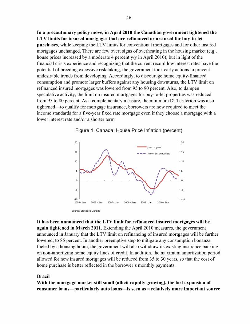
46

In a precautionary policy move, in April 2010 the Canadian government tightened the LTV limits for insured mortgages that are refinanced or are used for buy-to-let purchases, while keeping the LTV limits for conventional mortgages and for other insured mortgages unchanged. There are few overt signs of overheating in the housing market (e.g., house prices increased by a moderate 4 percent y/y in April 2010); but in light of the financial crisis experience and recognizing that the current record low interest rates have the potential of breeding excessive risk taking, the government took early actions to prevent undesirable trends from developing. Accordingly, to discourage home equity-financed consumption and promote larger buffers against any housing downturns, the LTV limit on refinanced insured mortgages was lowered from 95 to 90 percent. Also, to dampen speculative activity, the limit on insured mortgages for buy-to-let properties was reduced from 95 to 80 percent. As a complementary measure, the minimum DTI criterion was also tightened—to qualify for mortgage insurance, borrowers are now required to meet the income standards for a five-year fixed rate mortgage even if they choose a mortgage with a lower interest rate and/or a shorter term.

Figure 1. Canada: House Price Inflation (percent)

It has been announced that the LTV limit for refinanced insured mortgages will be again tightened in March 2011. Extending the April 2010 measures, the government announced in January that the LTV limit on refinancing of insured mortgages will be further lowered, to 85 percent. In another preemptive step to mitigate any consumption bonanza fueled by a housing boom, the government will also withdraw its existing insurance backing on non-amortizing home equity lines of credit. In addition, the maximum amortization period allowed for new insured mortgages will be reduced from 35 to 30 years, so that the cost of home purchase is better reflected in the borrower’s monthly payments.

Brazil With the mortgage market still small (albeit rapidly growing), the fast expansion of consumer loans—particularly auto loans—is seen as a relatively more important source

Source: Statistics Canada

-10

-5

0

5

10

15

20

-10

-5

0

5

10

15

20

2005 - Jan 2006 - Jan 2007 - Jan 2008 - Jan 2009 - Jan 2010 - Jan

year on year

3m on 3m annualized

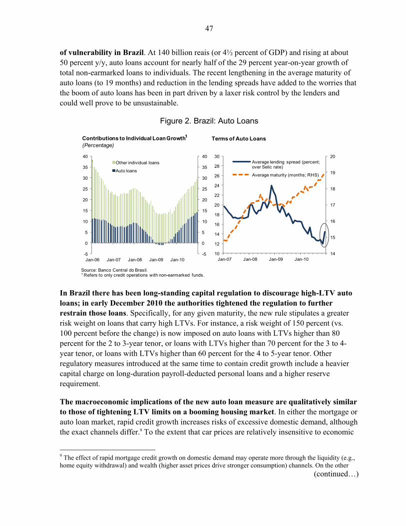
47

of vulnerability in Brazil. At 140 billion reais (or 4½ percent of GDP) and rising at about 50 percent y/y, auto loans account for nearly half of the 29 percent year-on-year growth of total non-earmarked loans to individuals. The recent lengthening in the average maturity of auto loans (to 19 months) and reduction in the lending spreads have added to the worries that the boom of auto loans has been in part driven by a laxer risk control by the lenders and could well prove to be unsustainable.

Figure 2. Brazil: Auto Loans

In Brazil there has been long-standing capital regulation to discourage high-LTV auto loans; in early December 2010 the authorities tightened the regulation to further restrain those loans. Specifically, for any given maturity, the new rule stipulates a greater risk weight on loans that carry high LTVs. For instance, a risk weight of 150 percent (vs. 100 percent before the change) is now imposed on auto loans with LTVs higher than 80 percent for the 2 to 3-year tenor, or loans with LTVs higher than 70 percent for the 3 to 4-year tenor, or loans with LTVs higher than 60 percent for the 4 to 5-year tenor. Other regulatory measures introduced at the same time to contain credit growth include a heavier capital charge on long-duration payroll-deducted personal loans and a higher reserve requirement.

The macroeconomic implications of the new auto loan measure are qualitatively similar to those of tightening LTV limits on a booming housing market. In either the mortgage or auto loan market, rapid credit growth increases risks of excessive domestic demand, although the exact channels differ.9 To the extent that car prices are relatively insensitive to economic

9 The effect of rapid mortgage credit growth on domestic demand may operate more through the liquidity (e.g., home equity withdrawal) and wealth (higher asset prices drive stronger consumption) channels. On the other

(continued…)

-5

0

5

10

15

20

25

30

35

40

-5

0

5

10

15

20

25

30

35

40

Jan-06 Jan-07 Jan-08 Jan-09 Jan-10

Other individual loans

Auto loans

Contributions to Individual LoanGrowth¹ (Percentage)

Source: Banco Central do Brasil.1 Refers to only credit operations with non-earmarked funds.

Terms of Auto Loans

14

15

16

17

18

19

20

10

12

14

16

18

20

22

24

26

28

30

Jan-07 Jan-08 Jan-09 Jan-10

Average lending spread (percent; over Selic rate)

Average maturity (months; RHS)

48

cycles, auto loan providers may be less exposed than mortgage lenders to corrections of the value of the underlying collaterals. Nevertheless, with car values depreciating quickly, providers of high-LTV and long-duration auto loans are likely to be significantly at risk from the borrowers’ repayment ability. As such, a sharp rise in credit in either the mortgage or auto loan market would similarly leave the lenders vulnerable to adverse macroeconomic shocks. Aimed to restrain the expansion of auto loans (especially the higher-risk ones), the recent measure by the Brazilian authorities could thus help lean against the domestic demand pressures and mitigate the underlying fragility of the financial sector.

In a tentative suggestion of its effectiveness, auto loan interest rates rose and domestic vehicle sales slowed immediately following the introduction of the new measure. The average auto loan interest rates increased by 2½ percentage points in the same month of the rule change, and the year-on-year change in the volume of domestic car sales was flat in January 2011, falling markedly from 24 percent in December 2010. A more complete assessment of the measure’s effectiveness, however, awaits further data, including on the volume and average maturity of auto loans.

E. Conclusion

Where the housing sector bears greater systemic consequences for the macroeconomy, LTV restriction on mortgages is more likely to be a useful macroprudential tool. In countries where the housing sector is viewed as particularly prone to boom-busts and closely tied to economic activity (due to, e.g., high share of household wealth in housing, prevalent practice of home equity withdrawal, large capital inflows to the housing sector), LTV restrictions could be a useful tool to reduce the amplitude of housing cycles and weaken their macroeconomic impacts. In many Latin American countries, the residential mortgage market is relatively shallow. And while some countries in the region already have LTV rules in place at least for the regular mortgage products (e.g., Chile, Colombia, El Salvador, Guatemala), the restrictions have not been typically adjusted along the cycles.10 Looking ahead, however, a very rapid mortgage market expansion—especially if fueled by the surge in capital inflows and/or accompanied with a fall in lending standard—would still give rise to significant risks to financial stability; by requiring lenders to hold larger collateral during the boom to buffer against the downturn, countercyclical LTV regulation could have an important prudential role to play in that context. Meanwhile, since mortgage LTV caps narrowly target the housing market, complementing this tool with wider measures to rein in financial excesses would be needed if the exuberance is widespread and beyond just the residential real estate.

hand, the effect of rapid auto loan growth on domestic demand may be more a result of a direct increase in net car purchases (as car financing becomes more abundant) and greater liquidity (car buyers have more free cash flows for non-car purchases). 10 One important exception is Chile, where the LTV requirements were lowered in 2009 for highly rated banks.

49

Moreover, LTV rules could be a useful tool even in non-housing asset markets, as highlighted by the auto loan example in Brazil. Measures to disallow or discourage high-LTV loans in other asset markets (e.g., cars, commercial real estate) work in a similar way to mortgage LTV restrictions in moderating domestic demand cycles and helping to shield the lenders from economic downturns.

The appropriate level of LTV restriction depends on the specific structure and trends of the credit market. For instance, in countries where the lenders’ financial soundness is less strong (due to, e.g., reliance on wholesale or foreign funding, low profitability) or mortgage loans are of nonrecourse nature, there may be a more compelling case for a stricter LTV limit given the lenders’ greater vulnerability to shocks. While stronger signs of overheating likely warrant a steeper LTV tightening, abrupt and aggressive policy moves might lead to an excessive correction in the asset market.11 Adjusting the LTV caps in gradual increments, on the other hand, could yield a more efficient outcome as the authorities would be better able to assess the impact of the measure and the evolving market trends before proceeding to next steps.

11 This is suggested by the recent experience in Korea, which saw a sharp reversal in the housing market dynamics following the tightening in LTV policy.

50

Annex 1. Case Study of Hong Kong SAR By way of a case study on Hong Kong SAR, this annex seeks to highlight some practical considerations relevant for the implementation of housing LTV rules. The choice of Hong Kong SAR owes to its long experience with LTV rules, and to the strong link between the housing market and the macroeconomy there.

Hong Kong SAR faces high volatility but is armed with relatively limited macroeconomic policy tools. Hong Kong SAR has a currency board arrangement and a small government, hence for macroeconomic management purposes monetary policy is absent and the fiscal tool is constrained. This provides a more prominent role to macroprudential measures. Besides its relatively small economic size and openness to international capital markets, Hong Kong SAR’s close tie to mainland China is also a key factor contributing to the economy’s volatility—on one hand, international investors’ desire to acquire financial exposures to China prompts large volumes of “proxy” investment flow to Hong Kong SAR; on the other hand, an increasing diversification of mainland Chinese’s wealth to Hong Kong SAR has helped make the territories’ housing market a speculation hotspot. Banks in Hong Kong SAR are typically highly capitalized, with low loan-to-deposit ratio. Residential mortgages represented about 27 percent of bank loans in 2010.

The LTV policy has a relatively long history in Hong Kong SAR. The restriction, at 70 percent, was first introduced in 1991 on a voluntary basis, followed by formal guidance in 1994. The denominator of the cap refers to the lower of the actual transaction price and professional surveyor’s valuation (the latter tends to be significantly less than the former during booms). The LTV cap is complemented by a DTI limit at 50–60 percent (with the upper limit applied to high earners) and guidance to banks urging against excessive property market exposures.12 The cap applies to both newly originated mortgages and refinancing, except for those refinancing cases involving negative home equity.13

Hong Kong Monetary Authority (HKMA) is responsible for the formulation and enforcement of the LTV cap. HKMA enjoys undiluted regulatory power as it is the sole prudential overseer of banks and mortgage products. While the LTV cap is not statutory, violations would result in HKMA questioning the bank’s risk management practice—a threat

12 It is “recommended” that each bank keeps mortgage loans below 40 percent of its total loans. 13 As in some other countries (e.g., Canada), borrowers are allowed to exceed the LTV cap by a limited margin if they purchase mortgage insurance. In both Hong Kong SAR and Canada, government agencies are key providers of mortgage insurance (HKMC and CMHC, respectively). In Hong Kong SAR, LTV was allowed to go up to 90 percent if accompanied by mortgage insurance (vs. 70 percent without). Standard premium on insurance provided by HKMC is about 3 percent on total loan value for mortgages with 90 percent LTV. In comparison, in Canada LTV for new mortgages is allowed to go up to 95 percent with purchase of mortgage insurance (vs. 80 percent without). Standard premium of insurance provided by CMHC is 2 percent on total loan value for mortgages with 90 percent LTV and 2.75 percent for those with 95 percent LTV. In both places, the insurance premium can be amortized over the life of the mortgage loan.

51

seen to be serious enough to make the cap essentially a rule in practice. Enforcement is done through on-site spot checks and off-site reviews. And HKMA has proved to be nimble at fine-tuning bank regulation to block loopholes—e.g., it has effectively discouraged illicit “top-ups” by moving quickly to limit the drawdown window and maturity of personal loans.14

The LTV cap has been actively managed in a countercyclical fashion. HKMA has made adjustments to the LTV rule over the years in response to housing sector developments, including a tightening of the cap in the run-up to the 1997–98 Asian crisis. More recently, in October 2009, against the backdrop of rapidly rising property prices, especially in the high-end segment, HKMA lowered the LTV cap to 60 percent for homes above HK$ million (or US$2.5 million, or about 6 times the average home price in Hong Kong SAR). In August 2010, HKMA broadened the tighter 60 percent cap to properties above HK$12 million and all buy-to-lets. As complementary measures, HKMA has also reduced the DTI limit to 50 percent for all borrowers, and required banks to grant loans only to those whose DTI would stay below 60 percent even if mortgage interest rates rise 2 percentage points.15 In November 2010, HKMA further tightened the LTV cap, to 50 percent for properties above HK$12 million and all buy-to-lets, and to 60 percent for properties between HK$8 million and HK$12 million.16

There is some early suggestive evidence that the new LTV measures might have helped slow mortgage credit growth and housing turnover, although their effects on housing prices seem less clear. Since the new measures, the weighted average of new loan LTVs has fallen—to the lowest level since at least 2001, when tracking of such data became available—probably reflecting a dropout of high LTV loans for high-end purchases (Figure A1-Chart 1). There is some suggestion that the measures might have also helped push down mortgage credit expansion and market turnover (Figure A1-Chart 2), with the targeted high-end segment particularly affected (Figure A1-Charts 3 and 4). Similarly, while the rise in average home prices has continued unabated (Figure A1-Chart 5), the relative increase in high-end home prices seems to have moderated somewhat following the new LTV rules (Chart 6). Needless to say, however, high volatility of the data and simultaneous developments of many other relevant factors suggest cautions in interpreting the outturns.17

14 Specifically, HKMA disallows personal loans to be available before the borrower closes any pending property transaction, and requires personal loans to be fully repaid within a period much shorter than the typical maturity of mortgage loans. 15 Most Hong Kong SAR homebuyers opt for variable mortgage interest rates due to their tendency to resell quickly. 16 Also in Nov 2010, the authorities imposed stricter restriction on the use of mortgage insurance to bypass the LTV cap (HKMC suspended its provision of mortgage insurance for properties above HK$6.8 million). 17 Some believe that strong demand from mainland Chinese was a key factor boosting the prices of high-end properties in Hong Kong SAR. As mainland Chinese buyers do not usually take out mortgage loans from Hong Kong SAR banks, the LTV measures might not have directly affected their demand.

52

Figure A1. Hong Kong SAR: Housing Sector Developments

52

54

56

58

60

62

64

66

68

Apr-04 Apr-05 Apr-06 Apr-07 Apr-08 Apr-09 Apr-10

High-end LTV limit tightened 1/

Chart 1. Weighted Average New Loan LTV(Percent)

Chart 2. New Mortgages Made in Secondary Market(HK$mn)

0

5,000

10,000

15,000

20,000

25,000

30,000


0

200

400

600

800

1,000

1,200

1,400

1,600


Chart 3. Property Transactions: High-end(number of cases)

0.0

0.2

0.4

0.6

0.8

1.0

1.2

1.4

1.6


Chart 4. Property Transactions: High-end divided by 2nd-tier transactions

80

90

100

110

120

130

140

150

160

170

180


Chart 5. Property Price Index (Average)

115

120

125

130

135

140

145

150


Chart 6. Property Price Index (High-end divided by average)

Sources: Hong Kong Monetary Authority and Hong Kong Mortgage Corporation.1/ Due to data limitations, high-end transactions do not fully correspond to the market segment to which the tighter LTV applies.

53

Annex 2. Recent Country Examples of LTV Restrictions

Country Dates of New Rules Latest rules

Korea Jul ’09; Oct ‘09 40–50 percent for mortgages for the capital region; looser limits for (also DTI at 40–50 percent for the capital region)

Hungary Mar ‘10 75 percent for local currency mortgages; 45–60 percent for FX mortgages

China Apr ’10; Jan ‘11 70 percent for large first homes (>90 sqm), and 40 percent for second homes

Norway Mar ‘10 90 percent for all new mortgages

Sweden Oct ‘10 85 percent for all new mortgages

Malaysia Nov ‘10 70 percent for third homes

Hong Kong SAR

Oct ’09; Aug ’10; Nov ‘10

50–60 percent for high-end purchase (>HK$8 million) and 50 percent for buy-to-lets

(also tighter DTI at 50 percent, and bank stress test required on interest rate rise)

India Dec ‘10 80 percent for higher-priced homes (>Rs 20 lakh); 90 percent for others (also higher risk weight for large mortgage loans (>Rs 75 lakh))

Brazil Dec ‘10 Higher capital charges on longer-duration, higher-LTV auto loans

Singapore Feb ’10; Aug ’10; 80 percent for buyers with no existing mortgages; 60 percent for other (also higher stamp duty for quickly resold properties)

Thailand Jan ‘11 95 percent for low-rise homes; 90 percent for most condos (<10 million bahts)

Canada Apr ’10; Mar ‘11 85 percent for refinancing of insured mortgages; 80 percent for buy-to- (also shorter maximum amortization period)

Sources: various newswires and national authorities.

54

VI. RESERVE REQUIREMENTS ON BANK LIABILITIES AS A MACROPRUDENTIAL TOOL1

A. Introduction

Emerging markets have used reserve requirements (RRs) on bank deposits and other bank liabilities as a macroprudential policy tool. Although similar in spirit to the original conception of RRs as a liquidity and credit policy tool, their use with this rationale is new. This contrasts with the long-held view that considered RRs (on deposits) a supplemental monetary policy tool for macroeconomic purposes (Goodfriend and Hargraves, 1983 or Feinman, 1993) or an integral component of a financially repressed economy (McKinnon, 1973). In that light, several countries dismantled RRs with the implementation of inflation-targeting frameworks, once short-term interest rates became the main monetary policy instrument. Nonetheless, RRs have remained part of central banks’ policy toolkit.

RRs are a regulatory tool that requires banking institutions to hold a fraction of their deposits/liabilities as liquid reserves. These are normally held at the central bank in the form of cash, or other forms, such as of government securities. When applied to deposits, the regulation usually specifies the size of the requirement according to deposit type (e.g., demand or time deposit) and its currency denomination (domestic or foreign currency). The regulation also sets the holding period relative to the reserve statement period for which the RR is computed, and whether they are remunerated or unremunerated. When they apply to new deposits only they are referred to as marginal RRs. In addition, RRs can apply to domestic or foreign (non-deposit) liabilities of bank’s balance sheets (Figure 1). Finally, RRs could be applied on assets rather than liabilities (Palley, 2004).

Figure 1. Reserve Requirements on Banks Liabilities

1 Prepared by Mercedes Garcia-Escribano, Camilo E. Tovar, and Mercedes Vera-Martin. We appreciate comments by S. Phillips, G. Terrier, R. Valdés, and C. Walker.

Reserve requirements on banks’ liabilities

Deposits

(Banks’ core funding)

In domestic currency

In foreign currency

Other liabilities

(Banks’ non-core funding)

Domestic funding

Foreign funding

55

The active management of banks’ RRs can serve different macroprudential purposes.2

First, they can serve a countercyclical role for managing the credit cycle. In the upswing, hikes in RRs may increase lending rates, slowdown credit, and limit excess leverage of borrowers in the economy, thus acting as a speed limit (see discussion below). In the downswing, they can ease liquidity constraints in the financial system, thus operating as a liquidity buffer. In this regard, RRs can serve as a flexible substitute for other macroprudential tools aiming at reducing credit dynamics. For example, they are an alternative to more distortive quantitative restrictions such as credit ceilings.

Second, RRs on foreign or domestic banks’ borrowing can help contain systemic risks by improving the funding structure of the banking system in a manner similar to what is pursued by some of the liquidity requirements proposed under Basel III (see Chapter III in this volume). They can reduce dependence on (short-term) external financing or wholesale domestic funding, reducing vulnerability of the banking sector to a rapid tightening in liquidity conditions. Peru’s active management of RRs on foreign liabilities with maturity lower than 2 years provides evidence on how RRs on banks foreign credit lines can change the composition of banks’ foreign borrowing in a juncture of large capital inflows (see annex).

Third, they can serve as a tool for credit allocation. At times of stress, an asymmetric use of RRs across instruments, sectors and financial institutions can help direct credit to ease liquidity constrains in specific sectors of the economy that threaten to have systemic implications (e.g., Brazil). In other instances is systemic risks are evident, marginal RRs can be applied to control the volume of bank credit stemming from the funding linked to the issuance of certain instruments (e.g., certificate deposits).

Fourth, RRs can play a useful complementary tool for capital requirements in countries where the valuation of assets is highly uncertain—because of a lack of liquid secondary markets, for example—as the true measurement of capital also becomes less certain.

Fifth, they have also been employed as a bank capitalization tool. In times of stress rather than lowering RRs, governments can increase their remuneration to help capitalize banks in times of stress (e.g., Korea––see below)

Finally, they can substitute some of the effects of monetary policy to achieve macroprudential goals. For example, this is evident when large capital inflows foster

2 Benefits are not necessarily additives and may exclude each other. For a general overview of the macroprudential policy discussion see IMF (2011d and 2010c).

56

rapid credit expansion and put the credit cycle at odds with monetary goals. In such instances, RRs may substitute for increases in policy interest rates (e.g., Peru).3

However, RRs are no free lunch. They have costs and may introduce distortions in the financial system. RRs limit banks’ funding and also, if remunerated below market rates, act as a tax on banks. In response, banks may raise the spread between lending and deposit rates, which may stimulate banking disintermediation, increasing nonbank financing, and giving rise to excessive risk–taking in other less regulated sectors. Also, RRs can reduce credit through the effect on bank’s funding, especially if RRs are binding (for example, for banks that do not have sufficient reserves). RRs can also generate incentives for regulatory arbitrage. In some instances, such incentives materialize in the form of a proliferation of weakly regulated “bank-like” institutions, such as off-shore banks.

Their design is complex. RRs are a blunt instrument whose calibration is not straightforward given the many variables that need to be considered. This may include deciding which banks’ liabilities (deposits or nondeposits) to target, their holding period, the RR rate itself, whether to remunerated them or not, and how to calculate and constitute the base for the regulation (e.g., lagged or contemporaneous). Also, if RRs are modified along the economic cycle, consideration needs to be given to changes in the rate and changes in the reference period. For example, changes in the marginal rate could have mostly a signaling effect; while changes in the reference period could have a higher effect on banks’ liquidity. Furthermore, marginal RRs can have adverse effects on certain institutions in the market depending on the timing in which the requirement is imposed. Finally, and no least, their level have to balance monetary and financial stability goals.

B. Theoretical Considerations

Effects of RRs on the cost and availability of credit is determined by the banking system’s market structure, the degree of financial development, and the design of RRs themselves. The market structure determines the interest rate spread and where does the burden of RRs fall on: the loan or the deposit rate. In general, changes in RRs will pass-through in whole or in part to lending interest rates in those markets where banks have some monopoly power. The extent of pass-through to lending interest rates, and hence, the amount of credit will also depend on the remuneration set for RRs. Setting aside some of these issues, it is possible to calculate the impact of RRs on interest rates using an accounting approach (Box 1).

3 RRs are also a complementary tool for foreign exchange sterilization. In periods of large capital inflows, RRs can substitute open market operations as a tool to sterilize central bank foreign exchange intervention, thus reducing their quasi-fiscal effort (especially if RRs are unremunerated).

57

The impact of RRs on credit and interest rates depends on the monetary regime in place. In a monetary aggregates regime, RRs have a direct effect on the money multiplier and, therefore on monetary aggregates and credit.4 However, in an IT regime, the effect is not obvious as the central bank stands ready to offer the liquidity necessary for the market to clear at its short-term policy rate. If central bank credit is a close bank funding substitute of deposits, higher RRs will lower deposit rates, keeping lending rates unchanged. But if this condition is not met (because it exacerbates banks’ maturity mismatches or there is uncertainty on the path of future policy short–term rates), then RRs would lower the volume of credit and drive lending interest rates up (Betancourt and Vargas, 2008). This stresses the role of imperfect substitutability across instruments and markets as a necessary condition for RRs to be effective.

RRs can be a useful instrument to bring the interbank rate close to the policy rate in situations of excessive liquidity or stress in the financial system. If banks are deposit–price takers but have some market power in lending, a hike in policy rates makes central bank credit more expensive. This forces banks to rely more on deposits, causing deposit interest rates to move up. Since the marginal cost of funds for banks increases, credit supply declines, and lending rates also increase. In this context, and as long as deposits and central bank credit are imperfect substitutes, the raise in RRs would also reinforce the transmission channel.5

Empirical evidence supporting the effectiveness of RRs as a macroprudential tool is scarce. The lack of knowledge contrasts with the wide use of this instrument to manage the

4 With financial development, the role of a money multiplier and its relevance has changed. If banks are able to securitize loans, the total quantity of loans available to the banking system is not longer less than the total amount of money in deposits, as bank-originated lending can exceed the total amount of money on deposits. 5 More analysis is required to formally evaluate the role of RRs, in particular, in a general equilibrium setting.

Box 6.1. Effect of Changes in RRs on Active Interest Rates1

The impact of RRs on active interest rates can be estimated by taking the change in the required reserved times the spread between deposit and RRs remunerated rates relative to the portion of deposits not affected by RRs. Specifically, let’s define a bank’s net margin, nm, as the return of each monetary unit lent at an active rate, ia, net of reserve requirements (1-rj), plus the return obtained by the reserve requirement itself, ir, and adjusting it by the portion of unremunerated reserve requirements, i.e. ir*(rj-rjnr), minus the passive rate. Then, the effect of changes in RRs on active rates required to maintain the net margin is:

∆∆ ∆

1 See Quispe and others, 2009.

58

credit cycle and liquidity, which suggests some effectiveness (see discussion below). An adequate empirical assessment requires constructing appropriate aggregate empirical measures beyond the deposit-specific ratios. Vargas et al. (2010), for example, construct for Colombia a tax equivalent of reserve requirements based on observed required reserve ratio; which allows considering simultaneously the effects of average and marginal reserve requirements.6 Other studies for Brazil suggest that changes in RRs on time deposits had effects on the stocks returns of the banking system. In particular, the evidence indicates that non financial corporations were the most affected by these measures, thus implying that the tax burden can be borne by bank shareholders (Carvalho and Azevedo, 2008).

C. Conclusions

RRs are a flexible and effective macroprudential tool that can address the procyclicality and, to some extent, the interconnectedness dimensions of systemic risk. RRs can address issues arising from the procyclicality of the credit cycle, building a buffer in good times that can be deployed in bad times when liquidity is required. When targeted at nondeposit liabilities it can also help improve the funding structure of the banking system, thus building a cushion in good times and diminishing the exposure of banksand therefore the extent of interconnectednessof the system in bad times. Thus, under the current juncture of excess liquidity in global markets and large capital inflows to emerging market economies (EMEs), RRs on banks can be a useful policy tool to “lean against the wind” and avoid the buildup of imbalances, in particular, associated with excessive banks’ reliance on cheap and volatile funding. Another positive aspect is that RRs also allow for targeted intervention, avoiding distortion in market or segments not affected by exuberant conditions. Finally, RRs are a useful substitute to achieve the goals of monetary policy, even in IT regimes, in particular when monetary and financial stability goals are at odds with each other.

Nonetheless, RRs have costs. Their use can induce disintermediation both through raising lending interest rates and lowering credit availability. Also, they are difficult to calibrate. Finally, as with other macroprudential tools their use needs to be complemented with other measures as it can induce risks to shift from regulated segments or sectors to unregulated ones.

Country experiences confirm that RRs have been very effective as a countercyclical tool. The reviewed experiences (see Annex 1 and 2) indicate that authorities have raised RRs during the upswing and lowered them during the downswing to ease liquidity constraintsboth before and after the global financial crisis. Moreover, to avoid distorting markets or segments not affected by over-exuberant conditions, RRs “lean-against-the-wind” in specific sectors of concern at specific junctures. Finally, so far the evidence seems to

6 Although this is a good approach for capturing liquidity changes, the approach fails to measure correctly the changes in the marginal cost of bank funds and market interest rates, and may over/underweight the role of marginal RRs.

59

suggest that RRs applied in a macroprudential do complement well monetary policy. Nonetheless, more analysis is still required, in particular in general equilibrium settings.

Going forward, policymakers may be required to revisit the calibration and scope of RRs to enhance their usefulness as a countercyclical tool. Regarding the calibration of RRs, it is important to note that exorbitant RRs rates applicable to deposits can quickly lead to disintermediation. The RR coverage should also be part of the RR design. Indeed, some EMEs are facing strong domestic growth and credit dynamics that may prove unsustainable over the medium term, despite a proactive use of RRs on deposits and/or external liabilities. One reason may be the diversion of banks’ funding from standard to more innovative sources—e.g., reliance on credit lines from non-banking financial institutions. Unlike deposits and foreign credit lines, this source of banks’ financing has not been yet subject to RRs. Expanding the coverage of RRs to loans from domestic non-monetary corporations could help limit excessive reliance of banks on these as source of funding, and reduce network risks within the domestic financial system.

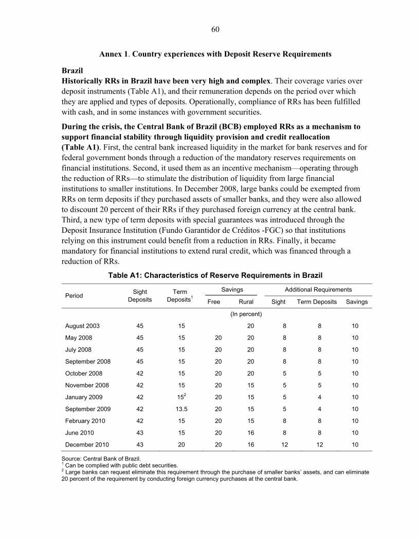
60

Annex 1. Country experiences with Deposit Reserve Requirements

Brazil Historically RRs in Brazil have been very high and complex. Their coverage varies over deposit instruments (Table A1), and their remuneration depends on the period over which they are applied and types of deposits. Operationally, compliance of RRs has been fulfilled with cash, and in some instances with government securities.

During the crisis, the Central Bank of Brazil (BCB) employed RRs as a mechanism to support financial stability through liquidity provision and credit reallocation (Table A1). First, the central bank increased liquidity in the market for bank reserves and for federal government bonds through a reduction of the mandatory reserves requirements on financial institutions. Second, it used them as an incentive mechanism—operating through the reduction of RRs—to stimulate the distribution of liquidity from large financial institutions to smaller institutions. In December 2008, large banks could be exempted from RRs on term deposits if they purchased assets of smaller banks, and they were also allowed to discount 20 percent of their RRs if they purchased foreign currency at the central bank. Third, a new type of term deposits with special guarantees was introduced through the Deposit Insurance Institution (Fundo Garantidor de Créditos -FGC) so that institutions relying on this instrument could benefit from a reduction in RRs. Finally, it became mandatory for financial institutions to extend rural credit, which was financed through a reduction of RRs.

Table A1: Characteristics of Reserve Requirements in Brazil

Period Sight

Deposits Term

Deposits1

Savings Additional Requirements

Free Rural Sight Term Deposits Savings

(In percent)

August 2003 45 15 20 8 8 10

May 2008 45 15 20 20 8 8 10

July 2008 45 15 20 20 8 8 10

September 2008 45 15 20 20 8 8 10

October 2008 42 15 20 20 5 5 10

November 2008 42 15 20 15 5 5 10

January 2009 42 152 20 15 5 4 10

September 2009 42 13.5 20 15 5 4 10

February 2010 42 15 20 15 8 8 10

June 2010 43 15 20 16 8 8 10

December 2010 43 20 20 16 12 12 10

Source: Central Bank of Brazil. 1 Can be complied with public debt securities. 2 Large banks can request eliminate this requirement through the purchase of smaller banks’ assets, and can eliminate 20 percent of the requirement by conducting foreign currency purchases at the central bank.

61

Lately, RRs have served as a tool for managing the boom. Recently, RRs on deposits were increased beyond levels prevalent prior to Lehman’s episode. Furthermore, in January 2011, the BCB introduced new RRs that seek to limit the short dollar position of banks in the spot market (see companion note “Limiting net foreign exchange positions” by Fernández-Valdovinos and Walker). This measure also aims at discouraging carry trade operations and moderate short-term appreciation pressures on the real.

Colombia The Central Bank of Colombia (Banco de la República, BdR) has employed RRs over the cycle to slowdown credit growth in the context of large capital inflows. BdR introduced marginal RRs on domestic deposits (CDs, checking and savings accounts) in May 2007 to contain the rapid credit growth in the economy and stop the quality deterioration of new vintages of loans (Table A2). Credit dynamics seemed to be driven by a supply shift. This prompted measures to curtail the excessive leverage of the private sector and control credit risk of the financial system. RRs on domestic deposits were complemented with RRs on foreign indebtedness (see accompanying note on “RRs on capital inflows”), and higher loan provisioning requirements.

During the global crisis, RRs served a preventive role for liquidity provision. RRs were lowered and marginal reserve requirements were eliminated in the third quarter of 2008 when the economy began to show signs of a slowdown and the global business environment became very uncertain. These adjustments were complemented with further easing during 2009 (Table A2). Overall, RRs have varied over cycle, and authorities have applied them over different instruments. In some instances, marginal RRs have also been employed (Table 2).7

Econometric evidence suggests that RRs operate by making financial intermediation more expensive and that they have been a relevant determinant of business loan interest rates. Furthermore, that they have strengthened the interest rate pass-through from policy to deposit rates and to lending rates. Specifically, evidence for the period 2002–09 indicates a positive long run relationship between policy rates and market rates-except for mortgage rates. The evidence also suggests that marginal RRs on CDs have a significant impact in the longer term and average CD rates, even though CDs have zero RRs. This result may imply that RRs induce a shift in the composition of the deposit structure (Vargas et al, 2010).

7 The range of deposits subject to RRs is includes checking accounts, simple accounts, savings, real savings, special savings, centralized accounts, different transfer agreements on repo operations, some term deposits, some bonds, certificate deposits, and other more specific items.

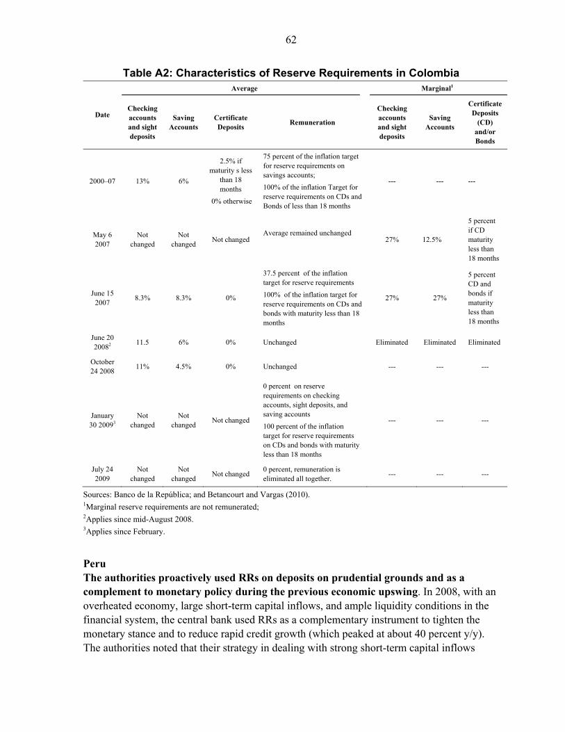
62

Table A2: Characteristics of Reserve Requirements in Colombia

Sources: Banco de la República; and Betancourt and Vargas (2010). 1Marginal reserve requirements are not remunerated; 2Applies since mid-August 2008. 3Applies since February.

Peru The authorities proactively used RRs on deposits on prudential grounds and as a complement to monetary policy during the previous economic upswing. In 2008, with an overheated economy, large short-term capital inflows, and ample liquidity conditions in the financial system, the central bank used RRs as a complementary instrument to tighten the monetary stance and to reduce rapid credit growth (which peaked at about 40 percent y/y). The authorities noted that their strategy in dealing with strong short-term capital inflows

Date

Average Marginal1

Checking accounts and sight deposits

Saving Accounts

Certificate Deposits

Remuneration

Checking accounts and sight deposits

Saving Accounts

Certificate Deposits

(CD) and/or Bonds

2000–07 13% 6%

2.5% if maturity s less

than 18 months

0% otherwise

75 percent of the inflation target for reserve requirements on savings accounts;

100% of the inflation Target for reserve requirements on CDs and Bonds of less than 18 months

--- --- ---

May 6 2007

Not changed

Not changed

Not changed

Average remained unchanged 27% 12.5%

5 percent if CD maturity less than 18 months

June 15 2007

8.3% 8.3% 0%

37.5 percent of the inflation target for reserve requirements

100% of the inflation target for reserve requirements on CDs and bonds with maturity less than 18 months

27% 27%

5 percent CD and bonds if maturity less than 18 months

June 20 20082

11.5 6% 0% Unchanged Eliminated Eliminated Eliminated

October 24 2008

11% 4.5% 0% Unchanged --- --- ---

January 30 20093

Not changed

Not changed

Not changed

0 percent on reserve requirements on checking accounts, sight deposits, and saving accounts

100 percent of the inflation target for reserve requirements on CDs and bonds with maturity less than 18 months

--- --- ---

July 24 2009

Not changed

Not changed

Not changed 0 percent, remuneration is eliminated all together.

--- --- ---

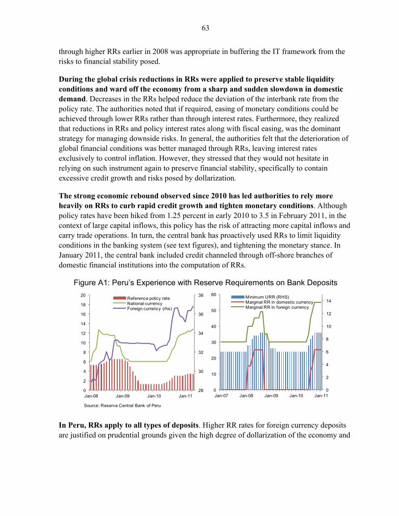
63

through higher RRs earlier in 2008 was appropriate in buffering the IT framework from the risks to financial stability posed.

During the global crisis reductions in RRs were applied to preserve stable liquidity conditions and ward off the economy from a sharp and sudden slowdown in domestic demand. Decreases in the RRs helped reduce the deviation of the interbank rate from the policy rate. The authorities noted that if required, easing of monetary conditions could be achieved through lower RRs rather than through interest rates. Furthermore, they realized that reductions in RRs and policy interest rates along with fiscal easing, was the dominant strategy for managing downside risks. In general, the authorities felt that the deterioration of global financial conditions was better managed through RRs, leaving interest rates exclusively to control inflation. However, they stressed that they would not hesitate in relying on such instrument again to preserve financial stability, specifically to contain excessive credit growth and risks posed by dollarization.

The strong economic rebound observed since 2010 has led authorities to rely more heavily on RRs to curb rapid credit growth and tighten monetary conditions. Although policy rates have been hiked from 1.25 percent in early 2010 to 3.5 in February 2011, in the context of large capital inflows, this policy has the risk of attracting more capital inflows and carry trade operations. In turn, the central bank has proactively used RRs to limit liquidity conditions in the banking system (see text figures), and tightening the monetary stance. In January 2011, the central bank included credit channeled through off-shore branches of domestic financial institutions into the computation of RRs.

Figure A1: Peru’s Experience with Reserve Requirements on Bank Deposits

In Peru, RRs apply to all types of deposits. Higher RR rates for foreign currency deposits are justified on prudential grounds given the high degree of dollarization of the economy and

28

30

32

34

36

38

0

2

4

6

8

10

12

14

16

18

20

Jan-08 Jan-09 Jan-10 Jan-11

Reference policy rateNational currencyForeign currency (rhs)

0

2

4

6

8

10

12

14

0

10

20

30

40

50

60

Jan-07 Jan-08 Jan-09 Jan-10 Jan-11

Minimum URR (RHS)Marginal RR in domestic currencyMarginal RR in foreign currency

Source: Reserve Central Bank of Peru

64

the central bank’s inability to print foreign currency in times of liquidity shortages.8 To calculate RRs, financial institutions first identify the total liabilities subject to RRs, and then compute the daily average for the month. Legal RRs rate apply to this daily average. For the marginal rate, the average in the month is compared to the one during the reference period (currently December 2010). The marginal requirement is then applied to the excess, and remuneration is depicted in Table A3. The sum of these two components is the total RR, and the implicit rate is the average rate for the RRs.9 Banks are allowed to have RRs above or below the minimum required. In case of a shortage, the institution is fined, and if it is recurrent, the institution can be taken into a special monitoring regime of the Superintendence.

Table A3. Peru: Deposit Reserve Requirements, February 2011

Legal rate Marginal Rate Effective Rate Remuneration

(unremunerated)

In domestic currency 9 251 12.3

Overnight rate-100 bps

In foreign currency 9 55

35.2 0.6*Libor (1 month)

Source: BCRP. 1 For residents. The marginal rate for nonresidents is 120 percent.

Peruvian authorities report that a 1 percentage point increase in RRs rate has an equivalent effect over the output gap as a 25 bps increase in the policy rate.10 Also, a 1 percentage point increase in the RR raises one-year interest rates by 0.24 percentage point and decrease passive interest rates.

China During 2010, the Chinese authorities’ raised RRs amid growing concerns about accelerating inflation and rapid money and credit growth. Domestic demand has been boosted by commercial banks’ frontloading of lending since early 2010, and continued strength in FX

8 In some instances, local currency–denominated deposits are exonerated, for deposits of S/ 50 million or 5.6 percent of the total liabilities subject to RRs, whichever smaller. 9 As of September 2010, this average rate was 9.1 percent for domestic currency deposits and 36.9 percent for foreign currency deposits. As of October 2010, the stock of domestic-currency RR amounted to S/. 6.9 billion (1.6 percent of 2010 GDP). Notice also that there is no substitutability among assets denominated in either currency. 10 This result is calculated using a framework similar to that described in footnote 10, and is based on an active average rate of 19.5 percent, a reserve requirement of 6 percent, and no RR remuneration.

65

inflows provides additional liquidity to the real economy.11 Against this background a consensus has emerged on the need to tighten policy further. Given that large scale changes in market-based tools (e.g., interest rate and exchange rate) would be needed to cool down the economy are unlikely, most of the heavy lifting has fallen on administrative measures. RRs are considered a better alternative to price controls, which tend to send distorted signals.

Hikes of RRs aim at signaling the central bank’s tightening policy stance. The central bank hiked RRs 100 bps since January 2011 to 20 percent for large banks and 18 percent for small banks, representing the fourth tightening in two months. This was estimated to be equivalent to a reduction of Y360 billion in deposits (0.9 percent of 2010 GDP). Goldman Sachs estimates that the RR ratio is not binding on commercial banks’ ability to lend as the excess reserve ratio is estimated to be between 1.5 percent and 2 percent.12

Figure A2: China’s Management of Reserve Requirements

Turkey In December 2010, the Central Bank of Turkey (CBT) increased and broadened the scope of domestic currency RRs, with the aim of increasing the cost of short-term funding for domestic banks and limiting domestic credit expansion. However, reports indicate that timid RRs hikes will be insufficient to rebalance the economy, in the absence of a strong counter-cyclical fiscal policy response and given the easy domestic financial conditions, which are reinforced by low nominal rates and a weaker exchange rate.

11 External demand has also been accelerating as well, adding fuel to aggregate demand pressures; and short-term food prices have started to rebound amid adverse weather conditions. 12 Going forward, for the year as a whole, analysts are expecting at least 200 bps in RR hikes owing to concerns about surging FX inflows, price pressures, and bank lending. Consecutive RR hikes will likely make it more difficult for them to keep lending at a fast pace.

14

15

16

17

18

19

20

14

15

16

17

18

19

20

Jan- 08 Jul-08 Jan-09 Jul-09 Jan-10 Jul-10 Jan-11

Source: People's Bank of China

66

The central bank also lowered policy rates with higher RRs. To enhance financial stability, the scope of the RRs was widened to include some repo operations,13 and to encourage long term funding RRs ratios were set to differ across domestic currency deposits with different maturities. Specifically, RR ratios––previously set at 6 percent—were set as follows: (i) 8 percent for demand deposits, notice deposits, private current accounts, deposits accounts up to 1-month maturity and liabilities other than deposits accounts; (ii) 7 percent for deposits accounts up to 3 and 6-month maturity; (iii) 6 percent for deposits accounts up to 1-year maturity; (iv) 5 percent for deposits accounts with 1-year and longer maturity and cumulative deposits accounts. To ensure the effectiveness of the policy, interest rates on demand deposits were capped at 0.25 percent annually. The new measures are expected to reduce market liquidity by approximately TL7.6 billion and US$200 million (0.7 percent of 2010 GDP, 2.3 percent of 2009 total claims to the private sector).

Korea The Bank of Korea (BoK) used RRs during the crisis as a tool for capitalizing the banking system and therefore boosting its lending capacity. Thus their use had a different goal than in Latin America. Specifically, in December 2008, the BoK increased the banking system capital adequacy ratios by paying a one-off interest of W500.2 billion on RRs (0.05 percent of GDP). The advantage of this measure, rather than simply lowering banks’ RRs, was that it immediately improved bank balance sheets.

13 The RR base was expanded to include funds received by banks through repurchase agreement (repo) transactions from abroad and domestic customers, except for those funds received from repo transactions with the Central Bank and those among domestic banks.

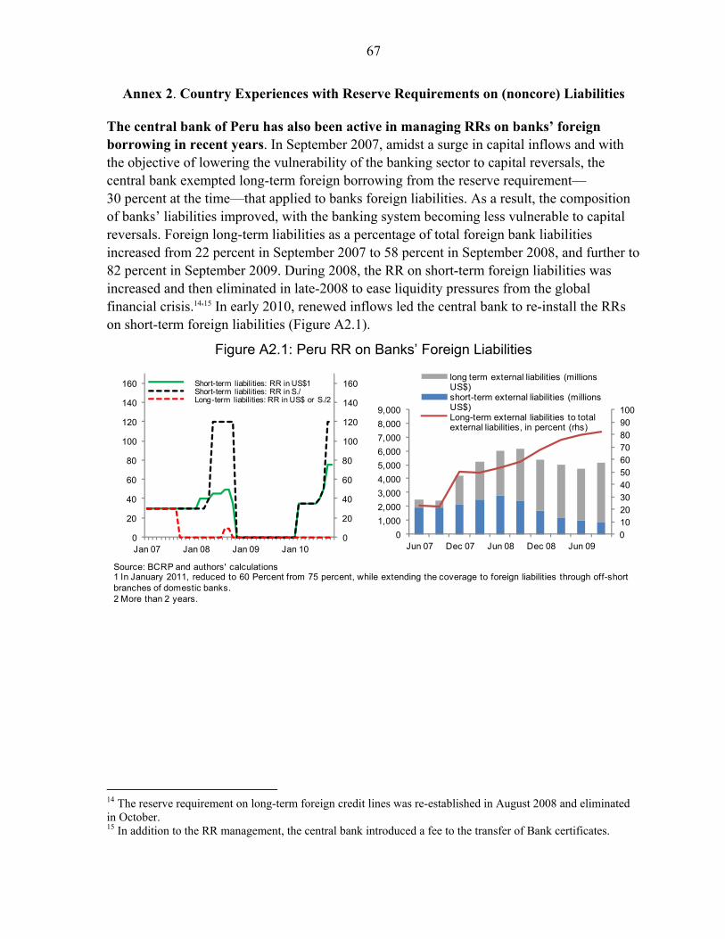
67

Annex 2. Country Experiences with Reserve Requirements on (noncore) Liabilities

The central bank of Peru has also been active in managing RRs on banks’ foreign borrowing in recent years. In September 2007, amidst a surge in capital inflows and with the objective of lowering the vulnerability of the banking sector to capital reversals, the central bank exempted long-term foreign borrowing from the reserve requirement—30 percent at the time—that applied to banks foreign liabilities. As a result, the composition of banks’ liabilities improved, with the banking system becoming less vulnerable to capital reversals. Foreign long-term liabilities as a percentage of total foreign bank liabilities increased from 22 percent in September 2007 to 58 percent in September 2008, and further to 82 percent in September 2009. During 2008, the RR on short-term foreign liabilities was increased and then eliminated in late-2008 to ease liquidity pressures from the global financial crisis.14,15 In early 2010, renewed inflows led the central bank to re-install the RRs on short-term foreign liabilities (Figure A2.1).

Figure A2.1: Peru RR on Banks’ Foreign Liabilities

14 The reserve requirement on long-term foreign credit lines was re-established in August 2008 and eliminated in October. 15 In addition to the RR management, the central bank introduced a fee to the transfer of Bank certificates.

0

20

40

60

80

100

120

140

160

0

20

40

60

80

100

120

140

160

Jan 07 Jan 08 Jan 09 Jan 10

Short-term liabilities: RR in US$1Short-term liabilities: RR in S./ Long-term liabilities: RR in US$ or S./2

Source: BCRP and authors' calculations1 In January 2011, reduced to 60 Percent from 75 percent, while extending the coverage to foreign liabilities through off-short branches of domestic banks.2 More than 2 years.

0

10203040

50607080

90100

0

1,000

2,000

3,000

4,000

5,000

6,000

7,000

8,000

9,000

Jun 07 Dec 07 Jun 08 Dec 08 Jun 09

long term external liabilities (millions US$)short-term external liabilities (millions US$)Long-term external liabilities to total external liabilities, in percent (rhs)

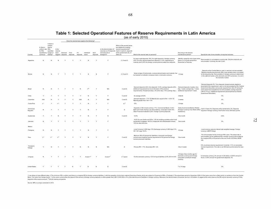
68

Table 1: Selected Operational Features of Reserve Requirements in Latin America (as of early 2010)

Demand deposits

Time deposits

FX deposits

Interbank loans

Govt deposits

Argentina N N N Y Y Y N Y F C, D and OFor peso sight deposits,19%; For sight deposits in foreign currency, 20%; For peso denominated time deposits, 0-14%, depending on maturity; and 0-20% for foreign currency denominated time deposits.

Monthly, except for end of year when there is a 3-month period from December to February

Remuneration is not related to a policy rate. Only time deposits are remunerated. Currently, the rate is zero.

Bolivia N N Y Y Y Y N N F C, D and OVaries by type of instruments, currency denomination and maturity. Can be lowered is institution increases loans in domestic currency.

14 days

Deposits at the Central Bank or cash in vault are not remunerated. Statutory liquidity requirements (RAL) have variable return not related to the key policy rate. Remuneration in foreign currency is determined in the external market, while domestic and UFV currencies, it is set in

the domestic market.

Brazil N N Y Y Y N Y10 Y N/A C and D Demand deposits 42%; time deposits 13.5%; savings deposits 20%; additional requirement (a mix on the basis of the previous requirements): 5%(demand dep.); 4% (time dep.) 10% (savings dep.)

Demand deposits 2 weeks, time dep. 1 week, savings dep. 1 week, additional requirement 1 week.

Demand deposits 0%; Time deposits (several assets eligible to accomplish this requirement: cash is not remunerated by CB, Federal Government Securities and assets acquired from other IF during the crisis period are accepted but not remunerated), savings deposits (TR+6.17% py ), additional requirement (accomplished by Federal Government Securities).

Chile Y Y Y Y Y Y N Y F C and D An average of 6.6% A Month 0%

Colombia N/A N Y Y Y N/A N Y N/A C and D Demand deposits = 11% TD Maturity less equal to18m = 4,5% TD Maturity greater than 18m = 0%

2 weeks 0%

Costa Rica Y 1 Y Y 4 Y Y Y N Y F D 9/ 15% 15 days 0%

Dominican Republic

N Y Y Y Y Y N Y F D Deposits in CB in local currency: 17% -Commercial Banks 12.5% -Bank and Credit, Saving Loan Associations, Corporate Credit 10% -Other Financial Institutions 20% -Foreign Currency Deposits

Daily (Commercial Banks) Weekly (Foreign Currency) Two Week (Other Institutions)

Cash in Vault, 0%; Deposits at the central bank, 0%; Deposits required in foreign currency, Fed Funds minus 200 basic points.

Guatemala Y Y N Y Y Y N Y N C and D 14.6% One month 0.6%

Jamaica N Y Y Y Y Y Y Y F 14.0% for com banks and OFIs; 1.0% for building societies which hold residential mortgages =40.0% of deposits and withdrawable shares; 14% for other bld socs.

One month 0%

Mexico

Paraguay N N Y Y Y Y N Y F Local Currency: 0-360 days 15% Exchange currency: 0-360 days 21% , 361- 541 days 16,5%.

30 days Local currency: passive interest rate weighted average. Foreign currency: LIBOR 30days

Peru Y 2 Y 3 Y 5 Y Y Y N Y F C and D Minimum RR of 6 percent for liabilities in domestic and foreign currency and marginal reserve requirement of 30 percent for foreign currency domestic liabilities.

One month

The remuneration for the minimum RR is zero. The actual rate of remuneration for the additional RR in foreign currency (associated to the marginal RR) is 60 percent of the one month US Dollar LIBOR rate.

Trinidad & Tobago

Y N Y Y Y N N N N/A D Primary RR = 17%. Secondary RR = 2% One (1) weekO% on primary reserve requirement. Currently, 1.5 % on secondary reserve requirement. This rate is set 350 basis points below the repo rate.

Uruguay N Y Y Y Y Y N and Y 6 Y D and F 7 C 8 and D For the domestic currency: 12% for liquid liabilities (l) 9% 29<l<l<l181

30 days of two months ago for domestic currency and 30 days computed currently for foreign currency

In domestic currency, 2% annual; In US dollars, 0.025% annual; In Euros, 0.20% annual; For government deposits, 0%.

United States Y Y Y Y N Y N N D C and D 7 or 14 days 0%

Source: IMF on surveys conducted in 2010.

How long is the reserve maintenance period? Specify the rate of remuneration of required reserves.

1 Law allows to have different rates; 2 The minimum RR is uniform and there is a marginal RR for foreign currency liabilities; 3 with the exception of short term external financing of banks which are subject to 35 percent of RRs; 4 Fortnight; 5 The actual base period is November 2008; 6 if the loans come from a Bank which is resident or from the Central Bank, Y for loans from foreign banks. 7 In the same currency than the deposit if the amount of foreign currency deposits is either greater than U$S 10.000.000 or 5% of the total amount of liabilities in foreign currency. Otherwise, the denomination of reserves can be in US dollars; 8 Lagged at the same base as the RR only for domestic currency; 9 Only

deposits at the reserve account; 10 Only for leasing companies

Which of the assets below are eligible for meeting reserve requirements? Cash in vault (C), deposits at the central bank (D), or other (O)

Does the reserve base apply to the following?

Country

Is there a uniform rate for RRs specified by currency?

Is there a uniform rate for RRs specified by type of liability? What is the reserve ratio (in percent)?

Is the reserve base lagged?

Is the denomination of reserves on FX deposits domestic (D) or foreign(F)?

72

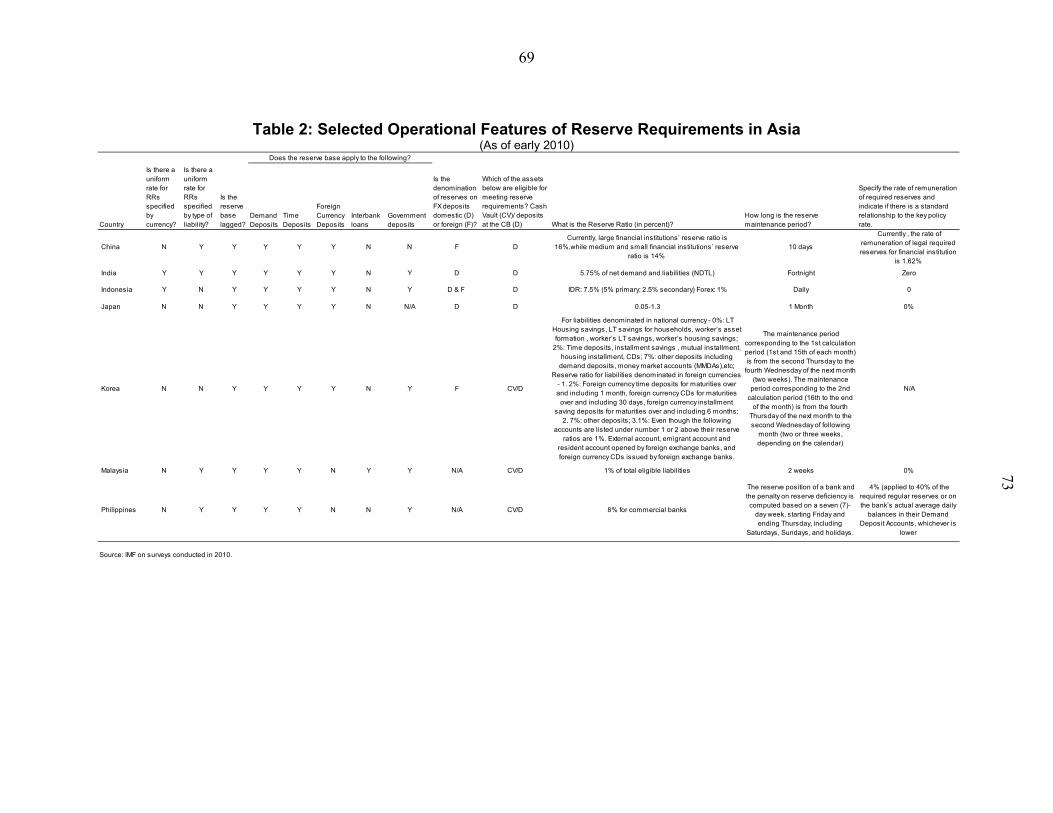
69

Table 2: Selected Operational Features of Reserve Requirements in Asia (As of early 2010)

Demand Deposits

Time Deposits

Foreign Currency Deposits

Interbank loans

Government deposits

China N Y Y Y Y Y N N F D Currently, large financial institutions’ reserve ratio is

16%,while medium and small financial institutions’ reserve ratio is 14%

10 days

Currently , the rate of remuneration of legal required reserves for financial institution

is 1.62%

India Y Y Y Y Y Y N Y D D 5.75% of net demand and liabilities (NDTL) Fortnight Zero

Indonesia Y N Y Y Y Y N Y D & F D IDR: 7.5% (5% primary; 2.5% secondary) Forex: 1% Daily 0

Japan N N Y Y Y Y N N/A D D 0.05-1.3 1 Month 0%

Korea N N Y Y Y Y N Y F CV/D

For liabilities denominated in national currency - 0%: LT Housing savings, LT savings for households, worker’s asset formation , worker’s LT savings, worker’s housing savings;

2%: Time deposits, installment savings , mutual installment, housing installment, CDs; 7%: other deposits including demand deposits, money market accounts (MMDAs),etc;

Reserve ratio for liabilities denominated in foreign currencies - 1. 2%: Foreign currency time deposits for maturities over and including 1 month, foreign currency CDs for maturities

over and including 30 days, foreign currency installment saving deposits for maturities over and including 6 months;

2. 7%: other deposits; 3.1%: Even though the following accounts are listed under number 1 or 2 above their reserve

ratios are 1%. External account, emigrant account and resident account opened by foreign exchange banks, and foreign currency CDs issued by foreign exchange banks.

The maintenance period corresponding to the 1st calculation period (1st and 15th of each month) is from the second Thursday to the fourth Wednesday of the next month

(two weeks). The maintenance period corresponding to the 2nd

calculation period (16th to the end of the month) is from the fourth

Thursday of the next month to the second Wednesday of following

month (two or three weeks, depending on the calendar)

N/A

Malaysia N Y Y Y Y N Y Y N/A CV/D 1% of total eligible liabilities 2 weeks 0%

Philippines N Y Y Y Y N N Y N/A CV/D 8% for commercial banks

The reserve position of a bank and the penalty on reserve deficiency is computed based on a seven (7)-

day week, starting Friday and ending Thursday, including

Saturdays, Sundays, and holidays.

4% (applied to 40% of the required regular reserves or on the bank’s actual average daily

balances in their Demand Deposit Accounts, whichever is

lower

Source: IMF on surveys conducted in 2010.

Country


Is there a uniform rate for RRs specified by type of liability?



Is the denomination of reserves on FX deposits domestic (D) or foreign (F)? What is the Reserve Ratio (in percent)?

How long is the reserve maintenance period?

Specify the rate of remuneration of required reserves and indicate if there is a standard relationship to the key policy rate.

Which of the assets below are eligible for meeting reserve requirements? Cash Vault (CV)/ deposits at the CB (D)

73

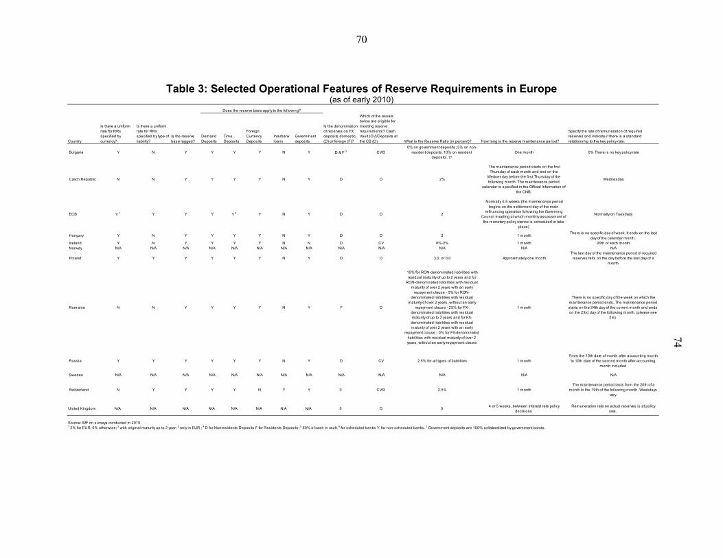
70

Table 3: Selected Operational Features of Reserve Requirements in Europe (as of early 2010)

Demand Deposits

Time Deposits

Foreign Currency Deposits

Interbank loans

Government deposits

Which of the assets below are eligible for meeting reserve requirements? Cash Vault (CV)/Deposits at the CB (D)

Bulgaria Y N Y Y Y Y N Y D & F 3 CV/D 0% on government deposits; 5% on non-

resident deposits; 10% on resident deposits. 7/

One month 0% There is no key policy rate

Czech Republic N N Y Y Y Y N Y D D 2%

The maintenance period starts on the first Thursday of each month and end on the

Wednesday before the first Thursday of the following month. The maintenance period

calendar is specified in the Official Information of the CNB.

Wednesday

ECB Y 1 Y Y Y Y 2 Y N Y D D 2

Normally 4-5 weeks (the maintenance period begins on the settlement day of the main

refinancing operation following the Governing Council meeting at which monthly assessment of the monetary policy stance is scheduled to take

place)

Normally on Tuesdays

Hungary Y N Y Y Y Y N Y D D 2 1 month There is no specific day of week. It ends on the last

day of the calendar month. Iceland Y N Y Y Y Y N N D CV 0%-2% 1 month 20th of each month Norway N/A N/A N/A N/A N/A N/A N/A N/A N/A N/A N/A N/A N/A

Poland Y Y Y Y Y Y N Y D D 3,0. or 0,0 Approximately one month The last day of the maintenance period of required

reserves falls on the day before the last day of a month

Romania N N Y Y Y Y N Y F D

15% for RON-denominated liabilities with residual maturity of up to 2 years and for

RON-denominated liabilities with residual maturity of over 2 years with an early

repayment clause - 0% for RON-denominated liabilities with residual

maturity of over 2 years, without an early repayment clause - 25% for FX-

denominated liabilities with residual maturity of up to 2 years and for FX-denominated liabilities with residual maturity of over 2 years with an early

repayment clause - 0% for FX-denominated liabilities with residual maturity of over 2 years, without an early repayment clause

1 month

There is no specific day of the week on which the maintenance period ends. The maintenance period starts on the 24th day of the current month and ends on the 23rd day of the following month. (please see

2.6).

Russia Y Y Y Y Y Y N Y D CV 2.5% for all types of liabilities 1 monthFrom the 10th date of month after accounting month to 10th date of the second month after accounting

month included

Sweden N/A N/A N/A N/A N/A N/A N/A N/A N/A N/A N/A N/A N/A

Switzerland N Y Y Y Y N Y Y 0 CV/D 2.5% 1 month The maintenance period lasts from the 20th of a

month to the 19th of the following month. Weekdays vary.

United Kingdom N/A N/A N/A N/A N/A N/A N/A N/A 0 D 0 4 or 5 weeks, between interest rate policy

decisions Remuneration rate on actual reserves is at policy

rate.

Source: IMF on surveys conducted in 2010.1 2% for EUR, 0% otherwise; 2 with original maturity up to 2 year; 3 only in EUR ; 4 D for Nonresidents Deposits F for Residents Deposits; 5 50% of cash in vault; 6 for scheduled banks Y, for non-scheduled banks. 7 Government deposits are 100% collateralized by government bonds.

What is the Reserve Ratio (in percent)?Country


Is there a uniform rate for RRs specified by type of liability?



Is the denomination of reserves on FX deposits domestic (D) or foreign (F)? How long is the reserve maintenance period?

Specify the rate of remuneration of required reserves and indicate if there is a standard relationship to the key policy rate.

74

71

VII. MACROPRUDENTIAL INSTRUMENTS TO MANAGE FOREIGN-EXCHANGE CREDIT RISK1

A. Motivation

Foreign-exchange (FX) credit risk can pose significant systemic risk to the financial system and the economy as a whole. FX credit risk is the risk faced by financial institutions associated with lending to unhedged borrowers that carry currency mismatches in their balance sheets. Experience in EMs—more recently in Europe—has shown that currency mismatch has been a prime vehicle for agents to take on credit risk, and has resulted in large exposures to systemic risk for the economy as a whole. In an environment of economic bonanza and rapid credit growth, banks may not be appropriately pricing or provisioning for the indirect exposures to FX risk. Banks’ currency risk from FX liabilities can be largely passed on to borrowers via FX loans; which could backfire if a large FX depreciation were to increase the debt burden of borrowers and lead to defaults.2

Although currency mismatches may be limited in the banking sector balance sheet; FX lending pose important credit risks that are difficult to assess. FX credit risks are very difficult to calibrate, and for financial institutions to internalize. The credit risk are associated not only with the direct exposure (when the bank extends FX-denominated credit to un-hedged borrowers), but also with an indirect exposure (the bank extends domestic-currency lending to a borrower who is already exposed to FX risks). Lack of information about the corporates and households’ structure of debt obligations (currency and maturity) and financial exposures, including to derivatives, hinders also the effective assessment of FX credit risk. The most vulnerable sector may be the household sector; although the presence of FX deposits in dollarized economies may mitigate this risk to a certain extent.

Countries have implemented prudential measures to make financial institutions internalize FX credit risks associated with lending to un-hedged borrowing. Measures to limit FX lending in Emerging Europe before the global financial crisis through reserve requirements on FX liabilities and limits to FX exposure to banks or limits on FX lending as a percent of capital were not very effective as they were circumvented under easy external financing conditions. However, those measures were not specifically designed to deal with FX credit risks; as banks did not internalize the risks of lending in foreign exchange to un-hedged borrowers. Recent measures focus on additional provisioning and capital requirements; but it is too early to assess their effectiveness. As a first step, authorities may request financial institutions to establish a system to identify and monitor FX risks, as well as internal procedures to manage such risks, and take corrective measures as required. But there

1 Prepared by Mercedes Vera Martin. The note has benefited from comments by C. Fernandez, M. Garcia-Escribano, and C. Tovar. 2 For a discussion on measures to limit FX positions in banks’ balance sheets, see accompanying note “Limiting Foreign Exchange Positions to Contain Systemic Risk,” prepared by C. Fernández-Valdovinos and Chris Walker (WHD).

72

is also a need to enhance supervision on this front, to ensure that financial institutions are accordingly evaluating the FX credit risks.

B. Instruments and Potential Benefits

Measures to limit FX credit risk enhance financial stability by ultimately reducing potential losses associated with large currency depreciation at time of financial stress. The measures help banks internalize FX risks associated to lending to un-hedged borrowers. Country experiences showed a focus on direct exposures; with no attempt to incorporate indirect credit risks (Annex I). The measures could also serve as a counter-cyclical tool if they help curb FX lending (at least) in the short run. The measures make FX lending more costly for financial institutions, and can act as a deterrent to extend FX loans. Regarding quantitative measures, debt to income limits on borrowers may be more effective than bank credit limits as a percent of capital. In Romania; limits on domestic FX lending as a percent of capital had some temporary effects, but effects faded away as financial institutions found ways to raise capital at times of easy external financial conditions. Significant risks to financial disintermediation also rose as households and corporate search for alternative sources of funding. Limits on debt-to-income for individual loans extended in foreign currency could be more effective, and sometimes result in an effective banning of FX lending through specific instruments (i.e. mortgages). These limits are more stringent that those impose for lending extended in domestic currency, which somehow assess impairments on borrowers’ ability to service their debt under an implicit level of depreciation (see the case of Uruguay). Additional capital or provisioning requirements seem more adequate to account for the FX credit risks. While the difference between provisioning and capital requirements may not be so clear, in line with general wisdom, one could consider a preference for provisioning to account for expected losses derived from FX credit risks—for example, by taking into account the identified direct FX exposure extended through credit. Additional capital requirements could then account for unexpected losses; from unidentified FX credit risk because it is unknown the extent of FX exposure to specific clients, or because of indirect exposures. Two countries (Peru and Uruguay) explicitly request additional capital requirements on FX credit risk. Peru establishes a capital add-on taking into account the FX exposure; while Uruguay establishes a higher risk weight for loans extended in foreign currency to un-hedged borrowers. The latter may be a more transparent way to establish additional capital requirements, because of the difficulties in calibrating the FX exposure. To be effective, measures need to result in a higher cost associated to FX lending to financial institutions.

As a first step, country authorities need to do more to compile detailed information about the financing structure of the corporate and household sectors in a systematic way, with emphasis on FX mismatches and exposure to complex financial instruments like

73

derivatives. To properly internalize FX credit risks, information is required on FX position, FX sales and percentage of short-term liabilities in foreign currency from the borrowers, which may prove challenging. Lack of information about the corporates and households’ structure of debt obligations (currency and maturity) and financial exposures, including to derivatives, hinders also the effective assessment of FX credit risk; and exacerbated the impact of the global financial crisis. Limitations on the latter were evidenced in Brazil and Mexico in 2008, when large corporate losses materialized due to FX operations in the FX derivative market (see Annex I). In parallel, measures to encourage the adequate use of FX hedging among the household and corporate sectors would be welcome.

And enhanced supervision is required. Supervisory authorities need to fully understand/monitor how financial institutions identify FX credit risks; and stand ready to adapt regulation. In this regard, some homogenous framework across the financial system would be welcome, so that there is some benchmarking in the evaluation of FX credit risks across financial institutions risk evaluation systems.

74

Annex 1. Country Experiences in Managing FX Credit Risk This annex surveys the experiences with specific prudential measures managing FX credit risks. Measure have not been widely use despite being a considerable threat to financial stability. The main challenge is to ensure that financial institutions have in place internal mechanisms to adequately qualify, define, and manage credit risks associated with lending to unhedged borrowers. In parallel, close monitoring and supervision would be crucial to ensure financial institutions internalize correctly FX credit risk. In parallel, measures to encourage the adequate use of FX hedging among the household and corporate sectors would be welcome.

As a first step, country authorities need to do more to compile detailed information about the financing structure of the corporate and household sectors, with emphasis on FX mismatches and exposure to complex financial instruments like derivatives. To properly internalize FX credit risks, information is required on FX position, FX sales and percentage of short-term liabilities in foreign currency from the borrowers, which may prove challenging. At times of easy external financing conditions, corporates and households tend to increase indebtness, in many cases raising FX mismatches because of more attractive financial terms.

A. Peru

Peru continues to be a highly dollarized economy, but has successfully pursued market-driven financial de-dollarization during the last decade. This has been possible thanks to macroeconomic stability, prudential policies to better reflect currency risks, and the development of the capital market in soles. However, as of October 2010, deposit and credit dollarization remains high at 47 percent and 44 percent, respectively.

Less than 20 percent of total credit is potentially exposed to FX credit risk, as of June 2010. According to the Superintendency of Banks (SBS), only 1½ percent of total credit is unidentified in terms of exposure to FX credit risks. Of the total credit outstanding, 18 percent is identified as exposed to FX credit risk. Under this category, mortgages report highest level, although the stock is very low and would not pose systemic risk at this juncture. Table 1 summarizes identified FX credit risk exposure by type of credit, as a percent of that sub-category total. The most striking feature is the sharp increase in SMEs lending in FX after the global financial crisis, likely due to more attractive financial terms.

75

Table 1. Peru: FX Credit Exposure of Credit extended in Foreign Currency-Clients Classified as Normal

(In percent) Banks Commercial Consumer Mortgages SMEs Total

Dec-06 28.53 49.74 42.1 23.79 31.89

Dec-07 26.14 56.55 59.28 44.08 32.44

Dec -08 27.23 64.24 60.66 45.3 33.12

Dec-09 29.14 65.87 60.11 45.35 34.49

Jun-10 27.81 53.75 46.19 49.67 31.19

Source: SBS. Financial institutions are asked to put in place internal mechanisms to qualify, define and monitor direct credit in foreign currency; including (i) identification of exposed and non-exposed clients to FX credit risk; (ii) requirements for extending credit in foreign currency and for excluding credit operations with associated FX risk; (iii) stress testing (at least, , two scenarios that embed real depreciation of, at least, 10 and 20 percent respectively); and (iv) corrective actions over changes in credit qualification or credit conditions. The bank’s Board must be informed about FX credit risk at least bi-annually with a summary of the aggregate FX credit risk exposure; of the potential losses (by type of credit) and an evaluation of the internal procedures that identify FX credit risks.

Some benchmarking for the identification of the FX credit risk may be welcome, as well as enhanced supervision in the context of a still dollarized economy. At the moment, the evaluation of FX exposure through credit is done according to the methodology of each financial institution. Some institutions take into account cash flows; others the capacity to pay under a certain exchange rate shock (10 percent, for example), others the income of the borrower to assess the capacity to service debt granted in foreign exchange. A more standardized approach would be welcome and will facilitate the supervision of FX credit risks in the financial system.

In terms of bank regulation, the Superintendence of Banks has taken two venues to incorporate explicitly FX credit risk exposures:

Provisioning for FX credit risk, effective since 2006, applies to direct credit and financial leasing operations, except those with automatic guarantees. The provision applies to loans classified as normal, and is in addition to the general provisions. The provision requirements are: (i) 0.25 percent for credit operations covered with guarantees of rapid execution; (ii) 0.5 percent for FX credit with preferred guarantees; and (iii) 1 percent for the rest of FX credit. Financial institutions are, however, exempted from provisioning if minimum requirements and risk assessment practices (previous paragraph) are fulfilled. Provisioning associated with FX credit risks amount currently to about S/. 4 million (about 0.001 percent of GDP).

76

An additional capital requirement, since July 2010. If possible, the financial institution incorporates the FX risk assessment in the overall credit risk assessment (through their internal rating). If not, the financial institution includes an additional capital requirement of 2.5 percent of total FX exposure. Of the two alternatives, financial institutions are currently applying the 2.5 percent capital add-on, as all of them are using the standard methodology for the identification of credit risks.3 According to SBS, the capital add-on amounts to about 1 percentage point of total capital requirements of the financial system.

B. Uruguay

As Peru, Uruguay continues to be a highly dollarized economy, despite successfully pursued market-driven financial de-dollarization during the last decade. Credit and deposit dollarization reached about 52 percent and 76 percent respectively, as of 2010Q3.4

In order to capture FX credit risk, capital requirements for credit/market risks on FX loans carry a differentiated risk weight. Loans to un-hedged borrowers carry a 125 percent risk weight (rather than 100 percent) in the calculation of the CAR.

Additionally, provisioning for loan losses is higher for FX loans, irrespective of whether the borrower is hedged or unhedged. In Uruguay, provisioning is required not only when the loan is past due, but also when a borrower show signs of difficulties to pay in the short/medium term. In practice,

For commercial loans, banks need to assess the borrower ability to pay in case of a peso depreciation of 20 percent and 60 percent, therefore assessing FX credit risk. The bank should look at the borrowers fund flows and assess whether a devaluation of the peso would or not impact in the borrower’s ability to stick to the committed payments without restructuring their debt.

In case a borrower ability were not substantially altered by peso depreciation of 60 percent, it could be classified as normal (provisioning of 0.5 percent).

If the borrower could continue paying after a 20 percent devaluation (but not after a 60 percent devaluation), the loan requires a provision of 3 percent.

And if the borrower could not pay without debt restructuring after a devaluation of 20 percent the loan, provisioning is raised to 7 percent.

For consumer loans. If loans are granted in pesos, a nondelinquent loan should be classified as normal if the monthly projected payments do not exceed 30 percent of the 3 Ultimately, Peru is moving toward a system in which banks would incorporate the FX credit risk in the overall assessment of credit risk (through higher internal ratings (like currently done in Chile). 4 Data on deposits excludes nonresident deposits.

77

borrower's income. In case of exceeding that amount, the loan requires a loss provision of 20 percent. If a loan is granted in foreign currency the threshold on borrower’s income becomes 15 percent; which hides an implied depreciation of 50 percent for the peso. The loan provisions may not aim to value loans perfectly but to act as a deterrent to FX credit risk. The penalization that consumer credit gets (20 percent loan loss provisions versus 3–7 percent in case of commercial credit) has had a larger effect than in the case of commercial loans (virtually banning mortgages in dollars to people with income in pesos, as 15 percent of income is not enough to pay for a house in a reasonable amount of time). The measures results in a virtual banning of credit in dollars to "nontradable sectors" in the case of commercial credit.

C. Romania5

During 2005, the authorities put into effect a series of prudential measures aimed at reducing the currency-mismatch risk associated with excessive foreign-currency lending. Although the measures focused on limiting banks’ foreign-currency exposure to un-hedged borrowers and increasing the coverage and level of required reserves on foreign-currency liabilities; the authorities imposed a requirement limiting credit institution’ overall FX lending to un-hedged borrowers to less than 300 percent of banks’ own funds. The regulation was binding for 13 out of 39 banks at time of implementation.6 The authorities also tightened loan classification norms for credit institutions, explicitly requiring banks to consider FX risk when classifying their loans to individuals. The new regulation required banks to downgrade the classification of unhedged borrowers, regardless of their financial position or collateral. The latter measures resulted in an immediate increase in NPLs, from 8.1 percent at end-2004 to 9.4 percent in September 2005; forcing banks to increase provisions.

Despite a significant shift in the currency composition of credit growth in the short term, the effectiveness faded down over time. The y/y growth rate in FX credit fell from 56 percent in September 2005 to 30 percent in February 2006 and there was a dramatic shift away from FX loans in favor of local-currency lending, markedly for consumer lending. The 3-month FX credit flow went from a peak of 5 percent of GDP in August 2005 to 1.7 percent by end-December. Local-currency credit flows increased from 3.7 percent of GDP to 7.0 percent over the same period. Overall, credit declined from 9 percent of GDP to 5.3 percent in December.

5 The discussion in this section is drawn from “Credit Growth: Development and Prospects” (A. Tiflin, Selected Issues Paper, 2006 Article IV Consultation, IMF/06/169); and Romania’s financial sector stability report (IMF, 2010e); available at http://www.imf.org/external/pubs/ft/scr/2010/cr1047.pdf. 6 Additional measures included increases in foreign-currency reserve requirements, also to curb capital inflows.

78

And demand for credit remained strong, as lenders found a continued incentive to seek alternative channels of funding. Large corporate borrowers borrowed directly from foreign banks. Corporate access to foreign credit also contributed to the boom, rising from a net of 4 percent of GDP in 2005 to nearly 11 percent in 2007. The 300 percent capital binding rule resulted in some banks, especially foreign, increasing capital to resume FX lending. Overall 2005–08, the share of lending to households in FX rose from 44 to 59 percent, while the share of lending to nonfinancial firms in FX declined slightly, from 59 to 57 percent.

The major source of risk to the banking system stands through FX credit risks. The direct exposure of banks to FX risk through their net open positions is low, as their foreign currency borrowings are almost entirely offset through FX lending to households and nonfinancial firms.7 However, both household and corporate sector balance sheets face significant exposure to movements in the euro exchange rate and interest rates on euro loans. Banking sector’s vulnerability to exchange rate risk is greater than their lending in FX suggests. The exposure of the corporate sector to currency risk is greater than their local borrowing suggests; as large firms borrowed directly from abroad—the equivalent of nearly 11 percent in 2007.

D. Brazil and Mexico: “Playing” with Financial Derivatives8

Low currency volatility and the nominal appreciation trend observed in emerging countries before August 2008 led some corporations to increase their off-balance sheet foreign exchange exposure through derivative positions. As a consequence, a number of companies in Brazil and Mexico started betting against the depreciation of their currencies by selling foreign exchange options in the offshore market. These contracts allowed corporates to sell U.S. dollars at a favorable rate when the exchange rate rose above a "knock-out" price (i.e., the domestic currency appreciates), but forced them to sell dollars at an unfavorable rate if the exchange rate fell below a "knock-in" price (the domestic currency depreciates). The operation offered financing and currency trades at favorable rates, but with the drawback of having to deliver dollars at a loss if the domestic currency depreciated past a certain threshold.

The sharp currency depreciation observed in Latin America after mid-September 2008 resulted in elevated systemic risks. Large losses for some of the top companies in Brazil and Mexico materialized when the exchange rate triggered the "knock-in" provision, forcing them to sell double the amount of U.S. currency at the higher price.9 One month after the Lehman Brothers default, in Mexico and Brazil the currency depreciated by more than 30 percent. In Mexico, derivatives losses reached US$4 billion in the fourth quarter of 2008, 7 See IMF (2010e) for a detailed analysis of Romania’s financial sector stability at http://www.imf.org/external/pubs/ft/scr/2010/cr1047.pdf 8 This section is drawn from Jara, Moreno and Tovar (2009). 9 The problem extended also to productive companies in India, China, and Korea. See Farhi and Zanchetta (2009) for details.

79

while in Brazil; losses were as high as US$25 billion.10 The losses resulted in a strong elevation in the volatility and depreciation of the national currencies; and started to constitute a systemic credit risk because the companies could fail to pay to the banks. It also added stress to the strong restriction of liquidity in interbank operations and accentuated reduction of credit to productive firms in emerging market economies.

The complexity of such deals and the fact that they were done privately highlights the lack of transparency in these markets, as many of these companies did not disclose any information on their derivative positions. One result was a review of derivatives exposures across the region as policymakers realized that these exposures could pose systemic risk. Looking forward, policymakers would need to balance financial stability against market development in considering possible regulation of corporate derivatives risk. In Colombia, for example, the central bank established in May 2007 a maximum leverage position on forwards over the financial entities’ net worth, a measure that was widely criticized but later proved to reduce the impact of the crisis. In some cases, however, corporate derivatives have contributed to reducing financial vulnerabilities, as shown by the use of oil price hedge and currency swaps by the Mexican state-owned petroleum company (Pemex), which helped it to stabilize its 2009 budget.

Despite progress in compiling and disseminating balance sheet information for large enterprises, a systematic compilation on corporate and household balance sheet is crucial given the complex interactions between the financial and corporate sectors. Measures adopted in Brazil and Mexico since 2009 represent a good starting point. In Brazil, all financial institutions must register their exposures via derivative markets. Equally in Mexico, equity, long-term debt or equity issuers must document market, credit and liquidity risks associated with derivative contracts and assess its importance in the financial position and financial results of the company.

10 A major food retailer (Comercial Mexicana) sought bankruptcy protection in October 2008 with losses up to US$1.1 billion on non-deliverable forward (NDF) contracts it had made with international banksGruma SA, the world’s largest maker of corn flour, and Alfa SAB, the world’s largest maker of aluminum engine heads and blocks, also suffered from considerable mark to market losses on derivative instruments during this period. In October, glass maker Vitro SAB announced that a large part of its $227 million of derivatives losses had come from natural gas forwards.

80

VIII. LIMITING FOREIGN EXCHANGE POSITIONS TO CONTAIN SYSTEMIC RISK1

A. Introduction

Abrupt exchange rate adjustments can create balance sheet problems throughout the economy, leading to a financial crisis.2 In the banking sector, sharp currency depreciations can induce major capital losses for institutions with short positions in foreign exchange (FX).3 The Eastern European experience during the recent crisis illustrates the dangers of having unbalanced FX positions. Prior to the crisis, banks in the region had funded a significant share of domestic lending with increased foreign borrowing. In many cases, the depreciation of domestic currencies left banks with a much smaller capital base as the value of liabilities suddenly increased. The opposite problem may also arise—sudden currency appreciations can affect banks that have relied on domestic funding to finance FX assets.4 Even when banks are perfectly hedged (i.e., do not have a mismatched FX position), exchange rate volatility can negatively affect financial positions if there is substantial lending to borrowers who themselves have currency mismatches in their balance sheets.5

The financial risk associated with rapid and unexpected foreign exchange movements can be reduced by limiting banks’ FX positions. Foreign exchange risk is the risk that, due to variations or fluctuations in currency exchange rates, the value of assets (or liabilities) also changes affecting the overall bank financial position. While banks are unavoidably exposed to a variety of financial risks, few activities involve so much risk as that arising from foreign exchange transactions. Accordingly, central banks (or alternatively supervisory authorities) have tried to control these undesirable balance sheets effects through regulations or prudential measures. Setting quantitative limits on banks’ FX positions, both in the spot and forward (derivative) markets, is one such measure.

Limits on FX positions can be also useful in dealing with surges in capital inflows which may pose systemic risks to financial systems. When emerging market economies are in a boom cycle, the authorities may have difficulties managing a strong recovery amid large capital inflows and favorable terms of trade. The recent pattern of recovery in these

1 Prepared by Carlos Fernández Valdovinos and Chris Walker. 2 See for example Allen et al. (2002) for how balance sheet weaknesses could contribute to the origin and propagation of modern-day financial crises. 3 Having a short position is equivalent to having a net liability position (i.e., the value of liabilities is larger than the value of assets). Having a long position is equivalent to having a net asset position (i.e., the value of assets is larger than the value of liabilities). 4 In this case, an appreciation will reduce the value of FX assets (when expressed in terms of the domestic currency) without changing the value of domestic liabilities. In other words, the appreciation would generate a decline in bank’s capital. 5 For a discussion on risks arising from bank client FX mismatches and instruments which could be employed to reduce them, see companion note on Macroprudential instrument to manage foreign-exchange credit risk.

81

economies, after the 2008–09 global crisis, clearly illustrates this problem.6 In such circumstances, a major policy concern is that the pace of capital inflows may put strong upward pressures on regional currencies increasing the likelihood of a sharp depreciation down the road when the flows reverse. Additionally, these flows can create “bubbles” in certain sectors of the economy (for example, by pushing credit and asset prices to levels that may not be sustainable). Changes in banks’ FX position limits can be part of the toolbox to curb inflows for financial stability purposes,7 by limiting “carry” trades, dampening currency overvaluation, and preventing overly rapid credit growth. Nevertheless, FX restrictions to contain systemic risks should be carefully calibrated so as not to penalize corporates and other economic agents who rely on banks for core business-related “genuine” hedging needs to managed risks on their balance sheets.

While many countries impose quantitative limits on banks’ FX position, there are several different ways of computing such limits (See Table1). Limits on FX positions can be set on a gross or net basis. A bank's net open FX position would be calculated by summing: (a) its net spot position (i.e., all FX asset items less all FX liability items in the balance sheet); and (b) its net derivative position (i.e. all amounts to be received less all amounts to be paid under forward FX transactions, including currency futures and the principal on currency swaps not included in the spot position). However, a bank’s gross FX position would include only all FX liabilities (gross short position) or all FX assets (gross long position). Of course, these gross positions could be calculated separately for spot and derivative transactions. Limits on positions by currency are also quite common.8

Quantitative limits are usually established as a share of capital. Regulators usually set limits with respect to some measure of overall capital, generally either Tier 1 capital or working capital. Usually symmetric limits for long and short positions apply, but in some cases the limits may be asymmetric. Most quantitative limits apply either continuously (i.e., banks are not able to exceed the limits at any moment during the day) or for overnight positions only. In a few cases the limits apply only to the positions at the end of the week or month. Finally, some authorities have incorporated assets (liabilities) indexed to a foreign currency when calculating net open positions.

6 Recently, some countries have imposed capital controls to various degrees. These restrictions may be useful in addressing both macroeconomic and financial-stability concerns in the face of inflow surges, but before imposing them, countries should first exhaust their macroeconomic-cum-exchange-rate policy options. See Ostry et al. (2011) for a discussion. 7 See the Annex I for more details on how countries have used the instrument to limit arbitrage and carry trade for a financial stability purpose. 8 In addition to limiting banks’ foreign currency exposure, some countries impose capital requirements on open foreign exchange positions. Cayazzo et al (2006) indicate that Poland, Singapore and Sweden have capital charges on foreign exchange exposures. Argentina, Bolivia, Chile, Costa Rica and Honduras have only limits on these exposures. The remaining of the 17 countries surveyed, including some LAC countries, have both capital charges and limits on foreign currency exposures.

82

Table 1. FX Open Positions in Selected LAC Countries

Country Limit

(Percent) Type Short vs.

Long Recent change

Brazil 30 Spot plus derivatives Same No

Colombia 20 Spot plus derivatives Short is 5 percent Yes *

Mexico 15 Spot plus derivatives Same No

Paraguay 50 Spot plus derivatives Same Yes (30 percent)

Peru 75 Spot plus derivatives Short is 15 percent Long (100 percent), Short

(10 percent)

Uruguay 150 Spot plus derivatives Same No

* In May 2007, a limit on the gross foreign exchange derivative position of banks was introduced.

Currently, most LA countries impose some restrictions on banks’ FX positions. However, they vary considerably and there are wide differences in the relative treatment of short and long positions. The table presents current limits in selected LAC economies. Recently, in response to strong capital inflows, some LAC countries have addressed exchange rate pressures and the potential build-up of vulnerabilities in financial systems, by changing FX open position regulations. For example, Colombia has added a separated ceiling just for the gross FX open positions in derivatives (discussed below) to its overall (net) FX open position limit. The central bank of Paraguay has loosened banks’ long open position limits to support capital outflows. The limit on banks’ long (short) open position was changed to 75 (15) percent of capital in Peru, from a previous limit of 100 (10) percent of capital.

B. Potential Macroprudential Benefits

Limits on spot FX positions can serve both as a macroprudential tool and as an effective exchange rate policy instrument. Net open positions may allow dealers to speculate against the domestic currency by building positions before an expected currency depreciation (or appreciation) takes place. Expectations of value changes in the domestic currency that lead banks to take sizable open positions might become self-fulfilling. Accordingly, long position limits offer the macroprudential benefit of protecting banks against sudden exchange rate appreciation, while reducing the scope for speculative attacks against the domestic currency in the face of depreciation pressures.9 Thus, a number of countries have used the limits as an active exchange rate policy tool, tightening them when facing depreciation pressures and relaxing them when those pressures abated.

Limits on banks FX derivatives positions may also offer both prudential and exchange rate policy benefits, especially in an environment of strong capital inflows. Certain types

9 In contrast, short position limits will protect banks from an abrupt depreciation and reduce their ability to take speculative short net open FX positions that could lead to sharp currency appreciations.

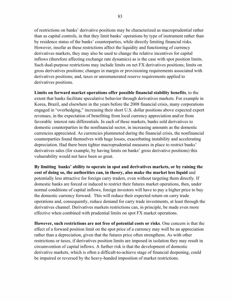
83

of restrictions on banks’ derivative positions may be characterized as macroprudential rather than as capital controls, in that they limit banks’ operations by type of instrument rather than by residence status of the banks’ counterparties, while directly limiting financial risks. However, insofar as these restrictions affect the liquidity and functioning of currency derivatives markets, they may also be used to change the relative incentives for capital inflows (therefore affecting exchange rate dynamics) as is the case with spot position limits. Such dual-purpose restrictions may include limits on net FX derivatives positions; limits on gross derivatives positions; changes in margin or provisioning requirements associated with derivatives positions; and, taxes or unremunerated reserve requirements applied to derivatives positions.

Limits on forward market operations offer possible financial stability benefits, to the extent that banks facilitate speculative behavior through derivatives markets. For example in Korea, Brazil, and elsewhere in the years before the 2008 financial crisis, many corporations engaged in “overhedging,” increasing their short U.S. dollar positions above expected export revenues, in the expectation of benefiting from local currency appreciation and/or from favorable interest rate differentials. In each of these markets, banks sold derivatives to domestic counterparties in the nonfinancial sector, in increasing amounts as the domestic currencies appreciated. As currencies plummeted during the financial crisis, the nonfinancial counterparties found themselves with huge losses, exacerbating instability and accelerating depreciation. Had there been tighter macroprudential measures in place to restrict banks’ derivatives sales (for example, by having limits on banks’ gross derivative positions) this vulnerability would not have been so great.

By limiting banks’ ability to operate in spot and derivatives markets, or by raising the cost of doing so, the authorities can, in theory, also make the market less liquid and potentially less attractive for foreign carry traders, even without targeting them directly. If domestic banks are forced or induced to restrict their futures market operations, then, under normal conditions of capital inflows, foreign investors will have to pay a higher price to buy the domestic currency forward. This will reduce their expected return on carry trade operations and, consequently, reduce demand for carry trade investments, at least through the derivatives channel. Derivatives markets restrictions can, in principle, be made even more effective when combined with prudential limits on spot FX market operations.

However, such restrictions are not free of potential costs or risks. One concern is that the effect of a forward position limit on the spot price of a currency may well be an appreciation rather than a depreciation, given that the futures price often strengthens. As with other restrictions or taxes, if derivatives position limits are imposed in isolation they may result in circumvention of capital inflows. A further risk is that the development of domestic derivative markets, which is often a difficult-to-achieve stage of financial deepening, could be impaired or reversed by the heavy-handed imposition of market restrictions.

84

C. Conclusions

Controlling exchange rate risk is a major task in LA economies. The historical evidence indicates that sharp exchange rate depreciations during crises have often been followed by abrupt appreciations during booming cycles. Such high exchange rate volatility may have detrimental effects on banks’ balance sheets (directly and indirectly through its impact on borrowers’ balance sheets). Central banks and supervisory authorities have sought to lessen these risks through various prudential measures and regulations. Limiting banks’ FX positions is a widespread prudential measure to manage exchange rate risk.

Limits on FX spot positions are valid macroprudential tools when they are use to curb exchange rate volatility and moderate capital inflows. In principle, the limits are macroprudential tools to protect the capital of banks against sudden fluctuations in the exchange rate. However, many countries have actively used them to deliver more exchange rate stability. The tool has been especially valuable during the current cycle in emerging markets, where strong inflows have fed booms in credit and asset prices and generated exchange rate appreciations. Recently, several countries have tightened (or established new) FX position limits to impair the mechanism for carry trade. These regulatory changes has been be part of the toolbox to curb inflows for financial stability purposes, seeking to limit “carry” trades, dampen currency overvaluation, and prevent overly rapid credit growth.

Similarly, there appears to be some scope for the use of macroprudential measures in forward markets to restrain capital inflow pressures. The empirical basis for judging the effectiveness of macroprudential restrictions on forward positions is limited, given that they have not been used with great frequency, and that they are often imposed in conjunction with other measures. However, as with spot position limits, the available evidence suggests that they have the potential to be useful both in protecting financial stability and in shifting the incentives for foreign exchange market arbitrage. In disrupting arbitrage by domestic banks, they can reduce the potential return to carry trade operations. Among the measures that have been implemented, unremunerated reserve requirements based on forward positions appear somewhat more promising than outright limits, given the usual efficiency considerations that apply to the choice between taxes and quotas.10 There also appears to be strong justification for using gross derivatives position limits, possibly in conjunction with net (i.e., derivatives plus spot) FX limits, as a means of controlling specific risks, such as the derivatives carry trade risk. Importantly, the regulatory framework should be carefully designed so that it does not disrupt genuine hedging needs of corporates and other economic agents.

10 An alternative approach, which would also shift marginal incentives without imposing hard limits, would be to increase the risk-based capital charges on banks’ currency derivative positions.

85

Annex 1. Country Experiences and Case Studies This annex surveys the experiences of four countries—Korea, Colombia, Brazil, and Israel—in an effort to ascertain the potential effectiveness of macroprudential restrictions on banks’ spot and derivatives FX positions. Korea and Israel are included because they have experienced capital inflows surges similar to those faced by many Latin American countries While there is an attempt to appraise country experiences analytically, the approach is necessarily somewhat descriptive. The country experiences described are illustrative—this is not meant to be a complete listing of macroprudential FX measures.

Korea Korea, with an export-based economy and a partially open capital account, has often used macro-prudential restrictions on banks' derivative positions in response to capital inflows. In general, it has imposed these restrictions jointly with other prudential measures, or in conjunction with outright capital controls. Two recent instances were in 2004–05, when it imposed a restriction on banks' positions in nondeliverable forward markets, and in 2010, when it limited both net and gross derivative positions.

Korean shipbuilders have strong demands for foreign currency hedging. Korea is the world’s largest shipbuilder by capacity. Given the sector’ long production cycle, shipbuilders generate strong demand for forwards to hedge future export receipts—usually they sell dollars forward and buy Korean won, often with a five year horizon. As described above, this has at times been accompanied by overhedging. The demand for Korean won forwards can stimulate capital inflows, putting upward pressure on the won. Onshore banks, mainly foreign bank branches, have been the dominant providers of FX hedging for exporters. To fund these positions, banks have borrowed U.S. dollars off shore, exchanged them for won in the spot market and invested in Korean won interest rate products on shore (see Annex 2). The rise in banks’ external liabilities added to the already high inflows coming through the equity and bonds markets.

During 2004–05, Korea limited domestic banks' access to the offshore nondeliverable forward (NDF) market in Korean won. At the time, the NDF market was the principal forward market for Korean won, with high liquidity reflecting Korea's position as one of the world's largest exporting nations. Because the won was not (and is not) deliverable offshore, the NDF market also functioned as a proxy spot market for foreign investors desiring exposure to the won but disinclined to bring funds onshore. The Korean authorities were concerned that, as a focus for foreign speculation on the won, the NDF market was driving appreciation in the onshore spot market. To disrupt this process, they imposed restrictions on domestic banks’ NDF positions on January 15, 2004.

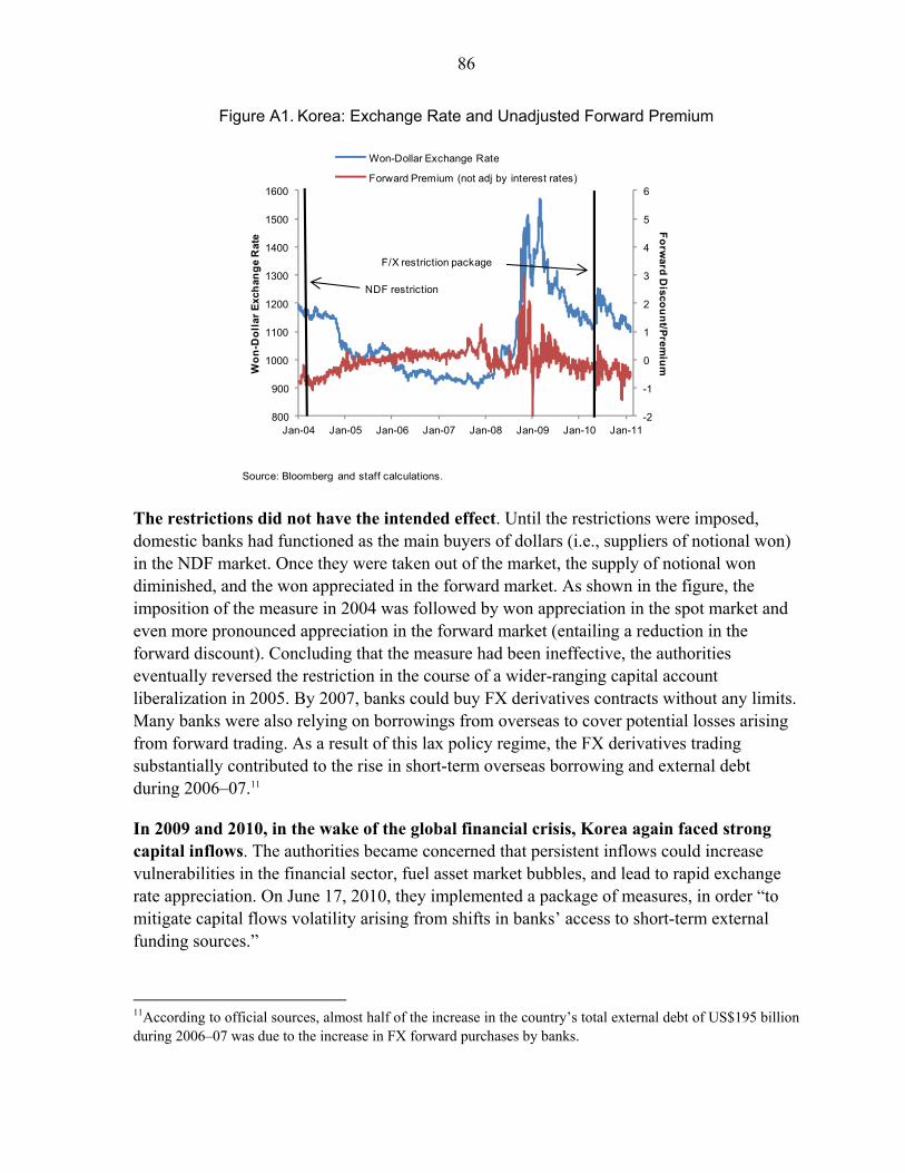
86

Figure A1. Korea: Exchange Rate and Unadjusted Forward Premium

The restrictions did not have the intended effect. Until the restrictions were imposed, domestic banks had functioned as the main buyers of dollars (i.e., suppliers of notional won) in the NDF market. Once they were taken out of the market, the supply of notional won diminished, and the won appreciated in the forward market. As shown in the figure, the imposition of the measure in 2004 was followed by won appreciation in the spot market and even more pronounced appreciation in the forward market (entailing a reduction in the forward discount). Concluding that the measure had been ineffective, the authorities eventually reversed the restriction in the course of a wider-ranging capital account liberalization in 2005. By 2007, banks could buy FX derivatives contracts without any limits. Many banks were also relying on borrowings from overseas to cover potential losses arising from forward trading. As a result of this lax policy regime, the FX derivatives trading substantially contributed to the rise in short-term overseas borrowing and external debt during 2006–07.11

In 2009 and 2010, in the wake of the global financial crisis, Korea again faced strong capital inflows. The authorities became concerned that persistent inflows could increase vulnerabilities in the financial sector, fuel asset market bubbles, and lead to rapid exchange rate appreciation. On June 17, 2010, they implemented a package of measures, in order “to mitigate capital flows volatility arising from shifts in banks’ access to short-term external funding sources.”

11According to official sources, almost half of the increase in the country’s total external debt of US$195 billion during 2006–07 was due to the increase in FX forward purchases by banks.

-2

-1

0

1

2

3

4

5

6

800

900

1000

1100

1200

1300

1400

1500

1600

Jan-04 Jan-05 Jan-06 Jan-07 Jan-08 Jan-09 Jan-10 Jan-11

Fo

rwa

rd D

isco

un

t/Pre

miu

mW

on

-Do

llar

Ex

chan

ge

Ra

te

Won-Dollar Exchange Rate

Forward Premium (not adj by interest rates)

NDF restriction

F/X restriction package

Source: Bloomberg and staff calculations.

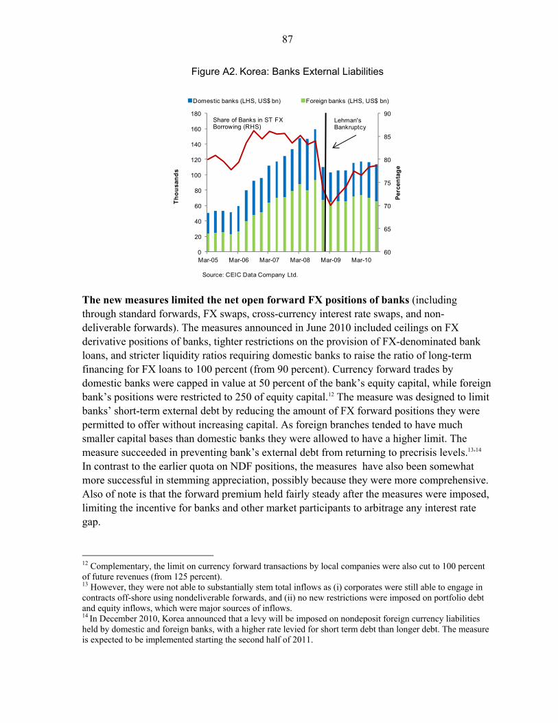
87

Figure A2. Korea: Banks External Liabilities

The new measures limited the net open forward FX positions of banks (including through standard forwards, FX swaps, cross-currency interest rate swaps, and non-deliverable forwards). The measures announced in June 2010 included ceilings on FX derivative positions of banks, tighter restrictions on the provision of FX-denominated bank loans, and stricter liquidity ratios requiring domestic banks to raise the ratio of long-term financing for FX loans to 100 percent (from 90 percent). Currency forward trades by domestic banks were capped in value at 50 percent of the bank’s equity capital, while foreign bank’s positions were restricted to 250 of equity capital.12 The measure was designed to limit banks’ short-term external debt by reducing the amount of FX forward positions they were permitted to offer without increasing capital. As foreign branches tended to have much smaller capital bases than domestic banks they were allowed to have a higher limit. The measure succeeded in preventing bank’s external debt from returning to precrisis levels.13,14 In contrast to the earlier quota on NDF positions, the measures have also been somewhat more successful in stemming appreciation, possibly because they were more comprehensive. Also of note is that the forward premium held fairly steady after the measures were imposed, limiting the incentive for banks and other market participants to arbitrage any interest rate gap.

12 Complementary, the limit on currency forward transactions by local companies were also cut to 100 percent of future revenues (from 125 percent). 13 However, they were not able to substantially stem total inflows as (i) corporates were still able to engage in contracts off-shore using nondeliverable forwards, and (ii) no new restrictions were imposed on portfolio debt and equity inflows, which were major sources of inflows. 14 In December 2010, Korea announced that a levy will be imposed on nondeposit foreign currency liabilities held by domestic and foreign banks, with a higher rate levied for short term debt than longer debt. The measure is expected to be implemented starting the second half of 2011.

60

65

70

75

80

85

90

0

20

40

60

80

100

120

140

160

180

Mar-05 Mar-06 Mar-07 Mar-08 Mar-09 Mar-10

Per

cen

tag

e

Th

ou

san

ds

Domestic banks (LHS, US$ bn) Foreign banks (LHS, US$ bn)

Share of Banks in ST FX Borrowing (RHS)

Lehman's Bankruptcy

Source: CEIC Data Company Ltd.

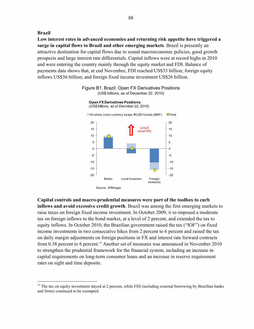
88

Brazil Low interest rates in advanced economies and returning risk appetite have triggered a surge in capital flows to Brazil and other emerging markets. Brazil is presently an attractive destination for capital flows due to sound macroeconomic policies, good growth prospects and large interest rate differentials. Capital inflows were at record highs in 2010 and were entering the country mainly through the equity market and FDI. Balance of payments data shows that, at end November, FDI reached US$33 billion; foreign equity inflows US$36 billion; and foreign fixed income investment US$26 billion.

Figure B1. Brazil: Open FX Derivatives Positions (US$ billions, as of December 22, 2010)

Capital controls and macro-prudential measures were part of the toolbox to curb inflows and avoid excessive credit growth. Brazil was among the first emerging markets to raise taxes on foreign fixed income investment. In October 2009, it re-imposed a moderate tax on foreign inflows to the bond market, at a level of 2 percent, and extended the tax to equity inflows. In October 2010, the Brazilian government raised the tax (“IOF”) on fixed income investments in two consecutive hikes from 2 percent to 6 percent and raised the tax on daily margin adjustments on foreign positions in FX and interest rate forward contracts from 0.38 percent to 6 percent.15 Another set of measures was announced in November 2010 to strengthen the prudential framework for the financial system, including an increase in capital requirements on long-term consumer loans and an increase in reserve requirement rates on sight and time deposits.

15 The tax on equity investment stayed at 2 percent, while FDI (including external borrowing by Brazilian banks and firms) continued to be exempted.

-20

-15

-10

-5

0

5

10

15

20

-20

-15

-10

-5

0

5

10

15

20

Banks Local investors Foreign investors

On-shore cross currency swaps USD futures (BMF) Total

Long $(short R$)

Open FX Derivatives Positions(US$ billions, as of Decmber 22, 2010)

Source: JPMorgan

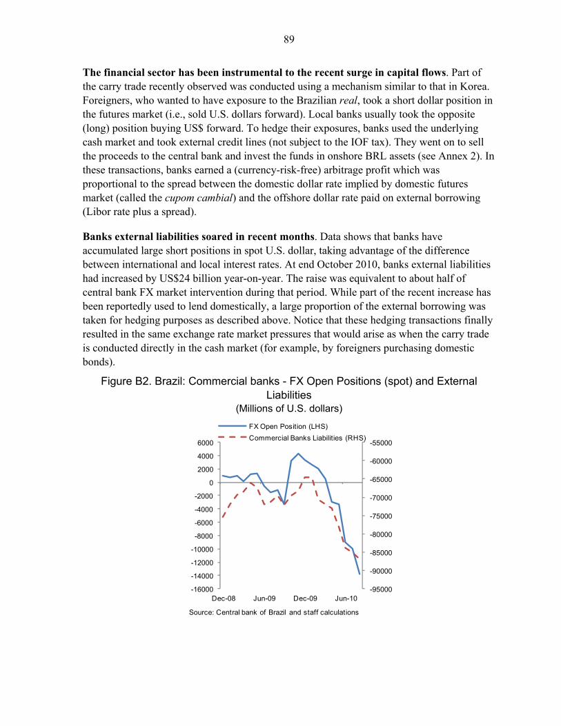
89

The financial sector has been instrumental to the recent surge in capital flows. Part of the carry trade recently observed was conducted using a mechanism similar to that in Korea. Foreigners, who wanted to have exposure to the Brazilian real, took a short dollar position in the futures market (i.e., sold U.S. dollars forward). Local banks usually took the opposite (long) position buying US$ forward. To hedge their exposures, banks used the underlying cash market and took external credit lines (not subject to the IOF tax). They went on to sell the proceeds to the central bank and invest the funds in onshore BRL assets (see Annex 2). In these transactions, banks earned a (currency-risk-free) arbitrage profit which was proportional to the spread between the domestic dollar rate implied by domestic futures market (called the cupom cambial) and the offshore dollar rate paid on external borrowing (Libor rate plus a spread).

Banks external liabilities soared in recent months. Data shows that banks have accumulated large short positions in spot U.S. dollar, taking advantage of the difference between international and local interest rates. At end October 2010, banks external liabilities had increased by US$24 billion year-on-year. The raise was equivalent to about half of central bank FX market intervention during that period. While part of the recent increase has been reportedly used to lend domestically, a large proportion of the external borrowing was taken for hedging purposes as described above. Notice that these hedging transactions finally resulted in the same exchange rate market pressures that would arise as when the carry trade is conducted directly in the cash market (for example, by foreigners purchasing domestic bonds).

Figure B2. Brazil: Commercial banks - FX Open Positions (spot) and External Liabilities

(Millions of U.S. dollars)

-95000

-90000

-85000

-80000

-75000

-70000

-65000

-60000

-55000

-16000

-14000

-12000

-10000

-8000

-6000

-4000

-2000

0

2000

4000

6000

Dec-08 Jun-09 Dec-09 Jun-10

FX Open Position (LHS)

Commercial Banks Liabilities (RHS)

Source: Central bank of Brazil and staff calculations

90

External borrowing was not constrained by existing regulatory limits on net open FX positions. Current regulations state that a bank’s net open position, including spot and derivative transactions, should be at most 30 percent of capital. Since the transactions supporting the carry trade involved assuming both a long (in the futures market) and short (in the spot market) FX position, they cancelled out when calculating net open positions. The net open position limits were clearly not binding. Banks short positions (as percentage of capital) barely fluctuated in recent months and remained very small compared to the short position limit.16

Changes in the regulatory framework would help to moderate capital inflows and prevent the building-up of vulnerabilities in the banking sector. The carry trade relies on the domestic banks’ ability to increase their short spot position in the FX market (i.e. to borrow in FX) as a hedge to their positions in the futures markets. Changes in regulations could be targeted at limiting this ability, reducing the vulnerabilities associated with the bank’s intermediation role between the futures and spot markets.

Prudential measures could also target banks’ ability to increase their net FX derivative position. Possible alternatives include: a general tax on banks' derivatives margin positions, a limit on gross derivatives positions, or a tax on gross derivatives positions. Each of these would be likely to have some effect on arbitrage.17 Banks that are naturally long dollars in the futures market would be less inclined to purchase dollars forward at any given price, and therefore less inclined to borrow dollars in the spot market. In an environment of persistent capital inflows, this would mean a widening of the basis spread,18 making it less attractive for market participants in Brazil to engage in synthetic dollar borrowing operations. Taxes or restrictions on forex futures positions would target more directly the mechanics of carry trade in the futures market and may be perceived as being less intrusive toward the banks’ other commercial functions.19

Colombia Faced with heavy capital inflows and rapid appreciation, on May 6, 2007 Colombia imposed a restriction on banks’ gross currency derivative positions, limiting them to 500 percent of capital on both the short and long sides. At the same time, the central bank imposed an unremunerated reserve requirement on banks’ external borrowing. The two

16 The net open position of the banking system has remained usually below 6 percent of capital since 2008. 17 Thus, instead of having an overall net open position limit (including spot and derivative operations), banks would be subject to separated quantitative limits for these two types of transactions. 18 That is an increase in the interest-rate-adjusted forward premium. 19 Alternatively, authorities could impose a levy on foreign borrowing or subject these external funds to some kind of unremunerated reserve requirements. The disadvantage of a reserve requirements policy is that it would affect the total amount of external borrowing and, therefore, would make hedging more costly for all agents (including those not having a speculative purpose, like exporters). The Brazilian central bank recently implemented a measure requiring banks to deposit the equivalent of 60 percent of their short spot dollar positions in cash at the central bank, at no interest. This requirement applies to the amount that exceeds US$3 billion or Tier I capital, whichever is lower.

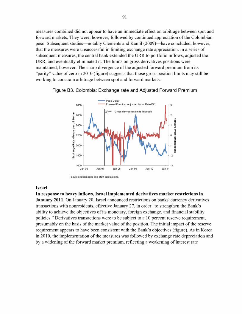
91

measures combined did not appear to have an immediate effect on arbitrage between spot and forward markets. They were, however, followed by continued appreciation of the Colombian peso. Subsequent studies––notably Clements and Kamil (2009)—have concluded, however, that the measures were unsuccessful in limiting exchange rate appreciation. In a series of subsequent measures, the central bank extended the URR to portfolio inflows, adjusted the URR, and eventually eliminated it. The limits on gross derivatives positions were maintained, however. The sharp divergence of the adjusted forward premium from its “parity” value of zero in 2010 (figure) suggests that those gross position limits may still be working to constrain arbitrage between spot and forward markets.

Figure B3. Colombia: Exchange rate and Adjusted Forward Premium

Israel In response to heavy inflows, Israel implemented derivatives market restrictions in January 2011. On January 20, Israel announced restrictions on banks' currency derivatives transactions with nonresidents, effective January 27, in order “to strengthen the Bank’s ability to achieve the objectives of its monetary, foreign exchange, and financial stability policies.” Derivatives transactions were to be subject to a 10 percent reserve requirement, presumably on the basis of the market value of the position. The initial impact of the reserve requirement appears to have been consistent with the Bank’s objectives (figure). As in Korea in 2010, the implementation of the measures was followed by exchange rate depreciation and by a widening of the forward market premium, reflecting a weakening of interest rate

-3

-2

-1

0

1

2

3

1600

1800

2000

2200

2400

2600

2800

Jan-06 Jan-07 Jan-08 Jan-09 Jan-10 Jan-11

Fo

rward

Prem

ium

/Disco

un

t

Ex

chan

ge

Ra

te -

Pe

sos

per

US

Do

llar

Peso-DollarForward Premium Adjusted by Int Rate Diff

Gross derivatives limits imposed

Source: Bloomberg and staff calculations.

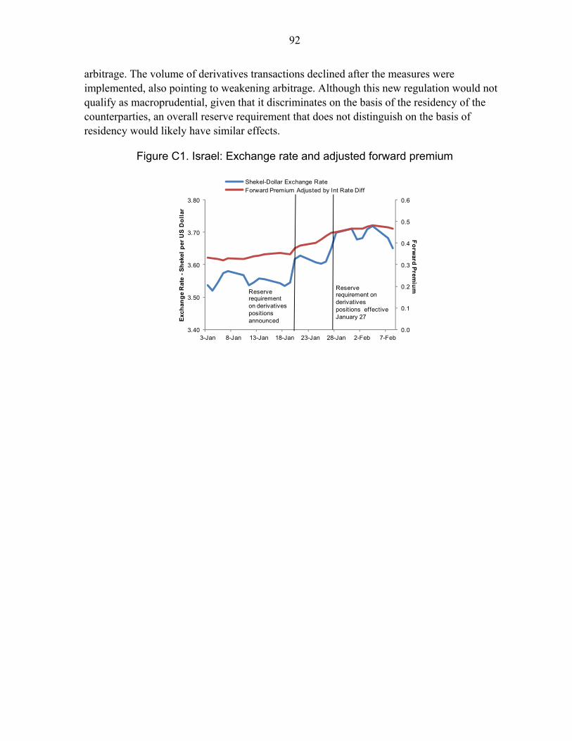
92

arbitrage. The volume of derivatives transactions declined after the measures were implemented, also pointing to weakening arbitrage. Although this new regulation would not qualify as macroprudential, given that it discriminates on the basis of the residency of the counterparties, an overall reserve requirement that does not distinguish on the basis of residency would likely have similar effects.

Figure C1. Israel: Exchange rate and adjusted forward premium

0.0

0.1

0.2

0.3

0.4

0.5

0.6

3.40

3.50

3.60

3.70

3.80

3-Jan 8-Jan 13-Jan 18-Jan 23-Jan 28-Jan 2-Feb 7-Feb

Fo

rward

Prem

ium

Exc

han

ge

Rat

e -S

hek

el p

er U

S D

oll

arShekel-Dollar Exchange RateForward Premium Adjusted by Int Rate Diff

Reserve requirement on derivativespositions announced

Reserve requirement on derivativespositions effective January 27

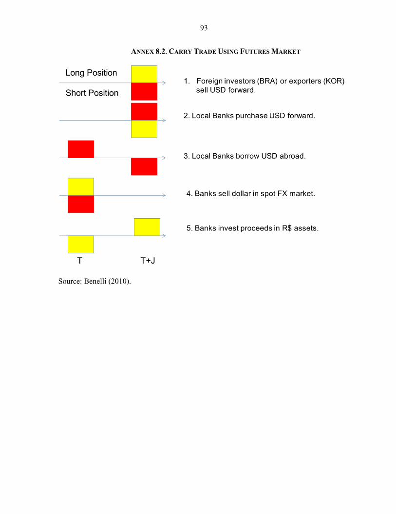
93

ANNEX 8.2. CARRY TRADE USING FUTURES MARKET

Source: Benelli (2010).

1. Foreign investors (BRA) or exporters (KOR)sell USD forward.

2. Local Banks purchase USD forward.

3. Local Banks borrow USD abroad.

4. Banks sell dollar in spot FX market.

5. Banks invest proceeds in R$ assets.

Long Position

Short Position

T T+J

94

IX. RESERVE REQUIREMENTS AND TAXES ON CAPITAL INFLOWS1,2

A. Introduction

Countries have used reserve requirements on capital inflows in response to a surge in capital inflows. Policy makers may require that a fraction of the private capital inflows from nonresidents—be deposited at the central bank for a period of time. At the end of the holding period, these deposits—which are known as reserve requirements (RRs)—are reimbursed along with any applicable remuneration. In general, RRs are usually unremunerated (URR).

RRs on capital inflows act as a price-based capital account restriction. In addition to limiting liquidity for foreign investors in the country, as RRs are either unremunerated or remunerated below market rates, RRs increase the cost of cross-border financing making domestic investment opportunities less attractive to foreign investors—in particular, for short-term investments. The cost of setting RRs on capital inflows can be expressed in terms of a tax-equivalent with analogous impact to an explicit tax on flows from non-residents, such as the Brazilian Imposto de Operações Financeiras (IOF) (which is also covered in this note).3 Further, the RR regulation could give investors the option of paying an up-front fee—equivalent or marginally higher than the foregone interest—for an early withdrawal of the deposit.

RRs on capital inflows can serve macroprudential purposes:

First, RRs could have a countercyclical impact during periods of easy and transitory global financing. If applied broadly across types of inflows and succeed in reducing total capital inflows, RRs could limit excessive and unsustainable foreign leverage, and in turn, limit the impact on flows absorption.

Second, RRs may help contain systemic and liquidity risk. By tilting foreign funding towards longer maturities, the funding structure of domestic corporates improves and becomes less vulnerable to sudden capital reversals.

Third, RRs can also help the central bank gain space for raising domestic interest rates without encouraging massive capital inflows into the country. The reason is that by increasing the cost of foreign capital, RRs sever the arbitrage link between domestic and international interest rates.

1 Prepared by Mercedes Garcia-Escribano. Comments by C. Tovar and M.K. Tang are acknowledged. 2 The instruments described in this chapter could be referred to as “residency-based capital flow management measures” according to the nomenclature in IMF, 2011e. 3 Given the similarity between RRs on capital inflows and inflow taxes, administrative considerations determine the choice. In particular, while the central bank may have the authority to impose URRs, it does not have authority to levy taxes (Ostry et al., 2011).

95

Last, they could also eliminate or reduce the quasi-fiscal costs associated with sterilized foreign-exchange intervention.

However, there are costs associated to the RRs.4 First, their effectiveness to limit capital inflows, if any, is transitory. Following the introduction of RRs on inflows, investors may try to find alternative capital account channels or instruments to bypass regulations, so RRs gradually loose power. Thus, an ongoing effort to tighten the policy and its administration—for example, raising the fraction that has to be deposited at the central bank or broadening the types of inflows subject to the RRs—may be needed to maintain their impact. Further, the alternative instruments used by investors may cause the buildup of vulnerabilities and foster future potential crisis. Moreover, their design and administration is complex. Another risk associated to RRs is that they be perceived as a regime change for a country, which could trigger a sudden and sharp decline in foreign financing and divert flows to other countries. For these reasons, the RRs on inflows should only be considered when other options for dealing with the inflows have already been deployed or are infeasible (IMF, 2011e).

Taking into account these caveats, countries that have deployed RR on inflows have tailored them to their circumstances. The RRs could apply to all flows or differentiate by type of flow (foreign borrowing, portfolio inflows and direct investment) and duration of the flow (short-term and medium-long term). RRs also differ in the holding period, the fraction of the flow that has to be deposited at the central bank, and the remuneration rate (if any). The currency denomination of the reserve requirement could also be a variable of choice for the investor or the authority. The Annex describes the forms that RRs on capital inflows have taken across countries in Latin America:5 URRs on foreign borrowing in Chile, URRs on foreign borrowing and portfolio inflows in Colombia, URRs on deposits in local currency from nonresident financial institutions in Peru;6 and the Brazilian IOF. It is important to note that RRs on capital inflows have usually been introduced in combination with other policies or measures to limit capital inflows.7

B. Theoretical Considerations

The economic effect of the reserve requirement on capital inflows can be derived in terms of the implied tax-equivalent cost. In the presence of RRs, a risk-neutral investor will face an additional cost when choosing to hold domestic assets. Or put it differently, RRs 4 See Eyzaguirre et al., 2011. 5 Other countries that deployed RRs on capital inflows include Thailand during 2006–08, Russia during 2004–06, and Malaysia in 1994. 6 Reserve requirements on bank deposits that discriminate in terms of residency are covered in this chapter, while those that differentiate in terms of the currency of denomination are described in Chapter VI on reserve requirements on bank liabilities. This classification is consistent with that presented in IMF, 2011k and Ostry et al., 2011. 7 For example, in 1994 Malaysia (i) required that commercial banks placed with the central bank the ringgit funds of foreign banks in non-interest bearing accounts, and also (ii) prohibited residents from selling short-term monetary instruments to nonresidents, and (iii) introduced asymmetric open position limits.

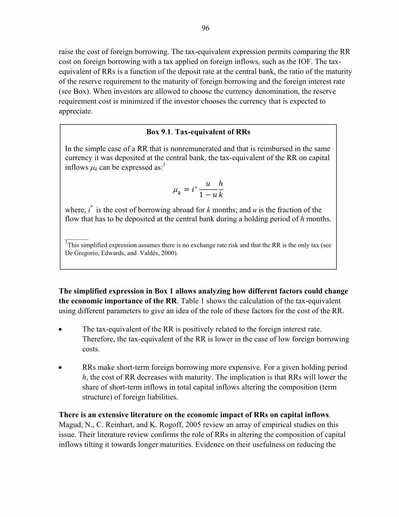
96

raise the cost of foreign borrowing. The tax-equivalent expression permits comparing the RR cost on foreign borrowing with a tax applied on foreign inflows, such as the IOF. The tax-equivalent of RRs is a function of the deposit rate at the central bank, the ratio of the maturity of the reserve requirement to the maturity of foreign borrowing and the foreign interest rate (see Box). When investors are allowed to choose the currency denomination, the reserve requirement cost is minimized if the investor chooses the currency that is expected to appreciate.

The simplified expression in Box 1 allows analyzing how different factors could change the economic importance of the RR. Table 1 shows the calculation of the tax-equivalent using different parameters to give an idea of the role of these factors for the cost of the RR.

The tax-equivalent of the RR is positively related to the foreign interest rate. Therefore, the tax-equivalent of the RR is lower in the case of low foreign borrowing costs.

RRs make short-term foreign borrowing more expensive. For a given holding period h, the cost of RR decreases with maturity. The implication is that RRs will lower the share of short-term inflows in total capital inflows altering the composition (term structure) of foreign liabilities.

There is an extensive literature on the economic impact of RRs on capital inflows. Magud, N., C. Reinhart, and K. Rogoff, 2005 review an array of empirical studies on this issue. Their literature review confirms the role of RRs in altering the composition of capital inflows tilting it towards longer maturities. Evidence on their usefulness on reducing the

1

Box 9.1. Tax-equivalent of RRs

In the simple case of a RR that is nonremunerated and that is reimbursed in the same currency it was deposited at the central bank, the tax-equivalent of the RR on capital inflows k can be expressed as:1

where, i* is the cost of borrowing abroad for k months; and u is the fraction of the flow that has to be deposited at the central bank during a holding period of h months.

______ 1This simplified expression assumes there is no exchange rate risk and that the RR is the only tax (see De Gregorio, Edwards, and Valdés, 2000).

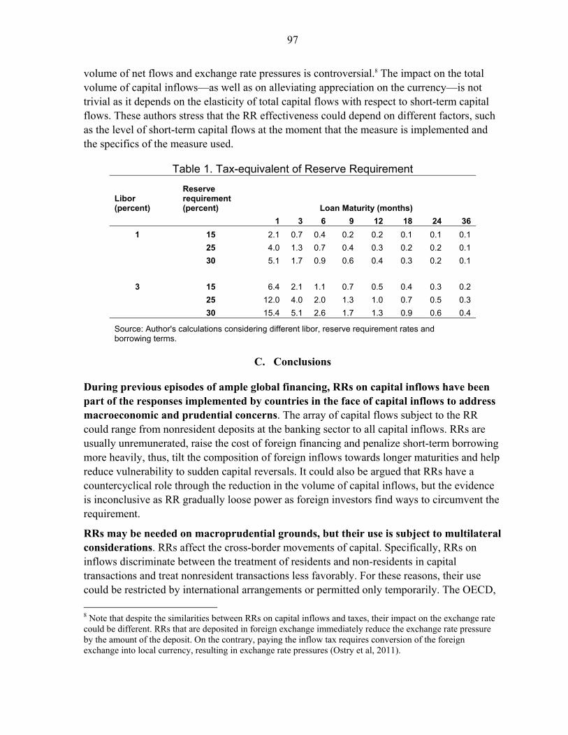
97

volume of net flows and exchange rate pressures is controversial.8 The impact on the total volume of capital inflows—as well as on alleviating appreciation on the currency—is not trivial as it depends on the elasticity of total capital flows with respect to short-term capital flows. These authors stress that the RR effectiveness could depend on different factors, such as the level of short-term capital flows at the moment that the measure is implemented and the specifics of the measure used.

Table 1. Tax-equivalent of Reserve Requirement

Libor (percent)

Reserve requirement (percent) Loan Maturity (months)

1 3 6 9 12 18 24 36

1 15 2.1 0.7 0.4 0.2 0.2 0.1 0.1 0.1

25 4.0 1.3 0.7 0.4 0.3 0.2 0.2 0.1

30 5.1 1.7 0.9 0.6 0.4 0.3 0.2 0.1

3 15 6.4 2.1 1.1 0.7 0.5 0.4 0.3 0.2

25 12.0 4.0 2.0 1.3 1.0 0.7 0.5 0.3

30 15.4 5.1 2.6 1.7 1.3 0.9 0.6 0.4

Source: Author's calculations considering different libor, reserve requirement rates and borrowing terms.

C. Conclusions

During previous episodes of ample global financing, RRs on capital inflows have been part of the responses implemented by countries in the face of capital inflows to address macroeconomic and prudential concerns. The array of capital flows subject to the RR could range from nonresident deposits at the banking sector to all capital inflows. RRs are usually unremunerated, raise the cost of foreign financing and penalize short-term borrowing more heavily, thus, tilt the composition of foreign inflows towards longer maturities and help reduce vulnerability to sudden capital reversals. It could also be argued that RRs have a countercyclical role through the reduction in the volume of capital inflows, but the evidence is inconclusive as RR gradually loose power as foreign investors find ways to circumvent the requirement.

RRs may be needed on macroprudential grounds, but their use is subject to multilateral considerations. RRs affect the cross-border movements of capital. Specifically, RRs on inflows discriminate between the treatment of residents and non-residents in capital transactions and treat nonresident transactions less favorably. For these reasons, their use could be restricted by international arrangements or permitted only temporarily. The OECD,

8 Note that despite the similarities between RRs on capital inflows and taxes, their impact on the exchange rate could be different. RRs that are deposited in foreign exchange immediately reduce the exchange rate pressure by the amount of the deposit. On the contrary, paying the inflow tax requires conversion of the foreign exchange into local currency, resulting in exchange rate pressures (Ostry et al, 2011).

98

EU, GATs and (Bilateral Investment Treaties) BITS allow for the temporary implementation of restrictions to the movement of capital flows in case of “serious economic and financial disturbances” or “serious balance of payments”.

There are additional costs associated to the implementation of RRs. RRs may create an incentive for investors to rely on alternative and complex investment instruments that could foster the buildup of capital account and financial vulnerabilities. Also, their implementation could be perceived by investors as a regime change for a country leading to a decline of stable and long term capital flows. Therefore, preference should be given to other measures that impact capital inflows but do not discriminate on the basis of residency (IMF, 2011f).

Amidst the current surge in capital inflows, so far, only a few countries in Latin America have redeployed RRs on inflows. Peru has raised the RR rate on nonresidents bank deposits more than the RR rate applicable to residents’ deposits, while Brazil has reinstituted the IOF as part of its response to avoid excessive reliance on foreign financing.

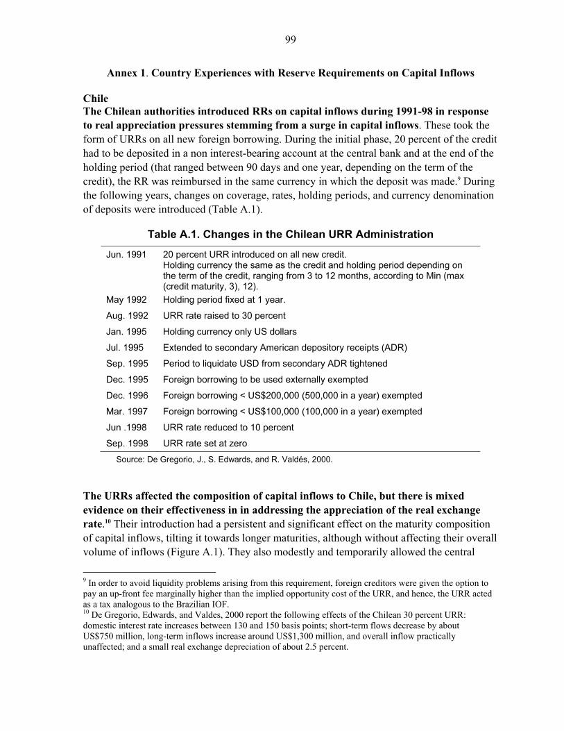
99

Annex 1. Country Experiences with Reserve Requirements on Capital Inflows Chile The Chilean authorities introduced RRs on capital inflows during 1991-98 in response to real appreciation pressures stemming from a surge in capital inflows. These took the form of URRs on all new foreign borrowing. During the initial phase, 20 percent of the credit had to be deposited in a non interest-bearing account at the central bank and at the end of the holding period (that ranged between 90 days and one year, depending on the term of the credit), the RR was reimbursed in the same currency in which the deposit was made.9 During the following years, changes on coverage, rates, holding periods, and currency denomination of deposits were introduced (Table A.1).

Table A.1. Changes in the Chilean URR Administration

Jun. 1991 20 percent URR introduced on all new credit. Holding currency the same as the credit and holding period depending on the term of the credit, ranging from 3 to 12 months, according to Min (max (credit maturity, 3), 12).

May 1992 Holding period fixed at 1 year.

Aug. 1992 URR rate raised to 30 percent

Jan. 1995 Holding currency only US dollars

Jul. 1995 Extended to secondary American depository receipts (ADR)

Sep. 1995 Period to liquidate USD from secondary ADR tightened

Dec. 1995 Foreign borrowing to be used externally exempted

Dec. 1996 Foreign borrowing < US$200,000 (500,000 in a year) exempted

Mar. 1997 Foreign borrowing < US$100,000 (100,000 in a year) exempted

Jun .1998 URR rate reduced to 10 percent

Sep. 1998 URR rate set at zero

Source: De Gregorio, J., S. Edwards, and R. Valdés, 2000.

The URRs affected the composition of capital inflows to Chile, but there is mixed evidence on their effectiveness in in addressing the appreciation of the real exchange rate.10 Their introduction had a persistent and significant effect on the maturity composition of capital inflows, tilting it towards longer maturities, although without affecting their overall volume of inflows (Figure A.1). They also modestly and temporarily allowed the central

9 In order to avoid liquidity problems arising from this requirement, foreign creditors were given the option to pay an up-front fee marginally higher than the implied opportunity cost of the URR, and hence, the URR acted as a tax analogous to the Brazilian IOF. 10 De Gregorio, Edwards, and Valdes, 2000 report the following effects of the Chilean 30 percent URR: domestic interest rate increases between 130 and 150 basis points; short-term flows decrease by about US$750 million, long-term inflows increase around US$1,300 million, and overall inflow practically unaffected; and a small real exchange depreciation of about 2.5 percent.

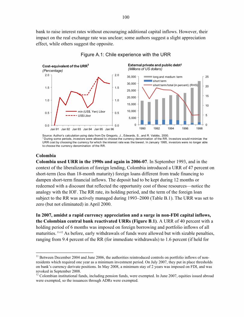
100

bank to raise interest rates without encouraging additional capital inflows. However, their impact on the real exchange rate was unclear; some authors suggest a slight appreciation effect, while others suggest the opposite.

Figure A.1: Chile experience with the URR

Colombia Colombia used URR in the 1990s and again in 2006-07. In September 1993, and in the context of the liberalization of foreign lending, Colombia introduced a URR of 47 percent on short-term (less than 18-month maturity) foreign loans different from trade financing to dampen short-term financial inflows. The deposit had to be kept during 12 months or redeemed with a discount that reflected the opportunity cost of those resources—notice the analogy with the IOF. The RR rate, its holding period, and the term of the foreign loan subject to the RR was actively managed during 1993–2000 (Table B.1). The URR was set to zero (but not eliminated) in April 2000.

In 2007, amidst a rapid currency appreciation and a surge in non-FDI capital inflows, the Colombian central bank reactivated URRs (Figure B.1). A URR of 40 percent with a holding period of 6 months was imposed on foreign borrowing and portfolio inflows of all maturities. 11,12 As before, early withdrawals of funds were allowed but with sizable penalties, ranging from 9.4 percent of the RR (for immediate withdrawals) to 1.6 percent (if held for

11 Between December 2004 and June 2006, the authorities reintroduced controls on portfolio inflows of non-residents which required one year as a minimum investment period. On July 2007, they put in place thresholds on bank’s currency derivate positions. In May 2008, a minimum stay of 2 years was imposed on FDI, and was revoked in September 2008. 12 Colombian institutional funds, including pension funds, were exempted. In June 2007, equities issued abroad were exempted, so the issuances through ADRs were exempted.

0.0

0.5

1.0

1.5

2.0

0.0

0.5

1.0

1.5

2.0

Jan 91 Jan 92 Jan 93 Jan 94 Jan 95 Jan 96

min (US$, Yen) Libor

US$ Libor

Cost-equivalent of the URR¹(Percentage)

Source: Author’s calculation using data from De Gregorio, J., Edwards, S., and R. Valdés, 2000.1 During some periods, investors were allowed to choose the currency denomination of the RR. Investors would minimize the URR cost by choosing the currency for which the interest rate was the lowest. In January 1995, investors were no longer able to choose the currency denomination of the RR.

External private and public debt2

(Millions of US dollars)

0

5

10

15

20

25

0

5,000

10,000

15,000

20,000

25,000

30,000

35,000

1990 1992 1994 1996 1998

long and medium term

short term

short term/total (in percent) (RHS)

101

5 months). URRs were loosened in December 2007, tightened back in May 2008 and again loosened in September 2008.13 The URR rate was set down to zero in October 2008.

Table B.1. Changes in the Colombian URR Administration

Date

Maximum Term for the Loan Subject to

the Deposit (Months)

Reserve Requirements (Percent)

Holding Period

(Months) Currency

Sep. 1993 18 47 12 USD

Mar. 1994 36 93 for loans with maturities up to 1 year

12 USD

64 for loans with maturities up to 2 years

18 USD

50 for loans with maturities up to 3 years

24 USD

Aug. 1994 60 140 for loans maturing in less than 1 month

1 USD

… … USD

42.8 for loans maturing in 60 months

60 USD

Feb. 1996 48 85 6 USD

… … USD

10 48 USD

Mar. 1996 36 50 18 USD

Mar. 1997 1/

60 50 18 USD

Mar. 1997 All 30 18 USD & Pesos

Jan. 1998 All 25 12 Pesos

Sep. 1998 All 10 6 Pesos

Apr. 2000 All 0 0 ---

May 2007 All 40 6 Pesos

May 2008 All 50 6 Pesos

Oct .2008 All 0 0 --- Source: Rincon, and Toro, 2010, and Ocampo and Tovar, 2003. 1 In addition to the RR, in January 1997, an explicit (Tobin) tax on all capital flows was introduced. It was short-lived as it was decreed unconstitutional in March 1007.

Colombia’s experience with URRs was successful in altering the composition of capital inflows, but did not have a significant impact on reducing the volume of inflows or

13 In December 2007, the penalties for early withdrawal of funds were reduced and the initial public offerings of equities were exempted from the URR. The URR on portfolio inflows was raised from 40 to 50 percent in May 2008, and in June, the penalty for early withdrawal of deposits was raised. In September 2008, URR was loosened as purchases of equities were exempted.

102

modifying the level of the exchange. Most studies on the 1990s URRs experience conclude that they were effective in reducing short-term flows with mixed results on the impact on total capital flows. For example, Ocampo and Tovar (2003) argue that restrictions diminished not only short-term but also long-term capital flows. Studies on the most recent 2007 experience also find a significant effect on short-term capital inflows. Clements and Kamil (2009) find significant reductions in foreign borrowing and non-resident portfolio inflows, and no impact on total net private capital movements. Clements and Kamil (2009) and Rincon and Toro (2010) find an increased the volatility of the exchange rate but no evidence of diminished appreciation pressures.14

Figure B.1: Colombia’s Experience with the URR

Peru The central bank of Peru has actively used RRs on bank deposits from non-resident financial institutions during 2008 and again since early-2010. Amidst the surge in capital inflows during 2008, the central bank increased the minimum and marginal reserve requirements on deposits, but even more so the marginal rate applying to deposits from the following foreign institutions: financial institutions, hedge funds, pension funds, brokers, mutual funds and investment banks.15 However, these measures proved to be temporary as they were eliminated in late 2008 following Lehmann’s collapse. In early 2010, renewed inflows led the central bank to impose again marginal reserve requirement on deposits from non-resident financial institution at levels similar to those of mid-2008 (see a summary of measures adopted in Figure C.1). Peru’s use of RRs was effective in altering the composition 14 Clements and Kamil (2009) explain that the increased exchange rate volatility could be due to the fact that the URR placed the pension funds in a privileged position, as they were excluded from the restrictions, and hence, increased the importance of domestic pension funds in exchange rate market trading. 15 In addition to the RR management, the central bank rose the RR on short-term foreign liabilities and introduced a fee to the transfer of Bank certificates.

Cost-equivalent of the URR¹(Percentage)

Source: Left-hand panel: author’s calculation using data from Rincon, H. and J. Toro, 2010. Right-hand panel: Author’s calculation using data from Ocampo and Tovar, 2003.

External private debt2

(Millions of US dollars)

0

20

40

60

80

100

120

140

160

0

20

40

60

80

100

120

140

160

1993 1996 1999 2002 2005 20080

20

40

60

80

100

0

20

40

60

80

100

1990199119921993199419951996199719981999

Long-term Short-term

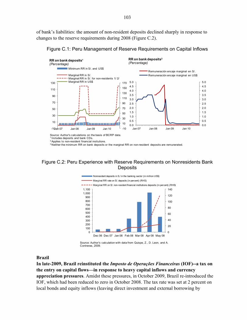
103

of bank’s liabilities: the amount of non-resident deposits declined sharply in response to changes to the reserve requirements during 2008 (Figure C.2).

Figure C.1: Peru Management of Reserve Requirements on Capital Inflows

Figure C.2: Peru Experience with Reserve Requirements on Nonresidents Bank Deposits

Brazil In late-2009, Brazil reinstituted the Imposto de Operações Financeiras (IOF)--a tax on the entry on capital flows—in response to heavy capital inflows and currency appreciation pressures. Amidst these pressures, in October 2009, Brazil re-introduced the IOF, which had been reduced to zero in October 2008. The tax rate was set at 2 percent on local bonds and equity inflows (leaving direct investment and external borrowing by

-10

10

30

50

70

90

110

130

150

170

-10

10

30

50

70

90

110

130


Minimum RR in S/. and US$

Marginal RR in S/.Marginal RR in S/. for non-residents 1/ 2/Marginal RR in US$

0.0

0.5

1.0

1.5

2.0

2.5

3.0

3.5

4.0

4.5

5.0

0.0

0.5

1.0

1.5

2.0

2.5

3.0

3.5

4.0

4.5

5.0


Remuneración encaje marginal en S/.

Remuneración encaje marginal en US$

RR on bank deposits¹ (Percentage)

RR on bank deposits3

(Percentage)

Source: Author's calculations on the basis of BCRP data.1 Includes deposits and bank CDs.2 Applies to non-resident financial insitutions.3 Neither the minimum RR on bank deposits or the marginal RR on non-resident deposits are remunerated.

0

20

40

60

80

100

120

140

0

100

200

300

400

500

600

700

800

900

1,000

1,100

Dec 06 Dec 07 Jan 08 Feb 08 Mar 08 Apr 08 May 08

Nonresident deposits in S./ in the banking sector (in million US$)

Marginal RR rate on S/. deposits (in percent) (RHS)

Marginal RR on S/. non-resident financial institutions deposits (in percent) (RHS)

Source: Author’s calculation with data from Quispe, Z., D. Leon, and A. Contreras, 2009.

104

Brazilian banks and firms not directly affected by the tax) compared to 1½ percent rate only on fixed income in the previous year. On the day following the reintroduction of the IOF, the Brazilian real, which had appreciated by 35 percent against the U.S. dollar since the beginning of this year, depreciated by about 2 percent (to R$1.75 to the dollar) but quickly afterwards resumed its appreciation trend. In October 2010, the IOF tax on foreign investment in local bonds was raised to 4 percent from 2 percent while tax rate for the purchase of Brazilian stocks by foreigners was left at 2 percent. A few weeks later, the tax rate on fixed-income was raised again to 6 percent from 4 percent. The re-introduction of the IOF may have changed the composition of capital inflows, while its impact on the total volume of capital inflows was debatable (Walker, 2010). Equity flows did diminish after the IOF was re-introduced in October 2009, while inflows into domestic bonds remained quite robust. Walker (2010) shows that the IOF had some impact, although small, in inserting a wedge between domestic and foreign fixed-income markets.16

In addition, the IOF combined with macroprudential measures may have stimulated foreign borrowing motivating the extension of the IOF tax to short-term foreign borrowing. The IOF led to a widening spread between onshore and offshore funding rates. Meanwhile, the introduction of a new reserve requirement limiting the short dollar position of banks in the spot market (see companion note “Limiting net foreign exchange positions” in this volume) created an incentive to issue debt abroad and bring the dollars into the country (reducing short dollar positions). Consequently, external short-term debt in Brazil doubled between December 2010 and February 2011. In order to help curve down short-term external borrowing, in March 2011, the IOF tax on short-term foreign borrowing by residents was increased to 6 percent on loans of up to 360 days, from a previous rate of 5.38 percent on loans of up to 90 days and zero rate when the operation exceeded 3 months.17 Thus, the tax continues to be zero for foreign borrowing exceeding 360 days, while overseas corporate 1-year bonds will be subject to the IOF.

16 If the IOF is binding and if there was full arbitrage before the IOF was imposed, then, its introduction would result in a difference between the implied interest rate in Brazilian reais available offshore through the nondeliverable-forwards (NDF) market, and the interest rate in reais available onshore in Brazil (e.g., the implied interest rate in reais should be lower offshore, where the IOF cannot be collected). Walker (2010) finds that following the introduction of the IOF the offshore NDFs strengthened relative to onshore currency forwards, and the NDF-implied basis spread widened, although by only a fraction of the 2 percent that would occur on instruments with a one-year maturity if the IOF were fully binding. 17 The IOF tax on short-term foreign borrowing used to be 5 percent since 2007 and was increased to 5.38 percent in January 2008.

105

References

Allen, M., C. Rosenberg, C. Keller, B. Setser, and N. Roubini, 2002, “A Balance Sheet Approach to Financial Crisis,” IMF Working Paper 02/210 (Washington: International Monetary Fund).

Almeida, Heitor, Campello, Murillo, and Liu, Crocker, 2006, “The Financial Accelerator: Evidence from International Housing Markets,” Review of Finance, Vol. 10 (2), pp. 321–52.

Armas, A., 2009, “Crisis Financiera Internacional y el Crédito en el Perú,” Revista Moneda, No. 142, (Lima: Banco Central de Reserva del Perú).

Banque de France, 2011, Stat Info, http://www.banque-france.fr/fr/statistiques/titres/titres-endettement-anf-internationales.htm.

Basel Committee on Banking and Supervision, 2008, Principles for Sound Liquidity Risk Management and Supervision, Consultative Document (Basle).

–––––––, 2009a, “Strengthening the Resilience of the Banking Sector,” Consultative Document (Basle).

–––––––, 2009b, International Framework for Liquidity Risk Measurement, Standards and Monitoring, Consultative Document (Basle).

_______, 2010a, “Countercyclical Capital Buffer Proposal,” Consultative Document (Basle).

–––––––, 2010b, “Agreement on Basel Committee Capital and Liquidity Reform Package,” press release and annex, July (Basle).

–––––––, 2010c, Basel III: International Framework for Liquidity Risk Measurement, Standards and Monitoring, December (Basle).

–––––––, 2010d, “Basel III: A Global Regulatory Framework for More Resilient Banks and Banking Systems,” December (Basle).

–––––––, 2010e, Results of the Comprehensive Quantitative Study, December (Basle).

Benelli, Roberto, 2010, “Brazil: Carry Trade under the IOF,” unpublished manuscript.

Berkman, Pelin, Gaston Gelos, Robert Rennhack, and James Walsh, 2009, “The Global Crisis: Explaining Cross-Country Differences in Output Impact,” IMF Working Paper, WP/09/280 (Washington: International Monetary Fund).

106

Betancourt, Yanneth, and Hernando Vargas, 2008, “Encajes Bancarios y la Estrategia de Inflación Objetivo,” Borradores de Economía, No. 533 (Banco de la República de Colombia).

Bhutta, Neil, Dokko, Jan, and Shan, Hui, 2010, “The Depth of Negative Equity and Mortgage Default Decisions,” Federal Reserve Board of Governors Finance and Economics Discussion Series 2010–35.

Bikker, J.A., and P.A.J. Metzemakers, 2005, “Bank Provisioning Behavior and Procyclicality,” Journal of International Financial Markets, Institutions and Money, Vol. 15, No. 2, pp. 141–57.

______, 2010, “Basel III: A Global Regulatory Framework for More Resilient Banks and Banking Systems,” December 2010; Available via http://www.bis.org/publ/bcbs189.htm.

Blanchard, Olivier, Mitali Das, and Hamid Faruquee, 2010, “The Initial Impact of the Crisis in Emerging Market Countries,” Brookings Papers on Economic Activity, No. 1, April.

Brunnermeir, Markus, 2009, “Deciphering the Liquidity and Credit Crunch 2007–08,” Journal of Economic Perspectives, Vol. 23, No. 1, Winter, pp, 77–100.

_______, A. Crockett, C. Goodhart, A. Persaud, and H.-S. Shin, 2009, The Fundamental Principles of Financial Regulation, Geneva Report on the World Economy, Vol. 11.

Burroni, M., M. Quagliariello, E. Sabatini, and V. Tola, 2009, “Dynamic Provisioning: Rationale, Functioning, and Prudential Treatment,” Occasional Paper No. 57, Banca D’Italia (Rome).

Canales-Kriljenko, Jorge, 2004, “Foreign Exchange Market Organization in Selected Developing and Transition Economies: Evidence from a Survey,” IMF Working Paper 04/4 (Washington: International Monetary Fund).

Caruana, J., 2010, “Why Basel III Matters for Latin American and Caribbean Financial Markets,” speech at the ASBA-FSI High Level Meeting, November 19 (Antigua, Guatemala).

Carvalho, Fabia, and Cynthia Azevedo, 2008, “The Incidence of Reserve Requirements in Brazil: Do Stockholders Share the Burden?” Working Paper 160 (Banco Central do Brazil).

Cayazzo, J., A. Garcia Pascual, E. Gutierrez, and S. Heysenet, 2006, “Towards an Effective Supervision of Partially Dollarized Banking Systems,” IMF Working Paper 06/32 (Washington: International Monetary Fund).

107

Central Bank of Chile, 2010, Informe de Estabilidad Financiera Segundo Semestre de 2010, December (Santiago).

Central Bank of Colombia, 2008, Financial Stability Report, September (Bogotá: Banco de la República).

–––––––, 2010, Financial Stability Report, September (Bogotá: Banco de la República).

Chan-Lau, J.A., 2011, “Do Dynamic Provisions Enhance Bank Solvency and Reduce Credit Procyclicality? A Study of the Chilean Banking System,” mimeo.

Chang, S., 2010, “Mortgage Lending in Korea: An Example of a Countercyclical, Macroprudential Approach,” World Bank Policy Research Working Paper 5505 (Washington: The World Bank).

Clements, Benedict, and Herman Kamil, 2009, “Are Capital Controls Effective in the 21st Century? The Recent Experience of Colombia,” IMF Working Paper 09/30 (Washington: International Monetary Fund).

Committee on the Global Financial System, 2010 May, “Macroprudential Instruments and Frameworks: a Stocktaking of Issues and Experiences,” BIS, CGFS Papers No. 38.

Crowe, Christopher, Giovanni Dell’Ariccia, Deniz Igan, Paul Rabanal, 2011, “Policies for Macrofinancial Stability: Options to Deal with Real Estate Booms,” IMF Staff Discussion Note 11/02, (Washington: International Monetary Fund).

–––––––, Giovanni Dell’Ariccia, Deniz Igan, and Paul Rabanal, 2011, “How to Deal with Real Estate Booms: Lessons from Country Experiences,” IMF Working Paper, forthcoming, (Washington: International Monetary Fund).

Cubbedu, Luis, and Camilo E. Tovar, 2011, “Today’s Information is Ammunition for Tomorrow,” iMFdirect (Washington: International Monetary Fund). Available via the Internet at: http://blog-imfdirect.imf.org/2011/01/21/todays-information-tomorrows-ammunition/

De Gregorio, J., Edwards, S., and R. Valdes, 2000, “Controls on Capital Inflows: Do They Work?” NBER Working Paper 7645, April 2000.

Dowling, Thomas, Marcello Estevao, and Evridiki Tsounta, 2010, “The Great Recession and Structural Unemployment,” IMF, United States: Selected Issues Paper.

Drehmann, M., C. Borio, L. Gambacorta, G. Jimenez, and C. Trucharte, 2010, “Countercylical Capital Buffers: Exploring Options,” BIS Working Paper No. 317 (Basle: Bank for International Settlements).

108

Dynan, K.E., 2009, “Changing Household Financial Opportunities and Economic Security,” The Journal of Economic Perspectives, Vol. 23, No.4, pp. 49–68, Fall.

Elliott, D.J., 2009, “Quantifying the Effects on Lending of Increased Capital Requirements,” Briefing Paper No. 7, The Pew Financial Reform Project (Washington, D.C.: The Brookings Institution).

Elul, R., N.S. Souleles, S. Chomsisengphet, D. Glennon, and R. Hunt, 2010, “What “Triggers” Mortgage Default,” American Economic Review, Papers and Proceedings, Vol. 100, No. 2, May.

Eyzaguirre, Nicolás, Martin Kaufman, Steven Philips, and Rodrigo Valdés, 2011, “Managing Abundance to Avoid Boom-Bust Cycles in Latin America,” IMF Staff Discussion Note 11/07 (Washington: International Monetary Fund).

Farhi, M., and R. A. Zanchetta, 2009, “Operations with Financial Derivatives of Corporations in Emerging Economies,” Estudos Avancados 23 (66).

FASB and IASB, 2009, “Spanish Provisions Under IFRS,” Information for Observers, IASB/FASB Meeting, March (London).

Feinman, Joshua, 1993, “Reserve Requirements: History, Current Practice, and Potential Reform,” Federal Reserve Bulletin, Board of Governors of the Federal Reserve System. June. Washington D.C.

Fernandez de Lis, S., and A. Garcia-Herrero, 2010, “Dynamic Provisioning: Some Lessons from Existing Experiences,” Working Paper No. 218 (Manila: Asian Development Bank Institute).

Fernández-Valdovinos, Carlos, and Chris Walker, 2011, “Limiting Foreign Exchange Positions to Contain Systemic Risk”, IMF-WHD Macroprudential Group, mimeo. (Washington: International Monetary Fund).

Galati, G., and R. Moessner, 2011, “Macroprudential Policy––A Literature Review,” BIS Working Paper No. 337 (Basel: Bank for International Settlements).

Galindo, A., and L. Rojas-Suarez, 2011, “Provisioning Requirements in Latin America: Where does the Region Stand?” Policy Brief No. 119, Country Department Andean Group (Washington, D.C.: Inter-American Development Bank).

Garcia, Mercedes, Camilo, Tovar, and Mercedes Vera-Martin, 2011, “Reserve Requirements as a Macroprudential Tool,” Western Hemisphere Department, International Monetary Fund, in this volume.

109

Garcia-Escribano, Mercedes, 2011, “Reserve Requirements on Capital Inflows,” IMF-WHD Macroprudential Group. Mimeo

Gelos, Gaston, 2009, “Banking Spreads in Latin America,” Economic Enquiry, Vol. 47, No 4, Octubre.

Gerlach, Stefan, and Wensheng Peng, 2005, “Bank Lending and Property Prices in Hong Kong,” Journal of Banking and Finance, Vol. 29, No. 2, pp. 461–81.

Goodfriend, Marvin, and Monica Hargraves, 1983, “A Historical Assessment of the Rationale and Functions of Reserve Requirements,” Economic Review, Federal Reserve Bank of Richmond, March/April.

Gorton, Gary, and Andrew Metrick, 2010, “Haircuts,” Federal Reserve Bank of St. Louis Review, November/December.

Griffith-Jones, S., J.A. Ocampo, and A. Ortiz, 2009, “Building on the Countercyclical Consensus: a Policy Agenda,” mimeo.

Hohensee, Martin, and K. Lee, 2004, “A Survey on Hedging Markets in Asia: A Description of Asian Derivatives Markets from a Practical Perspective,” BIS Papers No. 30 (Basel: Bank of International Settlements).

Igan, Deniz, and Heedon Kang, “Effects of Loan-to-Value and Debt-to-Income Limits on Housing and Mortgage Market Activity: Evidence from Korea,” IMF Working Paper, forthcoming.

International Monetary Fund, 2008, “The Changing Housing Cycle and the Implications for Monetary Policy,” World Economic Outlook (Washington, April).

______, 2010a, Regional Economic Outlook, Western Hemisphere: Taking Advantage of Tailwinds, May (Washington: International Monetary Fund).

–––––––, 2010b, Regional Economic Outlook: Western Hemisphere−Heating up in the South, Cooler in the North, (Washington, October).

______, 2010c, “Macroprudential Tools in Latin America: A Premier” Chapter 4, Regional Economic Outlook: Western Hemisphere, Heating Up in the South, Cooler in the North, October (Washington: International Monetary Fund).

–––––––, 2010d, Regional Economic Outlook Asia and Pacific: consolidating the recovery and building sustainable growth, October 2010.

______, 2010e, Romania’s Financial Sector Stability Assessment, IMF Country Report No. 10/47. Available at http://www.imf.org/external/pubs/ft/scr/2010/cr1047.pdf

110

–––––––, 2011a, Global Financial Stability Report, Durable Financial Stability: Getting There from Here, April (Washington: International Monetary Fund).

–––––––, 2011b, “Key Risks and Challenges for Sustaining Financial Stability,” Global Financial Stability Report, (Washington, April).

______, 2011c, Regional Economic Outlook: Western Hemisphere Watching out for overheating, April (Washington: International Monetary Fund).

______, 2011e, “Macroprudential Policyan Organizing Framework”, paper prepared for discussion by the IMF Executive Board (Washington: International Monetary Fund). Available via Internet at: http://www.imf.org/external/pp/longres.aspx?id=4545

______, 2011f, “Recent Experiences in Managing Capital Inflows—Cross-Cutting Themes and Possible Guidelines,” paper prepared for discussion by the IMF Executive Board, (Washington: International Monetary Fund). Available via Internet at: http://www.imf.org/external/pp/longres.aspx?id=4542

Jang, Byung Kyoon, 2010, “New Zealand’s New Liquidity Policy: Will it Work as a Macroprudential Tool?” IMF, Mimeo.

Jara, Alejandro, Ramón Moreno, and Camilo E. Tovar, 2009, “Derivatives-related exposures in the corporate sector: the case of Mexico and Brazil”, Box in “The global crisis and Latin America: financial impact and policy responses”, BIS Quarterly Review, June.

Jimenez, G., J. Saurina, S. Ongena, and J.L. Peydro, 2011, “Countercyclical Bank Capital Buffers and Credit Supply: Evidence from the Spanish Dynamic Provisioning Experiment,” mimeo (Madrid: Bank of Spain).

Kashyap, A., J.C. Stein, and S. Hanson, 2010, “An Analysis of the Impact of “Substantially Heightened” Capital Requirements on Large Financial Institutions,” mimeo, University of Chicago and Harvard University.

Kiff, John, 2009, “Canadian Residential Mortgage Market: Boring but Effective?” IMF Working Paper 09/130 (Washington: International Monetary Fund).

Kim, Kyung-Hwan, and Cho, Man, 2010, “Housing Policy, Mortgage Markets, and Housing Outcomes in Korea,” Korea’s Economy 2010, Korea Economic Institute and Korea Institute for International Economic Policy.

King, Michael, 2010, “Mapping Capital Requirements and Liquidity Requirements to Bank Lending Spreads,” BIS Working Paper No. 324 (Basel: Bank of International Settlements).

111

Kyung-Hwan, K., and C. Man, 2010, “Housing Policy, Mortgage Markets, and Housing Outcomes in Korea,” in Korea’s Economy, Vol. 26 (Seoul: Korea Economic Institute and the Korea Institute for International Economic Policy).

León, Davin, and Zenon Quispe, 2010, “El encaje como instrumento no convencional de política monetaria,” Revista Moneda, No. 143 (Lima: Banco Central de Reserva del Perú).

Magud, N., C. Reinhart, and K. Rogoff, 2005, “Capital Controls: Myth and Reality. A Portfolio Balance Approach to Capital Controls” manuscript.

Mann, F., and I. Michael, 2002, “Dynamic Provisioning: Issues and Application,” Financial Stability Review, Bank of England, pp. 128–36, December (London).

Mayer, C., K. Pence, and S.M. Sherlund, 2009, “The Rise in Mortgage Defaults,” The Journal of Economic Perspectives, Vol. 23, No. 1, pp. 26–50, Winter.

McKinnon, Ronald, 1973, Money and Capital in Economic Development, The Brookings Institution, Washington, DC.

Mian, A., and A. Sufi, 2010, “The Great Recession: Lessons from Microeconomic Data,” American Economic Review, Papers and Proceedings, Vol. 100, No. 2, May.

Ocampo, J.A., 2003, “Capital Account and Counter-Cyclical Prudential Regulation in Developing Countries,” in R. French-Davis and S. Griffith-Jones, eds., From Capital Surges to Drought: Seeking Stability for Emerging Markets (London: Palgrave MacMillan).

_______, and C. Tovar, 2003, “Managing the Capital Account: Colombian Experience with Price-Based Controls on Capital Inflows,” CEPAL Review, No 81, ECLAC.

OECD, 2010, “The Korean Financial System: Overcoming the Global Financial Crisis and Addressing Remaining Problems,” OECD Economic Surveys: Korea, Chapter 3.

Ostry, Jonathan, D. Gosh, A.R., Habermeier, L. Laeven, K. Chamon, M. Qureshi, and A. Kokenyne, 2011, “Managing Capital Inflows: What Tools to Use?” IMF Staff Discussion Note 11/06, (Washington: International Monetary Fund).

––––––, 2010, “Capital Inflows: The Role of Controls,” IMF Staff Position 11/04, February

(Washington: International Monetary Fund).

Palley, 2004, “Asset-based Reserve Requirements: Reassessing Domestic Monetary Control in an Era of Financial Innovation and Stability,” Review of Political Economy, Vol. 16, No. 1, January.

112

Quispe, Z., D. León, and A. Contreras, 2009, “La Crisis Global 2007–09 y la Política Monetaria del Banco Central de Reserva del Perú,” Revista Moneda, No. 139 (Lima: Banco Central Reserva Perú).

Reinhart, Vincent, and Carmen Reinhart, 1999, “On the Use of Reserve Requirements in Dealing with Capital Flow Problems,” International Journal of Finance and Economics, No. 4.

Repullo, R., 2010, “Countercyclical Capital Buffers: A Critical Assessment of the Basel Proposal,” presentation at the CEPR Conference on the Future of Regulatory Reform, London, October 4.

Reserve Bank of New Zealand, 2008, Financial Stability Report, November.

––––––, 2010a, Liquidity Policy, Prudential Supervision Department, Document BS13, March.

––––––, 2010b, Financial Stability Report, May.

––––––, 2010c, Financial Stability Report, November.

Rincon, H., and J. Toro, 2010, “Are Capital Controls and Central Bank Intervention Effective?” Banco de la Republica Colombia, Borradores de Economia, 625.

Ryan, S. G., 2007, Financial Instruments and Institutions. Accounting and Disclosure Rules, 2nd edition (New York: John Wiley).

Saurina, J., 2009, “Loan Loss Provisions in Spain. A Working MacroPrudential Tool,” Revista de Estabilidad Financiera, No. 17, pp. 9–26 (Madrid: Bank of Spain).

Shin, Hyung Song, 2010, Risk and illiquidity, Clarendon Lectures in Finance, Oxford University Press.

Sunley, E., 2003, “Corporate Income Tax Treatment of Loan-Loss Reserves, “Chapter 9 in P. Honohan, ed., Taxation of Financial Intermediation: Theory and Practice for Emerging Economies (Washington, D.C.: International Bank for Reconstruction and Development and Oxford University Press).

Tamirisa, Natalia, 2004, “Do Macroeconomic Effects of Capital Controls Vary by Their Type? Evidence from Malaysia,” IMF Working Paper 04/3 (Washington: International Monetary Fund).

Tiffin, A., 2006, “Credit Growth: Developments and Prospects,” Romania’s Selected Issues

Paper, 06/169 (Washington: International Monetary Fund).

113

Tirole, J., 2006, The Theory of Corporate Finance (Princeton, New Jersey: Princeton University Press).

Turner Review, 2009, The Turner Review: A Regulatory Response to the Global Banking Crisis, Financial Services Authority (London).

Vargas, Hernando, Carlos Varela, Yanneth Betancourt, and Norberto Rodriguez, 2010, “Effects of Reserve Requirements in an Inflation Targeting Regime: The Case of Colombia,” Borradores de Economía, No. 587. (Banco de la República, Bogotá-Colombia).

Villar, L., and H. Rincon, 2003, “Capital Flows and Foreign Exchange Regimes in the Colombian Economy” in Albert Bery and Gustavo Indart (eds.), Critical Issues in International Financial Reform, (New Brunswick and London: Transaction Publishers).

______, 2010, “Latin America: Comments on Financial Regulation and International Capital Flows in Latin America,” Journal of Globalization and Development, Vol. 1, Issue 1.

Walker, Chris, 2010, “Brazil’s Tax on Capital Inflows, 2009–10,” Global Financial Stability Report: Sovereigns, Funding, and Systemic Liquidity, IMF, October 2010, pp. 33–34.

Wezel, T., 2010, “Dynamic Loan Loss Provisioning in Uruguay: Properties, Shock Absorption Capacity, and Simulations Using Alternative Formulas,” IMF Working Paper 10/125 (Washington, D.C.).

Wong, Eric, Tome Fong, Ka-fai Li, and Henry Choi, 2011, “Loan-to-Value Ratio as a Macro-Prudential Tool—Hong Kong’s Experience and Cross-Country Evidence,” HKMA Working Paper 01/2011.

Wong, Jim, Laurence Fung, Tom Fong, and Angela Sze, 2004, “Residential Mortgage Default Risk and the Loan-to-value Ratio,” Hong Kong Monetary Authority Quarterly Bulletin, December edition, pp. 35–45.

policy instruments to lean against the wind in latin america; by

Documents