poisson process markov process - kth · poisson process • poisson process: to model arrivals and...

1

EP2200 Queuing theory and teletraffic systems 2nd lecture

Poisson process Markov process

Viktoria Fodor

KTH Laboratory for Communication networks, School of Electrical Engineering

2 EP2200 Queuing theory and teletraffic systems

Course outline

• Stochastic processes behind queuing theory (L2-L3)

– Poisson process

– Markov Chains

• Continuous time

• Discrete time

– Continuous time Markov Chains and queuing Systems

• Markovian queuing systems (L4-L7)

• Non-Markovian queuing systems (L8-L10)

• Queuing networks (L11)


Outline for today

• Recall: queuing systems, stochastic process

• Poisson process – to describe arrivals and services

–properties of Poisson process

• Markov processes – to describe queuing systems

–continuous-time Markov-chains

• Graph and matrix representation


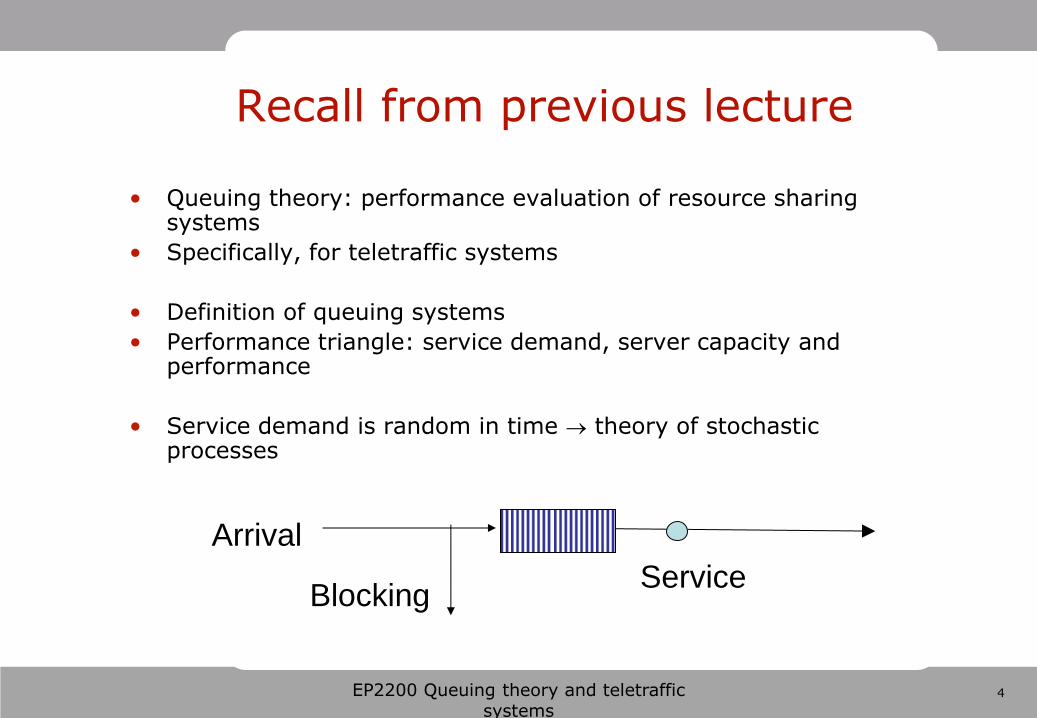
Recall from previous lecture

• Queuing theory: performance evaluation of resource sharing systems

• Specifically, for teletraffic systems

• Definition of queuing systems

• Performance triangle: service demand, server capacity and performance

• Service demand is random in time theory of stochastic processes

Service

Arrival

Blocking


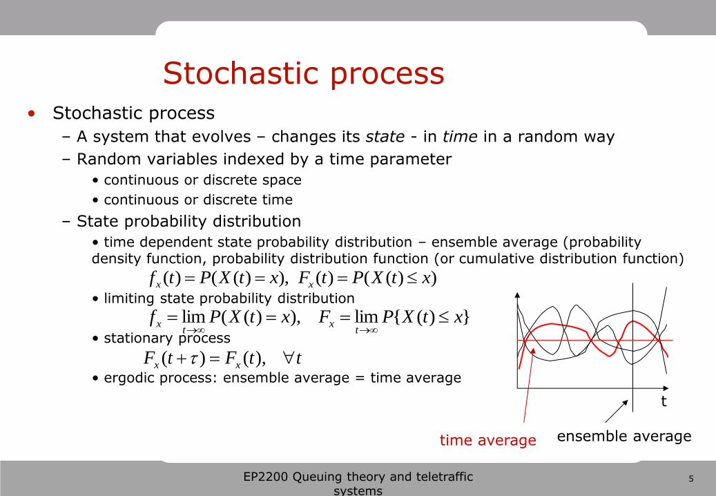
Stochastic process • Stochastic process

– A system that evolves – changes its state - in time in a random way

– Random variables indexed by a time parameter

• continuous or discrete space

• continuous or discrete time

– State probability distribution

• time dependent state probability distribution – ensemble average (probability density function, probability distribution function (or cumulative distribution function)

• limiting state probability distribution

• stationary process

• ergodic process: ensemble average = time average

ensemble average time average

t

))(()(),)(()( xtXPtFxtXPtf xx

})({lim),)((lim xtXPFxtXPft

xt

x

ttFtF xx ),()(


Outline for today





–continuous-time Markov-chains

• Graph and matrix representation

• Transient and stationary state of the process

7

Poisson process

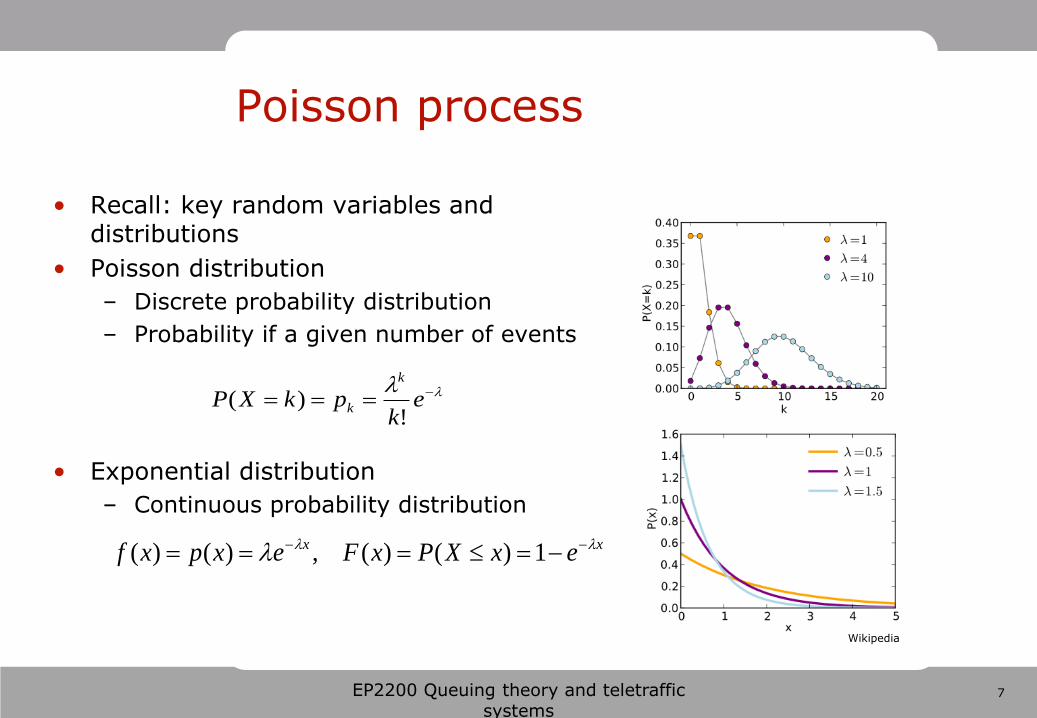
• Recall: key random variables and distributions

• Poisson distribution

– Discrete probability distribution

– Probability if a given number of events

• Exponential distribution

– Continuous probability distribution

EP2200 Queuing theory and teletraffic systems

ek

pkXPk

k!

)(

xx exXPxFexpxf 1)()(,)()(

Wikipedia


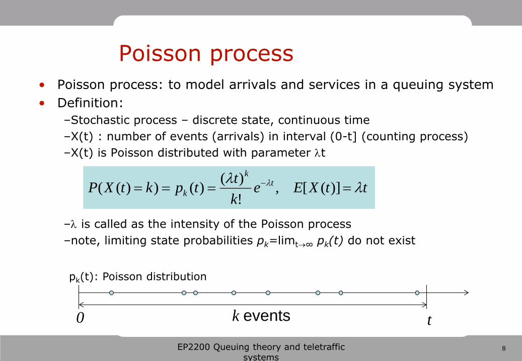
Poisson process

• Poisson process: to model arrivals and services in a queuing system

• Definition:

–Stochastic process – discrete state, continuous time

–X(t) : number of events (arrivals) in interval (0-t] (counting process)

–X(t) is Poisson distributed with parameter t

– is called as the intensity of the Poisson process

–note, limiting state probabilities pk=limt∞ pk(t) do not exist

pk(t): Poisson distribution

0 t k events

ttXEek

ttpktXP t

k

k )]([,

!

)()())((


• Def: The number of arrivals in period (0,t] has Poisson distribution with parameter t, that is:

• Theorem: For a Poisson process, the time between arrivals (interarrival time) is exponentially distributed with parameter :

– Recall exponential distribution:

– Proof:

tet)Pt)PtP 1 until arrival no(1 until arrival oneleast at ()(

Poisson process

tk

k ek

ttpktXP

!

)()())((

number of arrivals

Poisson distribution

interarrival time

exponential

pk(t): Poisson distribution

0 t k events

Exp()

1][,1)()(,)( EetPtFetf tt


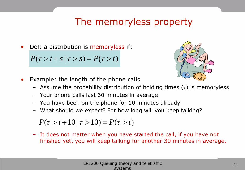
• Def: a distribution is memoryless if:

• Example: the length of the phone calls

– Assume the probability distribution of holding times () is memoryless

– Your phone calls last 30 minutes in average

– You have been on the phone for 10 minutes already

– What should we expect? For how long will you keep talking?

– It does not matter when you have started the call, if you have not finished yet, you will keep talking for another 30 minutes in average.

The memoryless property

)()|( tPsstP

)()10|10( tPtP


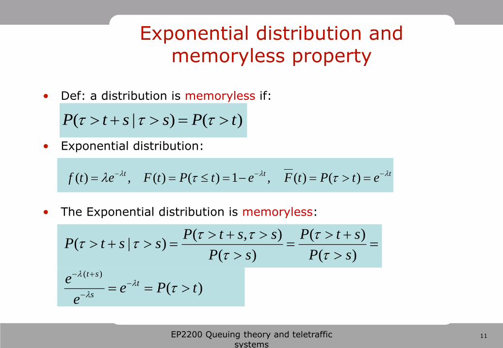
• Def: a distribution is memoryless if:

• Exponential distribution:

• The Exponential distribution is memoryless:

Exponential distribution and memoryless property

ttt etPtFetPtFetf )()(,1)()(,)(

)()|( tPsstP

)(

)(

)(

)(

),()|(

)(

tPee

e

sP

stP

sP

sstPsstP

t

s

st

12

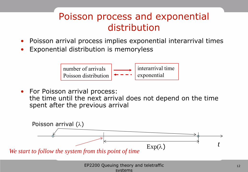
• Poisson arrival process implies exponential interarrival times

• Exponential distribution is memoryless

• For Poisson arrival process: the time until the next arrival does not depend on the time spent after the previous arrival

Poisson process and exponential distribution

number of arrivals

Poisson distribution

interarrival time

exponential

We start to follow the system from this point of time

EP2200 Queuing theory and teletraffic systems

Poisson arrival ()

Exp() t


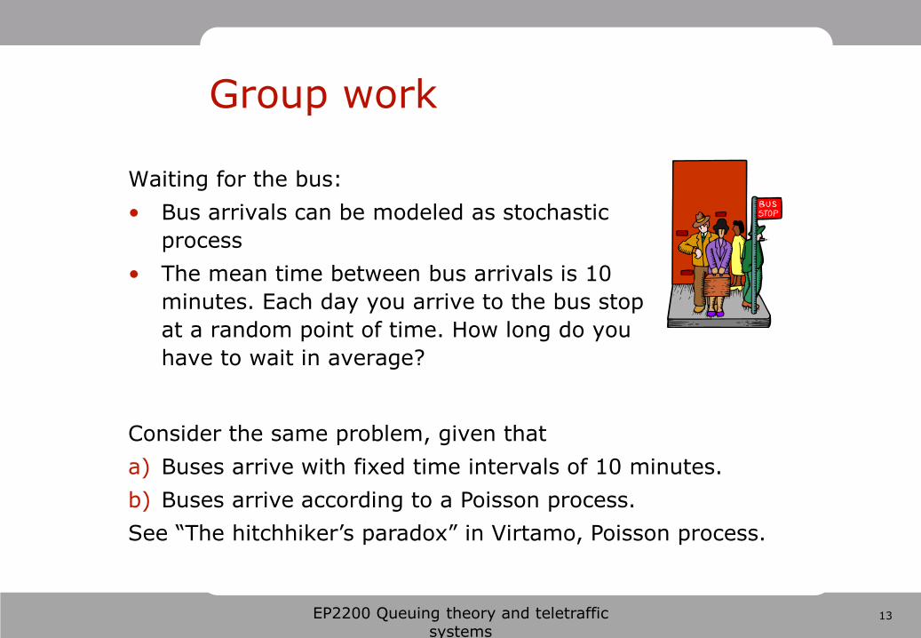
Group work

Waiting for the bus:

• Bus arrivals can be modeled as stochastic

process

• The mean time between bus arrivals is 10

minutes. Each day you arrive to the bus stop

at a random point of time. How long do you

have to wait in average?

Consider the same problem, given that

a) Buses arrive with fixed time intervals of 10 minutes.

b) Buses arrive according to a Poisson process.

See “The hitchhiker’s paradox” in Virtamo, Poisson process.


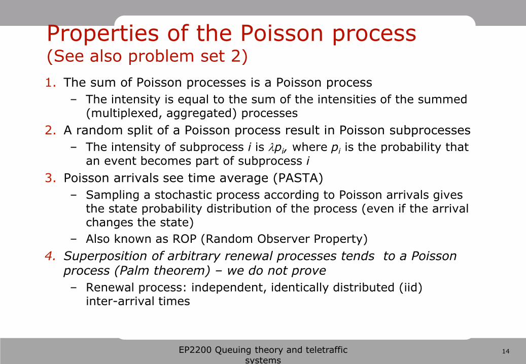
1. The sum of Poisson processes is a Poisson process

– The intensity is equal to the sum of the intensities of the summed (multiplexed, aggregated) processes

2. A random split of a Poisson process result in Poisson subprocesses

– The intensity of subprocess i is pi, where pi is the probability that an event becomes part of subprocess i

3. Poisson arrivals see time average (PASTA)

– Sampling a stochastic process according to Poisson arrivals gives the state probability distribution of the process (even if the arrival changes the state)

– Also known as ROP (Random Observer Property)

4. Superposition of arbitrary renewal processes tends to a Poisson process (Palm theorem) – we do not prove

– Renewal process: independent, identically distributed (iid) inter-arrival times

Properties of the Poisson process (See also problem set 2)


Outline for today





– Continuous-time Markov-chains

– Graph and matrix representation

– Transient and stationary state of the process


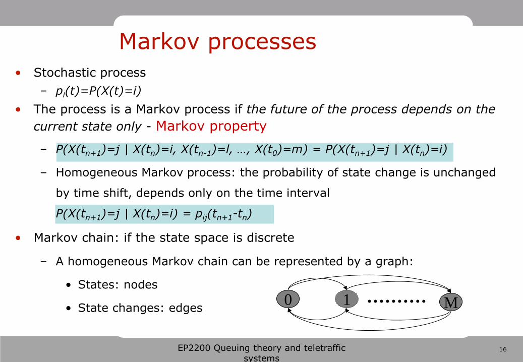
Markov processes

• Stochastic process

– pi(t)=P(X(t)=i)

• The process is a Markov process if the future of the process depends on the

current state only - Markov property

– P(X(tn+1)=j | X(tn)=i, X(tn-1)=l, …, X(t0)=m) = P(X(tn+1)=j | X(tn)=i)

– Homogeneous Markov process: the probability of state change is unchanged

by time shift, depends only on the time interval

P(X(tn+1)=j | X(tn)=i) = pij(tn+1-tn)

• Markov chain: if the state space is discrete

– A homogeneous Markov chain can be represented by a graph:

• States: nodes

• State changes: edges 1 0 M

17 2G1318 Queuing theory and teletraffic systems

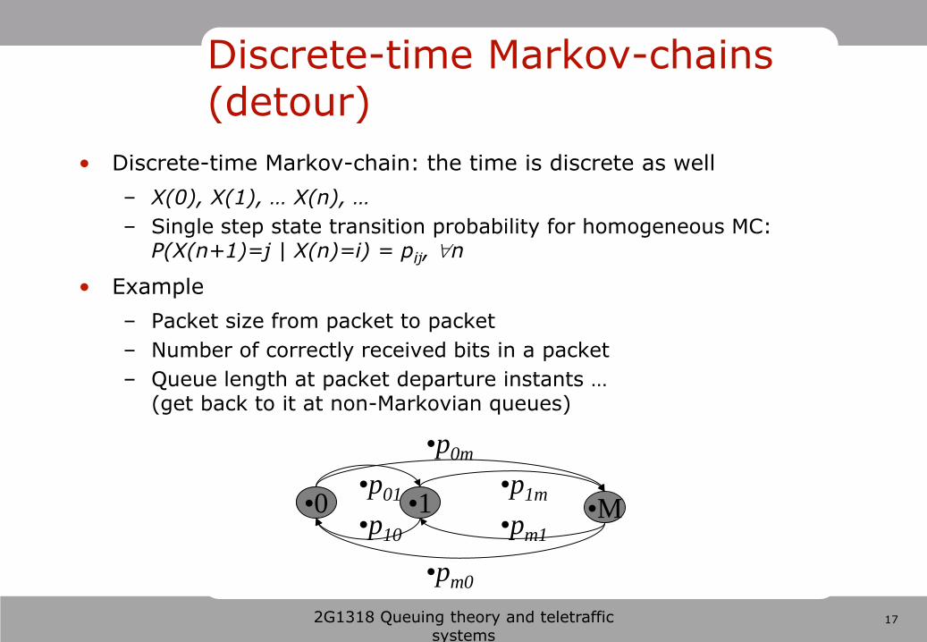
Discrete-time Markov-chains (detour)

• Discrete-time Markov-chain: the time is discrete as well

– X(0), X(1), … X(n), …

– Single step state transition probability for homogeneous MC: P(X(n+1)=j | X(n)=i) = pij, n

• Example

– Packet size from packet to packet

– Number of correctly received bits in a packet

– Queue length at packet departure instants … (get back to it at non-Markovian queues)

•1 •0 •M •pm1

•p01

•pm0

•p1m

•p0m

•p10


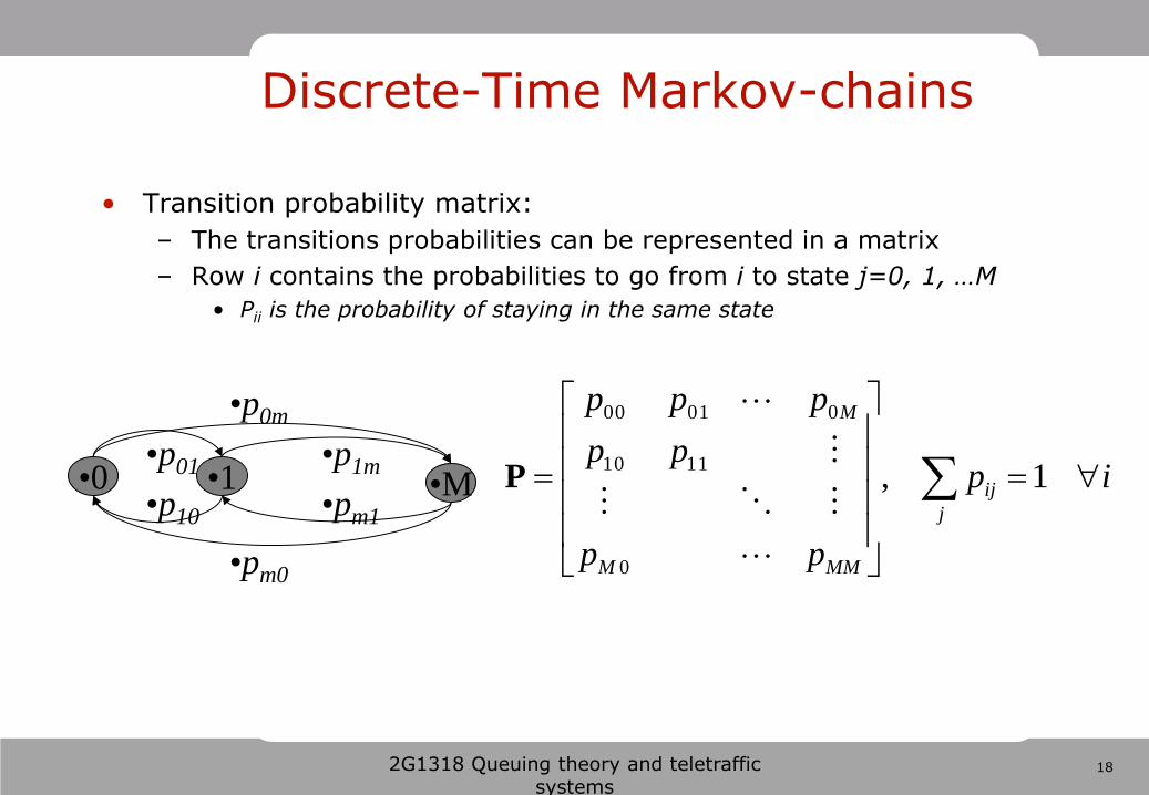
• Transition probability matrix:

– The transitions probabilities can be represented in a matrix

– Row i contains the probabilities to go from i to state j=0, 1, …M

• Pii is the probability of staying in the same state

ip

pp

pp

ppp

j

ij

MMM

M

1,

0

1110

00100

P

Discrete-Time Markov-chains

•1 •0 •M •pm1

•p01

•pm0

•p1m

•p0m

•p10


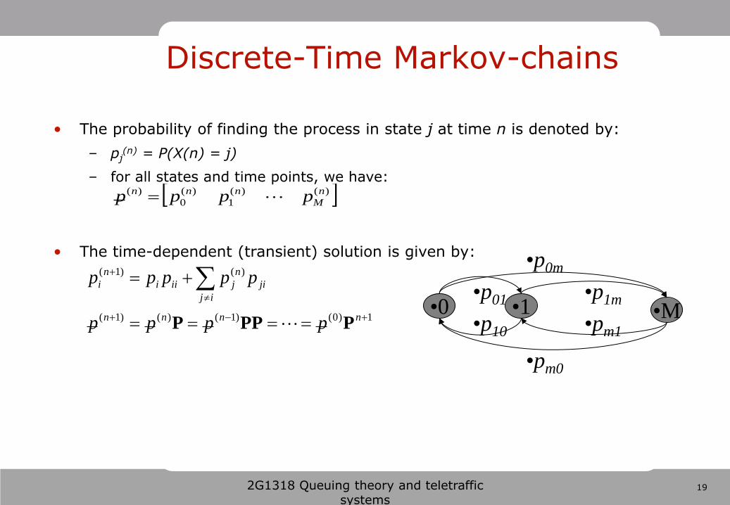
• The probability of finding the process in state j at time n is denoted by:

– pj(n) = P(X(n) = j)

– for all states and time points, we have:

• The time-dependent (transient) solution is given by:

)()(

1

)(

0

)( n

M

nnn pppp

1)0()1()()1(

)()1(

nnnn

ji

ij

n

jiii

n

i

pppp

ppppp

PPPP


•1 •0 •M •pm1

•p01

•pm0

•p1m

•p0m

•p10

20

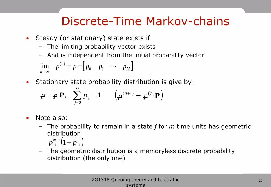
• Steady (or stationary) state exists if

– The limiting probability vector exists

– And is independent from the initial probability vector

• Stationary state probability distribution is give by:

• Note also:

– The probability to remain in a state j for m time units has geometric distribution

– The geometric distribution is a memoryless discrete probability distribution (the only one)

2G1318 Queuing theory and teletraffic systems

M

n

nppppp 10

)(lim

1,0

M

j

jppp P

jj

m

jj pp 11

P)()1( nn pp



Continuous-time Markov chains (homogeneous case)

• Continuous time, discrete space stochastic process, with Markov property, that is:

• State transition can happen in any point of time

• Example:

– number of packets waiting at the output buffer of a router

– number of customers waiting in a bank

• The time spent in a state has to be exponential to ensure Markov property:

– the probability of moving from state i to state j sometime between tn and tn+1 does not depend on the time the process already spent in state i before tn.

1101

011

),)(|)((

))(,)(,)(|)((

nnnn

nnn

ttttitXjtXP

mtXltXitXjtXP

t0 t1 t2 t3 t4 t5

sta

tes


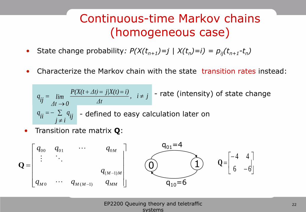
Continuous-time Markov chains (homogeneous case)

• State change probability: P(X(tn+1)=j | X(tn)=i) = pij(tn+1-tn)

• Characterize the Markov chain with the state transition rates instead:

ijij

qii

q

ji,Δt

i)j|X(t)Δt)P(X(tlim

0Δtij

q

• Transition rate matrix Q:

MMMMM

MM

M

qqq

q

qqq

)1(0

)1(

00100

Q

- rate (intensity) of state change

- defined to easy calculation later on

0 1

q01=4

q10=6

66

44Q


Summary

• Poisson process:

– number of events in a time interval has Poisson distribution

– time intervals between events has exponential distribution

– The exponential distribution is memoryless

• Markov process:

– stochastic process

– future depends on the present state only, the Markov property

• Continuous-time Markov-chains (CTMC)

– state transition intensity matrix

• Next lecture

– CTMC transient and stationary solution

– global and local balance equations

– birth-death process and revisit Poisson process

– Markov chains and queuing systems

– discrete time Markov chains

poisson process markov process - kth · poisson process • poisson process: to model arrivals and...

Documents