plantgl: a python-based geometric library for 3d plant modelling at

HAL Id: inria-00191126https://hal.inria.fr/inria-00191126v3

Submitted on 27 Nov 2007

HAL is a multi-disciplinary open accessarchive for the deposit and dissemination of sci-entific research documents, whether they are pub-lished or not. The documents may come fromteaching and research institutions in France orabroad, or from public or private research centers.

L’archive ouverte pluridisciplinaire HAL, estdestinée au dépôt et à la diffusion de documentsscientifiques de niveau recherche, publiés ou non,émanant des établissements d’enseignement et derecherche français ou étrangers, des laboratoirespublics ou privés.

PlantGL : a Python-based geometric library for 3D plantmodelling at different scales

Christophe Pradal, Frédéric Boudon, Christophe Nouguier, Jérôme Chopard,Christophe Godin

To cite this version:Christophe Pradal, Frédéric Boudon, Christophe Nouguier, Jérôme Chopard, Christophe Godin.PlantGL : a Python-based geometric library for 3D plant modelling at different scales. [ResearchReport] RR-6367, INRIA. 2007. <inria-00191126v3>

https://hal.inria.fr/inria-00191126v3

https://hal.archives-ouvertes.fr

appor t de r ech er ch e

ISS

N02

49-6

399

ISR

NIN

RIA

/RR

--63

67--

FR+E

NG

Thème BIO

INSTITUT NATIONAL DE RECHERCHE EN INFORMATIQUE ET EN AUTOMATIQUE

PlantGL: a Python-based geometric library for 3Dplant modelling at different scales

Christophe Pradal — Frederic Boudon — Christophe Nouguier — Jérôme Chopard —Christophe Godin

N° 6367

Novembre 2007

Centre de recherche INRIA Sophia Antipolis – Méditerranée2004, route des Lucioles, BP 93, 06902 Sophia Antipolis Cedex (France)

Téléphone : +33 4 92 38 77 77 — Télécopie : +33 4 92 38 77 65

PlantGL: a Python-based geometric library for3D plant modelling at different scales

Christophe Pradal ∗ , Frederic Boudon ∗ , Christophe Nouguier ,Jerome Chopard , Christophe Godin

Theme BIO — Systemes biologiquesEquipes-Projets VirtualPlants

Rapport de recherche n° 6367 — Novembre 2007 — 39 pages

Abstract: In this paper, we present PlantGL, an open-source graphic toolkitfor the creation, simulation and analysis of 3D virtual plants. This C++ geo-metric library is embedded in the Python language which makes it a powerfuluser-interactive platform for plant modelling in various biological applicationdomains.

PlantGL makes it possible to build and manipulate geometric models ofplants or plant parts, ranging from tissues and organs to plant populations.Based on a scene graph augmented with primitives dedicated to plant represen-tation, several methods are provided to create plant architectures from eitherfield measurements or procedural algorithms. Because they reveal particularlyuseful in plant design and analysis, special attention has been paid to the defi-nition and use of branching system envelopes. Several examples from differentmodelling applications illustrate how PlantGL can be used to construct, analyseor manipulate geometric models at different scales.

Key-words: software architecture, surfacic geometry, virtual plants, plantarchitecture, crown envelops, canopy reconstruction, scene graph

∗ These two authors contributed equally to the paper

PlantGL : une bibliotheque geometrique enPython pour la modelisation 3D des plantes a

differentes echelles

Resume : Dans cet article, nous presentons PlantGL, une bibliothequegraphique libre pour la creation, la simulation et l’analyse de plantes virtuelles3D. Cette bibliotheque geometrique ecrite en C++ est accessible depuis le languagePython. Elle constitue la base d’une plateforme interactive pour la modelisationdes plantes dans plusieurs domaines applicatifs de la biologie.

PlantGL permet de construire et de manipuler des modeles geometriques deplantes a differentes echelles, depuis les tissus cellulaires et les organes jusqu’auxpopulations de plantes. Plusieurs methodes sont proposees pour generer desarchitectures de plantes a partir de donnees mesurees sur le terrain ou demethodes procedurales. Ces methodes s’appuient sur une structure de graphede scene augmentee de primitives geometriques adaptees a la representation deplantes. Du fait de leur importance pour le design et l’analyse de plante, uneattention particuliere a ete apportee a la definition et a l’utilisation d’enveloppespour representer des systemes ramifies . Plusieurs exemples applicatifs illustrentcomment PlantGL peut etre utilisee pour construire, analyser et manipuler desmodeles geometrique de plantes a differentes echelles.

Mots-cles : architecture logicielle, geometrie surfacique, plantes virtuelles,architecture des plantes, enveloppes de houppiers, reconstruction de canopees,graphe de scene

The PlantGL library 3

1 Introduction

The representation of plant forms in computer scenes has for long been rec-ognized as a difficult problem in computer graphics applications. In the lasttwo decades, several algorithms and software platforms have been proposedto solve this problem with a continuously improving level of efficiency, e.g.[1, 2, 3, 4, 5, 6, 7, 8]. Due to the increasing use of computer models in bi-ological research, the design of 3D geometric models of plants has also be-come an important aspect of various biological applications in plant science,e.g. [9, 10, 11, 12, 13, 14, 15]. These applications raise specific problems thatderive from the need to represent plants with a botanical or geometric accuracyat different scales, from tissues to plant communities. However, in comparisonwith computer graphics applications, less effort has been devoted to the develop-ment of geometric modelling systems adapted to the requirements of biologicalapplications.

In this context, the most successful and widespread plant modelling systemhas been developed by P. Prusinkiewicz and his team since the late 80’s at theinterface between biology and computer graphics. They designed a computerplatform, known as L-Studio/VLab, for the simulation of plant growth basedon L-systems [16, 1]. This system makes it possible to model the development ofplants with efficiency and flexibility as a process of bracketed-string rewriting.In a recent version of LStudio/VLab, Karwowski and Prusinkiewicz changed theoriginal cpfg language for a compiled language, L+C, built on the top of theC++ programming language. The resulting gain of expressiveness facilitatesthe specification of complex plant models in L+C [18]. An alternative imple-mentation of a L-system-based software for plant modeling was designed by W.Kurth [19] in the context of forestry applications. This simulation system, calledGroGra, was also recently re-engineered in order to model the development ofobjects more complex than bracketed strings. The resulting simulation system,GroIMP, is an open-source software that extends the chain rewriting principleof L-Systems to general graph rewriting with relational graph growth (RGG),[20, 21]. Similarly to L+C, this system has been defined on the top of a widelyused programming language (here Java). Non-language oriented platforms werealso developed. One of the first ones was designed by the AMAP group. TheAMAP software [2, 22] makes it possible to build plants by tuning the parame-ters of a predefined, hard-coded, model. Geometric symbols for flowers, leaves,fruits, etc., are defined in a symbol library and can be modified or created withspecific editors developed by AMAP. In this framework, a wide set of parameter-files has been designed corresponding to various plant species. In the context ofapplications more oriented toward computer graphics, the XFrog software [4, 23]is a popular example of a plant simulation system dedicated to the intuitive de-sign of plant geometric models. In XFrog, components representing basic plantorgans like leaves, spines, flowerlets or branches can be multiplied in space usinghigh-level multiplier components. Plants are thus defined as graphs representingseries of multiplication operations. The XFrog system provides an easy to use,intuitive system to design plant models, with little biological expertise needed.

Therefore, if accuracy, conciseness and transparency of the modeling processis required, object-oriented, rule-based platforms, such as L-studio/VLab orGroIMP, are good candidates for modelers. If interactive and intuitive modeldesign is required, with little biological expertise, then component-based or

RR n° 6367

4 C. Pradal, F. Boudon, C. Nouguier, J. Chopard & C. Godin

sketch-based systems like XFrog are the best candidates. However, if easinessto explore and mathematically analyse plant scenes is required, none of theabove approaches is completely satisfactory. Such an operation requires high-level user interaction with plant scenes and dedicated high-level mathematicalprimitives. In this aim, our team developed several years ago the AMAPmodsoftware [24], and its most recent version, VPlants, which enables modelers tocreate, explore and analyse plant architecture databases using a powerful scriptlanguage. In a way complementary to L-Studio/VLab, VPlants allows theuser to efficiently analyse plant architecture databases and scenes from manyexploratory perspectives in a language-based, interactive, manner [25, 26, 27,28]. The PlantGL library was developed to support geometric processing onplant scenes in VPlants, for applications ranging from computer graphics [29, 30]to different areas of biological modeling [31, 32, 33, 14, 34, 35]. A number of high-level requirements were imposed by this context. Similarly to AMAPmod/VPlants,the library should be open-source, it should be fully compatible with the datastructure used in AMAPmod/VPlants to represent plants, i.e. multi-scale treegraphs (MTGs), it should be accessible through an efficient script language tofavor interactive exploration of plant databases, it should be easy to use forbiologists or modellers and should not impose a particular modelling approach,it should be easily extended by users to progressively adapt to the great varietyof plant modelling applications, and finally, it should be interoperable with othermain plant modelling platforms.

These main requirements lead us to integrate a number of new and originalfeatures in PlantGL that makes it particularly adapted to plant modelling. Itis based on the script language Python, which enables the user to manipulategeometric models interactively and incrementally, without compiling the scenecode or recomputing the entire scene after each scene modification. The embed-ding in Python is critical for a number of additional reasons: i) the modeller hasaccess to a powerful object-oriented language for the design of geometric scenes,ii) the language is independent of any underlying modelling paradigm and allowsthe definition of new procedural models, iii) high-level manipulations of plantscenes provide users the ease to concentrate on application issues rather than ontechnical details, iv) the large set of available Python scientific packages can befreely and easily accessed by modelers in their applications. From its contentsperspective, PlantGL provides a set of geometric primitives for plant modellingthat can be combined in scene-graphs dedicated to multiscale plant represen-tation. New primitives were developed to address biological questions at eithermacroscopic or microscopic scales. At plant scale, envelope-based primitiveshave been designed to model plant crowns as volumetric objects. At cell scale,tissue objects representing arrangements of plant cells enable users to model thedevelopment of plant tissues such as meristems. Particular attention has beenpaid to the design of the library to achieve a high-level of reuse and extensibility(e.g. data structures, algorithms and GUIs are clearly separated). To favor theexchange of models and databases between users, PlantGL can communicatewith other modelling platforms such as LStudio/VLab and is available under anopen-source license.

In this paper, we present the PlantGL geometric library and its applicationto plant modelling. Section 2 describes the design principles and rationales thatunderly the library architecture. It also briefly introduces the main scene graphstructure and the different library objects: geometric models, transformations,

INRIA


algorithms and visualization components. Then, a detailed description of thegeometric models and methods dedicated to the construction of plant scenes isprovided in section 3. This includes the modeling of organs, crowns, foliage,branching systems and plant tissues. A final section illustrates how PlantGLcomponents can be used and assembled to answer particular questions fromcomputer graphics or biological applications at different levels of a modellingapproach: creating, analysing, simulating and assessing plant models.

2 PlantGL design and implementation

A number of high-level goals have guided the design and development of PlantGLto optimize its reusability and diffusion:

• Usefulness : PlantGL is primarily dedicated to researchers in the plantmodelling community who do not necessarily have any a priori knowledgein computer graphics. Its interface with modellers and end-users shouldbe intuitive with a short learning curve.

• Genericity : PlantGL should not impose a particular modelling paradigmon users. Rather, it should allow them to design their own approach in apowerful way.

• Quality : Quality is a major aspect of software diffusion and reusability.PlantGL should therefore be developed with software quality guarantees.

• Interoperability : PlantGL should also be interoperable with various plantmodelling systems (e.g. L-studio/VLab, AMAP, etc.) and graphic toolkits(e.g. Pov-Ray, Vrml, Blender, etc.).

• Portability : PlantGL should be available on major operating systems (e.g.Linux, Microsoft Windows, MacOSX).

In this section we detail how these requirements have been translated intochoices at different levels of the system design.

2.1 Software architecture

The system architecture derives from a set of key design choices:

• Open-source : PlantGL is an open-source software that may be freely usedand extended.

• Script-language based system : PlantGL is built on the top of the powerfulscript language, Python. The use of a script language allows users to havea high level of computational interaction with their models.

• Software engineering : Object-oriented design is useful to organize largecomputational projects and enhance code reuse. However, designing reusableand flexible software remains a difficult task. We addressed this problemby using advanced software engineering tools such as design patterns [36].

RR n° 6367


• Modularity : PlantGL is composed of several independent modules like ageometric library, GUI components and Python wrappers. They can beused alone or combined within a specific application.

• Hybrid System : Core computational components of PlantGL are imple-mented in the C++ compiled language for performance. However, for flexi-bility of use, these components are also exported in the Python language.

Among all the script available languages, Python was found to present aunique compromise between the following features:

• Python is an open-source software;

• it is available on the main operating systems;

• it is a powerful object-oriented language;

• it is simple to use and its syntax is sufficiently intuitive for non-computerscientists (e.g. for biologists);

• it is fully compatible with C++;

• the Python community is large and very active;

• a large number of other scientific libraries are available and can be im-ported in the language at any time of a model development.

The overall architecture layout of PlantGL is shown in Figure 1, includingseveral layers of encapsulation and abstraction. The geometric library and theGUI lie in the core of PlantGL. The geometric library encapsulates a scene-graphdata structure, a taxonomy of geometric objects and a set of algorithms (forinstance for OpenGL rendering). The GUI is developed as a set of Qt widgets andcan be combined with previous components to provides visualization facilities.On top of this first layer, a set of wrappers create interfaces of the C++ classes intothe Python language. All these interfaces are gathered into a Python modulenamed PlantGL. This module is integrated seamlessly with standard Pythonand thus enables further abstraction layers, written in Python. Extension ofthe library can be done using either C++ or Python.

2.2 Basic components

The basic components of PlantGL are scene-graphs that contain scene objects(geometry, appearance, transformation, etc.), actions that define algorithmsthat can be applied to scene-graphs, and the visualization tools.

2.2.1 Scene-graphs

Scene-graphs are a common data structure used in computer graphics to modelscenes [37]. They provide both a high-level view of the application’s data aswell as a mechanism to perform the low-level computations necessary to drivea rendering pipeline such as OpenGL. Basically, a scene-graph is a directed,acyclic graph (DAG), whose nodes hold the information about the elements thatcompose the scene. In a DAG, nodes may have more than one parent, which

INRIA


Figure 1: Layout of the PlantGL architecture. It contains three main compo-nents: a geometric library, a GUI and Wrappers. The two first components arewritten in C++ for efficiency. PlantGL primitives can be used by modellers todevelop scripts, procedures and applications in the embedding language Python.Data structures can be imported from and exported to other plant modellingsoftwares

enables parent nodes to share child nodes within the graph via the instantiationmechanism.

In PlantGL, an object-oriented version of scene-graphs was implemented tofacilitate the customization of scene-graph node processing. Scene-graphs aremade of nodes of different types. Types may be one of geometry, appearance,shape, transformation, and group. Scene-graph nodes are organized as a DAGhierarchy. Terminal nodes contain shapes pointing to both a geometry node(which contains a geometric model, see section 2.2.2) and an appearance node(e.g. which defines a color, a material or a texture). Non terminal nodes cor-respond to group or transformation nodes (see section 2.2.3). They are used tobuild complex objects from simple geometric models.

2.2.2 Geometric models

Two families of geometric models are available in the library: Explicit andParametric models. Explicit models are defined as sets of discrete primitiveslike points, lines or polygons that can be directly drawn by graphics cards. Theyenable to express geometric models in a generic but low level way and are thuscomplex to manipulate. On the opposite, parametric models are defined usingequations that involve one or several parameters. Parametric models offer ahigher level of abstraction and are thus simpler to manipulate. However, tobe displayed, parametric models have to be transformed into an explicit repre-sentation. This is done by discretizing algorithms defined for each parametricmodel. The discretization process is controlled by parameters indicating howmany primitives have to be created.

PlantGL contains a number of geometric models to represent 3D points,curves, surfaces and volumes. Curves include Polyline, Bezier and NURBS .They are used for instance to generate surfaces or to represent the medial axis of

RR n° 6367


an object. Surfaces and volumes may be represented by PolygonMesh, surfacesof revolution (SOR), Patch, Extrusion and Hull . SOR include simple shapes(sphere, cylinder, frustum, paraboloid) and more generic ones like Revolution(revolution of a curve along an axis). Patch surfaces include Bezier , NURBS ,and ElevationGrid surfaces used for terrain modelling. Extrusion (or generalizedcylinder) is a sweep surface useful for the modelling of branches. Hulls are 3Denvelopes that may be used to model tree crowns.

2.2.3 Transformations and compositions

Transformed nodes allow the user to define the position, orientation and sizeof a geometric object. They contain classical translation, rotation and scalingnodes. Rotations may be specified in various forms (via matrices, Euler an-gles,...). A particular transformation named Taper proposes a gradual scalingof subsequent perpendicular planes to a given direction. This non-affine trans-formation enables the modeller to transform a cylinder into a truncated coneand is generally used in the representation of branch segments. Transformednodes embed a shape on which the transformation is applied.

A Group node, or a composite node, defines a union of scene objects whichembeds a list of geometry nodes. Groups are mainly used to apply a giventransformation to a set of objects as a whole. A Group node may point to otherGroup nodes and define a subgraph of nodes.

2.2.4 Algorithms

In PlantGL, algorithms are separated from data structures for flexibility andmaintenance purpose. To be applied on a scene, some algorithms need totraverse the scene-graph structure. Scene-graph traversals are different fromstandard graph traversal since nodes are heterogeneous and need to be treatedaccording to their type. To achieve this efficiently, traversal processes are basedon double dispatch technique via the visitor design pattern [36]. This designpattern makes it possible to keep functions outside node objects by delegatingthe mapping from node to function to a separate visitor object called an action.The action holds all the algorithm functions for every types of nodes in thesystem. It is thus possible to add new algorithms by implementing new actionswithout modifying the node classes (see section 2.4). By splitting specificationand implementation, PlantGL scene-graph preserves flexibility without loosingperformances.

In the actual implementation, PlantGL supports approximatively 40 actions.The main ones can be classified into the following categories :

• Converter : Algorithms that convert geometries into explicit representa-tions (e.g. Discretizer or Tesselator actions), or into Bounding Boxes orWire.

• Renderer : OpenGL rendering for various modes: volumetric, skeleton,bounding box, etc.

• Import / Export : parser and exporter of various classical formats namelyPovRay, Vrml, etc. or to plant dedicated systems like AMAPmod/VPlants,LStudio/VLab, AMAPsim and VegeStar.

INRIA


• Fitting : Fitting algorithms have been integrated into the library. Facili-ties to compute convex hull [38], bounding volumes (sphere [39], box) canbe used to compute a global representation from a set of detailed shapes.

• Projection : Algorithm based on OpenGL to project 3D scenes onto 2Dplanes.

• Grids : Partitioning of the 3D space into multiscale grids such as Oc-tree. Detection of intersection between voxels and triangles of the sceneis carried out using the algorithm described in [40].

• Ray casting : Two versions of the algorithms are implemented. The firstone is CPU-based, and is implemented as C++ routines with grids usedto determine which shape to test for ray intersection. The second oneis GPU-based, and uses OpenGL picking feature to compute the differentshape interceptions of a small orthographic viewport, featuring a beam.

• Analysis : Algorithms that compute particular properties of the scene,like the total number of polygons, the surface or volume, the center or theinertia axes of the scene.

The use of these algorithms is illustrated in section 4 in the context of dif-ferent biological applications.

2.2.5 Visualization tools

The PlantGL Viewer (Figure 2) provides facilities to visualize scene-graphs. Dif-ferent types of rendering modes are available including volumetric, wire, skele-ton, and bounding box. Camera and lights positions and properties can beinteractively modified. Scene-graphs organization and node properties can beexplored with adapted widgets allowing to access to various pieces of informa-tion about the scene, like the number, volume, surface or bounding box of thescene elements. Simple edition features (such as a shape material editor) areavailable. Screen-shots can be easily made and exported in documents or as-sembled into movies. Most of the viewer features can be set using buttons orcontext menus and are also available with procedure call.

The viewer and the scene access are multi-threaded so that a user can stillinteract with the scene from a Python shell during visualization.

Several types of dialog boxes can also be interactively created in the Viewerfrom the Python shell. Results of the dialog is returned to the Python processusing multi-threaded communications (see section 2.4). This enables graphicalcontrol of a Python modelling process through the Viewer.

2.3 Creating scene-graphs

There are different ways for application developers to create and process a scene-graph depending both on performance constraints and their familiarity withcomputer graphics concepts.

• Declarative language. PlantGL provides a declarative language, GML, sim-ilar to VRML [41] with extensions for plant geometric objects. GML adds

RR n° 6367


Figure 2: Visualization of the detailed representation of a 15 years walnut tree[10] with the PlantGL viewer.

persistence capabilities to PlantGL in both ascii and binary versions. Ex-ternal applications can use this file format to describe a static scene andcall PlantGL as an external module to render it. The GML language isdescribed in [42].

• Scene-graph programming API. For C++ applications, it is possible to linkdirectly with the PlantGL library. In this case, PlantGL features can beextended by adding new objects and new actions.

• Interpreted language. The full PlantGL API is accessible from the Pythonlanguage. Combination of high level tools and language such as PlantGLand Python allows rapid prototyping of new models and applications [43].Moreover, numerous scientific modules for Python exist and can be reused[44].

PlantGL provides different ways for users and applications to create scenes.A scene can first be described in GML. The GML file can then be loaded andthe scene rendered. In such a case, the scene is static and the communication isone way. For performance and fast communication, a second solution consistsof creating the scene in C++ and link the application with the C++ PlantGLlibrary. Finally, for rapid developments, prototyping, and tests, a scene can becreated procedurally in Python.

2.4 Implementation issues

Different issues have to be addressed in order to implement an efficient scene-graph that preserves performances and flexibility. Literature on scene-graphs[45] offers various interesting solutions that were formalized as design patternsand which inspired our implementation.

Memory management - Scene-graphs have to deal with large numberof geometric elements. This is particularly true for natural scenes. Memoryconsumption is thus an issue. Repetitive structures such as trees enable massiveuse of instantiation. This technique, however, implies to reference several timesthe same object. Allocation and deallocation of this object in memory can thusbe problematic. To address this issue, we use Reference counting pointers [46]

INRIA


which manages pointers to dynamically allocated objects. They are responsiblefor automatic deletion of the objects when no longer needed.

Double dispatch - As stated in section 2.2.4, scene-graph traversal imple-ments a double-dispatch technique via the visitor design pattern. With such anapproach, algorithms can be added without any modification of the hierarchyof objects. However, at runtime, matching a particular data structure to itsappropriate algorithms is not a trivial task. Each node of the scene-graph hasan apply method that takes an action object as an argument. The node makesa call to the action, passing itself as an argument, and the action executes itsalgorithm depending on the actual node type. Thus, the visitor design patternsimulates a double-dispatch in C++, which is a single-dispatch object orientedlanguage.

Wrappers - The seamless transition between C++ and Python is ensuredby the Boost.Python library [47]. In contrast with concurrent tools, the in-teraction between C++ and Python is encoded explicitly in C++. This wrappingcode is then compiled into a dynamic library, usable as a Python module. Onone hand, Boost.Python maps C++ classes and their interfaces to correspondingPython classes. On the other hand, it transparently converts Python objectsback to C++ pointers or references, thus providing dynamic, run-time depen-dent interaction between C++ based objects. Since Boost.Python is based onadvanced meta-programming techniques, the code wrapping mainly consists ofsimple declaration of entry points in the library and is automatically translatedinto conversion functions.

Graphic performances -Plant geometry generally rely on important ver-tex set. In order to minimize time cost for sending all the vertex to the GPU,the vertex are packed into arrays that can be sent in one command to the card.Moreover, OpenGL command for drawing shapes instantiated multiple times arepacked into display lists that can be reused efficiently when needed.

Multi-threading - Viewer and shell processing are done in separated threads.For this, Qt threads implementation were used. Inter-threads communication ismade using Qt event dispatch mechanism which is extended with synchronizeddispatch using mutex.

3 Construction of Plant Models

3.1 Plant organs

As stated in section 2.2.2, a taxonomy of geometric models is implementedin PlantGL. During implementation, we focused on models useful for naturalscene modelling and rendering. For instance, PlantGL contains thus cylindersand frustums to represent inter-nodes, Bezier and NURBS patches to modelcomplex organs such as leaves or flowers and generalized cylinders for branchesand stems.

During the creation of a scene-graph, complex objects can be modeled usingcomposition and instantiation. Simple procedures can be written in Python thatposition predefined symbols, for instance petals or leaves, using Transformationand Group objects, to create more complex objects by composition (Figure 3).Python, as a modelling language, allows the modeller to express a full range ofmodelling techniques. For instance, the pine cone (Figure 3.c) is built by placing

RR n° 6367


its scale using the golden angle. The following code sketches the placement ofeach scales. Size of successive scales in the spiral follows a logarithmic laws inthis case.from PlantGL import ∗sc = Scene ( )

de l taAngle = pi /(1+ sq r t ( 5 ) ) # the golden ang lede f distToTrunk (u ) : # with u in [ 0 , 2 ] , u < 1 f o r the bottom part

i f i < 1 : r e turn MaxDist∗ue l s e : r e turn MaxDist∗((2−u )∗∗2)

de f s i z e S c a l e (u ) :i f i < 1 : r e turn MaxSize∗ l og (1+u , 2 )e l s e : r e turn MaxDist∗ l og (3−u , 2 )

f o r i in range ( nbScale ) :s += AxisRotated ( ( 0 , 0 , 1 ) , i ∗deltaAngle ,

Trans lated ( ( distToTrunk (2∗ i / nbScale ) , 0 , i ) ,Sca led ( s i z e S c a l e (2∗ i / nbScale ) , smb ) )

(a) (b) (c)

Figure 3: (a) a tulip, (b) a cactus and (c) a pine cone. Models were createdwith simple Python procedure that create and position organs, like petal andleaves.

3.2 Crown models

3.2.1 Envelopes

Tree crown envelopes are used in different contexts like studying plant interac-tion with its environment (i.e. radiative transfers in canopies [9] or competitionfor space [48]), 3D tree model reconstruction from photographs [6], and interac-tive rendering [49]. They are one original key issue of PlantGL. In this section,we describe in detail three specific envelope models that were specifically de-signed to represent plant volumes: asymmetric, extruded and skinned hulls.

Asymmetric Hull - This envelope model, originally proposed by Horn[50] and Koop [51], then extended by Cescatti [9], makes it possible to defineasymmetric crown shapes based on ellipsoidal shapes.

The envelope is defined by six control points and two shape factors CT andCB (see Figure 4). The two first control point, PT and PB , respectively representtop and base points of the crown. The four other points P1 to P4 representthe different radius of the crown in four orthogonal directions. P1 and P3 areconstrained to lie in the xz plane and P2 and P4 in yz plane. These points define

INRIA


Figure 4: Asymmetric hull parameters.

a peripheral line L at biggest width of the crown when projecting it into thehorizontal plane. The projection of L in the horizontal plane is composed of fourellipse quarters centered on (0, 0). The height of the points of L is defined as aninterpolation of the heights of the control points. To be continuous at the controlpoints, we used factors cos2 θ and sin2 θ. Thus, a point Pθ,i,j of a quarter of Lbetween control points Pi and Pj with i, j ∈ [(1, 2), (2, 3), (3, 4), (4, 1)], locatedat an angle θ ∈

[0, π

2

), is defined as

Pθ,i,j =[rPi

cos θ, rPjsinθ, zPi

cos2 θ + zPjsin2 θ

]. (1)

The two shape factors CT and CB describe the curvature of the crown aboveand below the peripheral line. Points of L are connected to the top and basepoints with quarters of super-ellipse respectively of degrees CT and CB . LetPl ∈ L and PT be the top point of the envelope, the above super-ellipse quarterconnecting Pl and PT is defined as

P = (θ, r, z)| (r − rpT)CT

(rPl− rpT

)CT+

(z − zpT)CT

(zPl− zpT

)CT= 1

. (2)

Equivalent equation is obtained for below super-ellipse quarter using PB andCB instead of PT and CT .

Figure 5: Example of asymmetric hulls showing plasticity of this model torepresent tree crowns (inspired from Cescatti [9]).

Different shape factor values generate conical (Ci = 1), ellipsoidal (Ci = 2),concave (Ci ∈]0, 1[), or convex (Ci ∈]1,∞[)shapes. A great variety of shapes canbe achieved by modifying shape factor values (see Figure 5). Cescatti proposes

RR n° 6367


a simple methodology to measure the six control points and estimate the shapefactors directly in the field. In PlantGL, a graphic editor has been implementedwhich makes it possible to build envelopes from photographs or drawings. Forthis, reference images can be displayed in the background of the different editionviews. An illustration of this shape usage can be found for the interactive designof bonsai tree [29].

Extruded Hull - This model of extruded envelope was originally proposedby Birnbaum [52]. Such an envelope is built from a vertical and an horizontalprofile, respectively in the xz plane and in the xy plane. To build the envelope,the horizontal profile is swept inside the vertical profile.

For this, the vertical profile V is virtually split into slices by planes passingthrough equidistant points from the top (or by horizontal planes). These slicesare used to map H inside V . To simplify this procedure, two fixed points, Band T , respectively at the top and bottom of the vertical profile, are definedand V is split into two open profile curves Vl and Vr, respectively the left andthe right part of V , with their first and last points equals to B and T . A slice isthus defined using two mapping points Vl(u) and Vr(u), with u ∈ [umin, umax].

On the horizontal profile H, two anchor points, Hl and Hr, are defined. Weconsider, without any loss of generality, that

−−−→HlHr is collinear to the −→x axis

and Hl and Hr corresponds respectively to the min and max x values of H. Areference frame R0 associated with H can thus be defined using

−−−→HlHr and the

−→y axis.For each slice, a second reference frame R can be defined with

−−−−−−−→Vl(u)Vr(r)

and −→y . An horizontal section of the extruded hull is computed at R so that theresulting curve fits inside V (see Figure 6.b). The transformation thus consistsof mapping R into R0. It is made of a translation of H from Hl to Vl(u), arotation around the −→y axis of an angle α(u) equal to the angle between the −→xaxis and

−−−−−−−→Vl(u)Vr(u), and finally, a scaling factor

∥∥∥−−−−−−−→Vl(u)Vr(u)∥∥∥ /

∥∥∥−−−→HlHr

∥∥∥.The equation of the Extruded Hull surface is thus:

S(u, v) = Vl(u) +‖−−−−−−−→Vl(u)Vr(u)‖‖−−−→HlHr‖

∗Ry(α(u))(H(v)−Hl) (3)

(a) (b) (c) (d)

Figure 6: Extruded Hull construction. (a) Acquisition of a vertical and anhorizontal profile. (b) Transformation of the horizontal profile into a section ofthe hull. (c) Computation of all sections (d) Mesh reconstruction.

INRIA


Skinned Hull - Surface skinning, also known as lofting [53, 54, 55], is aprocess of passing a surface through a set of profile curves.

A skinned hull is built from a set of planar profiles, Pk(u), k = 0, . . . ,Kand a set of associated angles αk, k = 0, . . . ,K. The envelope of a skinnedhull is a closed skinned surface which interpolate all the profiles. Profiles arethus iso-parametric curves of the surface (see Figure 7.a). The plane of eachprofile results from a rotation of the vertical xz plane of an angle αk around thez axis.

The skinned hull is a generalization of a surface of revolution with a varia-tional section being an interpolation of the various profiles. For the particularcase of a unique profile, the surface is a surface of revolution. Similarly to thevertical profile of the extruded hull, two fixed points B and T are defined andall profiles are split into two open profile curves. In this case,

−→BT defines the

rotation axis of the shape.We assume that all the profiles Pk(u) are non-rational B-spline curves. First,

profiles are homogenized to have the same parametrization and the same numberof control points. A first homogenization algorithm [54] consists of computinga common knot vector U for all curves by adding all the different knots ofeach curve knot vector. Although this method is efficient, this result in a largenumber of knots and thus a large number of control points. In general, if theaverage number of knots is m and the number of profiles is k, the total numberof knots for each profile can be in O(km), instead of O(m). To reduce thenumber of knots, the algorithm is modified as follows: a knot is added only ifthe distance to the already added closest knot is superior to a given tolerance.However, the homogenized profiles are an approximation of the original profiles.The resulting profiles are

Pk(u) =n∑

i=0

Ni,p(u)Pi,k (4)

where p is the common degree of the profiles, n is the common number of controlpoints, the Ni,p(u) are the pth-degree B-spline basis function defined on thecommon knot vector U , and Pi,k is the ith control point of the kth profile Pk.

Using the homogenized profiles, a variational section Q can be defined. Foreach angle α around the rotation axis, Q defines a planar section of the skinsurface (see Figure 7.b). Q is computed by interpolating all the profiles Pk atthe given parameters αk. It is defined as

Q(u, α) =n∑

i=0

Ni,p(u)Qi(α) (5)

where the Qi(α) are a variational form of control points.Qi are computed by an interpolation through the Pi,0, . . . , Pi,K points at

the parameters α0, . . . , αK using a global interpolation method described in[54]. Let q be the chosen degree of the interpolation such as q < K. Qi(α) aredefined as

Qi(α) =K∑

j=0

Nj,q(α)Ri,j (6)

RR n° 6367


(a) (b) (c)

Figure 7: Skinned Hull algorithm. (a) User define a set of planar profilesin different planes around the z axis (in black). (b) Profiles are interpolated tocompute different sections (in grey). (c) The surface is computed. Input profilesare iso-parametric curves of the resulting surface.

where the control points Ri,j are computed by solving interpolation constraintsthat results in a system of linear equations:

∀i ∈ [0, n],∀k ∈ [0,K], Pi,k = Qi(αk) =K∑

j=0

Nj,q(αk)Ri,j (7)

The knot vector V of the Qi is defined directly from the αk.Geometrically, the surface is obtained by rotating Q(u, α) about the z axis,

α being the rotation angle. It is defined as

S(u, α) = (cos αQx(u, α), sinαQx(u, α), Qz(u, α)). (8)

3.2.2 Foliage distributions

In particular studies such as light interception in eco-physiology or pest propa-gation in epidemiology, only the arrangement of leaves in space is relevant. Thislead us to define adequate means to specify leaf distributions independently ofbranching systems.

A first simple strategy consists of creating random foliage according to dif-ferent statistical distributions. This can be easily expressed in PlantGL as il-lustrated by the following example. Let us consider a random canopy foliagewhose leaf distribution varies according to the height in the canopy. The fol-lowing code sketches the creation of three horizontal layers of vegetation withdifferent statistical properties.from PlantGL import ∗from random import uniformsc = Scene ( )f o r i in range ( nb leaves ) :

p = uniform (0 , 1 )i f p <= p1 :

he ight = uniform ( bottom layer1 , t op l ay e r 1 )

INRIA


e l i f p1 < p <= p2 :he ight = uniform ( bottom layer2 , t op l ay e r 2 )

e l s e :he ight = uniform ( bottom layer3 , t op l ay e r 3 )

# random po s i t i o n and o r i e n t a t i o n o f l e av e s at the chosen a l t i t u d epos = ( uniform (xmin , xmax) , uniform (ymin , ymax) , he ight )az , e l , r o l l = uniform(−pi , p i ) , uniform (0 , p i ) , uniform(−pi , p i )sc += Trans lated ( pos , EulerRotated ( az , e l , r o l l , l e a f symbo l ) ) )

Figure 8 shows the resulting random foliage (trunk generation is not de-scribed in the code).

Figure 8: A layered canopy foliage. The probabilities for a leaf to be in thefirst, second or third layer are respectively 0.1, 0.7 and 0.2.

Plant foliage may also exhibit specific leaf arrangement with regular anddeterministic properties. If the regularity corresponds to a form of spatial pe-riodicity at a given scale, a procedural method similar to the previous one forrandom foliage can be easily used. However, some plants like ferns or pines showremarkable spatial organization of their foliage with several levels of aggregationand similar structures repeated at the different scales [14]. Such fractal spatialorganizations can be captured by 3D Iterated Function Systems (IFS) [56].

An IFS is a set of contracting affine transformations Tii∈[1,M ]. The unionof these transformations define a contracting operator F such that:

F = T1 ∪ T2 ∪ . . . ∪ TM . (9)

The F operator may be applied iteratively to an arbitrary initial 3D geo-metric model, I, called the initiator . At the nth iteration the obtained objectLn has a pre-fractal structure composed of a number of elements increasingexponentially with n (while the size of each element decreases at an equivalentrate).

Ln = Fn(I) (10)

When n tends to infinity, the iteration process tends to a fractal object L∞,called the attractor. The attractor only depends on F (and not on the initiator)and has a known fractal dimension that depends on the contraction factors andnumber of F transformations, e.g. [57].

IFSs have been implemented in PlantGL as a transformation primitive. Theymay be used to construct reference virtual plant foliages with a priori deter-mined self-similar structures and dimensions, Figure 9, e.g. [14, 33].

RR n° 6367


(a) (b) (c)

Figure 9: Construction of a fractal foliage using an IFS. (a) The initiator isa disc (representing a leaf shape). In the first iteration, the initiator is dupli-cated, translated, rotated and resized according to the affine transformationsthat compose F , leading to L1. (b-c) IFS foliages L3 and L5 at iteration depths3 and 5. The theoretical dimension of this foliage is 2.0

3.3 Branching system modelling

3.3.1 Scene-graphs for plants

In PlantGL, the construction of a branching systems comes down to instantiatea p-scene-graph. A p-scene-graph corresponds to an adaptation of the PlantGLscene-graph to the representation of plant branching structures. For this, a par-ticular set of nodes in the p-scene-graph, named structural nodes, are introducedand represent the different components of the plant. These nodes are organizedas a tree graph (as described in [58]) in which two types of edges can be specifiedto distinguish branching (+) and succession (<) relationships between parent andchild nodes, Figure 10.a. In addition, each structural node is connected withtransformation, geometry and appearance nodes that define the representationof each component. In p-scene-graphs, transformations can either be specifiedin an absolute or relative mode. In the absolute mode, transformations areexpressed with respect to a common global reference frame whereas, in the rel-ative mode, transformations are expressed in the reference frame of the parentcomponent in the tree graph.

The topological relationships specified in the p-scene-graph express physicalconnections between plant components. To give a valid representation, suchrelationships can be translated as geometrical connections of the componentsrepresentations. For this, a set of constraints, namely within-scale constraints,can formalize these geometric connections [60]. These constraints may specifyfor instance continuity relationship between the geometric parameters of con-nected components (end points, diameters, etc.). These constraints are used toensure the consistency of the overall representation.

P-scene-graphs are further extended by introducing a multiscale organizationin the structural nodes, which makes it possible to augment the multiscale treegraphs (MTG) used in plant modelling [58] with graphical informations [61].Such multiscale graphs correspond to recursively quotiented tree graphs. Itis possible to define multiscale organization from a simple detailed tree graph

INRIA


Figure 10: A p-scene-graph. (a) The scene-graph with structural nodes in or-ange, transformation in blue, shape in green, appearance in red and geometry ingrey. (b) The corresponding L-systems bracketed string from which it has beenconstructed. The ’F’ symbols are geometrically interpreted as cylinders, ’∼l’ asleaf symbols, ’&’ and ’^’ as orientation operations and ’;’ as color specifications,[59]. (c) The corresponding geometric model.

(namely the support graph) by specifying quotient functions that will partitionthe nodes into groups corresponding to macroscopic components in the MTG.

The different scales included in the multiscale p-scene-graph give differentviews with different resolutions of the same plant object. Since they corre-spond to different views of the same reality, the associated geometric modelsmust respect particular coherence constraints. For this, a set of between-scaleconstraints is defined that relate the model parameters at one scale with themodel parameters at other scales. Between-scale constraints may specify forinstance that all the components of a branching system must be included insome macroscopic envelope. These constraints may be either used in a bottom-up or top-down fashion. In top-down approaches, macroscopic representationsmay be used to bound the development of a plant at a more microscopic level.Such a strategy was used for instance in [29] for the design of bonsai tree usingL-systems. In bottom-up approaches, a detailed representations of a plant isused to compute a more macroscopic representation. For this, a set of fittingalgorithms has been implemented in PlantGL that makes it possible to computethe bounding envelope of a set of geometric primitives using for instance convexhulls [38] or minimal bounding sphere [39], etc. These envelope representationscan thus be used to characterized globally the geometry of a branching systemat different scales, for instance for computing the fractal dimension of a plant[14].

3.3.2 Construction of branching structure models

P-scene-graphs can be created either by generative procedures written in Pythonor by importing plant structures from other plant modeling softwares.

From a generative perspective, we particularly emphasized in the currentversion of PlantGL the connection with L-studio/VLab [5], a widely used L-system based modelling framework for plant growth modelling. A L-system [1] isa particular type of rewritting system that may be used to simulate the develop-

RR n° 6367


ment of a tree like structure. In this framework, the tree structure is encoded asa bracketed string of symbols called modules that represent components of thestructure. To represent attributes, these modules may bear parameters. Partic-ular bracket symbols mark the beginning and the end of branches. The plantgrowth is formalized by a set of production rules that describes the change overtime of the string modules. Starting from an initial string, namely the axiom,modules of the string are replaced according to appropriate rules. A deriva-tion step corresponds to the rewriting in parallel of every modules of the string.Therefore, the development of a tree structure throughout time is modelled bya series of derivation steps. To associate a geometric interpretation with theL-system’s output string, some modules are given a graphical meaning and aLOGO-style turtle is used to interpret them, [62]. For this, the string is scannedsequentially from left to right and particular modules are interpreted as actionsfor the turtle. The turtle state is characterized by a position, a reference frameand additional graphical attributes. Some modules make the turtle move for-ward and draw graphical elements (cylinders, etc.) or change its orientationin space. A stack mechanism makes it possible to store the turtle state at thebeginning of a branch and to restore it at the end.

In order to interface L-studio/VLab with PlantGL, import procedures havebeen implemented in PlantGL. The strings representing the branching systemsgenerated with cpfg are stored in text files. These strings are then importedinto PlantGL with the dedicated primitive Lstring. To interpret the L-systemmodules as commands for the creation of a p-scene-graph, a particular turtle hasbeen implemented in PlantGL that follows the Lstudio/VLab specification [1](Figure 10). Since the p-scene-graph is accessible in Python, it is then possibleto interactively explore and analyse the resulting geometric structure with theset of algorithms available in PlantGL for the manipulation of a scene-graphor for the analysis of a plant topological structure using other toolkits such asAMAPmod/VPlants [63]. The following code sketches the import of a L-systemstring in PlantGL, its conversion into a scene-graph and some basic manipulationof the result such as display and wood volume computation.

from PlantGL import ∗l s t r i n g = Lst r ing ( ’ p lant . s t r ’ )t u r t l e = PglTurt le ( )l s t r i n g . apply ( t u r t l e )sg = t u r t l e . getSceneGraph ( )Viewer . d i sp l ay ( sg )vo l = volume ( sg )

A more complex example of such a coupling between Lstudio/cpfg andPlantGL is illustrated in section 4.3.3. It uses PlantGL’s hulls defined in section3.2.1 to constrain L-systems generation of branching structure. Other connec-tions with modelling platforms such as AMAPmod/VPlants [60], VegeSTAR [64]are also available and make it possible to create 3D plant models from measureddata (see Figure 11).

3.4 Tissue models

In PlantGL, a plant tissue is considered as a collection of connected regions.A region may represent either a single cell or a set of cells. Unlike branch-ing systems, the neighborhood relationship between regions cannot be simply

INRIA


(a) (b) (c)

Figure 11: Example of branching systems in PlantGL. (a) A beech tree sim-ulated with an L-system using Lstudio/VLab and imported in PlantGL. Thismodel is used in the application presented in section 4.3.3. (b) Black tupelotree generated procedurally in Python using PlantGL according to the genera-tive procedure proposed by Weber and Penn in [3]. and (c) the root system ofan oak tree [12].

represented by tree graphs since the connection networks between regions usu-ally contain cycles. To model correctly the neighborhood relationship betweenregions, we need to take into account the hierarchical organization of regionconnections: for example, in 3 dimensions, two 3-D cells are connected througha 2-D wall, two walls are connected through a 1-D edge and two edges are con-nected through a 0-D vertex. More generally, the connection between two ormore elements of dimension n + 1 is an element of dimension n. Such a hier-archical organization defines an abstract simplicial complex [65]. Similarly top-scene-graphs for branching systems, scene-graphs representing tissues, calledt-scene-graphs, are defined by augmenting simplicial complexes representing cellnetworks with geometrical properties. Each structural node of the simplicialcomplex is associated with transformation, geometry and appearance nodes.

a b c d

Figure 12: Tissue models.(a) 2D tissue, (b) 2D transversal cut, (c) 3D surface tissue from [32], (d) 3D

tissue

A set of geometric algorithms have been designed to simplify the manipula-tion of the t-scene-graphs during simulations.

RR n° 6367


• A first algorithm makes it possible to define the geometry of an elementof dimension n + 1 from the geometric information of its components ofdimension n. For example, the polyhedral geometry of a cell is derivedfrom the polygonal geometry of its walls. The overall consistency of thegeometry of all elements in the tissue is thus ensured by specifying onlythe geometry of its simplicial (smallest) elements.

• A second algorithm implements cell division. A cell (or more generallya region) is divided in two daughter cells. The geometry of these daugh-ter cells may be specified by the user using standard PlantGL algorithms(that compute main axis, shape volume or surface, shape orientation, ...)to reflect the biological characteristics of cell division geometry (main ori-entation of the cell, smallest separation wall, orthogonality between walls,...).

• A third algorithm has been designed in order to mesh tissue models. Suchmeshing operation discretizes t-scene-graphs into triangles elements. Re-sulting meshes can be used either to visually display the tissue or inconjunction with finite elements methods to solve differential equationsrepresenting physiological processes (diffusion, reaction, transport,...) ormechanical stresses for example.

T-scene-graphs can be obtained either from a file, from images of biologicaltissues [32], or using procedural algorithms. PlantGL provides a set of procedu-ral algorithms that generate regular, grid-based tissues (based on rectangularor hexagonal grids) and non-regular tissues containing cells with random sizes.Random tissues are generated using a randomly placed set of points represent-ing cell centers. The Delaunay triangulation (2D or 3D) of this set of pointsis then computed. This is done by using an external computational geometrylibrary, CGAL [66], available in Python. Cell neighborhood is defined by thistriangulation and walls correspond to its dual representation (Voronoı diagram).These procedural algorithms result in relatively simple tissue structures. Morecomplex t-scene-graphs can be obtained by simulation of tissue development.Starting from an initial simple tissue, a growth algorithm modifies the shapeof the tissue. A cell is divided each time its volume reaches a given threshold.This combination of growth and division is maintained up to the desired finalshape (see 4.3.1 for example).

4 Applications and Illustrations

The PlantGL library has already been used in a number of modeling applicationsby our group (e.g. [32, 33, 14, 30, 35]) and other plant research groups (e.g.[31, 34]). The library allows modellers to address graphic and geometric issuesin the different phases of a modeling approach, i.e. observation, analysis, simu-lation and model evaluation. In this section, we aim to illustrate how PlantGLprovides a set of useful transversal tools to address various questions in thesedifferent phases. In particular, we stress the use of envelope- or grid-based ap-proaches which is original in PlantGL and opens new application areas. In theseapplications, we illustrate how PlantGL can be assembled with other Python li-braries to achieve high-level operations on plant structures, thus opening theway to the definition of a powerful plant modeling platform.

INRIA


4.1 Plant Canopy Reconstruction

In plant modeling, 3D digitizing of plant structure has become a topic of in-creasing importance in the last decade. Various methodologies have been usedto digitize plants at different levels of detail [67] for leaves, [68, 60] for branch-ing systems, and also [52, 6, 48] for tree crowns. Among these approaches, thereconstruction of 3D models of large/tall trees (like trees of tropical forest forexample) remains a challenging problem. This is mainly due to the difficulty ofacquiring information in the field, and to capture the intricate structure of suchplants. In this section, we show how the new envelope-based tools provided inPlantGL can be used in this aim.

4.1.1 Using PlantGL to build-up large crowns

First approaches attempted to use parametric models to estimate the geometryof tree crows in the context of light modeling in plant stands [9]. More recently,non-parametric visual hulls have been used in different application contexts tocharacterize the plant volume based on photographs [6, 49, 48].

(a) (b) (c)

Figure 13: Reconstruction of the crown envelope of a Schefflera Decandra treewith an extruded hull build from two photographs. Sketches are done with aninternal curve editor. Photo courtesy of Y. Caraglio.

PlantGL makes it possible to easily combine these approaches by using forexample photographs and parametric envelope models to estimate plant canopyvolumes.

Based on a set of images of a tree (being either photographs or botanicaldrawings) with known camera positions and orientations, the modeler must firstchoose a parametric envelope models. Then, (s)he defines a number of crownprofiles. For the extruded hull for instance, two closed curves that encompassthe entire crown in vertical and horizontal planes are required. This step is

RR n° 6367


usually made by manually outlining the foliaged tree region using an internalcurve editor. Profiles are then used to build the tree silhouette hull.

From this estimated crown envelope, the modeler can then infer a detailedcrown model by making new assumptions about the leaf distribution inside thecrown. Figure 13 illustrates the use of a simple uniform random distribution ofleaf positions and orientations. The following code shows how the example forrandom foliage generation of section 3.2.2 can be adapted to take into accountcomplex crown shapes.

sc = Scene ( )f o r i in range ( nb leaves ) :

pos = ( uniform (xmin , xmax) , uniform (ymin , ymax) ,uniform ( zmin , zmax ) )

i f i n s i d e ( hu l l , pos ) :sc += Trans lated ( pos , l e a f symbo l ) )

Using Python, it is possible to define foliage distribution using more complexalgorithms, such as those described in [5, 6, 29].

4.1.2 Using PlantGL to assess plant mock-up accuracy

Another important problem in canopy reconstruction is to assess the accuracy of3D plant mockups obtained from measurements. A family of solutions consistsof comparing equivalent synthesized descriptions of both the real and the virtualplants. In this family, hemispherical views are particularly interesting since theydirectly measure a physical characteristic of the plant, namely the amount ofintercepted light.

Figure 14 illustrates this approach [69]. An hemispheric picture is takenfrom the real plant, while an equivalent virtual picture is computed with thesame camera position on the reconstructed plant. White areas in both picturesdirectly reflect the amount of light that reach different positions under or insidethe crown [70]. The amount of intercepted light is summarized with the canopyopenness index defined as the ratio between non intercepted pixels and totalnumber of pixels on the picture.

4.2 Analysis of Plant Geometry

Plant geometry is a parameter of paramount importance in the modeling ofplant-environment interaction. However, plants usually show complex geometricshapes with numerous components, highly organized but with non-deterministicstructure. Characterizing this “irregularity” of plant shapes with few high levelparameters is thus a determinant issue of modeling approaches. In many ap-plications in forestry, horticulture, botany or eco-physiology, analysis of plantstructures are carried out to find out adequate ways of capturing their intricategeometry in simple models. In this section, we illustrate the use of grids andenvelopes defined in PlantGL in order to achieve such analysis.

4.2.1 Grid-Based Analysis

Fractal geometry was introduced to analyse the geometry of markedly irregularstructures that can be either mathematically constructed or found in nature[72]. Several parameters have been introduced for this purpose, such as fractaldimension and lacunarity. These parameters are intended to capture the essence

INRIA


Figure 14: Assessment of plant model reconstruction using hemispheric view[69]. The Juglans nigra x Juglans regia hybrid walnut plant model is recon-structed from partial measurements: wood structure is manually digitized whileleaves are generated from distribution functions. On the left, an hemisphericphotograph of a real walnut from the ground. On the right, reconstructedmockup using AMAPmod/VPlants exported in the Pov-Ray [71] to compute anhemispheric picture at the same position. Here, the evaluated canopy opennessfrom real photograph is of 40 % and 49 % for the virtual tree.

of irregularity, i.e. the way these structures physically occupy space as resolutiondecreases. Several estimators of these parameters exist. They consist of pavingthe original object in different manners with tiles of different sizes and studythe variation of the number of tiles with tile size.

Figure 15: The box counting method applied to the foliage of a digitized appletree [73]. The tree is 2m height with around 2500 leaves. Global boundingbox has a volume of 10 m3 and serve as initial voxel. A grid sequence is thencreated by subdividing uniformly this bounding box into sub-voxels. At eachscale, intercepted voxels are counted to determine fractal dimension (here of theorder of 2.1).

For plant structures, fractal properties, such as fractal dimension, have beencomputed in different contexts, e.g. [74]. They frequently rely on the fractalanalysis of 2D photographs. However, more recently, several works showed thepossibility to compute more accurate 3D-estimators using detailed 3D-digitizedplant mock-ups of real plants [75, 14, 33].

PlantGL makes it possible to carry out such computation in a flexible way.For example, to implement the box-counting estimator of the fractal dimension[72], the PlantGL “grid” object can be used to count the number of 3D cells

RR n° 6367


of a given size containing vegetation. If N(δ) denotes the number of occupied3D cells of size δ, the box-counting estimator of the fractal dimension Dδ of theobject is defined as:

Dδ = limδ→0

lnN(δ)ln 1

δ

. (11)

Dδ is estimated from the slope of the regression between lnN(δ) and ln 1δ

values. The following code sketches the implementation of such an estimatorusing Python and PlantGL.from sc ipy import s t a t sde f boxcounting ( scene , maxdiv is ion ) :

g r i d = Grid ( scene , maxdiv is ion )voxe l s = [ l og ( g r id . i n t e r c e p t e d vox e l s ( div ) )

f o r div in range ( maxdiv is ion ) ]d e l t a =[ l og ( 1 . / i ) f o r i in range ( maxdiv is ion ) ]s lope , i t c ep t , r , ttp , s t d e r r=s t a t s . l i n r e g r e s s ( voxe l s , d e l t a )re turn s l ope # s l ope o f the r e g r e s s i o n

Figure 15 illustrates the application of the box counting method on thefoliage of a 3D-digitized apple tree [73]. PlantGL can be used in a similar wayto compute various other fractal properties of plants [14, 33]

4.2.2 Envelope-Based Analysis

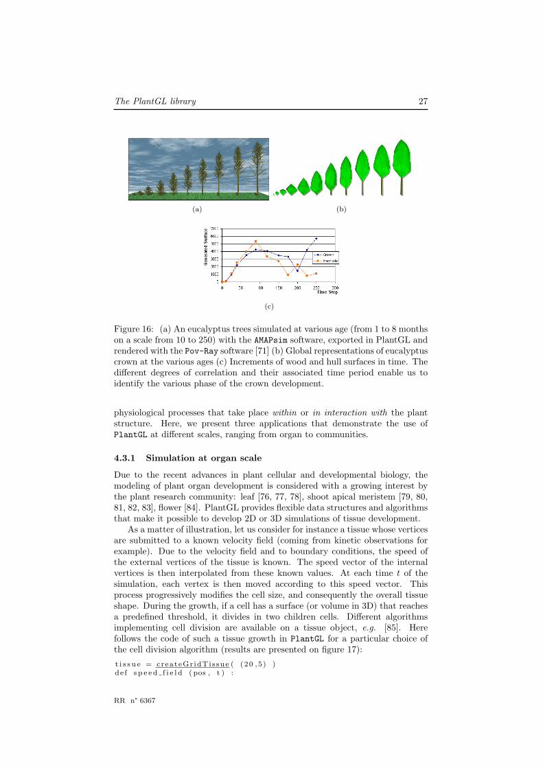
Parametric envelopes provided in PlantGL can also be used to analyse volumet-ric properties of plant crowns. For example, in order to quantify the develop-ment of a plant crown over time, envelopes can be adjusted to the crown ofthe developing tree at different ages and their surface or volume can then beestimated.

Figure 16 illustrates this approach together with the possibility to importplant data from other softwares. The growth of an eucalyptus was simulated atvarious ages using the AMAPsim software [22], Figure 16.a. Results were importedin PlantGL as MTGs. The convex hull of the plant crown was then computedat each age using the fitting algorithms provided by PlantGL for envelopes asdescribed in [14]. Here is how this series of steps can be carried out in PlantGL:import pylabde f h u l l a n a l y s i s ( ages , t r e e s ) :

h u l l s =[ f i t ( ’ convexhul l ’ , i ) f o r i in t r e e s ]wood sf=[ s u r f a c e ( i ) f o r i in t r e e s ]h u l l s f =[ s u r f a c e ( i ) f o r i in hu l l s ]d e l t a wood s f =[wood sf [ i +1]−wood sf [ i ] f o r i in range ( l en ( wood sf )−1)]d e l t a h u l l s f =[ h u l l s f [ i +1]− h u l l s f [ i ] f o r i in range ( l en ( h u l l s f )−1)]pylab . p l o t ( ages [ 1 : ] , d e l t a wood s f )pylab . p l o t ( ages [ 1 : ] , d e l t a h u l l s f )

Based on such data, various investigations about the crown development canbe made. Curves showing the variation of crown surface/volume throughouttime can be analysed, comparison at a more microscopic scale with the leaf areavariation can be made 16.c, etc.

4.3 Simulations based on plant geometric models

Using flexible geometric models of plant is not restricted to the analysis of plantstructure. They can be used as well for the simulation of various physical or

INRIA


(a) (b)

(c)

Figure 16: (a) An eucalyptus trees simulated at various age (from 1 to 8 monthson a scale from 10 to 250) with the AMAPsim software, exported in PlantGL andrendered with the Pov-Ray software [71] (b) Global representations of eucalyptuscrown at the various ages (c) Increments of wood and hull surfaces in time. Thedifferent degrees of correlation and their associated time period enable us toidentify the various phase of the crown development.

physiological processes that take place within or in interaction with the plantstructure. Here, we present three applications that demonstrate the use ofPlantGL at different scales, ranging from organ to communities.

4.3.1 Simulation at organ scale

Due to the recent advances in plant cellular and developmental biology, themodeling of plant organ development is considered with a growing interest bythe plant research community: leaf [76, 77, 78], shoot apical meristem [79, 80,81, 82, 83], flower [84]. PlantGL provides flexible data structures and algorithmsthat make it possible to develop 2D or 3D simulations of tissue development.

As a matter of illustration, let us consider for instance a tissue whose verticesare submitted to a known velocity field (coming from kinetic observations forexample). Due to the velocity field and to boundary conditions, the speed ofthe external vertices of the tissue is known. The speed vector of the internalvertices is then interpolated from these known values. At each time t of thesimulation, each vertex is then moved according to this speed vector. Thisprocess progressively modifies the cell size, and consequently the overall tissueshape. During the growth, if a cell has a surface (or volume in 3D) that reachesa predefined threshold, it divides in two children cells. Different algorithmsimplementing cell division are available on a tissue object, e.g. [85]. Herefollows the code of such a tissue growth in PlantGL for a particular choice ofthe cell division algorithm (results are presented on figure 17):

t i s s u e = crea teGr idTi s sue ( (20 ,5 ) )de f s p e e d f i e l d ( pos , t ) :

RR n° 6367


yspeed=a∗[1+b∗ t ∗pos . xˆ2/(h+b∗ t ) ˆ2 ]∗ exp(−pos . xˆ2/(h+b∗ t ) )r e turn Vector (0 , yspeed )

f o r t in range ( t ime begin , time end , d e l t a t ime ) :f o r pos in t i s s u e . p o s i t i o n s ( ) :

pos+=s p e e d f i e l d ( pos , t )∗ de l t a t imef o r c e l l in t i s s u e :

i f c e l l . s i z e ( ) > max c e l l s i z e :c e l lD i v i d e ( c e l l , a lgo=MAIN AXIS)

(a) (b) (c)

(d)

Figure 17: (a,b,c) 2D geometrical representation of a growing tissue at threedifferent times. (d) 3D simulation of bump formation on a tissue

4.3.2 Simulation at plant scale

In biological applications, virtual plants are frequently used to carry out virtualexperiments where data is difficult to measure or when the interaction betweenthe studied processes is too complex. This is particularly true for the study oflight interception by plants: light cannot be measured in a real canopy withhigh accuracy and the amount of light rays that can go through a canopy is acomplex function of the tree architecture. The following example illustrates theuse of PlantGL in the context of model assessment and how high-level geomet-ric operations used in light interception models can be simply performed withPlantGL.

The STAR (Surface to Total Area Ratio) is a key eco-physiological parameterused in light interception models [86]. It is a directional quantity defined byratioing the surface of the projection of a tree foliage SΩ in a particular directionΩ to its total leaf surface S.

STARΩ =SΩ

S(12)

This directional index can be integrated over all the sky vault to characterizethe overall light interception of a tree.

INRIA


However, since the total leaf area of a real plant is often expensive to measure,approximate values of the STAR are often used in place of the exact one ineco-physiological applications. For this, the directional STAR is estimated fromsimple measures of the plant volume and leaf density and by making simplifyingassumptions on the actual spatial distribution of leaves in the canopy [87]. Inthis case, the plant is supposed to be an homogeneous volume with small leavesuniformly distributed within the crown looking like a “turbid medium”. In thiscontext, a light beam b of direction Ωb has a probability p0(b) to be intercepted:

p0(b) = exp (−GΩb.LAD.lb) (13)

where GΩbis a coefficient characterizing the spatial distribution of leaf ori-

entations in the crown volume, LAD is the Leaf Area Density in the volume andlb the length of the beam path in the crown volume. Assuming the B beamsconstitute a regular and dense sampling of the whole volume, the approximateddirectional STAR of the turbid volume, STARΩ, can then be computed as [88]:

STARΩ =B∑

b=1

Sb(1− p0(b))/S (14)

where Sb is the cross section area of a beam. This model-based definitionof the STAR can be compared to the above real STAR to evaluate the qualityof light model assumptions. The resulting difference characterizes the error dueto the model underlying hypotheses (homogeneity/randomness of the foliagedistribution, negligibility of leaf size, ...) with respect to the actual canopies[87].

In PlantGL, both STAR quantities, i.e. the real and approximated STARs,can be computed from a plant mockup using the library high-level functions.The real STAR of a given virtual canopy can be computed by counting thenumber of vegetation pixels in a virtual picture obtained by projecting virtualplant canopies using an orthographic camera [87] and multiplying by the size ofa pixel. This would be expressed as follows in PlantGL:

de f s t a r ( l eaves , d i r ) :Viewer . d i sp l ay ( l e av e s )Viewer . camera . se tOrthographic ( )Viewer . camera . s e tD i r e c t i o n ( d i r )proj , nbpixe l , p i x e l s i z e = Viewer . frameGL . g e tP r o j e c t i o nS i z e ( )re turn pro j / su r f a c e ( l e av e s )

For the approximated STAR, the envelope of the tree crown must first becomputed. Then, a set of beams of direction Ω are cast and their interceptionsand resulting length in the crown volume are computed. A sketch of such a codewould be as follows:

de f s t a r ( l eaves , g , d i r , up , r i ght , beam radius ) :hu l l= f i t ( ’ convexhul l ’ , l e a v e s )lad = su r f a c e ( l e av e s ) / volume ( hu l l )bbx = BoundingBox ( hu l l , d i r , up , r i g h t )Viewer . d i sp l ay ( hu l l )pos = bbx . upperRightCorner ( )i n t e r c e p t i o n = 0f o r r s h i f t in range (bbx . s i z e ( ) . y/ beam radius ) :

f o r up sh i f t in range (bbx . s i z e ( ) . z/ beam radius ) :

RR n° 6367


ray = Viewer . castRay ( pos−r s h i f t ∗ r i ght−up sh i f t ∗up , d i r )p0 = 1f o r i n t e r s e c t i o n in ray :

l ength = norm( i n t e r s e c t i o n [1]− i n t e r s e c t i o n [ 0 ] )p0 ∗= exp(−g∗ l ad ∗ l ength )

i n t e r c e p t i o n += (1−p0 )∗ ( beam radius ∗∗2)re turn i n t e r c e p t i o n / su r f a c e ( l e av e s )

(a) (b) (c)

Figure 18: Light intercepted by an apple tree represented as shadow on theground. Intensity of the colors represent intensity of interception. STAR canbe computed as a ratio between the surface of the shadow and the plant leafsurface (a) Light intercepted from top direction using ray casting (b) Lightintercepted from same direction using Beer-Lambert hypothesis. (c) Light in-terception sampled from different directions. The different colors are used tomark the difference between various elevations of ray direction.

4.3.3 Simulation at community scale

Detailed plant models, at the level of branches and leaves, do not always cor-respond to the most adequate level for expressing knowledge in plant models.PlantGL provides a number of means to deal with abstract representation ofplants at different scales. In particular, the various envelope models defined insection 3.2.1 can be used as abstract means to model plant crown bulk. Suchmodels are useful for instance in the modeling of plant communities, wherecompetition for space has been shown to be a key structuring factor [89].

In the following example, we illustrate how natural scenes containing thou-sands of plants distributed in a realistic manner can be built with PlantGL,taking into account competition for space. It is inspired by [30] which is anextension of [90, 91] to the use of more complex crown shapes.

The ecosystem synthesis starts with the generation of a set of coarse individ-uals with height, crown radius and crown base height determined from densityand allometric functions.

Individuals are fagus beech trees with different classes of ages. Allometricfunctions of the Fagacees model [92] are used to determine the heights andradius values as a function of tree age. The spatial distribution of these plantsis generated using a stochastic point process. For this, we use a Gibbs process

INRIA


[93, 94] defined as a pairwise interaction function f(pi, pj), that represents thecost associated with the presence of two given plants at positions pi and pj

respectively. Positive cost values will lead to repulsion between trees whilenegative ones lead to attraction. A realization of this process is intended tominimize of the global cost F =

∑i 6=j f(pi, pj), defined as the sum of the costs

associated with each pair of points. The Gibbs process is simulated with aclassical depletion-replacement iterative algorithm [95].

Classically, the cost function is used to model neighbor competition and isdefined as a function of the crown radii and positions of the trees. The costfunction of two trees i and j, characterized by shapes with constant radius, maybe chosen for instance proportional to the difference between the sum of thecrown radii and the distance between pi and pj . For asymmetric shapes, thesame function can be used where radii of trees now correspond to the radius ofeach envelope in the direction defined by the tree positions pi and pj . In addi-tion, both the position and the different parameters of the crown envelope cannow be changed in the depletion-replacement algorithm. Figure 19 illustratesthe 3D output of such a process.

Figure 19: A front and top view of a generated stand at the crown scale.Different colors are used to differentiate various layers of vegetation.

From this set of coarse individuals, detailed plant representations can beinferred and assembled into a complete scene. For this, different generationmethods either available in PlantGL or outside of the software can be used. Inour example, we generated the beech trees using the L-systems models usinggenerative procedure described in [29].

Bushes and flowers were generated using PlantGL and Python as presentedin section 3.3 and added to the scene. Finally, a digitized walnut tree [68] wasalso added to illustrate how scenes may be created in PlantGL using a range ofclassical date sources.

The final rendering was made with Povray [71]. Each plant geometric modelswere thus converted and assembled in this format. Figure 20 illustrates theresulting scene.

5 Conclusion

In this paper, we presented a new open-software library for the geometric mod-eling of plants built on the top of the Python programming language. The

RR n° 6367


Figure 20: A community of plants generated from a Gibbs process [30]. Thescene is made of trees coming from different sources: beech trees of different sizesand ages where generated using the ecosystem model presented in section 4.3.3which were built using the interaction between PlantGL and LStudio/Vlab, Awalnut tree corresponding to a 3D digitizing of a real plant built using AMAP-mod/VPlants, virtual bushes flowers and grass created procedurally in Pythonwith PlantGL

library provides a set of geometric models that are useful to represent vari-ous types of plant structures at different scales, ranging from tissues to plantcommunities. In particular, it contains original geometric components such asdedicated parametric envelopes for crown shape representation and tissues forrepresenting plants at cell scale in 2D or 3D. Branching systems can be cre-ated either procedurally or by importing them from plant growth simulationplatforms, such as LStudio/VLab. The resulting plant geometric models can beeasily analysed using Python and PlantGL high level algorithms. The differentfeatures of the PlantGL library have been illustrated on applications involvingplants at different scales and showing its use at various stages of a modelingprocess.

Acknowledgments.

The authors thank P. Prusinkiewicz for making the LStudio/VLab softwarekindly available to them, D. Da Silva, P. Barbier de Reuille and Y. Caragliofor their contribution to some images, and H. Sinoquet, E. Costes, F. Danjon,C.-E. Parveau and J. Traas for making 3D digitized plants or tissues availableto them. This work has been partially supported by ANR projects NatSim andVirtual Carpel.

INRIA


References

[1] P. Prusinkiewicz, A. Lindenmayer, The algorithmic beauty of plants,Springer-Verlag New York, Inc., New York, NY, USA, 1990.

[2] P. de Reffye, C. Edelin, J. Francon, M. Jaeger, C. Puech, Plant mod-els faithful to botanical structure and developmentr, in: SIGGRAPH ’88:Proceedings of the 15th annual conference on Computer graphics and in-teractive techniques, New York, NY, USA, 1988, pp. 151–158.

[3] J. Weber, J. Penn, Creation and rendering of realistic trees, in: SIGGRAPH’95: Proceedings of the 22nd annual conference on Computer graphics andinteractive techniques, ACM Press, New York, NY, USA, 1995, pp. 119–128.

[4] B. Lintermann, O. Deussen, Interactive modeling of plants, ComputerGraphics and Applications, IEEE 19 (1) (1999) 56–65.

[5] P. Prusinkiewicz, L. Mundermann, R. Karwowski, B. Lane, The use of posi-tional information in the modeling of plants, in: SIGGRAPH’01, ComputerGraphics, ACM, Los Angeles, California, 2001, pp. 36–47.

[6] I. Shlyakhter, M. Rozenoer, J. Dorsey, S. Teller, Reconstructing 3d treemodels from instrumented photographs, IEEE Comput. Graph. Appl.21 (3) (2001) 53–61.

[7] N. B., T. Franken, O. Deussen, Approximate image-based tree-modelingusing particle flows, ACM Transactions on Graphics (Proc. of SIGGRAPH2007) 26 (3).

[8] P. Tan, G. Zeng, J. Wang, S.-B. Kang, L. Quan, Image-based tree modeling,ACM Transactions on Graphics (Proc. of SIGGRAPH 2007) 26 (3).

[9] A. Cescatti, Modelling the radiative transfer in discontinuous canopies ofasymmetric crown. I. model structure and algorithms, Ecological Modelling101 (1997) 263–274.

[10] H. Sinoquet, P. Rivet, C. Godin, Assessment of the three-dimensional archi-tecture of walnut trees using digitising, Silva Fennica 31 (3) (1997) 265–273.

[11] C. Godin, Representing and encoding plant architecture: a review, Annalsof Forest Science 57 (05-juin) (2000) 413–438.

[12] F. Danjon, H. Sinoquet, C. Godin, F. Colin, M. Drexhage, Characterisa-tion of structural tree root architecture using 3d digitising and amapmodsoftware, Plant and Soil 211 (2) (1999) 241–258.

[13] J. B. Evers, J. Vos, C. Fournier, B. Andrieu, M. Chelle, P. C. Struik, To-wards a generic architectural model of tillering in gramineae, as exemplifiedby spring wheat (triticum aestivum)., New Phytol 166 (3) (2005) 801–812.

[14] F. Boudon, C. Godin, C. Pradal, O. Puech, H. Sinoquet, Estimating thefractal dimension of plants using the two-surface method. an analysis basedon 3d-digitized tree foliage, Fractals 14 (3) (2006) 149–163.

RR n° 6367


[15] R.-S. Smith, C. Kuhlemeier, P. Prusinkiewicz, Inhibition fields for phyl-lotactic pattern formation: a simulation study, Canadian Journal of Botany84 (2006) 1635–1649.

[16] A. Lindenmayer, Mathematical models for cellular interactions in develop-ment, I & II, Journal of Theoretical Biology (1968) 280–315.

[17] R. Karwowski, P. Prusinkiewicz, Design and implementation of the l+cmodeling language, Electronic Notes in Theoretical Computer Science 86.

[18] P. Prusinkiewicz, R. Karwowski, B. Lane, The l+c plant modeling lan-guage, in: J. V. et al. (Ed.), Functional-Structural Plant Modelling in CropProduction, Springer, 2007, p. in press.

[19] W. Kurth, Growth grammar interpreter grogra 2.4: A software forthe 3-dimentional interpretation of stochastic, sensitive growth grammarin the context of plant modelling, Introduction and reference manual,Forschungszentrum Waldokosysteme der Universitat Gottingen (1994).

[20] O. Kniemeyer, G.-H. Buck-Sorlin, K. W., A graph grammar approach toartificial life, Artificial Life 10 (4) (2004) 413–431.

[21] G.-H. Buck-Sorlin, O. Kniemeyer, W. Kurth, Barley morphology, geneticsand hormonal regulation of internode elongation modelled by a relationalgrowth grammar, New Phytologist 10 (4) (2005) 413–431.

[22] J.-F. Barczi, P. de Reffye, Y. Caraglio, Essai sur l’identifcation et la miseen oeuvre des parametres necessaires a la simulation d’une architecturevegetale : le logiciel amapsim., in: J. Bouchon, P. de Reffye, D. Barthelemy(Eds.), Modelisation et Simulation de l’Architecture des Vegetaux, INRAEditions, 1997, pp. 205 – 254.

[23] O. Deussen, B. Lintermann, Digital Design of Nature. Computer GeneratedPlants and Organics., Springer-Verlag, 2005.

[24] C. Godin, E. Costes, Y. Caraglio, Exploring plant topological structurewith the amapmod software: an outline, Silva Fennica 31 (1997) 355–366.

[25] C. Godin, E. Costes, H. Sinoquet, A method for describing plant architec-ture which integrates topology and geometry, Annals of Botany 84 (1999)343–357.

[26] E. Costes, H. Sinoquet, J.-J. Kelner, C. Godin, Exploring within-tree ar-chitectural development of two apple tree cultivars over 6 years, Annals ofBotany 91 (2003) 91–104.

[27] P. Ferraro, C. Godin, P. Prusinkiewicz, Toward a quantification of self-similarity in plants, Fractals 13 (2) (2005) 91–109.

[28] Y. Guedon, Y. Caraglio, P. Heuret, E. Lebarbier, C. Meredieu, Analyzinggrowth components in trees, Journal of Theoretical Biology.

[29] F. Boudon, P. Prusinkiewicz, C. Federl, P.and Godin, R. Karwowski, In-teractive design of bonsai tree models, Computer Graphics Forum (Proc.of Eurographics ’03) 22 (3) (2003) 591–591.

INRIA


[30] F. Boudon, G. Le Moguedec, Deformation asymetrique de houppiers pourla generation de representations paysageres realistes, Revue ElectroniqueFrancophone d’Informatique Graphique (REFIG) 1 (1).

[31] F. Danjon, T. Fourcaud, D. Bert, Root architecture and wind-firmness ofmature pinus pinaster., New Phytol 168 (2) (2005) 387–400.

[32] P. Barbier de Reuille, I. Bohn-Courseau, C. Godin, J. Traas, A protocol toanalyse cellular dynamics during plant development, The Plant Journal 44(2005) 1045–1053.

[33] D. Da Silva, F. Boudon, C. Godin, O. Puech, C. Smith, H. Sinoquet, Acritical appraisal of the box counting method to assess the fractal dimensionof tree crowns., Lecture Notes in Computer Sciences (Proceedings of the2nd International Symposium on Visual Computing).

[34] G. Louarn, Y. Guedon, J. Lecoeur, E. Lebon, Quantitative analysis of thephenotypic variability of shoot architecture in two grapevine cultivars (vitisvinifera l.)., Annals of Botany 99 (3) (2007) 425–437.

[35] J. Chopard, C. Godin, J. Traas, Toward a formal expression of morpho-genesis: a mechanics based integration of cell growth at tissue scale, in:Proceedings of the 7th International Workshop on Information Processingin Cell And Tissues, Oxford, UK, 2007, p. in press.

[36] E. Gamma, R. Helm, R. Johnson, J. Vlissides, Design Patterns: Elementsof Reusable Object-Oriented Software, Addison-Wesley, 1995.

[37] P. S. Strauss, R. Carey, An object-oriented 3d graphics toolkit, in: SIG-GRAPH ’92: Proceedings of the 19th annual conference on Computergraphics and interactive techniques, ACM Press, New York, NY, USA,1992, pp. 341–349.

[38] C. B. Barber, D. P. Dobkin, H. Huhdanpaa, The quickhull algorithm forconvex hulls, ACM Trans. Math. Softw. 22 (4) (1996) 469–483.

[39] E. Welzl, Smallest enclosing disks (balls and ellipses), New Results andNew Trends in Computer Science 555 (1991) 359–370.

[40] E. Andres, P. Nehlig, J. Francon, Supercover of straight lines, planes andtriangles, in: DGCI ’97: Proceedings of the 7th International Workshop onDiscrete Geometry for Computer Imagery, Springer-Verlag, London, UK,1997, pp. 243–254.

[41] R. Carey, G. Bell, The Annotated VRML 2.0 Reference Manual, Addison-Wesley, 2002.

[42] F. Boudon, C. Nouguier, C. Godin, Geom module manual. I. user’s guide,Document de travail du Programme Modelisation des plantes 3-2001,CIRAD (12/2001 2001).

[43] J.-G. Schneider, O. Nierstrasz, Components, scripts and glue., in: L. Bar-roca, J. Hall, P. Hall (Eds.), Software Architectures - Advances and Appli-cations, Springer, 1999, Ch. 2, pp. 13–25.

RR n° 6367


[44] T. E. Oliphant, Python for scientific computing, Computing in Science andEngineering 9 (3) (2007) 10–20.

[45] H. Sowizral, Scene graphs in the new millennium, IEEE Comput. Graph.Appl. 20 (1) (2000) 56–57.

[46] S. Meyers, More Effective C++: 35 New Ways to Improve Your Programsand Designs, Addison-Wesley Longman Publishing Co., Inc., Boston, MA,USA, 1995.

[47] Boost c++ librairies (1998–2006).URL http://www.boost.org/

[48] J. Phattaralerphong, H. Sinoquet, A method for 3d reconstruction of treecrown volume from photographs: assessment with 3d-digitized plants, TreePhysiology 25.

[49] A. Reche-Martinez, I. Martin, G. Drettakis, Volumetric reconstruction andinteractive rendering of trees from photographs, ACM Trans. Graph. 23 (3)(2004) 720–727.

[50] H. Horn, The adaptive geometry of trees, Princeton University Press,Princeton, N.J., 1971.

[51] H. Koop, Silvi-star: A comprehensive monitoring system, Forest Dynamics(1989) 229.

[52] P. Birnbaum, Modalites d’occupation de l’espace par les arbres en foretsguyanaise, Master’s thesis, Universite Paris VI (1997).

[53] C. D. Woodward, Skinning techniques for interactive b-spline surface in-terpolation, Comput. Aided Des. 20 (10) (1988) 441–451.

[54] L. A. Piegl, W. Tiller, The Nurbs Book, 2nd Edition, Springer, 1997.

[55] L. A. Piegl, W. Tiller, Surface skinning revisited, The Visual Computer18 (4) (2002) 273–283.

[56] M. Barnsley, Fractals Everywhere, Academic Press, Boston, 1988.

[57] K. Falconer, Techniques in fractal geometry, John Wiley and Sons, 1997.

[58] C. Godin, Y. Caraglio, A multiscale model of plant topological structures,Journal of theoretical biology 191 (1998) 1–46.

[59] R. Mech, M. James, M. Hammel, J. Hanan, P. Prusinkiewicz, CPFG v4.0user manual, The University of Calgary (2005).

[60] C. Godin, E. Costes, H. Sinoquet, A method for describing plant architec-ture which integrates topology and geometry, Annals of Botany 84 (1999)343–357.

[61] F. Boudon, Representation geometrique multi-echelles de l’architecture desplantes, Ph.D. thesis, Universite de Montpellier II (2004).

INRIA

http://www.boost.org/


[62] P. Prusinkiewicz, Graphical applications of l-systems, in: Proceedings onGraphics Interface ’86/Vision Interface ’86, Canadian Information Process-ing Society, Toronto, Ont., Canada, Canada, 1986, pp. 247–253.

[63] C. Godin, Y. Guedon, E. Costes, Exploration of a plant architecturedatabase with the amamod software illustrated on an apple tree hybridfamily, Agronomie 19 (3-4).

[64] B. Adam, N. Dones, H. Sinoquet, Vegestar v.3.1. a software to computelight interception and photosynthesis by 3d plant mock-ups, in: C. Godin(Ed.), Fourth International Workshop on Functional-Structural Plant Mod-els, Montpellier, France, 2004, p. 414.

[65] E. H. Spanier, Algebraic Topology, McGraw-Hill, New York, 1966.

[66] Cgal, Computational Geometry Algorithms Library.URL http://www.cgal.org

[67] H. Sinoquet, B. Andrieu, The geometrical structure of plant canopies: char-acterization and direct measurements methods, in: C. Varlet-Grancher,R. Bonhomme, H. Sinoquet (Eds.), Crop structure and light microclimate,Vol. 0, INRA Editions, Paris, 1993, pp. 131–158.

[68] H. Sinoquet, P. Rivet, C. Godin, Assessment of the three-dimensional ar-chitecture of walnut trees using digitizing, Silva Fennica 3 (1997) 265–273.

[69] C.-E. Parveaud, Proprietes radiatives des couronnes de noyers (Juglans ni-gra x J. regia) et croissance des pousses annuelles - influence de la geometriedu feuillage, de la position des pousses et de leur climat radiatif, Ph.D. the-sis, Universite de Montpellier II, France (2006).

[70] E. Casella, H. Sinoquet, A method for describing the canopy architectureof coppice poplarwith allometric relationships., Tree Physiology 23 (2003)1153–1170.

[71] T. P.-R. Team, Persistence of vision raytracer (1991–2006).URL http://www.povray.org/

[72] B. B. Mandelbrot, The fractal geometry of nature, W.N. Freeman, NewYork, USA, 1983.

[73] E. Costes, H. Sinoquet, C. Godin, J. J. Kelner, 3d digitizing based on treetopology : application to study the variability of apple quality within thecanopy, Acta Horticulturae 499 (1999) 271–280.

[74] M. Barnsley, S. Demko, Iterated Function Systems and the Global Con-struction of Fractals, Royal Society of London Proceedings Series A 399(1985) 243–275.

[75] A. L. Oppelt, W. Kurth, H. Dzierzon, G. Jentschke, D. L. Godbold, Struc-ture and fractal dimensions of root systems of four co-occurring fruit treespecies from Botswana, Annals of Forest Science 57 (2000) 463–475.

RR n° 6367

http://www.cgal.org

http://www.povray.org/


[76] J. Runions, T. Brach, S. Kuhner, Photoactivation of gfp reveals proteindynamics within the endoplasmic reticulum membrane, Journal of Experi-mental Botany 57 (1) (2006) 43–50.

[77] F. G. Feugier, Models of vascular pattern formation in leaves, Ph.D. thesis,Pierre et Marie Curie (2005).

[78] A.-G. Rolland-Lagan, E. Coen, S. J. Impey, J. A. Bangham, A computa-tional method for inferring growth parameters and shape changes duringdevelopment base clonal analysis, Journal of Theoretical Biology 232 (2005)157–177.

[79] H. Jonsson, M. Heisler, G. V. Reddy, V. Agrawal, V. Gor, B. E. Shapiro,E. Mjolsness, E. M. Meyerowitz, Modeling the organization of the wuschelexpression domain in the shoot apical meristem., Bioinformatics 21 Suppl1.

[80] H. Jonsson, M. G. Hesler, B. E. Shapiro, E. M. Meyerowitz, E. Mjolsness,An auxin-driven polarized transport model for phyllotaxis, PNAS 103 (5)(2006) 1633–1638.

[81] P. Barbier de Reuille, I. Bohn-Courseau, K. Ljung, H. Morin, N. Carraro,C. Godin, J. Traas, Computer simulations reveal properties of the cell-cellsignaling network at the shoot apex in arabidopsis, PNAS 103 (5) (2006)1627–1632.

[82] C. Smith, On vertex-vertex systems and their use in geometric and biolog-ical modelling, Ph.D. thesis, University of Calgary (2006).

[83] M. Heisler, H. Jonsson, Modelling meristem development in plants, CurrentOpinion in Plant Biology 10 (2007) 92–97.

[84] A.-G. Rolland-Lagan, J. A. Bangham, E. Coen, Growth dynamics under-lying petal shape and asymmetry, Nature 422 (13) (2003) 161–163.

[85] J. Nakielski, Tensorial model for growth and cell division in the shoot apex,in: A. Carbone, M. Gromov, P. Prusinkiewicz (Eds.), Pattern formation inbiology, vision and dynamics, World Scientific, Singapore, 2000, pp. 252–267.

[86] P. Oker-Blom, H. Smolander, The ratio of shoot silhouette area to totalneedle area in scots pine, Forest Science 34 (1988) 894–906.

[87] H. Sinoquet, G. Sonohat, J. Phattaralerphong, C. Godin, Foliage random-ness and light interception in 3-d digitized trees: an analysis from mul-tiscale discretization of the canopy, Plant, Cell and Environment 28 (9)(2005) 1158–1170.

[88] H. Sinoquet, C. Varlet-Granchet, R. Bonhomme, Modelling radiative trans-fer within homogeneous canopies: basic concepts, in: C. Varlet-Grancher,R. Bonhomme, H. Sinoquet (Eds.), Crop structure and light microclimate,Vol. 0, INRA Editions, Paris, 1993, pp. 131–158.

[89] A. Franc, S. Gourlet-Fleury, N. Picard, Une introduction a la modelisationdes forets heterogenes, ENGREF, Nancy, 2000.

INRIA


[90] O. Deussen, P. Hanrahan, B. Lintermann, R. Mech, M. Pharr,P. Prusinkiewicz, Realistic modeling and rendering of plant ecosystems,Computer Graphics 32 (Annual Conference Series) (1998) 275–286.

[91] B. Lane, P. Prusinkiewicz, Generating spatial distributions for multilevelmodels of plant communities, in: Proceedings of Graphics Interface 2002,Calgary, Alberta, 2002, pp. 69–80.

[92] G. Le Moguedec, J. Dhote, Presentation du modele Fagacees, Tech. rep.,LERFOB, INRA, Nancy, France (2002).

[93] P. Diggle, Statistical analysis of spatial point patterns, Academic Press,London, UK, 1983.

[94] F. Goreaud, Apport de l’analyse de la structure spatiale en foret tempereea l’etude de la modelisation des peuplements complexes, Ph.D. thesis, EN-GREF (2004).

[95] B. Rippley, Simulating spatial patterns: dependent samples from a multi-variate density, Applied Statistic 28 (1979) 109–112.

RR n° 6367

Centre de recherche INRIA Sophia Antipolis – Méditerranée2004, route des Lucioles - BP 93 - 06902 Sophia Antipolis Cedex (France)

Centre de recherche INRIA Futurs : Parc Club Orsay Université - ZAC des Vignes4, rue Jacques Monod - 91893 ORSAY Cedex (France)

Centre de recherche INRIA Nancy – Grand Est : LORIA, Technopôle de Nancy-Brabois - Campus scientifique615, rue du Jardin Botanique - BP 101 - 54602 Villers-lès-Nancy Cedex (France)

Centre de recherche INRIA Rennes – Bretagne Atlantique : IRISA, Campus universitaire de Beaulieu - 35042 Rennes Cedex (France)Centre de recherche INRIA Grenoble – Rhône-Alpes : 655, avenue de l’Europe - 38334 Montbonnot Saint-Ismier (France)

Centre de recherche INRIA Paris – Rocquencourt : Domaine de Voluceau - Rocquencourt - BP 105 - 78153 Le Chesnay Cedex (France)

ÉditeurINRIA - Domaine de Voluceau - Rocquencourt, BP 105 - 78153 Le Chesnay Cedex (France)

http://www.inria.frISSN 0249-6399

plantgl: a python-based geometric library for 3d plant modelling at

Documents