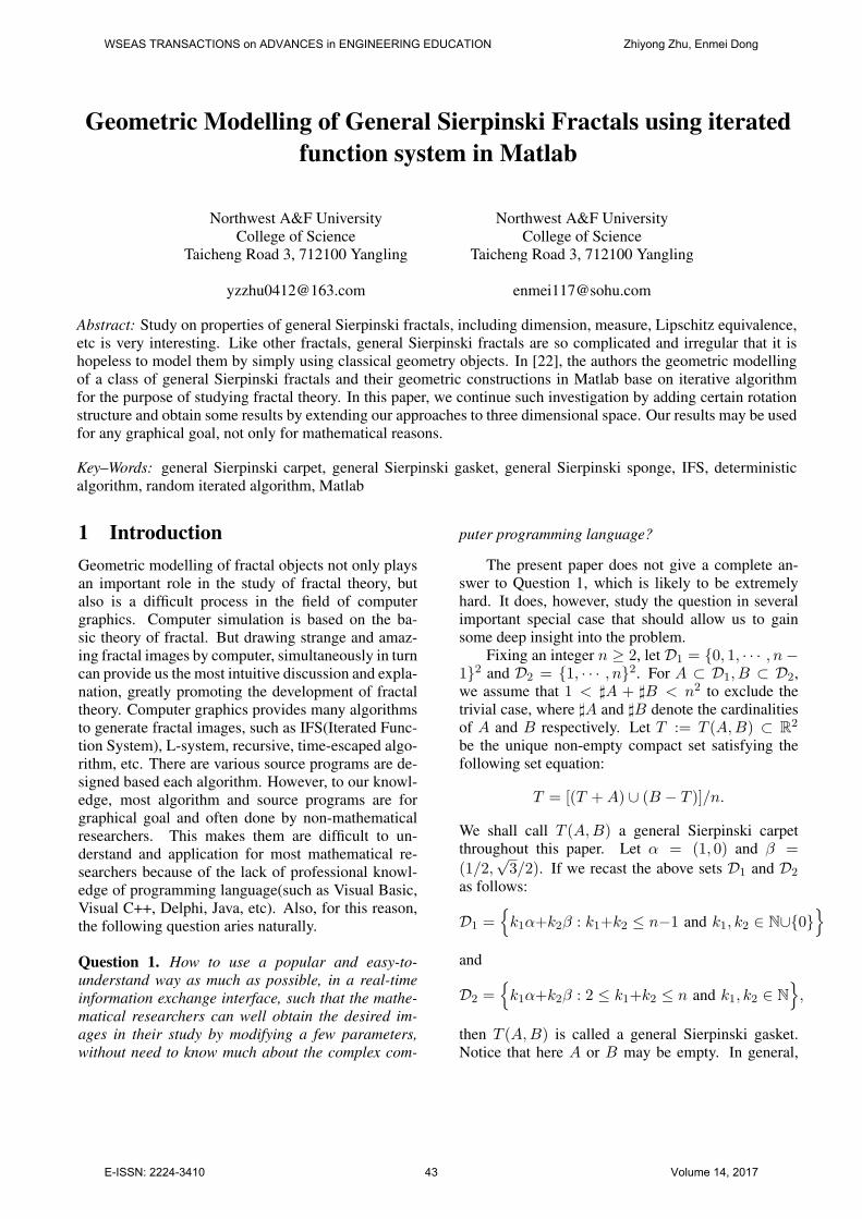
geometric modelling of general sierpinski fractals using ... · geometric modelling of general...
TRANSCRIPT
Geometric Modelling of General Sierpinski Fractals using iteratedfunction system in Matlab
Zhiyong ZhuNorthwest A&F University
College of ScienceTaicheng Road 3, 712100 Yangling
Enmei Dong*Northwest A&F University
College of ScienceTaicheng Road 3, 712100 Yangling
Abstract: Study on properties of general Sierpinski fractals, including dimension, measure, Lipschitz equivalence,etc is very interesting. Like other fractals, general Sierpinski fractals are so complicated and irregular that it ishopeless to model them by simply using classical geometry objects. In [22], the authors the geometric modellingof a class of general Sierpinski fractals and their geometric constructions in Matlab base on iterative algorithmfor the purpose of studying fractal theory. In this paper, we continue such investigation by adding certain rotationstructure and obtain some results by extending our approaches to three dimensional space. Our results may be usedfor any graphical goal, not only for mathematical reasons.
Key–Words: general Sierpinski carpet, general Sierpinski gasket, general Sierpinski sponge, IFS, deterministicalgorithm, random iterated algorithm, Matlab
1 IntroductionGeometric modelling of fractal objects not only playsan important role in the study of fractal theory, butalso is a difficult process in the field of computergraphics. Computer simulation is based on the ba-sic theory of fractal. But drawing strange and amaz-ing fractal images by computer, simultaneously in turncan provide us the most intuitive discussion and expla-nation, greatly promoting the development of fractaltheory. Computer graphics provides many algorithmsto generate fractal images, such as IFS(Iterated Func-tion System), L-system, recursive, time-escaped algo-rithm, etc. There are various source programs are de-signed based each algorithm. However, to our knowl-edge, most algorithm and source programs are forgraphical goal and often done by non-mathematicalresearchers. This makes them are difficult to un-derstand and application for most mathematical re-searchers because of the lack of professional knowl-edge of programming language(such as Visual Basic,Visual C++, Delphi, Java, etc). Also, for this reason,the following question aries naturally.
Question 1. How to use a popular and easy-to-understand way as much as possible, in a real-timeinformation exchange interface, such that the mathe-matical researchers can well obtain the desired im-ages in their study by modifying a few parameters,without need to know much about the complex com-
puter programming language?
The present paper does not give a complete an-swer to Question 1, which is likely to be extremelyhard. It does, however, study the question in severalimportant special case that should allow us to gainsome deep insight into the problem.
Fixing an integer n ≥ 2, let D1 = {0, 1, · · · , n−1}2 and D2 = {1, · · · , n}2. For A ⊂ D1, B ⊂ D2,we assume that 1 < ]A + ]B < n2 to exclude thetrivial case, where ]A and ]B denote the cardinalitiesof A and B respectively. Let T := T (A,B) ⊂ R2
be the unique non-empty compact set satisfying thefollowing set equation:
T = [(T + A) ∪ (B − T )]/n.
We shall call T (A,B) a general Sierpinski carpetthroughout this paper. Let α = (1, 0) and β =(1/2,
√3/2). If we recast the above sets D1 and D2
as follows:
D1 ={
k1α+k2β : k1+k2 ≤ n−1 and k1, k2 ∈ N∪{0}}
and
D2 ={
k1α+k2β : 2 ≤ k1+k2 ≤ n and k1, k2 ∈ N}
,
then T (A,B) is called a general Sierpinski gasket.Notice that here A or B may be empty. In general,
WSEAS TRANSACTIONS on ADVANCES in ENGINEERING EDUCATION Zhiyong Zhu, Enmei Dong
E-ISSN: 2224-3410 43 Volume 14, 2017
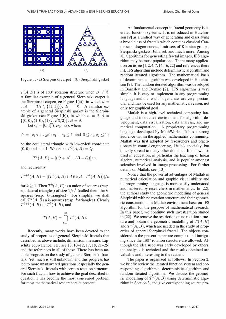
(a) (b)
Figure 1: (a) Sierpinski carpet (b) Sierpinski gasket
T (A,B) is of 180◦ rotation structure when B 6= ∅.A familiar example of a general Sierpinski carpet isthe Sierpinski carpet(see Figure 1(a)), in which n =3, A = D1 \ {(1, 1)}}, B = ∅. A familiar ex-ample of a general Sierpinski gasket is the Sierpin-ski gasket (see Figure 1(b)), in which n = 2, A ={(0, 0), (1, 0), (1/2,
√3/2)}, B = ∅.
Let Q = [0, 1]2(resp. 4), where
4 = {c1α + c2β : c1 + c2 ≤ 1 and 0 ≤ c1, c2 ≤ 1}
be the equilateral triangle with lower-left coordinate(0, 0) and side 1. We define T 0(A,B) = Q,
T 1(A,B) = [(Q + A) ∪ (B −Q)]/n,
and recurrently,
T k+1(A,B) = [(T k(A,B)+A)∪(B−T k(A,B))]/n
for k ≥ 1. Then T k(A,B) is a union of squares (resp.equilateral triangles) of size 1/nk (called them the k-squares (resp. k-triangles)). For simplify, we shallcall T k(A,B) a k-squares (resp. k-triangles). ClearlyT k+1(A,B) ⊂ T k(A,B), and
T (A,B) =∞⋂
k=1
T k(A,B).
Recently, many works have been devoted to thestudy of properties of general Sierpinski fractals thatdescribed as above include, dimension, measure, Lip-schitz equivalence, etc, see [8, 10–12, 17, 18, 21–25]and the references in all of these. There has been no-table progress on the study of general Sierpinski frac-tals. Yet much is still unknown, and this progress hasled to more unanswered questions, especially the gen-eral Sierpinski fractals with certain rotation structure.For such fractal, how to achieve the goal described inquestion 1 has become the most concerned problemfor most mathematical researchers at present.
An fundamental concept in fractal geometry is it-erated function systems. It is introduced in Hutchin-son [9] as a unified way of generating and classifyinga broad class of fractals which contains classical Can-tor sets, dragon curves, limit sets of Kleinian groups,Sierpinski gaskets, Julia set, and much more. Amongall algorithms for generating fractal images, IFS algo-rithm may be most popular one. There many applica-tion on it(see [1,2,4,7,14,16,22] and references therein). IFS algorithm include deterministic algorithm andrandom iterated algorithm. The mathematical basisof deterministic algorithm was developed in Hutchin-son [9]. The random iterated algorithm was developedin Barnsley and Demko [2]. IFS algorithm is verysimple, it is easy to implement in any programminglanguage and the results it generates are very spectac-ular and may be used for any mathematical reason, notonly for graphical goal.
Matlab is a high-level technical computing lan-guage and interactive environment for algorithm de-velopment, data visualization, data analysis, and nu-merical computation. A proprietary programminglanguage developed by MathWorks. It has a strongaudience within the applied mathematics community.Matlab was first adopted by researchers and practi-tioners in control engineering, Little’s specialty, butquickly spread to many other domains. It is now alsoused in education, in particular the teaching of linearalgebra, numerical analysis, and is popular amongstscientists involved in image processing. For furtherdetails on Matlab, see [13].
Notice that the powerful advantages of Matlab innumerical calculation and graphic visual ability andits programming language is more easily understoodand mastered by researchers in mathematics. In [22],the authors study the geometric modelling of generalSierpinski with no rotation structure and their geomet-ric constructions in Matlab environment base on IFSalgorithm for the purpose of mathematical research.In this paper, we continue such investigation startedin [22]. We remove the restriction on no rotation struc-ture and obtain the geometric modelling of T (A,B)and T k(A,B), which are needed in the study of prop-erties of general Sierpinski fractal. The objects con-sidered in the present paper are complex and intrigu-ing since the 180◦ rotation structure are allowed. Al-though the idea used was early developed by others,the analysis is technical and the results obtained arevaluable and interesting to the readers.
The paper is organized as follows: In Section 2,we briefly review the iterated function system and cor-responding algorithms: deterministic algorithm andrandom iterated algorithm. We discuss the geomet-ric modelling of T k(A,B) using deterministic algo-rithm in Section 3, and give corresponding source pro-
WSEAS TRANSACTIONS on ADVANCES in ENGINEERING EDUCATION Zhiyong Zhu, Enmei Dong
E-ISSN: 2224-3410 44 Volume 14, 2017
gram designed in Matlab programming language. InSection 4, we present the random iterated algorithmimplemented in the Matlab programming language togenerate T (A,B). In Section 5, we discuss the ex-tension of our methods in three dimensional space.Section 6 is conclusion. Several examples are givenin Section 3, Section 4 and Section 5 to illustrate ourresults.
2 Preliminary2.1 Iterated Function SystemLet (X, d) be a complete metric space, often Eu-clidean space Rn. We say that the mapping S : X →X is a contraction with contraction ratio r if
r = supx∈X,x 6=y
d(S(x), S(y))d(x, y)
< 1.
In particular, we say that a contraction S with contrac-tion ratio r is a similitude if d(S(x), S(y)) = rd(x, y)for all x, y ∈ X .
We call a finite family of contractions {Si : i =1, 2, · · · , N} are defined in (X, d) an iterated func-tion system or IFS, and denote it by {X : Si, i =1, 2, · · · , N}. If ri is contraction ratio of Si, i =1, 2, · · · , N , then r = max{r1, r2, · · · , rN} is calledcontraction ratio of IFS. Let F(X) denote the class ofall non-empty subsets of X . For A,B ⊂ F(X), theHausdorff metric between A and B is defined by
dH(A,B) = max
[supx∈A
d(x,B), supy∈B
d(A, y)].
By [9], (F(X), dH) is a complete metric space when(X, d) is a complete metric space. It is a standardfact that every contraction map (in a complete metricspace) has a unique fixed point. Applying the fact to(F(X), dH), we can obtain the following contractionprinciple on (F(X), dH), similar description can alsobe seen in many literatures, such as [5, 6, 9].
Lemma 1. Let {X : Si, i = 1, 2, · · · , N} be an it-erated function system with contraction ration r andmapping S : F(X) → F(X) be defined by
S(A) =N⋃
i=1
Si(A), for any A ∈ F(X).
Then S is a contraction with ratio r and there is aunique fixed point(attractor or invariant set) K thatsatisfies
K = S(K) =N⋃
i=1
Si(K)
and for any A ∈ F(X)
K = limn→∞Sn(A). (1)
2.2 Deterministic Algorithm and Random It-erated Algorithm
Considering the iterated function system {R2 : Si, i =1, 2, · · · , N}, where Si is an affine transformationwith the form
Si
(xy
)=
(ai bi
ci di
)(xy
)+
(ei
fi
), (2)
i = 1, 2, · · · , N . According to the Lemma 1, we canobtain two algorithms for generating fractal images onplane. One is deterministic algorithm, the other is ran-dom iterated algorithm.
Deterministic algorithm: The mathematical basisof this method is very simple, and it is the result ofthe Lemma 1. Here is basic process: Choose a non-empty set A0 ∈ F(R2). Then compute successivelythe sequence of sets {Am = Sm(A0)}∞m=1 by
Am+1 = S(Am) =N⋃
i=1
Si(Am).
It follows from 1 that the sequence {Am} converges tothe attractor K of the IFS {X : Si, i = 1, 2, · · · , N}in the Hausdorff metric. In fact, if m is large enough,then Am is approximately equal to K, and is basicallyindistinguishable. Thus the image of attractor drawnby us is actually Am with large enough m. This ap-proach to generate fractal requires heavy amount ofmemory, because in each iteration generate some im-age and to store image generated by affine transforma-tion requires large amount of memory.
Random iterated algorithm: Let P ={p1, p2, · · · , pN} be a set of probability weights,where pi can be thought of as relative weight for eachSi and
∑Ni=1 pi = 1. In general, we take
pi ≈ |detAi|∑Ni=1 |detAi|
,
where
Ai =(
ai bi
ci di
)
and |detAi| denote the determinant of Ai, i =1, 2, · · · , N . If |detAi| = 0, we take a small pos-itive number as pi(For example pi = 0.01) andmake appropriate adjustments for other pk such that∑N
i=1 pi = 1. An iterated function system with prob-abilities consists of an iterated function system {R2 :
WSEAS TRANSACTIONS on ADVANCES in ENGINEERING EDUCATION Zhiyong Zhu, Enmei Dong
E-ISSN: 2224-3410 45 Volume 14, 2017
S1, S2, · · · , SN} together with a set {p1, p2, · · · , pN}of probability weights. We often denote such iteratedfunction system by
{R2 : S1, S2, · · · , SN , p1, p2, · · · , pN}.
This random method is different from the deter-ministic approach in that the initial set is a singletonpoint and at each level of iteration, just one of thedefining contraction transformations is used to calcu-late the next level. At each level, the contraction trans-formation is randomly selected and applied. Pointsare plotted, except for the early ones, and are dis-carded after being used to calculate the next value.The random algorithm avoids the need of a large com-puter memory, it is best suited for the small computerson which one point at a time can be calculated and dis-play on a screen. On the other hand it takes thousandof dots to produce an image in this way that does notappear too skimpy. Here is basic process: Choose anarbitrary point x0 ∈ R2 as start point, we randomlychoose a mapping Si in {S1, S2, · · · , SN} accord-ing to probability distribution {p1, p2, · · · , pN}, andmove to x1 = Si(x0). We then make another randomchoice of Sj , and move to x2 = Sj(x1). This contin-ues indefinitely, we obtain a sequence {x0, x1, · · · }.When Nmax is large enough, according to Lemma 1,{xn : n ≥ Nmax} is indistinguishable from K. Inparticular, we choose Nmax = 0 if x0 ∈ K.
3 Construction of General SierpinskiFractals Using Deterministic Algo-rithm
According to [3], we can obtain a general Sierpin-ski carpet(resp. general Sierpinski gasket) T (A,B)described in introduction as follows: we decomposeinitial pattern [0, 1]2(resp. 4) into n2 closed sub-squares(resp. subtriangles) in the obvious manner, sothat these subsquares(resp. subtriangles) have disjointinteriors and sidelength 1/n. We choose some sub-squares(resp. subtriangles) according to the rule de-scribed by A and B, again divide each of these sub-squares(resp. subtriangles) into n2 congruent ones,chose the subsquares(resp. subtriangles) accordingthe same rule and repeat the procedure inductively tothe infinity, then we get the general Sierpinski gas-ket(resp. general Sierpinski carpet) T (A,B). For anyk ≥ 1, then T k(A,B) described in introduction is theunion of squares (resp. triangles) that are chosen inthe step k. For a ∈ A, b ∈ B, set
Sa(x) =1n
(x + a), Sb(x) =1n
(b− x). (3)
Then T (A,B) is unique invariant set of iterated func-tion system {Sa}a∈A ∪ {Sb}b∈B .
3.1 Steps for Creating T k(A,B)(resp.T (A,B)) Using Deterministic Algorithm
For creating T k(A,B) using deterministic algorithmsteps given below should be considered.
Step 1: Draw an initial pattern([0, 1]2 or 4) onthe plane, and decompose it into n2 congruent onesin the obvious manner (for example, we can divide agiven equilateral triangle into n2 congruent trianglesby drawing n − 1 lines, parallel to each edge and di-viding the other two edges into n equal parts).
Step 2: Create a 2× 4lk (resp. 2× 3lk) matrix ofzeros to store vertex coordinates of all small squares(resp. triangles) chosen after each construction.
Step 3: Initialize the matrix in Step 2 with vertexcoordinates of initial pattern which are described inthe first step.
Step 4: Applying transformations (3) on vertexcoordinates of initial pattern and repeat Step 1 for eachsubpattern obtained after applying transformations.
Step 5: Again apply transformations (3) on thevertex coordinates of all subpattern obtained in Step 4and repeat Step 1 for each new subpattern.
Step 6: Repeat step 5 again and again, this step 5can be repeated infinite number of times.
3.2 Source Program for Creating k-squaresT k(A,B) Using Deterministic Algorithm
function Fractal square (E, F, n, k)% FRACTAL SQUARE: Display the geometric con-struction of k-squares T k(A,B).% Call format: Fractal square (E, F, n, k)% E and F are two dimensional arrays with the form
[c11, c12, . . . , c1m; c21, c22, . . . , c2m],
where for any 1 ≤ i ≤ m,
(nc1i, nc2i) ∈{
A, when E is of such form;B, when F is of such form.
% 1/n is contraction radio.% k is iterated depth.% Divide a unit square [0, 1]2 into n2 congruentsquares by drawing n − 1 lines, parallel to a pair ofopposite edges and dividing the other pair of oppositeedges into n equal parts.t = 0 : 1/n : 1;for i = 1 : (n + 1)
tx(1) = t(i); tx(2) = t(i); ty = [0, 1];plot(tx, ty,′ b′)
WSEAS TRANSACTIONS on ADVANCES in ENGINEERING EDUCATION Zhiyong Zhu, Enmei Dong
E-ISSN: 2224-3410 46 Volume 14, 2017
hold onplot(ty, tx,′ b′)hold on
endaxis squared = 1;if isempty(E)
LE = 0;else
LE =length(E(1, :));endif isempty(F )
LF = 0;else
LF =length(F (1, :));endl = LE + LF ;M =zeros(2, 4 ∗ lˆk); % M is an 2 × 4lk matrix ofzeros which be used to store vertex coordinates of allsmall squares after each iteration.M(:, 1 : 4) = [0, 1, 1, 0; 0, 0, 1, 1]; % Initialization ofmatrix M .for h = 1 : k
C = 1/n ∗M ; D = −1/n ∗M ;for i = 0 : LE − 1,
M(:, i ∗ 4 ∗ (lˆ(h− 1)) + 1 : ((i + 1) ∗ (4 ∗(lˆ(h − 1))))) = C(:, 1 : (4 ∗ (lˆ(h − 1)))) + E(:, i + 1) ∗ ones(1, 4 ∗ (lˆ(h− 1)));
endfor j = 0 : LF − 1
M(:, ((LE + j) ∗ (4 ∗ (lˆ(h − 1)))) + 1 :(((LE + j) + 1) ∗ (4 ∗ (lˆ(h − 1))))) = D(:, 1 :(4∗(lˆ(h−1))))+F (:, j+1)∗ones(1, 4∗(lˆ(h−1)));
endd = d/n;
% Divide each h−square into n2 congruent squaresfor m = 1 : lˆh
squaregrid(min(M(1, 4 ∗ m − 3 : 4 ∗m)),min(M(2, 4 ∗m− 3 : 4 ∗m)), n, d);
endend% Fill each small square in T k(A,B) with blue.for i = 1 : lˆk
patch(M(1, 4 ∗ i − 3 : 4 ∗ i),M(2, 4 ∗ i − 3 :4 ∗ i),′ b′);endset(gca,’xtick’,[],’xticklabel’,[]),set(gca,’ytick’,[],’yticklabel’,[]) % Do not dis-play the coordinate axis.function squaregrid(x, y, r, s)a = [x : s/r : x + s]; b = [y : s/r : y + s];plot(a, meshgrid(b, a),′ b′)hold onplot(meshgrid(a, b), b,′ b′)
The percent-sign (%) implies that this is a remarkstatement after it, the text shown in italics followingthis sign. The remark statement is ignored when run-ning program.
3.3 Source Program for Creating k-trianglesT k(A,B) Using Deterministic Algorithm
function Fractal triangle(E, F, n, k)% FRACTAL TRIANGLE: Display the geometric con-struction process of k−triangles T k(A,B).% Call format: Fractal triangle(E, F, n, k).% E and F are two dimensional arrays with the form
[c11, c12, . . . , c1m; c21, c22, . . . , c2m],
where for any 1 ≤ i ≤ m,
(nc1i, nc2i) ∈{
A, when E is of such form;B, when F is of such form.
% 1/n is contraction radio.% k is iterated depth.trianglegrid([0, 1, 1/2], [0, 0, sqrt(3)/2], n); % Drawan equilateral triangle with vertex coordinates(0, 0), (1, 0), (1/2,
√3/2), and divide it into n2 con-
gruent triangles.axis square, hold onif isempty(E)
LE = 0;else
LE =length(E(1, :));endif isempty(F )
LF = 0;else
LF =length(F (1, :));endl = LE + LF ;M =zeros(2, 3 ∗ lˆk); % M is an 2 × 3lk matrix ofzeros which be used to store vertex coordinates of allsmall triangles after each iteration.% Initialization of M .M(:, 1 : 3) = [0, 1, 1/2; 0, 0, sqrt(3)/2];for h = 1 : k
C = 1/n ∗M ;D = −1/n ∗M ;for i = 0 : (LE − 1)
M(:, i ∗ 3 ∗ (lˆ(h− 1)) + 1 : ((i + 1) ∗ (3 ∗(lˆ(h − 1))))) = C(:, 1 : (3 ∗ (lˆ(h − 1)))) + E(:, i + 1) ∗ ones(1, 3 ∗ (lˆ(h− 1)));
end;for j = 0 : (LF − 1)
M(:, ((LE + j) ∗ (3 ∗ (lˆ(h − 1)))) + 1 :(((LE + j) + 1) ∗ (3 ∗ (lˆ(h − 1))))) = D(:, 1 :(3∗(lˆ(h−1))))+F (:, j+1)∗ones(1, 3∗(lˆ(h−1)));
WSEAS TRANSACTIONS on ADVANCES in ENGINEERING EDUCATION Zhiyong Zhu, Enmei Dong
E-ISSN: 2224-3410 47 Volume 14, 2017
end;for m = 1 : lˆh % Divide each equilateral trian-
gle in T h(A,B) into n2 congruent triangles.trianglegrid(M(1, 3∗m−2 : 3∗m),M(2, 3∗
m− 2 : 3 ∗m), n)end
end% Fill each equilateral triangle in T k(A,B) by blue.for i = 1 : lˆk
patch(M(1, 3 ∗ i − 2 : 3 ∗ i),M(2, 3 ∗ i − 2 :3 ∗ i),′ b′);endset(gca,’xtick’,[],’xticklabel’,[]),set(gca,’ytick’,[],’yticklabel’,[]) % Do not dis-play the coordinate axis.function trianglegrid(x, y, n)plot([x(1), x(2), x(3), x(1)], [y(1), y(2), y(3), y(1)])hold ona = [linspace(x(1), x(2), n+1); linspace(y(1), y(2),n + 1)];b = [linspace(x(2), x(3), n+1); linspace(y(2), y(3),n + 1)];c = [linspace(x(3), x(1), n+1); linspace(y(3), y(1),n + 1)];for i = 2 : n
plot([a(1, i), b(1, n+2− i)], [a(2, i), b(2, n+2−i)],′ b′)
hold onendfor j = 2 : n
plot([b(1, j), c(1, n+2−j)], [b(2, j), c(2, n+2−j)],′ b′)
hold onendfor k = 2 : n
plot([c(1, k), a(1, n + 2 − k)], [c(2, k), a(2, n +2− k)],′ b′)
hold onend
Remark 2. The difference between here and sourceprogram presented in Section 3.3 is that we replacethe command of dividing square by the command ofdividing triangle in each step construction.
3.4 Some Examples
Saving the text in a file called Fractal square.m(resp. Fractal triangle.m) in your current directory.We can obtain the fine structure of T k(A,B) bycalling corresponding self-defining function: Fractalsquare(E, F, n, k)(resp.Fractal triangle(E, F, n, k))in the Command Window of Matlab.
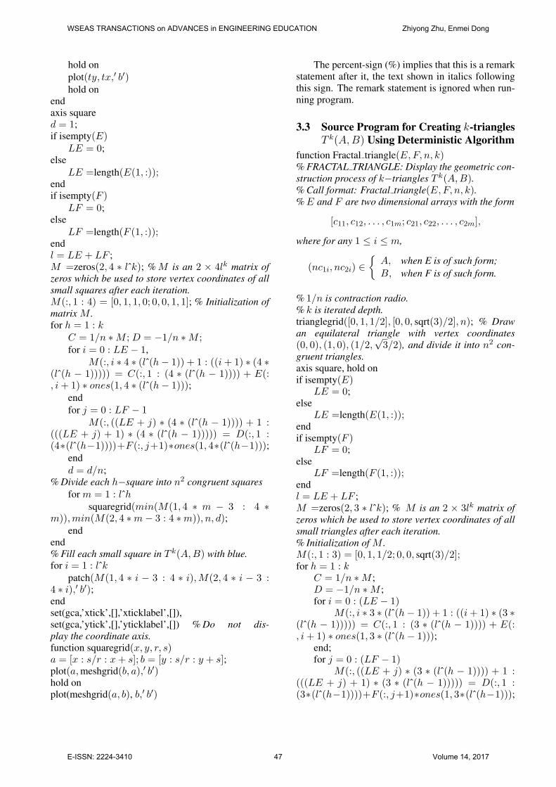
(a) The first step (b) The second step
(c) The third step (d) The fourth step
Figure 2: The first four steps of constructing GeneralSierpinski carpet T (A1, B1).
Example 1. Let n = 3,
A1 = (0, 0), (0, 2), (2, 1), B1 = (2, 2).
We can obtain the fine structures of the first four stepsof constructing General Sierpinski carpet T (A1, B1)by running the following instructions in turn:
Fractal square([0, 0, 2/3; 0, 2/3, 1/3], [2/3; 2/3], 3, k),
k = 1, 2, 3, 4,see Figure 2.
Example 2. Let n = 3,
A2 = {(1, 0), (12,
√3
2), (
32,
√3
2)},
B2 = (32,
√3
2), (
52,
√3
2), (2,
√3)}.
We can obtain the fine structures of the firstfour steps of constructing general Sierpinski gasketT (A2, B2) by running the instructions in turn: Frac-tal triangle(E, F, 3, k), where
E = [1/3, 1/6, 1/2; 0, sqrt(3)/6, sqrt(3)/6],
F = [1/2, 5/6, 2/3; sqrt(3)/6, sqrt(3)/6, sqrt(3)/3],
k = 1, 2, 3, 4,see Figure 3.
WSEAS TRANSACTIONS on ADVANCES in ENGINEERING EDUCATION Zhiyong Zhu, Enmei Dong
E-ISSN: 2224-3410 48 Volume 14, 2017
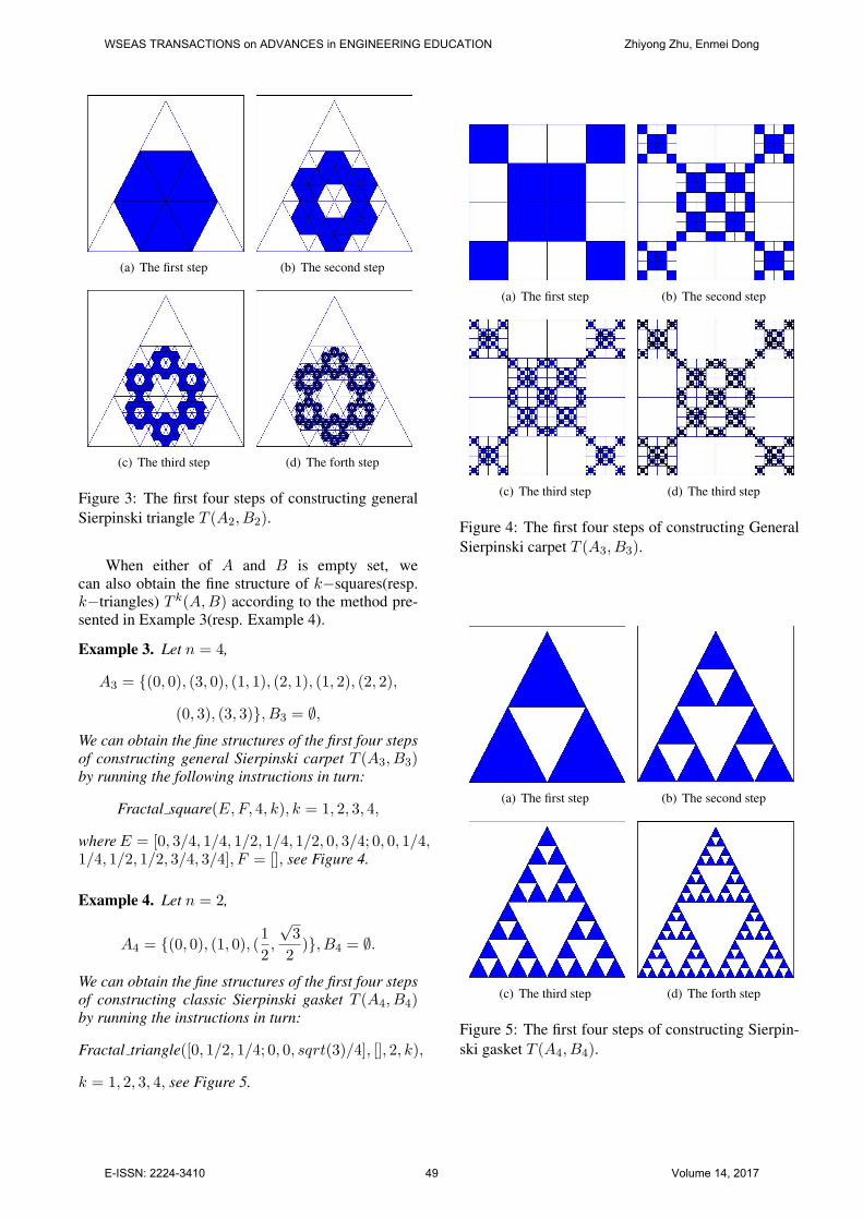
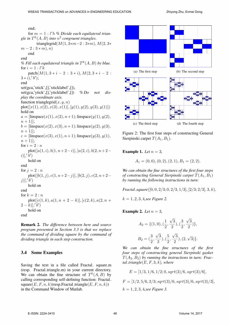
(a) The first step (b) The second step
(c) The third step (d) The forth step
Figure 3: The first four steps of constructing generalSierpinski triangle T (A2, B2).
When either of A and B is empty set, wecan also obtain the fine structure of k−squares(resp.k−triangles) T k(A,B) according to the method pre-sented in Example 3(resp. Example 4).
Example 3. Let n = 4,
A3 = {(0, 0), (3, 0), (1, 1), (2, 1), (1, 2), (2, 2),
(0, 3), (3, 3)}, B3 = ∅,We can obtain the fine structures of the first four stepsof constructing general Sierpinski carpet T (A3, B3)by running the following instructions in turn:
Fractal square(E, F, 4, k), k = 1, 2, 3, 4,
where E = [0, 3/4, 1/4, 1/2, 1/4, 1/2, 0, 3/4; 0, 0, 1/4,1/4, 1/2, 1/2, 3/4, 3/4], F = [], see Figure 4.
Example 4. Let n = 2,
A4 = {(0, 0), (1, 0), (12,
√3
2)}, B4 = ∅.
We can obtain the fine structures of the first four stepsof constructing classic Sierpinski gasket T (A4, B4)by running the instructions in turn:
Fractal triangle([0, 1/2, 1/4; 0, 0, sqrt(3)/4], [], 2, k),
k = 1, 2, 3, 4, see Figure 5.
(a) The first step (b) The second step
(c) The third step (d) The third step
Figure 4: The first four steps of constructing GeneralSierpinski carpet T (A3, B3).
(a) The first step (b) The second step
(c) The third step (d) The forth step
Figure 5: The first four steps of constructing Sierpin-ski gasket T (A4, B4).
WSEAS TRANSACTIONS on ADVANCES in ENGINEERING EDUCATION Zhiyong Zhu, Enmei Dong
E-ISSN: 2224-3410 49 Volume 14, 2017
Remark 3. Dividing each square(resp. equilateraltriangle) chosen in each step for generating T (A,B)into n2 congruent squares(resp. triangles) will behelpful for researcher to investigate deeper the con-nection between higher and lower k-squares (resp. k-triangles). We can make the grid not shown in the fig-ure by deleting the function of drawing grid in sourceprograms presented as above when we don’t wantgrid.
Remark 4. Our results in present paper include theresults in our previous paper [22].
4 Applying Random Iterated Algo-rithm to Generate General Sier-pinski Fractal
Applying random iterated algorithm to generate frac-tal, the principle is clear and simple, it is easy to im-plement in any programming language and the resultsit generates are very spectacular and may be used forany graphical goal, not only for mathematical reasons.The method may be illustrated with the Yuval Fishersspecial copyrighter(see [20]) which receives as entryan arbitrary image (may be a point) and applies toit the set of affine transformation, generating a newimage. The image obtained is transmitted, using afeedback process, on the entry of the copyrighter andthe process is repeated for several times. For exam-ple, consider that the transformations are those whichdescribe the Sierpinski gasket. If we test the YuvalFisher copyrighter for different initial images we canobserve that the final image is the same, so it not de-pends on the initial image but is defined by the affinetransforms applied to it. It is one of the most usedmethods of generating a self-similar fractals. For cre-ating T (A,B) using random iterated algorithm stepsgiven below should be considered.
Step 1: Choose (x, y) = (0, 0) as starting point.Step 2: Let (x1, y1) be the point obtained by ap-
plying a transformation in the IFS, where each trans-formation are chosen with probability 1/n.
Step 3: Repeat the step 2 with (x1, y1) as initialpoint.
Step 4: Repeat step 3 again and again, this step 3can be repeated infinite number of times.
4.1 Source Program for Creating T (A,B)Using Random Iterated Algorithm
function Sierpinskifractal (k, n,M,P )% SIERPINSKIFRACTAL: Drawing general Sierpin-ski carpet(resp. triangle) T (A,B) by random iteratedalgorithm.
% Call format: Sierpinskifractal (k, n,M,P ).% k is the number of iteration.% n is the number of affine transformations in IFS.% M = [a11, a12, · · · , a16; a21, a22, · · · , a26; · · · ,an1, an2, · · · , an6] is a n× 6 array, where
[ai1, ai2, · · · , ai6] = [ai, bi, ei, ci, di, fi]
satisfying (2).% P = (p1, p2, · · · , pn) is a dimension array with∑n
i=1 pi = 1.x = 0; y = 0; r =rand(1, k); B =zeros(2, k);w =zeros(1, n);w(1) = P (1);for i = 2 : n
w(i) = w(i− 1) + P (i);endm = 1;for i = 1 : k
for j = 1 : nif ri < w(j)
a = M(j, 1); b = M(j, 2); e =M(j, 3); c = M(j, 4); d = M(j, 5); f = M(j, 6);
break;end
endx = a ∗ x + b ∗ y + e; y = c ∗ x + d ∗ y + f ;B(1,m) = x; B(2,m) = y;m = m + 1;
endplot(B(1, :),B(2, :),’.’,’markersize’,0.5)set(gca,’xtick’,[],’xticklabel’,[]);set(gca,’ytick’,[],’yticklabel’,[])
4.2 Comments and Examples
Remark 5. We can’t obtain the fine structure ofk−squares(resp. k−triangles) by using random iter-ated algorithm. But we can obtain close approxima-tion of general Sierpinski carpet(resp. general Sier-pinski gasket) T (A,B) faster than using deterministicalgorithm and need lesser computer memory.
Remark 6. For facilitating the readers to observe andunderstand, one may add the command lines which di-vide [0, 1]2(resp. equilateral triangle) into n2 congru-ent ones (see source programs in Section 3 or [22] fordetail) at the beginning of program, the rest remainthe same.
Example 5. Let n = 5,
A5 = {(0, 0), (1, 0), ((2, 0))}, B5 = {(2, 2), (2, 3)}.We can obtain close approximation of general Sierpin-ski carpet T (A5, B5) by calling the function: fractal(k, 5,M, P ) in the Matlab command window prompt,as shown in Figure 6. Table 1 lists correspondingtransformations.
WSEAS TRANSACTIONS on ADVANCES in ENGINEERING EDUCATION Zhiyong Zhu, Enmei Dong
E-ISSN: 2224-3410 50 Volume 14, 2017
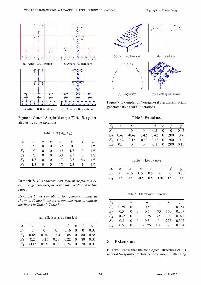
(a) After 1000 iterations (b) After 5000 iterations
(c) After 10000 iterations (d) After 50000 iterations
Figure 6: General Sierpinski carpet T (A5, B5) gener-ated using some iterations.
Table 1: T (A5, B5)
Si a b c d e f p
S1 1/3 0 0 1/3 0 0 1/5S2 1/3 0 0 1/3 1/3 0 1/5S3 1/3 0 0 1/3 2/3 0 1/5S4 -1/3 0 0 -1/3 2/3 2/3 1/5S5 -1/3 0 0 -1/3 2/3 1 1/5
Remark 7. This program can draw more fractals ex-cept the general Sierpinski fractals mentioned in thispaper.
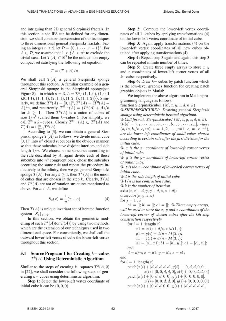
Example 6. We can obtain four famous fractals asshown in Figure 7, the corresponding transformationsare listed in Table 2-Table 5.
Table 2: Bernsley fern leaf
Si a b c d e f p
S1 0 0 0 0.16 0 0 0.01S2 0.85 0.04 -0.04 0.85 0 80 0.85S3 0.2 -0.26 0.23 0.22 0 80 0.07S4 -0.15 0.28 0.26 0.24 0 20 0.07
(a) Bernsley fern leaf (b) Fractal tree
(c) Levy curve (d) Flamboyrent crown
Figure 7: Examples of Non-general Sierpinski fractalsgenerated using 50000 iterations
Table 3: Fractal tree
Si a b c d e f p
S1 0 0 0 0.5 0 0 0.05S2 0.42 -0.42 0.42 0.42 0 200 0.4S3 0.42 0.42 -0.42 0.42 0 200 0.4S4 0.1 0 0 0.1 0 200 0.15
Table 4: Levy curve
Si a b c d e f p
S1 0.5 -0.5 0.5 0.5 0 0 0.05S2 0.5 0.5 -0.5 0.5 150 150 0.5
Table 5: Flamboyrent crown
Si a b c d e f p
S1 0.25 0 0 0.5 0 0 0.154S2 0.5 0 0 0.5 -75 150 0.307S3 -0.25 0 0 -0.25 75 300 0.078S4 0.5 0 0 0.5 0 225 0.307S5 0.5 0 0 -0.25 150 375 0.154
5 Extension
It is well know that the topological structures of 3Dgeneral Sierpinski fractals become more challenging
WSEAS TRANSACTIONS on ADVANCES in ENGINEERING EDUCATION Zhiyong Zhu, Enmei Dong
E-ISSN: 2224-3410 51 Volume 14, 2017
and intriguing than 2D general Sierpinski fractals. Inthis section, since IFS can be defined for any dimen-sion, we shall consider the extension of our techniquesto three dimensional general Sierpinski fractals. Fix-ing an integer n ≥ 2, let D = {0, 1, · · · , n− 1}3. ForA ⊂ D, we assume that 1 < ]A < n3 to exclude thetrivial case. Let T (A) ⊂ R3 be the unique non-emptycompact set satisfying the following set equation:
T = (T + A)/n.
We shall call T (A) a general Sierpinski spongethroughout this section. A familiar example of a gen-eral Sierpinski sponge is the Sierpinski sponge(seeFigure 8), in which n = 3, A = D\{(1, 1, 0), (1, 0, 1),(0,1,1), (1, 1, 1), (2, 1, 1), (1, 2, 1), (1, 1, 2)}}. Simi-larly, we define T 0(A) = [0, 1]3, T 1(A) = (T 0(A) +A)/n, and recurrently, T k+1(A) = (T k(A) + A)/nfor k ≥ 1. Then T k(A) is a union of cubes ofsize 1/nk (called them k−cubes ). For simplify, wecall T k a k−cubes. Clearly T k+1(A) ⊂ T k(A) andT (A) = ∩∞k=1T
k(A).According to [3], we can obtain a general Sier-
pinski sponge T (A) as follows: we divide initial cube[0, 1]3 into n3 closed subcubes in the obvious manner,so that these subcubes have disjoint interiors and sidelength 1/n. We choose some subcubes according tothe rule described by A, again divide each of thesesubcubes into n3 congruent ones, chose the subcubesaccording the same rule and repeat the procedure in-ductively to the infinity, then we get general Sierpinskisponge T (A). For any k ≥ 1, then T k(A) is the unionof cubes that are chosen in the step k. Clearly, T (A)and T k(A) are not of rotation structures mentioned asabove. For a ∈ A, we define
Sa(x) =1n
(x + a). (4)
Then T (A) is unique invariant set of iterated functionsystem {Sa}a∈A.
In this section, we obtain the geometric mod-elling of such T k(A)(or T (A)) by using two methods,which are the extension of our techniques used in twodimensional space. For conveniently, we shall call theoutward lower-left vertex of cube the lower-left vertexthroughout this section.
5.1 Source Program 1 for Creating k− cubesT k(A) Using Deterministic Algorithm
Similar to the steps of creating k−squares T k(A, ∅)in [22], we shall consider the following steps of gen-erating k− cubes using deterministic algorithm.
Step 1: Select the lower-left vertex coordinate ofinitial cube it can be (0, 0, 0).
Step 2: Compute the lower-left vertex coordi-nates of all 1−cubes by applying transformations (4)on the lower-left vertex coordinate of initial cube.
Step 3: Again apply transformations (4) on thelower-left vertex coordinates of all new cubes ob-tained after applying transformations (4).
Step 4: Repeat step 3 again and again, this step 3can be repeated infinite number of times.
Step 5: Create three empty arrays to store x, yand z coordinates of lower-left corner vertex of allk−cubes respectively.
Step 6: Draw k− cubes by patch function whichis the low-level graphics function for creating patchgraphics objects in Matlab.
We implement the above algorithm in Matlab pro-gramming language as follows:function Sierpinskicube1 (M, x, y, z, d, n, k)% SIERPINSKICUBE1: Drawing general Sierpinskisponge using deterministic iterated algorithm.% Call format: Sierpinskicube1 (M, x, y, z, d, n, k).% M = [a1, · · · , am; b1, · · · , bm; c1, · · · , cm], where(ai/n, bi/n, ci/n), i = 1, 2, · · · ,m(1 < m < n3),are the lower-left coordinates of small cubes chosenaccording to certain rule after the first division for theinitial cube.% x is the x−coordinate of lower-left corner vertexof initial cube.% y is the y−coordinate of lower-left corner vertexof initial cube.% z is the z−coordinate of lower-left corner vertex ofinitial cube.% d is the side length of initial cube.% 1/n is the contraction ratio.% k is the number of iteration.axis([x, x + d, y, y + d, z, z + d])drawcube(x, y, z, d)for j = 1 : k
a1 = []; b1 = []; c1 = []; % Three empty arrays,will be used to store the x, y and z coordinates of thelower-left corner of chosen cubes after the kth stepconstruction respectively.
for i = 1 :length(x)x1 = x(i) + d/n ∗M(1, :);y1 = y(i) + d/n ∗M(2, :);z1 = z(i) + d/n ∗M(3, :);a1 = [a1, x1]; b1 = [b1, y1]; c1 = [c1, z1];
endd = d/n; x = a1; y = b1; z = c1;
endfor i = 1 :length(x)
patch(x(i) + [d, d, d, d, d], y(i) + [0, d, d, 0, 0],z(i)+[0, 0, d, d, 0], z(i)+[0, 0, d, d, 0])
patch(x(i) + [0, d, d, 0, 0], y(i) + [0, 0, 0, 0, 0],z(i)+[0, 0, d, d, 0], y(i)+[0, 0, 0, 0, 0])
patch(x(i) + [0, d, d, 0, 0], y(i) + [d, d, d, d, d],
WSEAS TRANSACTIONS on ADVANCES in ENGINEERING EDUCATION Zhiyong Zhu, Enmei Dong
E-ISSN: 2224-3410 52 Volume 14, 2017
z(i)+[0, 0, d, d, 0], x(i)+[0, d, d, 0, 0])patch(x(i) + [0, d, d, 0, 0], y(i) + [0, 0, d, d, 0],
z(i)+[0, 0, 0, 0, 0], y(i)+[0, 0, d, d, 0])patch(x(i) + [0, d, d, 0, 0], y(i) + [0, 0, d, d, 0],
z(i)+[d, d, d, d, d], x(i)+[0, 0, 0, 0, 0])patch(x(i) + [0, 0, 0, 0, 0], y(i) + [0, d, d, 0, 0],
z(i)+[0, 0, d, d, 0], z(i)+[0, 0, d, d, 0])endaxis equalaxis offset(gcf,’color’,[1, 1, 1])function drawcube(x, y, z, d)u =([0 1 1 0 0 0;1 1 0 0 1 1;1 1 0 0 1 1;0 1 1 0 00])∗d + x(1);v =([0 0 1 1 0 0;0 1 1 0 0 0;0 1 1 0 1 1;0 0 1 1 11])∗d + y(1);w =([0 0 0 0 0 1;0 0 0 0 0 1;1 1 1 1 0 1;1 1 1 1 01])∗d + z(1);for i = 1 : 6
h =patch(u(:, i), v(:, i), w(:, i),’w’);set(h,’edgecolor’,’k’,’facealpha’,0.5)
endh=gcf;view(-33,18)
Example 7. Let n = 3,
A1 = {(0, 0, 0), (13, 0, 0), (
23, 0, 0), (0,
13, 0)
(23,13, 0), (0,
23, 0), (
13,23, 0), (
23,23, 0)
(0, 0,13), (
23, 0,
13), (0,
23,13), (
23,23,13)
(0, 0,23), (
13, 0,
23), (
23, 0,
23), (0,
13,23)
(23,13,23), (0,
23,23), (
13,23,23), (
23,23,23)}
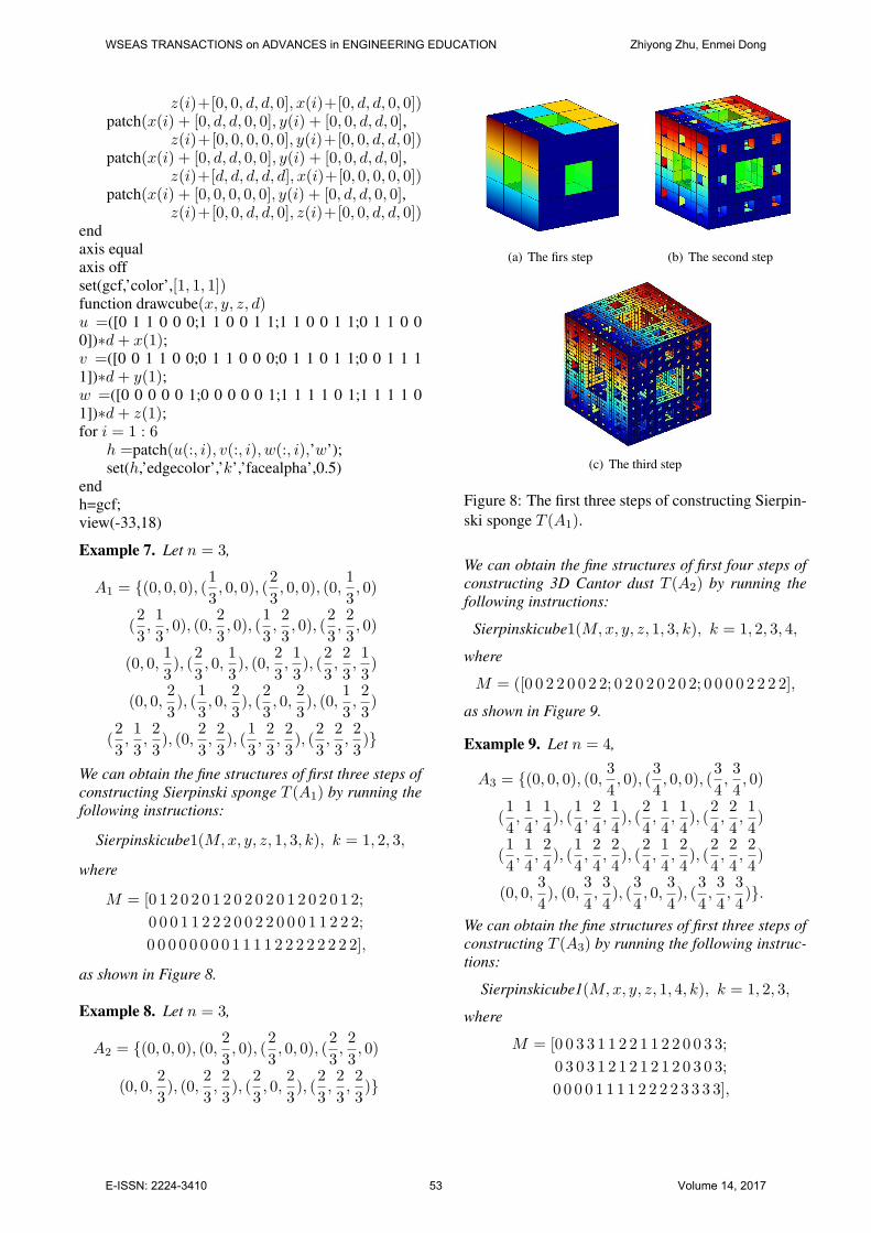
We can obtain the fine structures of first three steps ofconstructing Sierpinski sponge T (A1) by running thefollowing instructions:
Sierpinskicube1(M, x, y, z, 1, 3, k), k = 1, 2, 3,
where
M = [0 1 2 0 2 0 1 2 0 2 0 2 0 1 2 0 2 0 1 2;0 0 0 1 1 2 2 2 0 0 2 2 0 0 0 1 1 2 2 2;0 0 0 0 0 0 0 0 1 1 1 1 2 2 2 2 2 2 2 2],
as shown in Figure 8.
Example 8. Let n = 3,
A2 = {(0, 0, 0), (0,23, 0), (
23, 0, 0), (
23,23, 0)
(0, 0,23), (0,
23,23), (
23, 0,
23), (
23,23,23)}
(a) The firs step (b) The second step
(c) The third step
Figure 8: The first three steps of constructing Sierpin-ski sponge T (A1).
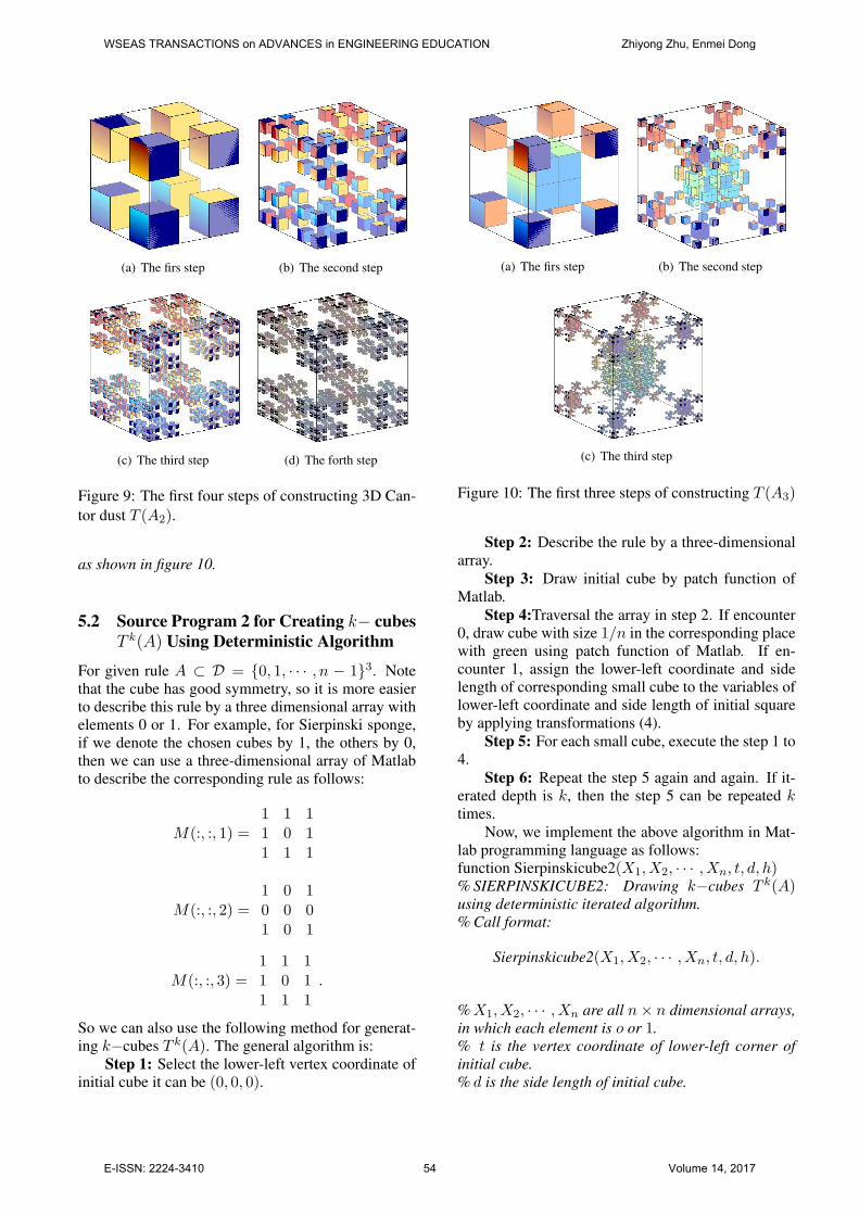
We can obtain the fine structures of first four steps ofconstructing 3D Cantor dust T (A2) by running thefollowing instructions:
Sierpinskicube1(M, x, y, z, 1, 3, k), k = 1, 2, 3, 4,
where
M = ([0 0 2 2 0 0 2 2; 0 2 0 2 0 2 0 2; 0 0 0 0 2 2 2 2],
as shown in Figure 9.
Example 9. Let n = 4,
A3 = {(0, 0, 0), (0,34, 0), (
34, 0, 0), (
34,34, 0)
(14,14,14), (
14,24,14), (
24,14,14), (
24,24,14)
(14,14,24), (
14,24,24), (
24,14,24), (
24,24,24)
(0, 0,34), (0,
34,34), (
34, 0,
34), (
34,34,34)}.
We can obtain the fine structures of first three steps ofconstructing T (A3) by running the following instruc-tions:
Sierpinskicube1(M, x, y, z, 1, 4, k), k = 1, 2, 3,
where
M = [0 0 3 3 1 1 2 2 1 1 2 2 0 0 3 3;0 3 0 3 1 2 1 2 1 2 1 2 0 3 0 3;0 0 0 0 1 1 1 1 2 2 2 2 3 3 3 3],
WSEAS TRANSACTIONS on ADVANCES in ENGINEERING EDUCATION Zhiyong Zhu, Enmei Dong
E-ISSN: 2224-3410 53 Volume 14, 2017
(a) The firs step (b) The second step
(c) The third step (d) The forth step
Figure 9: The first four steps of constructing 3D Can-tor dust T (A2).
as shown in figure 10.
5.2 Source Program 2 for Creating k− cubesT k(A) Using Deterministic Algorithm
For given rule A ⊂ D = {0, 1, · · · , n − 1}3. Notethat the cube has good symmetry, so it is more easierto describe this rule by a three dimensional array withelements 0 or 1. For example, for Sierpinski sponge,if we denote the chosen cubes by 1, the others by 0,then we can use a three-dimensional array of Matlabto describe the corresponding rule as follows:
M(:, :, 1) =1 1 11 0 11 1 1
M(:, :, 2) =1 0 10 0 01 0 1
M(:, :, 3) =1 1 11 0 11 1 1
.
So we can also use the following method for generat-ing k−cubes T k(A). The general algorithm is:
Step 1: Select the lower-left vertex coordinate ofinitial cube it can be (0, 0, 0).
(a) The firs step (b) The second step
(c) The third step
Figure 10: The first three steps of constructing T (A3)
Step 2: Describe the rule by a three-dimensionalarray.
Step 3: Draw initial cube by patch function ofMatlab.
Step 4:Traversal the array in step 2. If encounter0, draw cube with size 1/n in the corresponding placewith green using patch function of Matlab. If en-counter 1, assign the lower-left coordinate and sidelength of corresponding small cube to the variables oflower-left coordinate and side length of initial squareby applying transformations (4).
Step 5: For each small cube, execute the step 1 to4.
Step 6: Repeat the step 5 again and again. If it-erated depth is k, then the step 5 can be repeated ktimes.
Now, we implement the above algorithm in Mat-lab programming language as follows:function Sierpinskicube2(X1, X2, · · · , Xn, t, d, h)% SIERPINSKICUBE2: Drawing k−cubes T k(A)using deterministic iterated algorithm.% Call format:
Sierpinskicube2(X1, X2, · · · , Xn, t, d, h).
% X1, X2, · · · , Xn are all n× n dimensional arrays,in which each element is o or 1.% t is the vertex coordinate of lower-left corner ofinitial cube.% d is the side length of initial cube.
WSEAS TRANSACTIONS on ADVANCES in ENGINEERING EDUCATION Zhiyong Zhu, Enmei Dong
E-ISSN: 2224-3410 54 Volume 14, 2017
% h is the iterated depth.M =cat(3, X1, X2, · · · , Xn);u = t(1);v = t(2);w = t(3);l = d;if h == 0
returnendaxis([u, u + l, v, v + l, w, w + l])drawwhite(t,d)m =length(M);for i = 1 : m
for j = 1 : mfor k = 1 : m
if M(i, j, k) == 0drawcube([t(1) + d ∗ (k −
1)/m, t(2)+d∗(j−1)/m, t(3)+d∗(i−1)/m], d/m)else
Sierpinskicube2(X1, X2, · · · , Xn, [t(1)+d ∗ (k − 1)/m, t(2) + d ∗ (j − 1)/m, t(3) + d ∗ (i−1)/m], d/m, h− 1)
endend
endendaxis equalaxis offfunction drawcube(t, d)x =([0 1 1 0 0 0;1 1 0 0 1 1;1 1 0 0 1 1;0 1 1 0 00])∗d + t(1);y =([0 0 1 1 0 0;0 1 1 0 0 0;0 1 1 0 1 1;0 0 1 1 11])∗d + t(2);z =([0 0 0 0 0 1;0 0 0 0 0 1;1 1 1 1 0 1;1 1 1 1 01])∗d + t(3);for i = 1 : 6
s =patch(x(:, i), y(:, i), z(:, i),’g’);set(s,′ edgecolor′,′k′,′ facealpha′, 0.5)
ends =gcf;view(−33, 18)function drawwhite(t, d)x =([0 1 1 0 0 0;1 1 0 0 1 1;1 1 0 0 1 1;0 1 1 0 00])∗d + t(1);y =([0 0 1 1 0 0;0 1 1 0 0 0;0 1 1 0 1 1;0 0 1 1 11])∗d + t(2);z =([0 0 0 0 0 1;0 0 0 0 0 1;1 1 1 1 0 1;1 1 1 1 01])∗d + t(3);for i = 1 : 6
s =patch(x(:, i), y(:, i), z(:, i),’w’);set(s,’edgecolor’,’k’,’facealpha’,0.5)
ends =gcf;view(−33, 18)
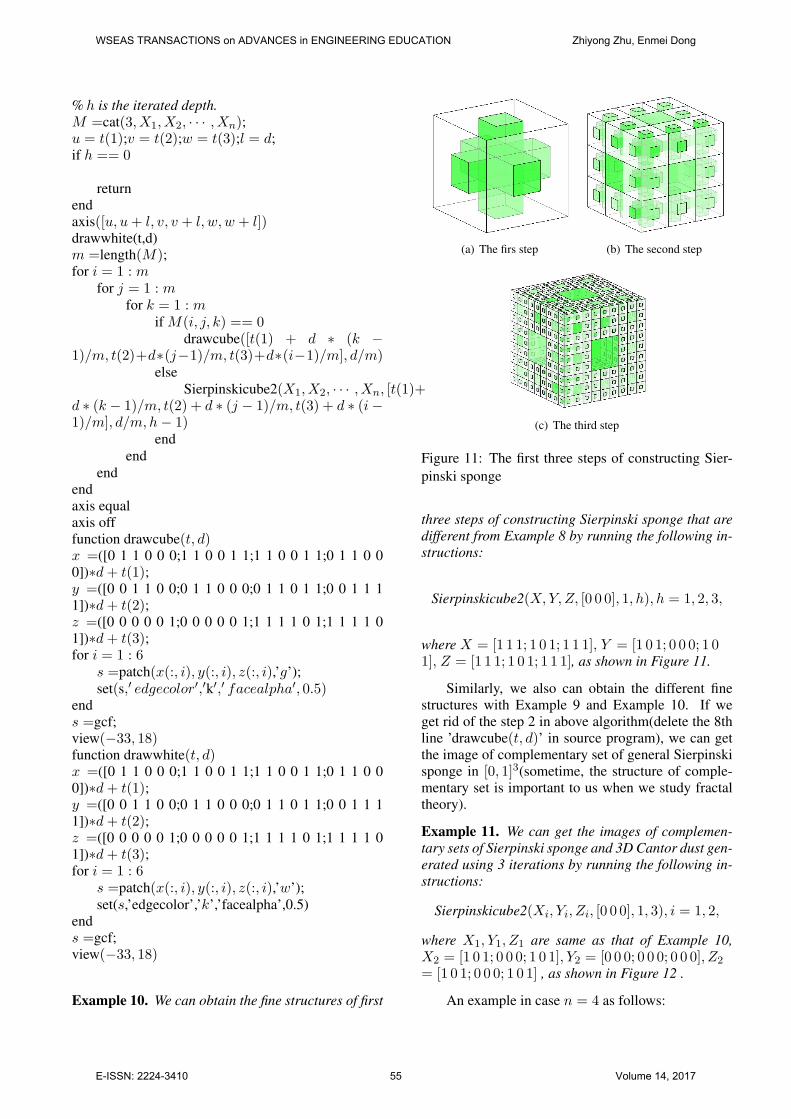
Example 10. We can obtain the fine structures of first
(a) The firs step (b) The second step
(c) The third step
Figure 11: The first three steps of constructing Sier-pinski sponge
three steps of constructing Sierpinski sponge that aredifferent from Example 8 by running the following in-structions:
Sierpinskicube2(X, Y, Z, [0 0 0], 1, h), h = 1, 2, 3,
where X = [1 1 1; 1 0 1; 1 1 1], Y = [1 0 1; 0 0 0; 1 01], Z = [1 1 1; 1 0 1; 1 1 1], as shown in Figure 11.
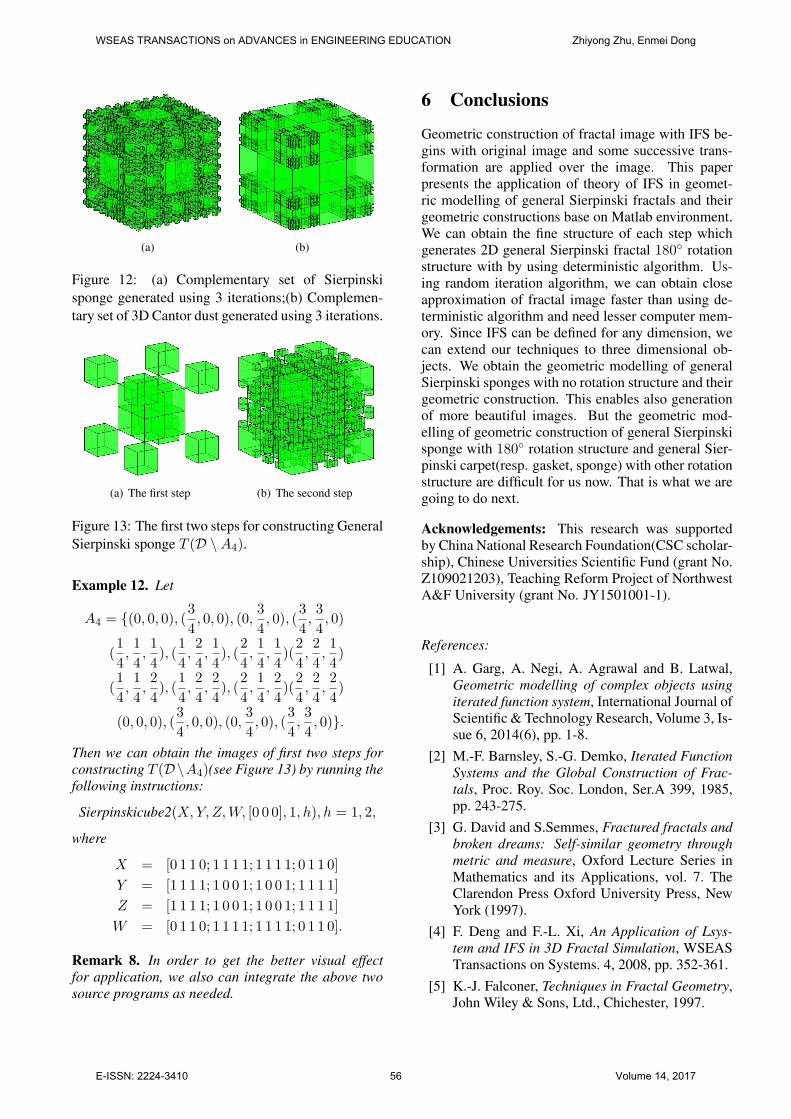
Similarly, we also can obtain the different finestructures with Example 9 and Example 10. If weget rid of the step 2 in above algorithm(delete the 8thline ’drawcube(t, d)’ in source program), we can getthe image of complementary set of general Sierpinskisponge in [0, 1]3(sometime, the structure of comple-mentary set is important to us when we study fractaltheory).
Example 11. We can get the images of complemen-tary sets of Sierpinski sponge and 3D Cantor dust gen-erated using 3 iterations by running the following in-structions:
Sierpinskicube2(Xi, Yi, Zi, [0 0 0], 1, 3), i = 1, 2,
where X1, Y1, Z1 are same as that of Example 10,X2 = [1 0 1; 0 0 0; 1 0 1], Y2 = [0 0 0; 0 0 0; 0 0 0], Z2
= [1 0 1; 0 0 0; 1 0 1] , as shown in Figure 12 .
An example in case n = 4 as follows:
WSEAS TRANSACTIONS on ADVANCES in ENGINEERING EDUCATION Zhiyong Zhu, Enmei Dong
E-ISSN: 2224-3410 55 Volume 14, 2017
(a) (b)
Figure 12: (a) Complementary set of Sierpinskisponge generated using 3 iterations;(b) Complemen-tary set of 3D Cantor dust generated using 3 iterations.
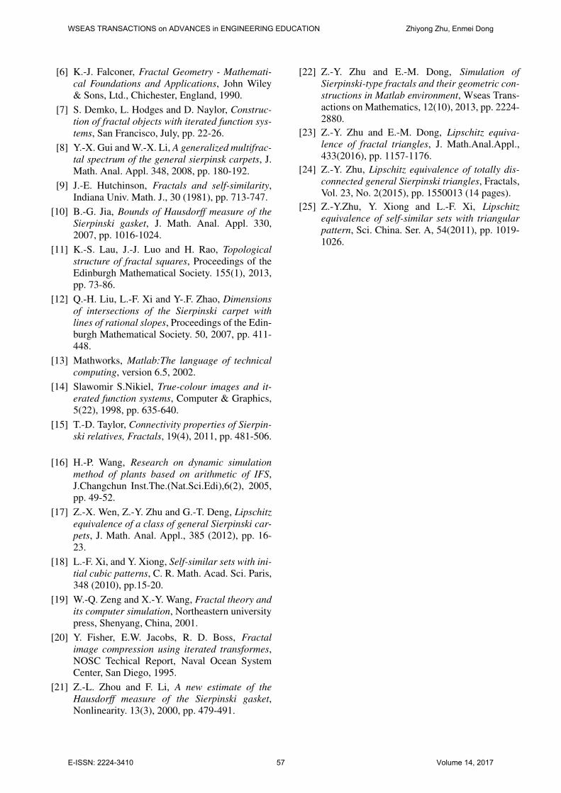
(a) The first step (b) The second step
Figure 13: The first two steps for constructing GeneralSierpinski sponge T (D \A4).
Example 12. Let
A4 = {(0, 0, 0), (34, 0, 0), (0,
34, 0), (
34,34, 0)
(14,14,14), (
14,24,14), (
24,14,14)(
24,24,14)
(14,14,24), (
14,24,24), (
24,14,24)(
24,24,24)
(0, 0, 0), (34, 0, 0), (0,
34, 0), (
34,34, 0)}.
Then we can obtain the images of first two steps forconstructing T (D\A4)(see Figure 13) by running thefollowing instructions:
Sierpinskicube2(X, Y, Z, W, [0 0 0], 1, h), h = 1, 2,
where
X = [0 1 1 0; 1 1 1 1; 1 1 1 1; 0 1 1 0]Y = [1 1 1 1; 1 0 0 1; 1 0 0 1; 1 1 1 1]Z = [1 1 1 1; 1 0 0 1; 1 0 0 1; 1 1 1 1]W = [0 1 1 0; 1 1 1 1; 1 1 1 1; 0 1 1 0].
Remark 8. In order to get the better visual effectfor application, we also can integrate the above twosource programs as needed.
6 Conclusions
Geometric construction of fractal image with IFS be-gins with original image and some successive trans-formation are applied over the image. This paperpresents the application of theory of IFS in geomet-ric modelling of general Sierpinski fractals and theirgeometric constructions base on Matlab environment.We can obtain the fine structure of each step whichgenerates 2D general Sierpinski fractal 180◦ rotationstructure with by using deterministic algorithm. Us-ing random iteration algorithm, we can obtain closeapproximation of fractal image faster than using de-terministic algorithm and need lesser computer mem-ory. Since IFS can be defined for any dimension, wecan extend our techniques to three dimensional ob-jects. We obtain the geometric modelling of generalSierpinski sponges with no rotation structure and theirgeometric construction. This enables also generationof more beautiful images. But the geometric mod-elling of geometric construction of general Sierpinskisponge with 180◦ rotation structure and general Sier-pinski carpet(resp. gasket, sponge) with other rotationstructure are difficult for us now. That is what we aregoing to do next.
Acknowledgements: This research was supportedby China National Research Foundation(CSC scholar-ship), Chinese Universities Scientific Fund (grant No.Z109021203), Teaching Reform Project of NorthwestA&F University (grant No. JY1501001-1).
References:
[1] A. Garg, A. Negi, A. Agrawal and B. Latwal,Geometric modelling of complex objects usingiterated function system, International Journal ofScientific & Technology Research, Volume 3, Is-sue 6, 2014(6), pp. 1-8.
[2] M.-F. Barnsley, S.-G. Demko, Iterated FunctionSystems and the Global Construction of Frac-tals, Proc. Roy. Soc. London, Ser.A 399, 1985,pp. 243-275.
[3] G. David and S.Semmes, Fractured fractals andbroken dreams: Self-similar geometry throughmetric and measure, Oxford Lecture Series inMathematics and its Applications, vol. 7. TheClarendon Press Oxford University Press, NewYork (1997).
[4] F. Deng and F.-L. Xi, An Application of Lsys-tem and IFS in 3D Fractal Simulation, WSEASTransactions on Systems. 4, 2008, pp. 352-361.
[5] K.-J. Falconer, Techniques in Fractal Geometry,John Wiley & Sons, Ltd., Chichester, 1997.
WSEAS TRANSACTIONS on ADVANCES in ENGINEERING EDUCATION Zhiyong Zhu, Enmei Dong
E-ISSN: 2224-3410 56 Volume 14, 2017
[6] K.-J. Falconer, Fractal Geometry - Mathemati-cal Foundations and Applications, John Wiley& Sons, Ltd., Chichester, England, 1990.
[7] S. Demko, L. Hodges and D. Naylor, Construc-tion of fractal objects with iterated function sys-tems, San Francisco, July, pp. 22-26.
[8] Y.-X. Gui and W.-X. Li, A generalized multifrac-tal spectrum of the general sierpinsk carpets, J.Math. Anal. Appl. 348, 2008, pp. 180-192.
[9] J.-E. Hutchinson, Fractals and self-similarity,Indiana Univ. Math. J., 30 (1981), pp. 713-747.
[10] B.-G. Jia, Bounds of Hausdorff measure of theSierpinski gasket, J. Math. Anal. Appl. 330,2007, pp. 1016-1024.
[11] K.-S. Lau, J.-J. Luo and H. Rao, Topologicalstructure of fractal squares, Proceedings of theEdinburgh Mathematical Society. 155(1), 2013,pp. 73-86.
[12] Q.-H. Liu, L.-F. Xi and Y-.F. Zhao, Dimensionsof intersections of the Sierpinski carpet withlines of rational slopes, Proceedings of the Edin-burgh Mathematical Society. 50, 2007, pp. 411-448.
[13] Mathworks, Matlab:The language of technicalcomputing, version 6.5, 2002.
[14] Slawomir S.Nikiel, True-colour images and it-erated function systems, Computer & Graphics,5(22), 1998, pp. 635-640.
[15] T.-D. Taylor, Connectivity properties of Sierpin-ski relatives, Fractals, 19(4), 2011, pp. 481-506.
[16] H.-P. Wang, Research on dynamic simulationmethod of plants based on arithmetic of IFS,J.Changchun Inst.The.(Nat.Sci.Edi),6(2), 2005,pp. 49-52.
[17] Z.-X. Wen, Z.-Y. Zhu and G.-T. Deng, Lipschitzequivalence of a class of general Sierpinski car-pets, J. Math. Anal. Appl., 385 (2012), pp. 16-23.
[18] L.-F. Xi, and Y. Xiong, Self-similar sets with ini-tial cubic patterns, C. R. Math. Acad. Sci. Paris,348 (2010), pp.15-20.
[19] W.-Q. Zeng and X.-Y. Wang, Fractal theory andits computer simulation, Northeastern universitypress, Shenyang, China, 2001.
[20] Y. Fisher, E.W. Jacobs, R. D. Boss, Fractalimage compression using iterated transformes,NOSC Techical Report, Naval Ocean SystemCenter, San Diego, 1995.
[21] Z.-L. Zhou and F. Li, A new estimate of theHausdorff measure of the Sierpinski gasket,Nonlinearity. 13(3), 2000, pp. 479-491.
[22] Z.-Y. Zhu and E.-M. Dong, Simulation ofSierpinski-type fractals and their geometric con-structions in Matlab environment, Wseas Trans-actions on Mathematics, 12(10), 2013, pp. 2224-2880.
[23] Z.-Y. Zhu and E.-M. Dong, Lipschitz equiva-lence of fractal triangles, J. Math.Anal.Appl.,433(2016), pp. 1157-1176.
[24] Z.-Y. Zhu, Lipschitz equivalence of totally dis-connected general Sierpinski triangles, Fractals,Vol. 23, No. 2(2015), pp. 1550013 (14 pages).
[25] Z.-Y.Zhu, Y. Xiong and L.-F. Xi, Lipschitzequivalence of self-similar sets with triangularpattern, Sci. China. Ser. A, 54(2011), pp. 1019-1026.
WSEAS TRANSACTIONS on ADVANCES in ENGINEERING EDUCATION Zhiyong Zhu, Enmei Dong
E-ISSN: 2224-3410 57 Volume 14, 2017