Pitfalls in prestack inversion of merged seismic surveys

Sumit Verma1, Yoryenys Del Moro2, and Kurt J. Marfurt1

Abstract

Modern 3D seismic surveys are often of such good quality and 3D interpretation packages so user-friendlythat seismic interpretation is no longer exclusively carried out by geophysicists. This ease-of-use has also beenextended to more quantitative workflows, such as 3D prestack inversion, putting it in the hands of the “non-expert” — be it geologist, engineer, or new-hire geophysicist. Indeed, given good quality input seismicdata, almost any interpreter who can generate good well ties and define an accurate background model ofP-impedance, S-impedance, and density can generate a quality prestack inversion. Two of the authors arenew geophysicists who fell into the prestack inversion “pit.” Fortunately, they were able to recognize that some-thing was wrong. We applied prestack inversion to gathers that were carefully reprocessed by a major servicecompany. The problem, however, was not with the processing, but with our lack of understanding of the inputlegacy data that formed part of a larger “megamerge” survey. Not all of the surveys that were merged had thesame offset range. In the migration step, gaps in long offsets of the older surveys were not muted. Migrationnoise from newer surveys was allowed to fill this space. We share our initial workflow and suspicious results.We also clarify the meaning of “fold” and “offset” for prestack-migrated gathers. In addition to presenting someQC tools useful in analyzing megamerge surveys, we show how, by limiting the offsets used in our prestackinversion, we obtain less aggressive but still useful results.

IntroductionMuch of the midcontinental USA, including Texas, is

covered by legacy 3D seismic surveys. During theperiod of low oil prices in 1980s and 1990s, many ofthese properties were sold, traded, or consolidated,while licenses to the 3D surveys were in turn tradedto data brokers in exchange for seismic data over areasof more active interest. Most data brokers (some ofwhom are major service companies as in this study)pride themselves in their ability to pull more infor-mation out of legacy data. They do this in two ways.First, they reprocess the data using modern surface-consistent statics, noise-reduction, spectral balancing,and seismic imaging techniques. Second, they mergethe prestack data with adjacent surveys, thereby in-creasing the migration aperture, resulting in improvedlateral resolution of steeply dipping faults, channeledges, and other discontinuities, particularly near theinternal edges of the surveys that form the megamerge.Such processing can be difficult.

The megamerge survey discussed in this paper wasacquired with dynamite in some areas, and vibroseiswith different sweeps and number of vibrators in otherparts of the survey. The geophones may be grouped

in different arrays and may have different spectralresponses. It is common for the shot and receiver linespacing and also for the line orientations to changefrom survey to survey. Nevertheless, careful processingcan produce significantly improved results. Using thestacked version of the data discussed here, Del Moroet al. (2013) illustrate the improvements of the mega-merge versus a unmerged legacy survey in mappingincised Pennsylvanian age Red Fork channels usingseismic attributes.

The advent of shale, tight sand, tight lime, and otherresource plays has renewed interest in these legacy sur-veys. Most resource plays are exploited through hori-zontal drilling followed by either hydraulic fracturing,acidation, or both. In addition to identifying horizontaldrilling hazards (geohazards), we wish to better quan-tify the geomechanical properties (for hydraulic fractur-ing) and lithology (for higher porosity sweet spots)through the use of prestack impedance inversion.

The survey of interest was shot at various times, be-ginning in the mid-1990s. CGGVeritas acquired licensesfor these surveys, shot infill data where necessary,and carefully reprocessed them, resulting in a mega-merge survey (Figure 1). Many of these surveys were

1University of Oklahoma, ConocoPhillips School of Geology and Geophysics, Norman, Oklahoma, USA. E-mail: sumit.verma@ou.edu; kmarfurt@ou.edu.

2Noble Energy, Houston, Texas, USA. E-mail: yoryenysdelmoro@gmail.com.Manuscript received by the Editor 1 March 2013; revised manuscript received 24 April 2013; published online 2 August 2013. This paper appears

in INTERPRETATION, Vol. 1, No. 1 (August 2013); p. A1–A9, 10 FIGS.http://dx.doi.org/10.1190/INT-2013-0024.1. © 2013 Society of Exploration Geophysicists and American Association of Petroleum Geologists. All rights reserved.

t

Pitfalls

Interpretation / August 2013 A1

Dow

nloa

ded

08/2

3/13

to 1

29.1

5.12

7.24

5. R

edis

trib

utio

n su

bjec

t to

SEG

lice

nse

or c

opyr

ight

; see

Ter

ms

of U

se a

t http

://lib

rary

.seg

.org

/

shot to map Pennsylvanian-age Red Fork sandstones.Although the Red Fork is the focus of this paper, themajor focus of most of the operators is now on thedeeper Mississippian-age Woodford Shale, MississippiLime, and Hunton Limestone resource plays (Figure 2).

We encountered a pitfall while attempting prestackimpedance inversion of the megamerge survey. Thedata were very carefully reprocessed, with most of theevents quite flat and relatively noise free on commonreflection point gathers. Our objective was to use pre-stack inversion to identify what are known as “invisible”Red Fork sands — sands that are not seen on conven-tional stacked or P-impedance seismic data volumeswhere polarity reversals give rise to a low-amplitudestack. Such sands are commonly logged while drillingfor deeper Woodford Shale objectives. Barber and Mar-furt (2010) applied fluid substitution to such wells in aneighboring county and similar megamerge survey, andhypothesized that there should be a shear impedanceanomaly if the data could be processed using prestackinversion.

We begin with data description and follow up with anoverview of the assumptions required by prestackinversion. Next, we briefly review prestack migration,explaining the meaning of offset and fold on common-offset migrated results. This background allows us to dis-cuss the pitfall that befell us. We show the suspicious

Figure 1. Location map of Anadarko basin area on map ofOklahoma, and location of study area in Anadarko basinmarked by green boundary (modified from Northcutt andCampbell, 1988).

Figure 2. Stratigraphy of Anadarko basin in Pennsylvanian and Mississippian age, here Red Fork Formation and two of the geo-logic formations that appear as strong reflectors on seismic are highlighted in pink. Hunton (highlighted in blue) and Woodford(highlighted with green) are also formation of interest for current operators in the area (Modified from Clement, 1991).

A2 Interpretation / August 2013

Dow

nloa

ded

08/2

3/13

to 1

29.1

5.12

7.24

5. R

edis

trib

utio

n su

bjec

t to

SEG

lice

nse

or c

opyr

ight

; see

Ter

ms

of U

se a

t http

://lib

rary

.seg

.org

/

results, and follow with some simple quality controlplots and representative CRP gathers that illustratewhat happened. With this understanding, we performeda less-aggressive (offset-limited) prestack inversionand quality control the results. We conclude with a sum-mary of the pitfall, as well as a series of steps thatshould be included in a conventional workflow, whichwill alert the interpreter to its occurrence.

Data descriptionThe study area is located in the eastern part of Ana-

darko Basin in west central Oklahoma (Figure 1). Thetarget is the Red Fork sand of Middle Pennsylvanian. Itlies approximately at a depth of 2680 m (∼8800 ft) andis composed of clastic facies deposited in deep marine(shale/silt) to shallow water fluvial dominated environ-ment. The Red Fork sand is sandwiched between lime-stone layers, with the Pink lime on top and the Inolalime on the bottom (Figure 2). The Oswego lime thatlies above the Pink lime and Novi lime that lies belowthe Inola lime, are very prominent reflectors mapped onseismic amplitude data.

There are 21 wells with P-wave sonic and densitylogs distributed throughout the survey. In addition,two of these wells also have shear sonic logs. Theprestack data from six different surveys were phasematched and prestack time migrated, which togetherresulted in common reflection point gathers (CRP), cov-ering approximately 630 km2 (245 mi2). These gathers,along with the well logs, served as input to prestackinversion to estimate the lithology of the different archi-tectural elements of the incised channel system.

The poststack seismic had a 65%–85% correlationwith the synthetics generated at the wells. The prestackdata were converted from 300 to 5200 m (∼1000−17;100 ft) offset gathers to 2°–42° angle gathers usinga well (sonic log) velocity model. We prepared low-frequency P-impedance, S-impedance and density

background models from the 21 wells and four seismichorizons. The background models incorporate strongimpedance changes at limestone/clastic boundaries.Following a standard workflow (Hampson and Russell,1990; Hampson et al., 2005; Russell et al., 2006), we ex-tracted wavelets for 2°–15°, 14°–28°, and 27°–42° angle-limited stacks. Then, using Fatti’s equation (equation 1),we imultaneously inverted three angle limited stacks toobtain P and S-impedance. We will revisit the assump-tions of the inversion workflow in the next section.

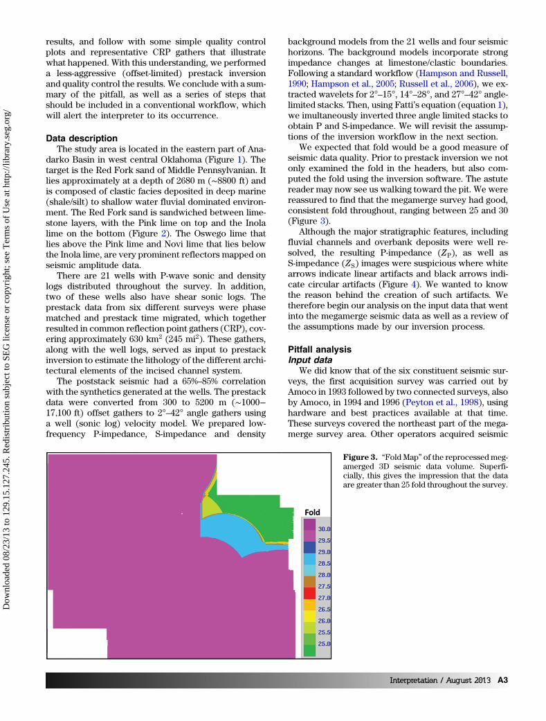
We expected that fold would be a good measure ofseismic data quality. Prior to prestack inversion we notonly examined the fold in the headers, but also com-puted the fold using the inversion software. The astutereader may now see us walking toward the pit. We werereassured to find that the megamerge survey had good,consistent fold throughout, ranging between 25 and 30(Figure 3).

Although the major stratigraphic features, includingfluvial channels and overbank deposits were well re-solved, the resulting P-impedance (ZP), as well asS-impedance (ZS) images were suspicious where whitearrows indicate linear artifacts and black arrows indi-cate circular artifacts (Figure 4). We wanted to knowthe reason behind the creation of such artifacts. Wetherefore begin our analysis on the input data that wentinto the megamerge seismic data as well as a review ofthe assumptions made by our inversion process.

Pitfall analysisInput data

We did know that of the six constituent seismic sur-veys, the first acquisition survey was carried out byAmoco in 1993 followed by two connected surveys, alsoby Amoco, in 1994 and 1996 (Peyton et al., 1998), usinghardware and best practices available at that time.These surveys covered the northeast part of the mega-merge survey area. Other operators acquired seismic

Figure 3. “Fold Map” of the reprocessed meg-amerged 3D seismic data volume. Superfi-cially, this gives the impression that the dataare greater than 25 fold throughout the survey.

Interpretation / August 2013 A3

Dow

nloa

ded

08/2

3/13

to 1

29.1

5.12

7.24

5. R

edis

trib

utio

n su

bjec

t to

SEG

lice

nse

or c

opyr

ight

; see

Ter

ms

of U

se a

t http

://lib

rary

.seg

.org

/

surveys imaging in the adjacent acreage from the years1999–2005 with relatively larger source-receiver offsets.Further analysis will reveal these larger source-receiveroffsets to be about 4600 m (15,000 ft). In 2006, the datafrom different companies were licensed to CGGVeritas.CCGVeritas acquired some additional data to fill inimportant gaps prior to merging all the componentsurveys into a single prestack dataset using modern(year 2008) statics solutions, noise attenuation, andseismic imaging technology.

Assumptions for prestack inversionWe use commercial software prestack seismic inver-

sion based on Fatti et al.’s (1994) approximation to theZoeppritz equations

RðθÞ ≈ ΔZP

2ZPð1þ tan2 θÞ − 8

�Zs

ZP

�2 ΔZs

2Zssin2 θ; (1)

where ZP ¼ average or background model P-imped-ance, ZS ¼ average or background model S-impedance,ΔZP and ΔZS ¼ the vertical change in P- and S-imped-ances, and θ ¼ the angle of incidence.

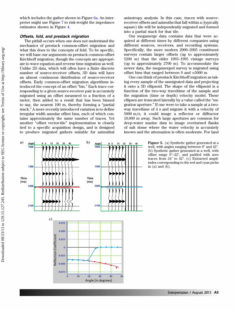
The modeled prestack response using equation 1 wastied to a well in the survey (Figure 5). The synthetic rep-resents an NMO-corrected gather such that the reflec-tors are aligned. Examining the reflector marked by thered line shows amplitudes becoming more negativewith increasing angle of incidence, θ. In conventionalAVO analysis, we would simply measure this changeand call it the amplitude “slope” or “gradient” whilethe value at θ ¼ 00 would be called the “intercept.”Many modern prestack inversion software implementa-tions use iterative modeling based on either simulatedannealing or genetic algorithms using equation 1 to fitthe data and thus estimate ZP and ZS.

The derivation of the gradient term, or alternativelyestimation of ZP and ZS, requires the reflectors to bealigned across the incident angle. Although it is wellunderstood that the inversion on misaligned prestackgathers produces incorrect results, users can easily en-counter a pitfall if they do not carefully examine thedata or have too much faith in their technology. Suchresidual moveout is best corrected by residual velocityanalysis, although trim statics may work within a rela-tively small analysis window. The red curve in Figure 5cshows the plot of amplitude variation with angle of thesynthetic modeled for 0°–45° corresponding to thepicked horizon in Figure 5a. In Figure 5b, we replacethe farther 25°–45° angles in the gather with zero am-plitude traces. The gradient corresponding to the ampli-tudes along the cyan pick in Figure 5b are displayed asthe cyan curve in Figure 5c. Obviously, this latter am-plitude variation with the angle will generate an inaccu-rate gradient and inaccurate estimate of ZP and ZS.

Modeled to measured data misfitTo better understand the problem, we examined a

suite of migrated CRP gathers at different locationsacross the megamerge survey (Figure 6). We notethat the reflector along the green Oswego pick hasstrong amplitudes aligned up to offsets of 4250 m(∼14;000 ft) at location A. At location C (Figure 6c),the alignment is good to about 4000 m (∼12;000 ft).At locations B and D (Figure 6b and 6d), this eventis aligned up to only 3050 m (∼10;000 ft). Beyond thispoint, the amplitudes are close to zero.

To validate our impedance inversion, we generatedthe synthetic data with the inversion products. Then, wesubtracted the synthetic from the original gathers andcreated a mean squared error volume. A horizon slicethrough this error volume along the top Oswego showsthat the highest error areas (appearing as red) are inthe northeast and east side of the megamerge survey(Figure 7). This includes the gathers shown in Figure 6band 6d. This area also corresponds to the suspicious ar-tifacts seen on the ZP and ZS slices shown in Figure 4.The best fit was in the northwest part of the survey,

Figure 4. Phantom horizon slices 80 ms below Oswegocutting the Red Fork incised channels through (a) the P-impedance volume, ZP (b) the S-impedance volume, ZS, com-puted from 2° to 42° input migrated gathers. For both of thefigures, white arrows indicate artifacts in the resulting image.Black dotted arrow indicates a circular artifact.

A4 Interpretation / August 2013

Dow

nloa

ded

08/2

3/13

to 1

29.1

5.12

7.24

5. R

edis

trib

utio

n su

bjec

t to

SEG

lice

nse

or c

opyr

ight

; see

Ter

ms

of U

se a

t http

://lib

rary

.seg

.org

/

which includes the gather shown in Figure 6a. An inter-preter might use Figure 7 to risk-weight the impedanceestimates shown in Figure 4.

Offsets, fold, and prestack migrationThe pitfall occurs when one does not understand the

mechanics of prestack common-offset migration andwhat this does to the concepts of fold. To be specific,we will base our arguments on prestack common-offsetKirchhoff migration, though the concepts are appropri-ate to wave equation and reverse time migration as well.Unlike 2D data, which will often have a finite discretenumber of source-receiver offsets, 3D data will havean almost continuous distribution of source-receiveroffsets. Early common-offset migration algorithms in-troduced the concept of an offset “bin.” Each trace cor-responding to a given source-receiver pair is accuratelymigrated using an offset measured to a fraction of ameter, then added to a result that has been binnedto say, the nearest 100 m, thereby forming a “partialstack.” Amore recently introduced variation is to defineirregular width annular offset bins, each of which con-tains approximately the same number of traces. Yetanother “offset vector-tile” implementation is closelytied to a specific acquisition design, and is designedto produce migrated gathers suitable for azimuthal

anisotropy analysis. In this case, traces with source-receiver offsets and azimuths that fall within a (typicallysquare) tile will be independently migrated and formedinto a partial stack for that tile.

Our megamerge data contains data that were ac-quired at different times by different companies usingdifferent sources, receivers, and recording systems.Specifically, the more modern 2000–2005 constituentsurveys contain larger offsets (up to approximately5200 m) than the older 1993–1995 vintage surveys(up to approximately 2700 m). To accommodate thenewer data, the megamerged survey is migrated usingoffset bins that ranged between 0 and ≈5000 m.

One can think of prestack Kirchhoff migration as tak-ing every sample of the unmigrated data and projectingit onto a 3D ellipsoid. The shape of the ellipsoid is afunction of the two-way traveltime of the sample andthe migration (time or depth) velocity model. Theseellipses are truncated laterally by a value called the “mi-gration aperture.” If one were to take a sample at a two-way traveltime of 4 s and migrate it with a velocity of5000 m∕s, it could image a reflector or diffractor10,000 m away. Such large apertures are common fordeep-water marine data to image overturned flanksof salt dome where the water velocity is accuratelyknown and the attenuation is often moderate. For land

Figure 5. (a) Synthetic gather generated at awell, with angles ranging between 0° and 42°.(b) Synthetic gather generated at a well, withoffset range 0°–22°, and padded with zerotraces from 24° to 42°. (c) Extracted ampli-tudes corresponding to the red and cyan picksin (a) and (b).

Interpretation / August 2013 A5

Dow

nloa

ded

08/2

3/13

to 1

29.1

5.12

7.24

5. R

edis

trib

utio

n su

bjec

t to

SEG

lice

nse

or c

opyr

ight

; see

Ter

ms

of U

se a

t http

://lib

rary

.seg

.org

/

data, extremely large migration apertures are usuallyavoided, not only for cost, but because of problemsin accurately defining the attenuation and velocity mod-els. This restricted approach is more common in rela-tively flat-lying areas such as those imaged by thissurvey. We do not know the migration aperture usedfor this megamerge, but a reasonable guess would besomewhat less than 5000 m. Using this number, we thenfound that the far offset data acquired in the northwestpart of the survey would be migrated or “swung” 5000 minto areas covered by the short-offset vintage surveys.Interpreters commonly encounter such “migrationswings” on migrated stacked data volumes at the edgesof their surveys or underneath obstacles such as townsand lakes. Thus, the “data” at the farther offsets shownin Figure 6b, Figure 6c, and 6d are not from the over-lying survey, but rather migrated noise from an adja-cent, more modern survey. Far offsets that have littleto no data in them will appear to have been “padded”with near-zero value traces. A small amount of migra-tion swing will cause a trace to have data in it, prevent-ing it from being flagged as “dead.” Thus, the fold maprepresents the 30 offset bins of the migrated data, notthe fold of the original unmigrated surveys (Figure 3).The lower fold seen in the northeast corner of the meg-amerge clearly shows the circular limits corresponding

to the migration aperture from the corners of neighbor-ing longer offset constituent surveys.

Validation of our hypothesisThe original input surveys and their acquisition

and processing information were not available; the onlyseismic data available were the gathers of the migratedmegamerged survey. To identify the usable offsetranges for the data, we picked the peak, which corre-sponds to the Oswego lime horizon on the full stackvolume, and generated horizon slices through a suiteof offset-limited stacks. Because of the AVO effects,we do not expect these slices to show a consistentpolarity. Figure 8a–8c shows a nearly constant bluevalue corresponding to a positive peak for offset-limitedstacks of 0–1520 m (∼0−5000 ft), 1520–2450 m(∼5000−8000 ft), and 2450–3350 m (8000–11,000 ft).The change from blue (positive) to green (less positive)values in Figure 8c is an acceptable AVO effect. How-ever, as we examine the horizon slice through the off-set-limited stack at 3350–4250 m (∼11000−14000 ft), wenote lower (positive and negative) amplitudes and lesscontinuous anomalies in the northeast part of the meg-amerge survey. Finally, the horizon slice through theoffset-limited stack of 4250–5200 m (∼14000−17100 ft)shows zero or near-zero amplitude (white area) in the

Figure 6. Representative gathers and basemap indicating their locations. Note that loca-tions (a and d) have moderate amplitudeswhereas (b and c) have low amplitudes atthe farther offsets. The small residual ampli-tudes beyond these ranges are due to migra-tion swings from the longer offset surveys.

A6 Interpretation / August 2013

Dow

nloa

ded

08/2

3/13

to 1

29.1

5.12

7.24

5. R

edis

trib

utio

n su

bjec

t to

SEG

lice

nse

or c

opyr

ight

; see

Ter

ms

of U

se a

t http

://lib

rary

.seg

.org

/

northeast corner of the megamerge corresponding tothe shorter offset acquisition of the 1993–1995 Amocosurveys (Peyton et al., 1998). Note the circular migra-

tion “impulse responses” seen in this part of the surveywhere some of the more modern, longer offset infilldata have been migrated into the shorter offset data.

The solution — Inversion using shorter offsetsGiven the result of this analysis, it is inappropriate to

use the images shown in Figure 4 for the entire survey.To obtain a uniform quality inversion for the entire sur-vey, we limit the offsets of our inversion to the range0–2750 m (0–9000 ft). At the target Red Fork horizon(below the Oswego), these offsets correspond to anangle range of 2°–22°. Such a near angle limitation pre-cludes inversion for density (Aki and Richards, 1980);however, we can still invert for ZP and ZS using equa-tion 1, though with lower confidence (Plessix and Bork,2000) than we had originally anticipated using largerangles. We use the same low-frequency backgroundmodel as for Figure 4, but this time extract three wave-lets for inversion at 2°–9°, 9°–15°, and 14°–22°. Theprestack simultaneous inversion shown in Figure 9has none of the artifacts seen in Figure 4. The back-ground amplitude varies relatively smoothly, showingthe incised channels of variable fill more clearly.

Figure 8. Horizon slices along the Oswegosurface through offset-limited stacked ampli-tude volumes: (a) 0–1520 m (∼0–5000 ft),(b) 1520–2450 m (∼5000–8000 ft), (c) 2450–3350 m (∼8000–11;000 ft), (d) 3350–4250 m(∼11;000–14;000 ft), and (e) 4250–5200 m(∼14;000–17;100 ft). The Oswego Lime was in-terpreted as a strong peak in the stacked seis-mic volume. Amplitude changes in (c) may bevalid AVO effects. Often, inaccurate velocities(including anisotropic effects) result in mis-aligned gathers giving rise to zero crossingsand troughs at far offsets. However, notehow the amplitude approaches zero in thetop right corner of the megamerged surveyin (d and e) indicating that these large offsetswere never recorded in these areas. Whitepolygons in (c) indicate amplitude anomaliesthat will be used in subsequent quality control.White arrows indicate the major highways.

Figure 7. Mean-squared error map showing the differencebetween the measured and modeled seismic gathers for the2°–42° inversion.

Interpretation / August 2013 A7

Dow

nloa

ded

08/2

3/13

to 1

29.1

5.12

7.24

5. R

edis

trib

utio

n su

bjec

t to

SEG

lice

nse

or c

opyr

ight

; see

Ter

ms

of U

se a

t http

://lib

rary

.seg

.org

/

Readers interested in the geologic analysis of these in-cisions should refer to Del Moro (2012).

Following our earlier quality control steps, we com-pute the squared difference between the modeled andmeasured data for 2°–22°, and display a time slice alongthe Oswego top through the error volume in Figure 10using the same color bar and scale as in the 2°–42° in-version shown in Figure 7. Although we have restrictedthe input seismic to 2°–22° to avoid the error, we stillsee some areas of misfit, such as about the north-north-west–south-southeast trending highway imaged usingthe 1993 acquisition. Interestingly, the east–west trend-ing highway to the south is much more heavily traveledbut was acquired by a more recent survey. The pinkpolygon in Figures 9 and 10 appears to be associatedwith subsurface geology though not with the channels,or to the present day river flowing in northwest–south-east direction. This suggests that the offset restrictionof 0–4250 m is good for most of the areas, but the actualoffset range was even smaller than 4250 m in some

areas. A more careful inversion would be adaptive fordifferent angle ranges in different parts of the mega-merge survey.

ConclusionsLegacy seismic data acquired by different companies

using different acquisition parameters over adjacentacreage can be merged into a larger survey that canbe subsequently imaged using a larger migration aper-ture, thereby improving lateral resolution. “Fold” onmigrated data traces should be suspect, and dependson whether the processor retained the fold of the inputsurveys through the complete data equalization and re-processing flow, or carefully computed the illuminationat each subsurface point using a more sophisticated im-aging technique. Fold count after migration can be mis-leading as a proxy to measure signal strength.

If a given input survey is acquired using shorteroffsets, Kirchhoff and other common-offset migrationalgorithms will generate numerical noise on the paddedfar offset empty traces. It can also generate steeply dip-ping signals. In general, such far offsets should notbe used in prestack inversion. Because of migration“swings,” these unilluminated offsets will rarely, if ever,be zero, making automatic detection of dead traces dif-ficult. This leads the unsuspecting interpreter and inver-sion algorithm to believe that such traces containmeasured data. Prestack inversion will attempt to findimpedances and densities that will fit all the migrateddata, including unilluminated offsets that are close tozero, giving erroneous results.

To avoid such pitfalls, we first suggest that inter-preters generate root-mean-square error maps of themodeled-to-measured data misfit for any inversionproduct. Such maps can be used in subsequent risk

Figure 9. Phantom horizon slices 80 ms below the Oswegothrough (a) the P-impedance volume, ZP, (b) the S-impedancevolume, ZS, computed from 2°–22° input migrated gathers.Pink polygons correspond to an area of high error shownin Figure 10.

Figure 10. Mean squared error map showing the differencebetween the measured and modeled seismic gathers for the2°–22° inversion. To compare with Figure 6, the squared errorwas normalized with respect to the number of traces in eachgather. White arrow corresponds to those drawn about ampli-tude anomalies shown in Figure 8c. Pink polygons encircle anarea of high error that is posted on Figure 9.

A8 Interpretation / August 2013

Dow

nloa

ded

08/2

3/13

to 1

29.1

5.12

7.24

5. R

edis

trib

utio

n su

bjec

t to

SEG

lice

nse

or c

opyr

ight

; see

Ter

ms

of U

se a

t http

://lib

rary

.seg

.org

/

analysis. It is valuable to see the prestack gathers of dif-ferent parts of the megamerge survey, but this could bereally time-consuming. So, for megamerge surveyswhere the offsets of the constituent input survey vol-umes are unknown, the interpreter should generatetime or horizon slices through amplitude volumes foreach of the offsets. Subsequent inversions should beoffset- (and implicitly, angle-) limited to include onlythose offsets with physically reasonable amplitudes.

AcknowledgmentsWe thank CGGVERITAS for providing the mega-

merge seismic survey and Chesapeake Energy for thewell data used in this project. Special thanks to AlfredoFernandez of OU, for his valuable suggestions andthanks to Sara Chilson for grammatical corrections.Funding for the research was provided by the industrysponsors of the Attribute-Assisted Seismic Processingand Interpretation consortium. Finally, we thankSchlumberger for Petrel and Hampson-Russell forStrata software licenses provided to The Universityof Oklahoma for research and education.

ReferencesAki, K., and P. G. Richards, 1980, Quantitative seismology:

Theory and methods: Freeman and Co.Barber, R., and K. J. Marfurt, 2010, Challenges in mapping

seismically invisible Red Fork channels, AnadarkoBasin, Oklahoma: The Shale Shaker, 61, 147–163.

Clement, W., 1991, East Clinton Field-U.S.A. AnadarkoBasin, Oklahoma: AAPG Special Volumes, TR: Strati-graphic Traps II, 207–267.

Del Moro, Y. P., 2012, An integrated seismic geologic andpetro-physical approach to characterize the Red Forkincised valley fill system in the Anadarko basin:Oklahoma: M.S. thesis, The University of Oklahoma.

Del Moro, Y. P., A. Fernandez-Abad, and K. J. Marfurt,2013, Why should we pay for a merged survey thatcontains the data we already have? An OklahomaRed Fork example: The Shale Shaker, 63, 336–357.

Fatti, J. L., G. C. Smith, P. J. Vail, P. J. Strauss, and P. R.Levitt, 1994, Detection of gas in sandstone reservoirsusing AVO analysis: A 3-D seismic case history using theGeostack technique: Geophysics, 59, 1362–1376, doi: 10.1190/1.1443695.

Hampson, D., and B. H. Russell, 1990, AVO inversion:Theory and practice: 60th Annual International Meeting,SEG, Expanded Abstracts, 1456–1458.

Hampson, D. P., B. H. Russell, and B. Bankhead, 2005,Simultaneous inversion of pre-stack seismic data:75th Annual International Meeting, SEG, ExpandedAbstracts, 1633–1637.

Northcutt, R. A., and J. A. Campbell, 1988, Geologicprovinces of Oklahoma, OklahomaGeological Survey. ac-cessed 4 February 2013; http://www.faqs.org/sec-filings/111201/North-Texas-Energy-Inc_S-1/ex99-1.htm#b.

Peyton, L., R. Bottjer, and G. Partyka, 1998, Interpretationof incised valleys using new 3D seismic techniques: Acase history using spectral decomposition and coher-ency: The Leading Edge, 17, 1294–1298, doi: 10.1190/1.1438127.

Plessix, R. E., and J. Bork, 2000, Quantitative estimate ofVTI parameters from AVA responses: Geophysical Pro-specting, 48, 87–108, doi: 10.1046/j.1365-2478.2000.00175.x.

Russell, B., D. Hampson, and B. Bankhead, 2006, An inver-sion primer: CSEG Recorder, Special issue, 96–103.

Biographies and photos of the authors are not available.

Interpretation / August 2013 A9

Dow

nloa

ded

08/2

3/13

to 1

29.1

5.12

7.24

5. R

edis

trib

utio

n su

bjec

t to

SEG

lice

nse

or c

opyr

ight

; see

Ter

ms

of U

se a

t http

://lib

rary

.seg

.org

/