university of oklahoma prestack and poststack …
TRANSCRIPT
UNIVERSITY OF OKLAHOMA
GRADUATE COLLEGE
PRESTACK AND POSTSTACK ATTRIBUTE ANALYSIS OF THE JEJU BASIN,
KOREA
A THESIS
SUBMITTED TO THE GRADUATE FACULTY
in partial fulfillment of the requirements for the
Degree of
MASTER OF SCIENCE
By
OLANREWAJU AYODAPO ABOABA
Norman, Oklahoma
2015
PRESTACK AND POSTSTACK ATTRIBUTE ANALYSIS OF THE JEJU BASIN,
KOREA
A THESIS APPROVED FOR THE
CONOCOPHILLIPS SCHOOL OF GEOLOGY AND GEOPHYSICS
BY
______________________________
Dr. Kurt Marfurt, Chair
______________________________
Dr. John Pigott
______________________________
Dr. Jamie Rich

© Copyright by OLANREWAJU AYODAPO ABOABA 2015
All Rights Reserved.

All things are possible to those that believe.
iv
ACKNOWLEDGEMENTS
I am deeply grateful to Dr. Kurt Marfurt for his patience, guidance and believing
in me and pushing beyond my limits, all through the program and to my committee
members Dr. Jamie Rich and Dr. John Pigott for their useful contributions and
constructive criticisms. I also appreciate and miss the Late Dr. Tim Kwiatkowski for his
persistence, perseverance and commitment to help his students succeed.
I thank the Korea Institute of Geoscience and Mineral Resources (KIGAM) for
providing funding and data for research.
I thank Donna Mullins and Rebecca Fay for assisting with paper work,
Nancy Leonard, Devon Harr, Jocelyn Cook, Theresa Hackney for all their administrative
assistance and support at the ConocoPhillips School of Geology and Geophysics.
I would like to thank Ben Dowdell, Dalton Hawkins, Bo Zhang, Shiguang Guo
and Yuji Kim for their help with processing the seismic data. Thang Ha for helping with
the bug fixes on the AASPI software while running the attributes and processing. I am
truly appreciative of Toan Dao, Sumit Verma, Atish Roy, Brad Wallet, Tao Zhao, Fangyu
Li, Tengfei Lin, and all members of the AASPI consortium for their valuable suggestions
and contributions.
I thank the sponsors of the AASPI consortium. I give special thanks to Sue and
Barry of the Landmark Promax support desk.
I am also grateful to Sue Palmer who made me a beautiful diamond quilt as a
parting gift, Joyce Stiehler and Shanika Wilson of the Oklahoma Geological Survey.

v
I appreciate all my loving friends both within and without the state of Oklahoma
and the experiences we have shared, that have contributed in no small way to the success
of this program. You have all made my stay in Norman eventful and memorable.
I am also indebted to my family for their constant support, prayers and the values
of hard work and contentment they have instilled in me. This has helped me forge ahead
through thick and thin.
Finally, I am grateful to the Greatest Optimal Divinity my help in ages past and
my hope for years to come.

vi
TABLE OF CONTENTS
ACKNOWLEDGEMENTS ............................................................................................ iv
LIST OF TABLES ......................................................................................................... vii
LIST OF FIGURES ....................................................................................................... viii
ABSTRACT .................................................................................................................. xiii
CHAPTER 1: INTRODUCTION ..................................................................................... 1
CHAPTER 2: GEOLOGIC OVERVIEW ........................................................................ 4
CHAPTER 3: METHODOLOGY .................................................................................. 10
DATA AVAILABLE ............................................................................................... 10
SEISMIC PROCESSING ......................................................................................... 16
CHAPTER 4: DATA ANALYSIS AND INTERPRETATION .................................... 38
STRUCTURE OF MEGASEQUENCE BOUNDARIES AND SEAFLOOR ......... 38
STRATIGRAPHY OF MEGASEQUENCES .......................................................... 55
AMPLITUDE ANALYSIS OF OFFSET LIMITED STACKS. .............................. 64
IMPLICATIONS FOR HYDROCARBON PROSPECTIVITY .............................. 71
CHAPTER 5: CONCLUSIONS ..................................................................................... 73
REFERENCES ............................................................................................................... 76

vii
LIST OF TABLES
Table 1.0: Summary of acquisition parameters. ............................................................. 12
viii
LIST OF FIGURES
Figure 2.1: Structural and tectonic elements of the East China Sea. (Modified after (Zhou
et al., 1989; Yang 1992; Lee et al., 2006). HPJR = Hupijiao Rise, HJR= Haijao rise;
GYR= Gunyan Rise; YSR= Yusan rise; JB = Jeju Basin; SB = Socotra Basin; .............. 7
Figure 2.2: Summary of the evolutionary stages of the East China Sea Shelf Basin (after
Lee et. al., 2006). I will map MB1-MB4 in this 3D survey. MB = Megasequence
boundaries. ........................................................................................................................ 8
Figure 2.3: Summary of sedimentary environments, potential reservoirs and source rocks
during the evolution of the northern East China Sea shelf basin. (Lee et al., 2006). ....... 9
Figure 3.1: R/V Tamhae II vessel used for seismic acquisition (Courtesy of KIGAM). 13
Figure 3.2: Location map of survey area relative to Jeju Island. Red rectangle combines
2012 and 2013 acquisition lines. Orange rectangle is phase 3 survey acquired in 2014
perpendicular to the red rectangle. Black circle is Dragon-1 well location. .................. 14
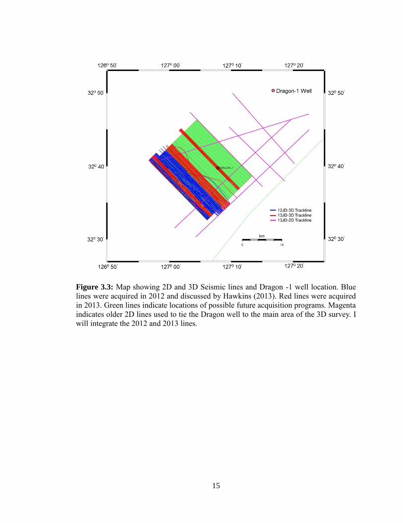
Figure 3.3: Map showing 2D and 3D Seismic lines and Dragon -1 well location. Blue
lines were acquired in 2012 and discussed by Hawkins (2013). Red lines were acquired
in 2013. Green lines indicate locations of possible future acquisition programs. Magenta
indicates older 2D lines used to tie the Dragon well to the main area of the 3D survey. I
will integrate the 2012 and 2013 lines. ........................................................................... 15
Figure 3.4: Seismic Processing Workflow. The processes in yellow were conducted using
Promax. Those in white were conducted using OU software. ....................................... 24
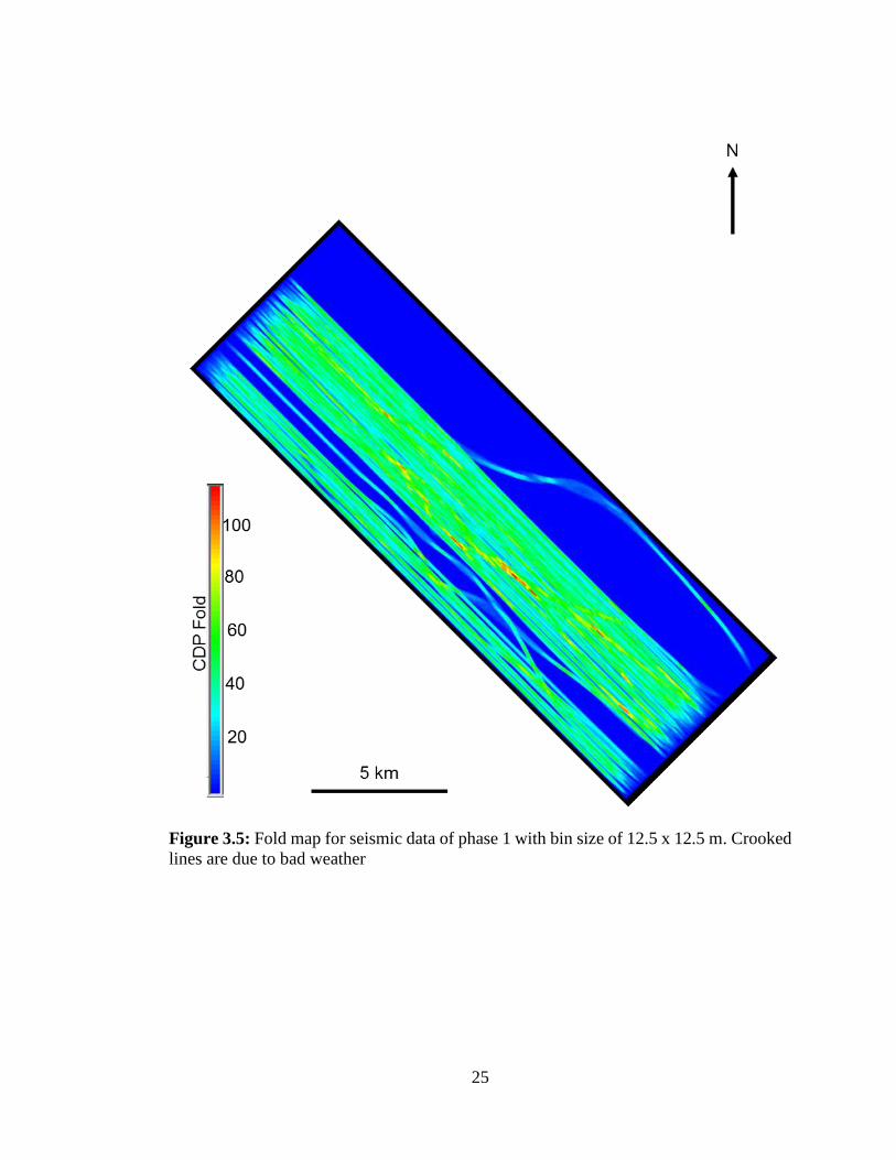
Figure 3.5: Fold map for seismic data of phase 1 with bin size of 12.5 x 12.5 m. Crooked
lines are due to bad weather ........................................................................................... 25
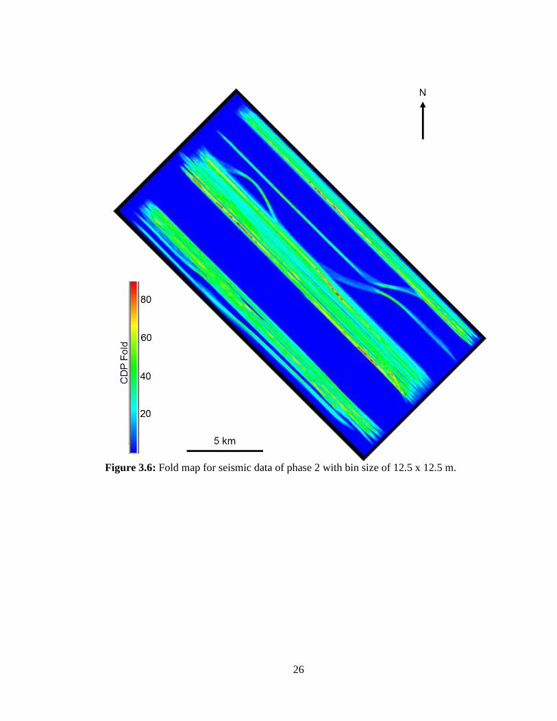
Figure 3.6: Fold map for seismic data of phase 2 with bin size of 12.5 x 12.5 m. ......... 26
ix
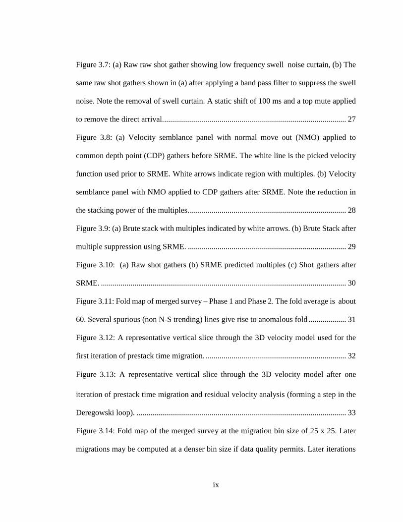
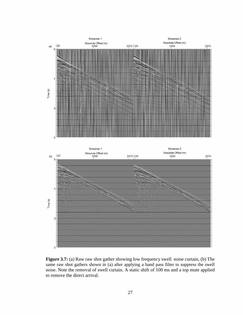
Figure 3.7: (a) Raw raw shot gather showing low frequency swell noise curtain, (b) The
same raw shot gathers shown in (a) after applying a band pass filter to suppress the swell
noise. Note the removal of swell curtain. A static shift of 100 ms and a top mute applied
to remove the direct arrival. ............................................................................................ 27
Figure 3.8: (a) Velocity semblance panel with normal move out (NMO) applied to
common depth point (CDP) gathers before SRME. The white line is the picked velocity
function used prior to SRME. White arrows indicate region with multiples. (b) Velocity
semblance panel with NMO applied to CDP gathers after SRME. Note the reduction in
the stacking power of the multiples. ............................................................................... 28
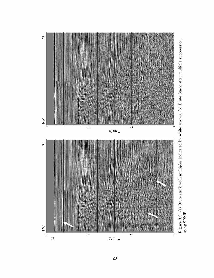
Figure 3.9: (a) Brute stack with multiples indicated by white arrows. (b) Brute Stack after
multiple suppression using SRME. ................................................................................ 29
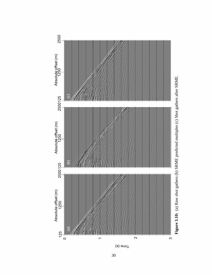
Figure 3.10: (a) Raw shot gathers (b) SRME predicted multiples (c) Shot gathers after
SRME. ............................................................................................................................ 30
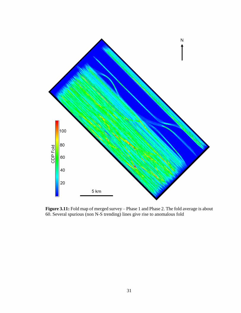
Figure 3.11: Fold map of merged survey – Phase 1 and Phase 2. The fold average is about
60. Several spurious (non N-S trending) lines give rise to anomalous fold ................... 31
Figure 3.12: A representative vertical slice through the 3D velocity model used for the
first iteration of prestack time migration. ....................................................................... 32
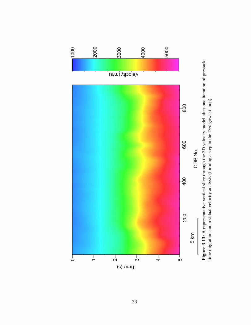
Figure 3.13: A representative vertical slice through the 3D velocity model after one
iteration of prestack time migration and residual velocity analysis (forming a step in the
Deregowski loop). .......................................................................................................... 33
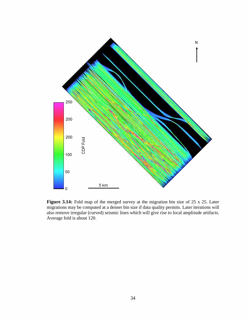
Figure 3.14: Fold map of the merged survey at the migration bin size of 25 x 25. Later
migrations may be computed at a denser bin size if data quality permits. Later iterations

x
will also remove irregular (curved) seismic lines which will give rise to local amplitude
artifacts. Average fold is about 120. ............................................................................... 34
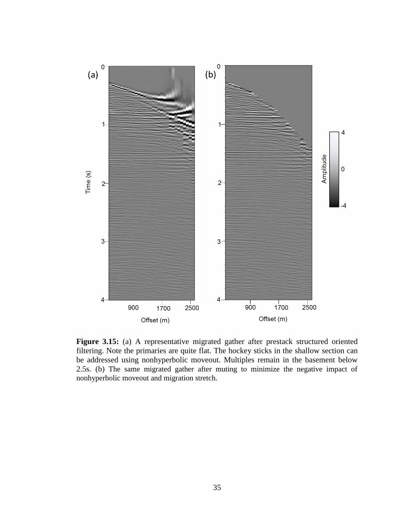
Figure 3.15: (a) A representative migrated gather after prestack structured oriented
filtering. Note the primaries are quite flat. The hockey sticks in the shallow section can
be addressed using nonhyperbolic moveout. Multiples remain in the basement below
2.5s. (b) The same migrated gather after muting to minimize the negative impact of
nonhyperbolic moveout and migration stretch. .............................................................. 35
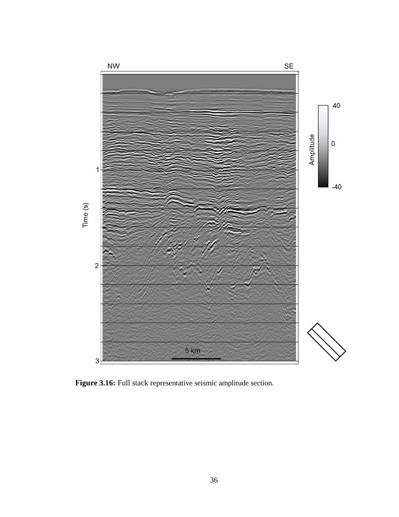
Figure 3.16: Full stack representative seismic amplitude section. ................................. 36
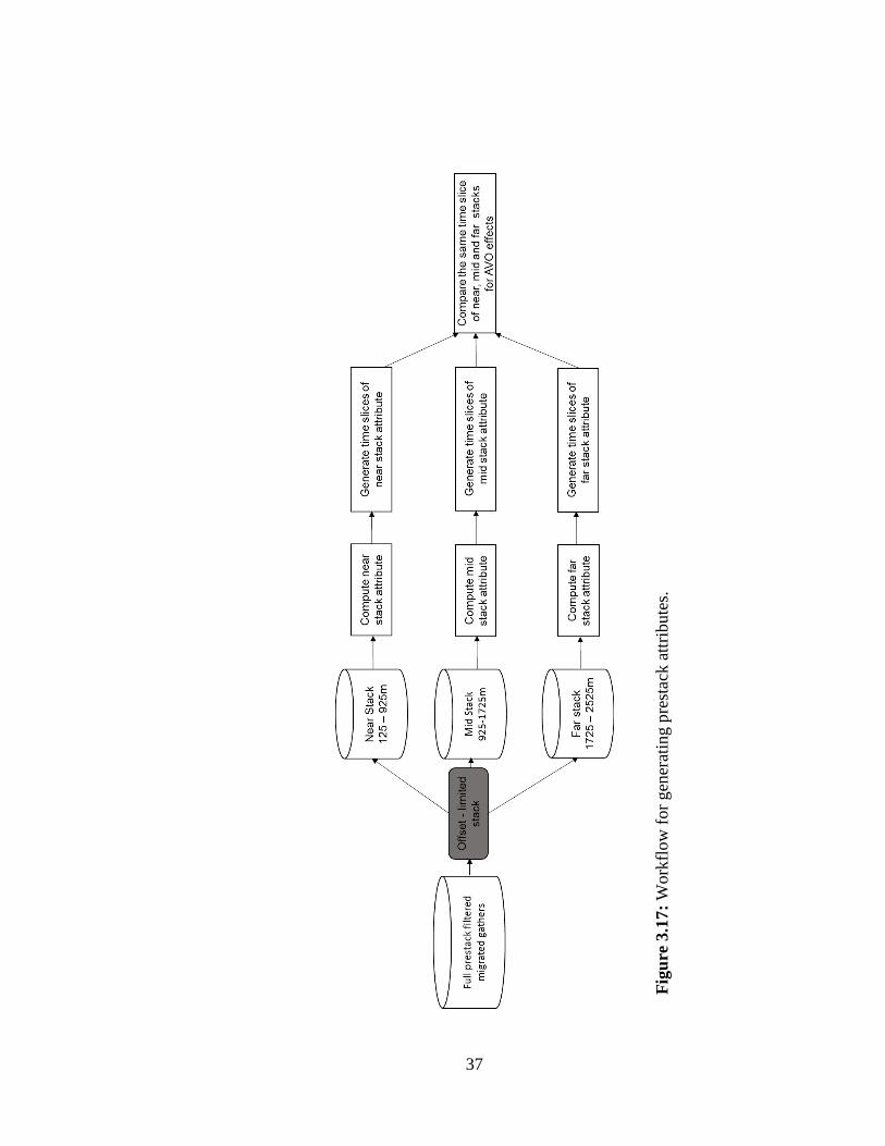
Figure 3.17: Workflow for generating prestack attributes. ............................................ 37
Figure 4.1: Coherent energy section showing anomalous high coherence indicated by
white arrows. These anomalies are not geological but due to cable feathering. Blue arrows
indicate high amplitude anomalies that are geologically reasonable. ............................ 42
Figure 4.2: Sobel filter similarity section. Red arrows indicate faults. .......................... 43
Figure 4.3: Seismic amplitude co-rendered with most positive curvature in red and most
negative curvature in blue. ............................................................................................. 44
Figure 4.4: Interpreted seismic section showing southeast dipping faults in yellow and
antithetic faults in light blue. MB = Megasequence boundary, MS = Megasequence. .. 45
Figure 4.5: Time structure map of MB1. ........................................................................ 46
Figure 4.6: Time structure map of MB2. ........................................................................ 47
Figure 4.7: Time structure map of MB3. ....................................................................... 48
Figure 4.8: Horizon slice along MB3 of (a) dip magnitude and (b) dip azimuth volumes.
Red and white arrows indicate faults. ............................................................................. 49
xi
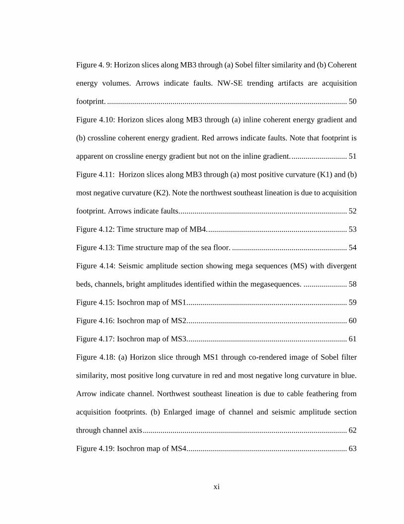
Figure 4. 9: Horizon slices along MB3 through (a) Sobel filter similarity and (b) Coherent
energy volumes. Arrows indicate faults. NW-SE trending artifacts are acquisition
footprint. ......................................................................................................................... 50
Figure 4.10: Horizon slices along MB3 through (a) inline coherent energy gradient and
(b) crossline coherent energy gradient. Red arrows indicate faults. Note that footprint is
apparent on crossline energy gradient but not on the inline gradient. ............................ 51
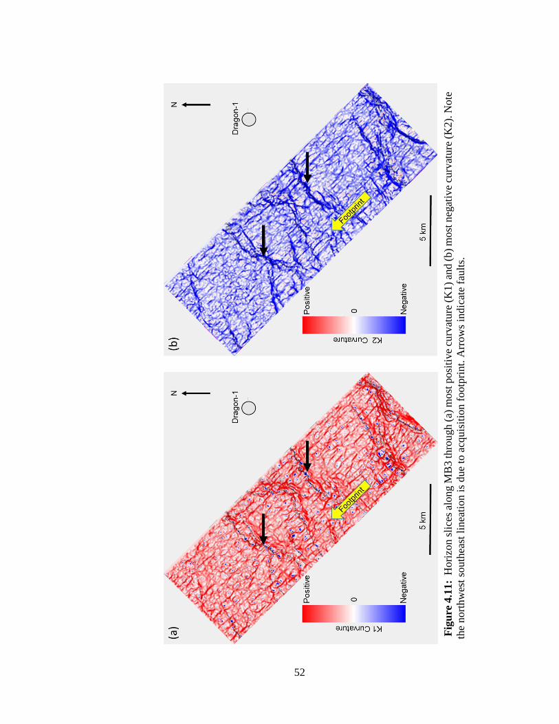
Figure 4.11: Horizon slices along MB3 through (a) most positive curvature (K1) and (b)
most negative curvature (K2). Note the northwest southeast lineation is due to acquisition
footprint. Arrows indicate faults. .................................................................................... 52
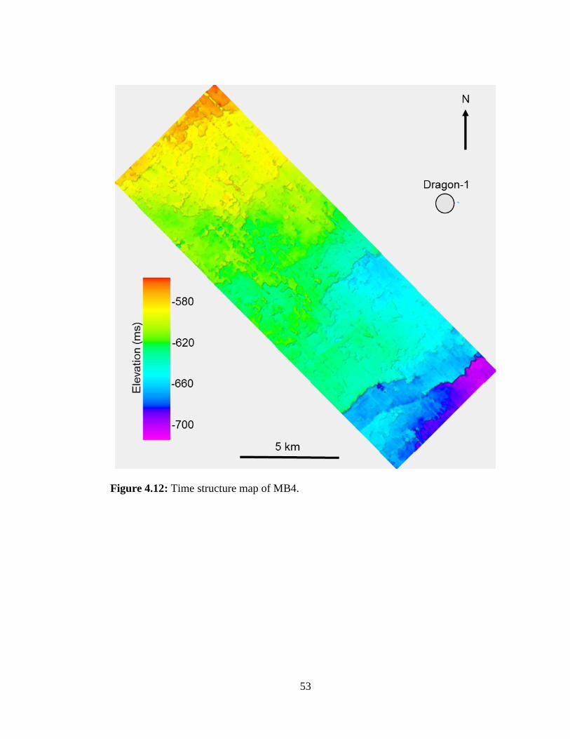
Figure 4.12: Time structure map of MB4. ...................................................................... 53
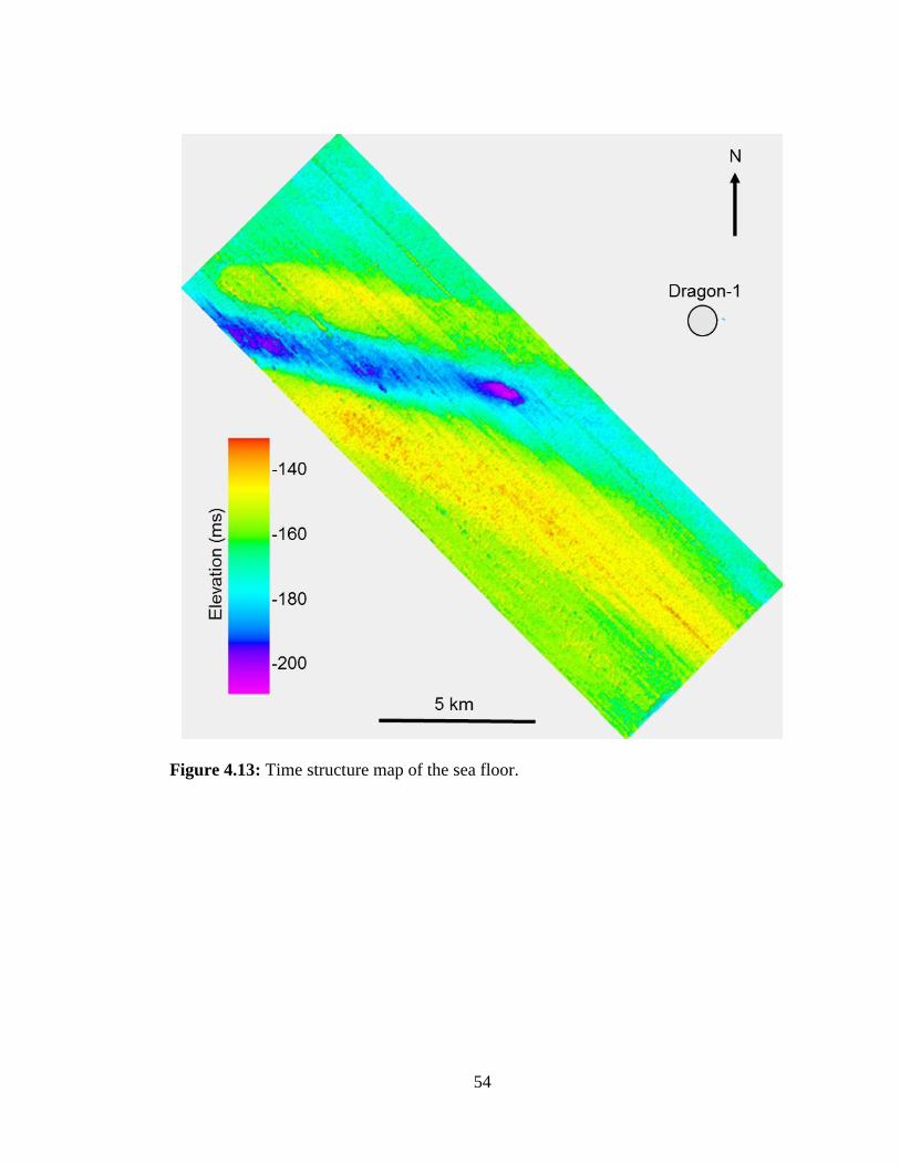
Figure 4.13: Time structure map of the sea floor. .......................................................... 54
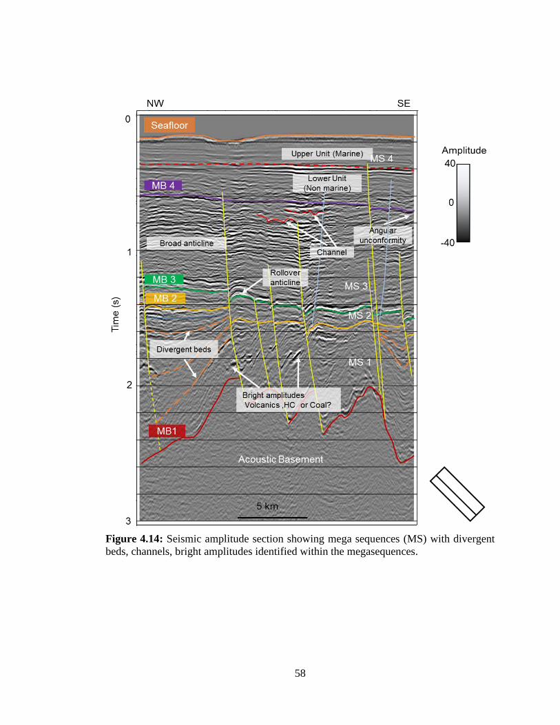
Figure 4.14: Seismic amplitude section showing mega sequences (MS) with divergent
beds, channels, bright amplitudes identified within the megasequences. ...................... 58
Figure 4.15: Isochron map of MS1. ................................................................................ 59
Figure 4.16: Isochron map of MS2. ................................................................................ 60
Figure 4.17: Isochron map of MS3. ................................................................................ 61
Figure 4.18: (a) Horizon slice through MS1 through co-rendered image of Sobel filter
similarity, most positive long curvature in red and most negative long curvature in blue.
Arrow indicate channel. Northwest southeast lineation is due to cable feathering from
acquisition footprints. (b) Enlarged image of channel and seismic amplitude section
through channel axis ....................................................................................................... 62
Figure 4.19: Isochron map of MS4 ................................................................................. 63
xii
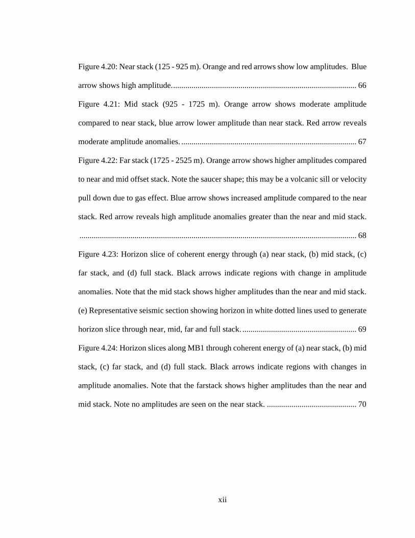
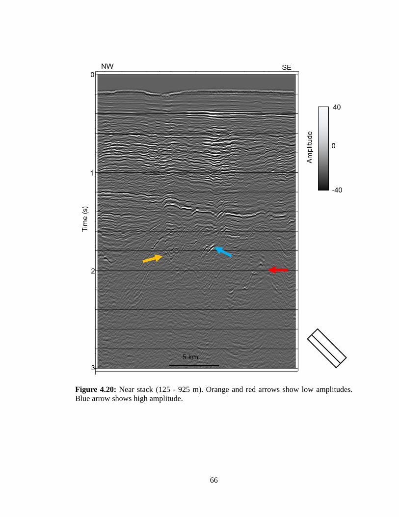
Figure 4.20: Near stack (125 - 925 m). Orange and red arrows show low amplitudes. Blue
arrow shows high amplitude. .......................................................................................... 66
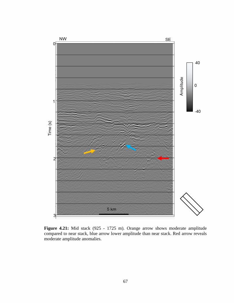
Figure 4.21: Mid stack (925 - 1725 m). Orange arrow shows moderate amplitude
compared to near stack, blue arrow lower amplitude than near stack. Red arrow reveals
moderate amplitude anomalies. ...................................................................................... 67
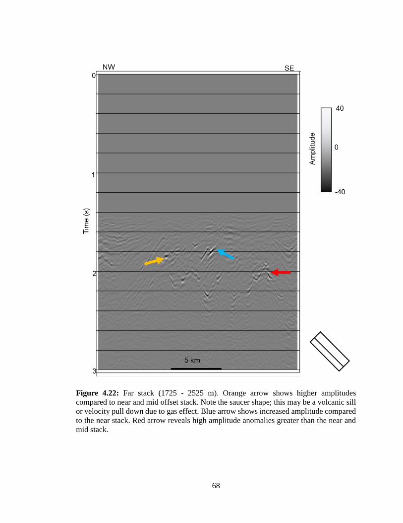
Figure 4.22: Far stack (1725 - 2525 m). Orange arrow shows higher amplitudes compared
to near and mid offset stack. Note the saucer shape; this may be a volcanic sill or velocity
pull down due to gas effect. Blue arrow shows increased amplitude compared to the near
stack. Red arrow reveals high amplitude anomalies greater than the near and mid stack.
........................................................................................................................................ 68
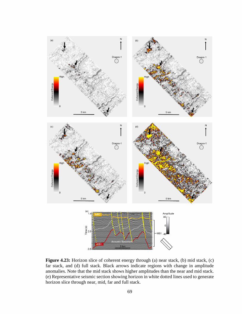
Figure 4.23: Horizon slice of coherent energy through (a) near stack, (b) mid stack, (c)
far stack, and (d) full stack. Black arrows indicate regions with change in amplitude
anomalies. Note that the mid stack shows higher amplitudes than the near and mid stack.
(e) Representative seismic section showing horizon in white dotted lines used to generate
horizon slice through near, mid, far and full stack. ........................................................ 69
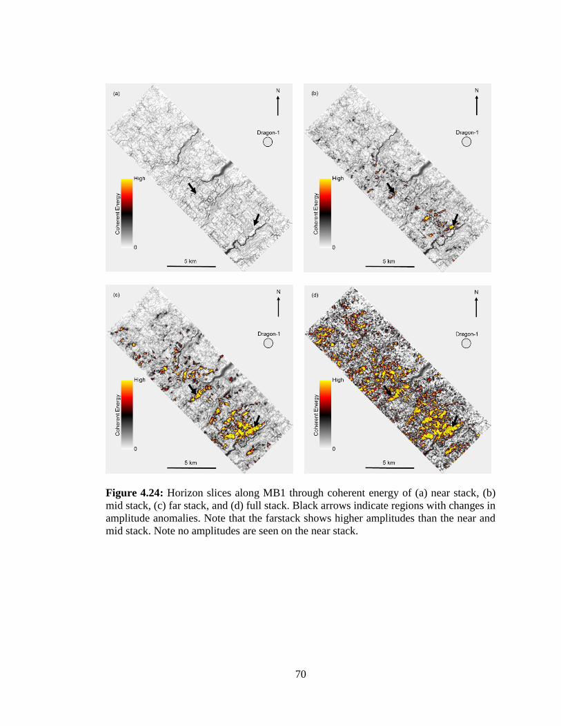
Figure 4.24: Horizon slices along MB1 through coherent energy of (a) near stack, (b) mid
stack, (c) far stack, and (d) full stack. Black arrows indicate regions with changes in
amplitude anomalies. Note that the farstack shows higher amplitudes than the near and
mid stack. Note no amplitudes are seen on the near stack. ............................................ 70
xiii
ABSTRACT
The Korean Institute for Geosciences and Mineral Resources acquired 3D marine
seismic in two phases during 2012 and 2013 to understand the structural and stratigraphic
controls for possible hydrocarbon accumulation.
This thesis documents the processing of the phase 2 survey as well as the
migration and interpretation of the merged phase 1 and phase 2 surveys. Two-dimensional
surface related multiple elimination suppressed the multiples; true amplitude recovery
balanced the amplitude and deconvolution improved temporal resolution. The merged
volume passed through velocity analysis, residual velocity analysis, Kirchhoff prestack
time migration, prestack structured oriented filtering and final stacked volumes of near,
mid, far and full offsets. Poststack attributes revealed presence of strong acquisition
footprint because of cable feathering as evident from curvature, dip magnitude and
coherent energy attribute volumes.
The migrated survey illuminates structural features including roll over anticlines,
half grabens, and basement-induced faults cutting into shallow beds all of which form
potential hydrocarbon traps. Parallel beddings, erosional truncations, angular
unconformities, fluvial features are stratigraphic features that populate the shallower
section, while divergent beds are seen at the deeper section. Bright amplitudes terminated
against faults blocks. Four mega sequences boundaries and the sea floor were identified,
with their corresponding time maps generated. Isochron maps of mega sequences
revealed that the maximum thickness within each of the megasequence increased from
proximal to distal from the oldest to the youngest sequence. The time maps and attribute

xiv
volumes of horizon slices showed variability in the faulting architecture and
compartmentalization spatially and in time, and highlighted channelization.
Horizon slices of coherent energy of near, mid and far stacks through MS1
showed variability in amplitudes with higher amplitudes in the mid stack than the near
and far. However, the far stack showed higher amplitudes at the base of the sequence. In
addition, the seismic section of the far stack showed a higher illumination of the acoustic
basement than the near and mid stack. Without well control, this variation in amplitudes
could be due to hydrocarbon, volcanic emplacement, or coal indicating significant risk,
but also potential promise to subsequent hydrocarbon exploration.
1
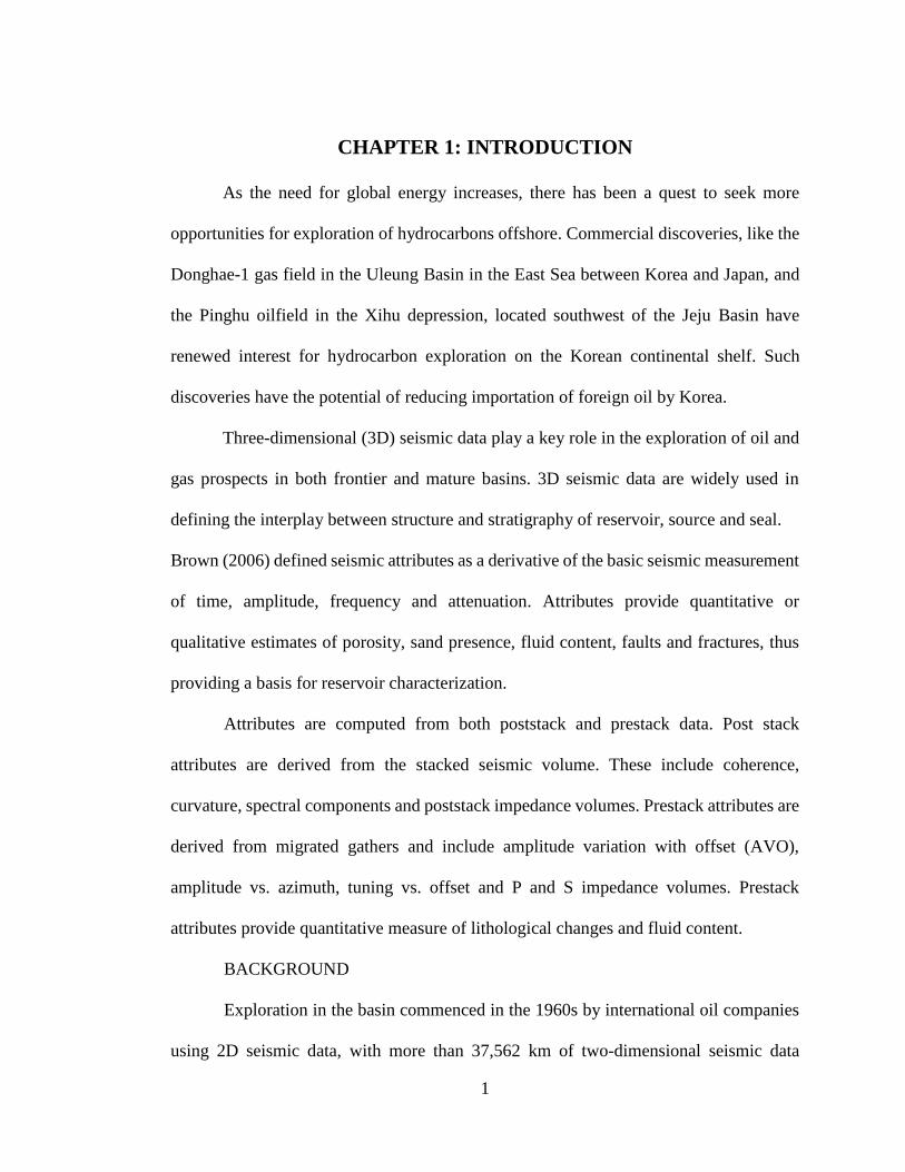
CHAPTER 1: INTRODUCTION
As the need for global energy increases, there has been a quest to seek more
opportunities for exploration of hydrocarbons offshore. Commercial discoveries, like the
Donghae-1 gas field in the Uleung Basin in the East Sea between Korea and Japan, and
the Pinghu oilfield in the Xihu depression, located southwest of the Jeju Basin have
renewed interest for hydrocarbon exploration on the Korean continental shelf. Such
discoveries have the potential of reducing importation of foreign oil by Korea.
Three-dimensional (3D) seismic data play a key role in the exploration of oil and
gas prospects in both frontier and mature basins. 3D seismic data are widely used in
defining the interplay between structure and stratigraphy of reservoir, source and seal.
Brown (2006) defined seismic attributes as a derivative of the basic seismic measurement
of time, amplitude, frequency and attenuation. Attributes provide quantitative or
qualitative estimates of porosity, sand presence, fluid content, faults and fractures, thus
providing a basis for reservoir characterization.
Attributes are computed from both poststack and prestack data. Post stack
attributes are derived from the stacked seismic volume. These include coherence,
curvature, spectral components and poststack impedance volumes. Prestack attributes are
derived from migrated gathers and include amplitude variation with offset (AVO),
amplitude vs. azimuth, tuning vs. offset and P and S impedance volumes. Prestack
attributes provide quantitative measure of lithological changes and fluid content.
BACKGROUND
Exploration in the basin commenced in the 1960s by international oil companies
using 2D seismic data, with more than 37,562 km of two-dimensional seismic data

2
acquired as exploration activity increased. This followed several oil and gas shows from
several drilled wells. KIGAM (Korean Institute of Geosciences and Mineral Research)
has also acquired several 2D multichannel surveys between 1979 and 2012 to understand
the structural and stratigraphic evolution within the basin.
There has been only one three-dimensional seismic acquisition campaign in the
study area until date acquired in 2012. This thesis describes a recent three dimensional
seismic acquisition campaign which is ongoing adjacent to a three-dimensional survey
previously acquired in 2012, with a well called Dragon-1 drilled in 1993, based on two-
dimensional seismic data.
Lee et al. (2006) analyzed 2D multichannel seismic to understand the geologic
evolution of the north East China Sea and the petroleum geology. He identified structural
and stratigraphic features and potential source rocks, which may serve as potential traps
for hydrocarbon accumulation. Cukur et al. (2010) interpreted 2D seismic data to identify
igneous features sill, batholiths and its impact on hydrocarbon exploration. Later, Cukur
et al. (2011) analyzed additional 2D multichannel seismic reflection profiles for seismic
structure, stratigraphy and reconstruction in the Jeju, Domi and Socotra sub basins in the
North East China Sea Shelf Basin, identifying four regional unconformities.
Lee et al. (2012) used post stack seismic inversion and multi-attribute transform
using a multi linear regression based on several seismic attributes, acoustic impedance
and corrected shale neuron porosities, to predict reservoir quality based on 2D seismic
and well log data in the southern Jeju Basin, as part of a CO2 storage capacity study.
Pigott et al. (2013) used eight seismic attributes to analyze seismic facies, to
estimate the paleo environment and define the structural evolution in the East China Sea

3
using 2D seismic data. Hawkins (2013) processed the first phase of the 2012 3D data
acquired by KIGAM. He identified channel features using time slices of Sobel filter
attribute. He also found strong acquisition footprint in the data.
This thesis will continue work initiated by Hawkins (2013) by integrating
additional seismic lines to the 3D survey acquired in 2012.
OBJECTIVE
The objective of this thesis is to carry out a post stack and prestack attribute
analysis in the Jeju Basin, to better understand the stratigraphic and structural framework.
I begin in chapter 2 with an overview of the geology of the survey area. In chapter 3, I
continue on the work of Hawkins (2013) by processing the phase 2 data through multiple
suppression. I then merge the two phase’s together, pick velocities for the merged surveys
and migrated gathers. In chapter 4, I map key horizons and faults using modern seismic
attributes and identify zones of scientific and exploration interest. In chapter 5, I present
my conclusions.
4
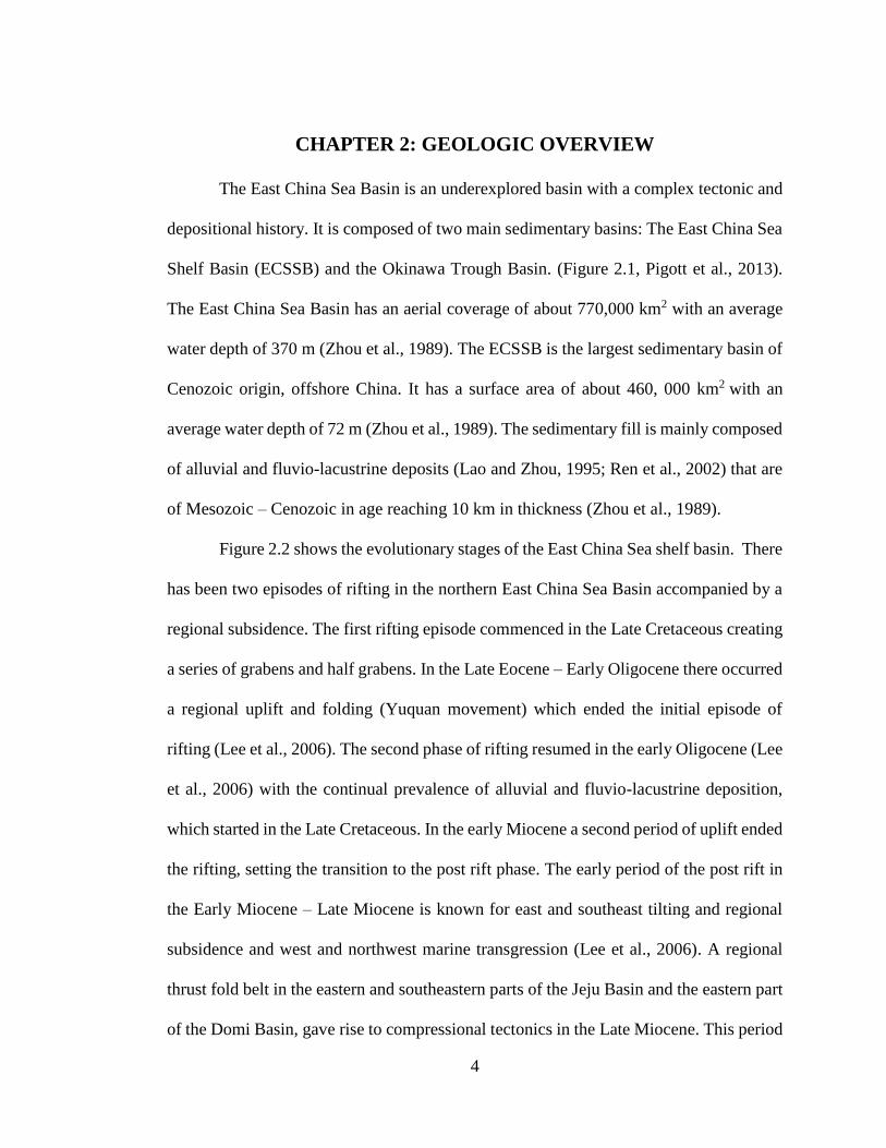
CHAPTER 2: GEOLOGIC OVERVIEW
The East China Sea Basin is an underexplored basin with a complex tectonic and
depositional history. It is composed of two main sedimentary basins: The East China Sea
Shelf Basin (ECSSB) and the Okinawa Trough Basin. (Figure 2.1, Pigott et al., 2013).
The East China Sea Basin has an aerial coverage of about 770,000 km2 with an average
water depth of 370 m (Zhou et al., 1989). The ECSSB is the largest sedimentary basin of
Cenozoic origin, offshore China. It has a surface area of about 460, 000 km2 with an
average water depth of 72 m (Zhou et al., 1989). The sedimentary fill is mainly composed
of alluvial and fluvio-lacustrine deposits (Lao and Zhou, 1995; Ren et al., 2002) that are
of Mesozoic – Cenozoic in age reaching 10 km in thickness (Zhou et al., 1989).
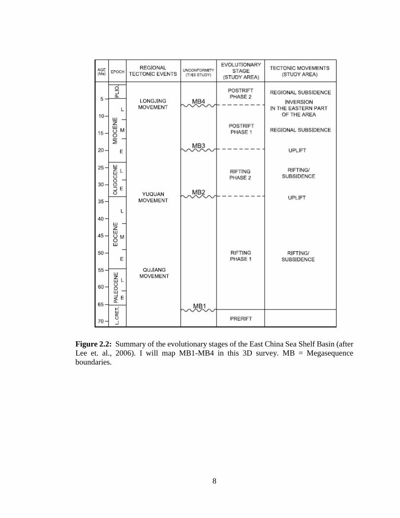
Figure 2.2 shows the evolutionary stages of the East China Sea shelf basin. There
has been two episodes of rifting in the northern East China Sea Basin accompanied by a
regional subsidence. The first rifting episode commenced in the Late Cretaceous creating
a series of grabens and half grabens. In the Late Eocene – Early Oligocene there occurred
a regional uplift and folding (Yuquan movement) which ended the initial episode of
rifting (Lee et al., 2006). The second phase of rifting resumed in the early Oligocene (Lee
et al., 2006) with the continual prevalence of alluvial and fluvio-lacustrine deposition,
which started in the Late Cretaceous. In the early Miocene a second period of uplift ended
the rifting, setting the transition to the post rift phase. The early period of the post rift in
the Early Miocene – Late Miocene is known for east and southeast tilting and regional
subsidence and west and northwest marine transgression (Lee et al., 2006). A regional
thrust fold belt in the eastern and southeastern parts of the Jeju Basin and the eastern part
of the Domi Basin, gave rise to compressional tectonics in the Late Miocene. This period

5
of inversion is referred to as the Longjing movement. Later erosion totally removed the
fold belt resulting in a prominent Late – Miocene unconformity, where majority of the
basement faults terminate. A broad continental shelf emerged which began a new episode
of regional subsidence (Lee et al., 2012).
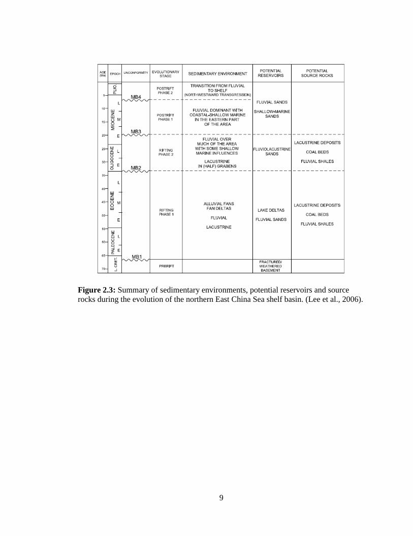
Figure 2.3 shows the environment of deposition in the East China Sea shelf basin
is mainly alluvial and fluvial. Potential reservoirs are sandstones, and source rocks are
from fluvial shales, coal and lacustrine deposits.
The Jeju Basin is an underexplored Tertiary sub basin in the north East China Sea
shelf Basin. The Jeju basin shares boundaries among three countries (Korea, Japan, and
China). The Joint Development Zone between Korea and Japan shares a boundary with
the southern region of the Jeju basin. The Jeju basin is detached from the Domi sub basin
to the north and separated from the Socotra sub basin to the south west by the Hupijiao
rise (a basement high) as shown in Figure 2.1. The Taiwan-Sinzi fold belt trending
northeast-southwest bounds the Jeju basin to the southeast (Lee et al., 2006,
Gungor,2012)
The sedimentary fill is mainly non-marine with shallow marine and shelf
sediments (Lee et al., 2006). The basin fill in the Jeju Basin ranges from less than 1500m
to greater than 4500 m in thickness , with the thinnest sediments in the central and south
western parts of the basin ( Kwon and Boggs, 2002).
The age of the sedimentary rocks in the Jeju basin range from the Oligocene to
Holocene (Kwon and Boggs, 2002) and the rocks are primarily of sandstone and
mudstone. Five depositional units define the rock strata. The first or basal unit is
composed of fluvio-lacustrine sandstone, mudstone, conglomerate and coal bed streaks

6
of Oligocene age. The second or Early to Middle Miocene unit is predominantly
sandstone and mudstone with interbedded conglomerate, coal and fresh water limestone.
The third or Late Miocene unit has stratigraphic pinch outs in some parts of the basin and
the sediments and consists of sandstones, mudstones and siltstones of fluvial input. The
fourth or Pliocene unit is composed of sandstones and mudstones with small amounts of
interbedded coal. The fifth and final or the Pleistocene- Holocene unit is majorly marine
sands and muds.

7
Figure 2.1: Structural and tectonic elements of the East China Sea. (Modified after (Zhou
et al., 1989; Yang 1992; Lee et al., 2006). HPJR = Hupijiao Rise, HJR= Haijao rise;
GYR= Gunyan Rise; YSR= Yusan rise; JB = Jeju Basin; SB = Socotra Basin;
DB = Domi Basin.
8
Figure 2.2: Summary of the evolutionary stages of the East China Sea Shelf Basin (after
Lee et. al., 2006). I will map MB1-MB4 in this 3D survey. MB = Megasequence
boundaries.
9
Figure 2.3: Summary of sedimentary environments, potential reservoirs and source
rocks during the evolution of the northern East China Sea shelf basin. (Lee et al., 2006).
10
CHAPTER 3: METHODOLOGY
DATA AVAILABLE
The Korean Institute of Geoscience and Mineral Resources (KIGAM), which is
the government of Korea’s national geological survey, acquired and provided the data.
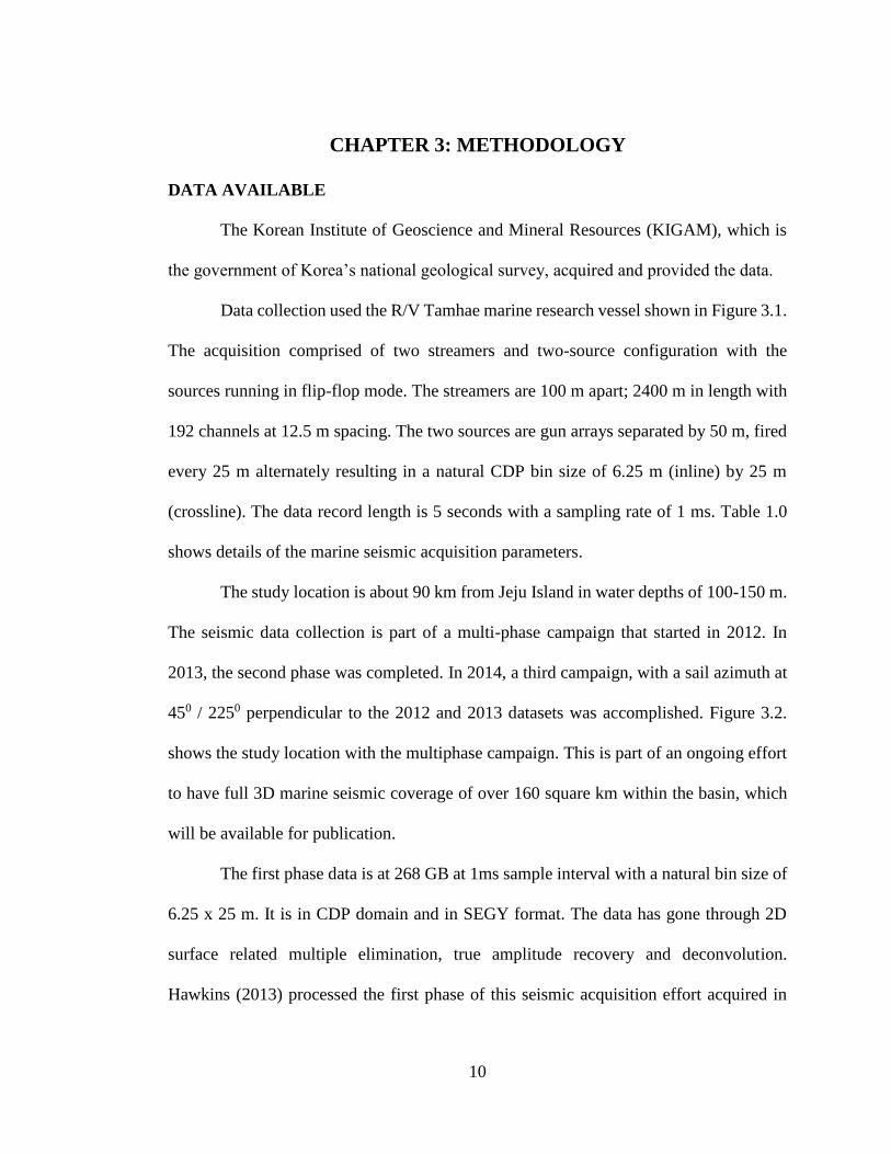
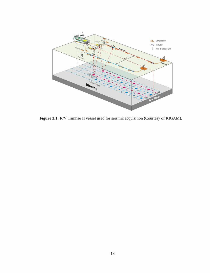
Data collection used the R/V Tamhae marine research vessel shown in Figure 3.1.
The acquisition comprised of two streamers and two-source configuration with the
sources running in flip-flop mode. The streamers are 100 m apart; 2400 m in length with
192 channels at 12.5 m spacing. The two sources are gun arrays separated by 50 m, fired
every 25 m alternately resulting in a natural CDP bin size of 6.25 m (inline) by 25 m
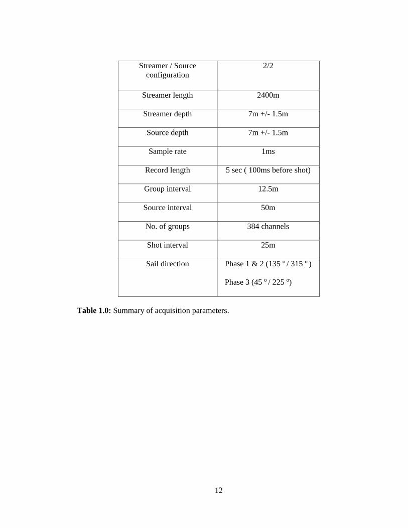
(crossline). The data record length is 5 seconds with a sampling rate of 1 ms. Table 1.0
shows details of the marine seismic acquisition parameters.
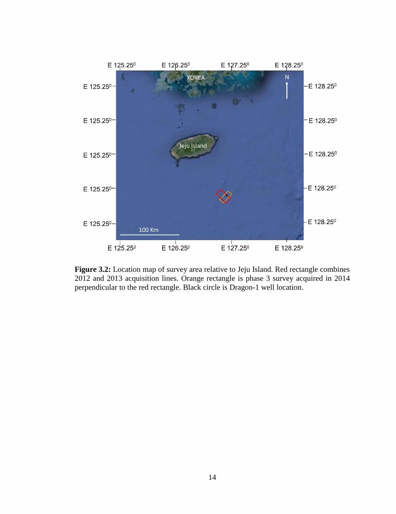
The study location is about 90 km from Jeju Island in water depths of 100-150 m.
The seismic data collection is part of a multi-phase campaign that started in 2012. In
2013, the second phase was completed. In 2014, a third campaign, with a sail azimuth at
450 / 2250 perpendicular to the 2012 and 2013 datasets was accomplished. Figure 3.2.
shows the study location with the multiphase campaign. This is part of an ongoing effort
to have full 3D marine seismic coverage of over 160 square km within the basin, which
will be available for publication.
The first phase data is at 268 GB at 1ms sample interval with a natural bin size of
6.25 x 25 m. It is in CDP domain and in SEGY format. The data has gone through 2D
surface related multiple elimination, true amplitude recovery and deconvolution.
Hawkins (2013) processed the first phase of this seismic acquisition effort acquired in

11
2012 as part of his master’s thesis. In this thesis, I process the second phase of the
acquired data and merge it with the initial phase to have a larger volume.
The second phase include raw shot gathers in SEG - D format, which consists of
51 sail lines at 268 GB, 1ms sample interval acquired in 2013, observers log and
navigation data in UKOOA P1/90 format and Dragon-1 well information. Figure 3.3
shows the 2D and 3D seismic campaign of 2012 and 2013 as well as the location of
Dragon -1 well.
12
Streamer / Source
configuration
2/2
Streamer length 2400m
Streamer depth 7m +/- 1.5m
Source depth 7m +/- 1.5m
Sample rate 1ms
Record length 5 sec ( 100ms before shot)
Group interval 12.5m
Source interval 50m
No. of groups 384 channels
Shot interval 25m
Sail direction Phase 1 & 2 (135 o / 315 o )
Phase 3 (45 o / 225 o)
Table 1.0: Summary of acquisition parameters.
13
Figure 3.1: R/V Tamhae II vessel used for seismic acquisition (Courtesy of KIGAM).
14
Figure 3.2: Location map of survey area relative to Jeju Island. Red rectangle combines
2012 and 2013 acquisition lines. Orange rectangle is phase 3 survey acquired in 2014
perpendicular to the red rectangle. Black circle is Dragon-1 well location.
15
Figure 3.3: Map showing 2D and 3D Seismic lines and Dragon -1 well location. Blue
lines were acquired in 2012 and discussed by Hawkins (2013). Red lines were acquired
in 2013. Green lines indicate locations of possible future acquisition programs. Magenta
indicates older 2D lines used to tie the Dragon well to the main area of the 3D survey. I
will integrate the 2012 and 2013 lines.
16
SEISMIC PROCESSING
Figure 3.4 shows the seismic processing workflow using a mix of commercial and
university software.
GEOMETRY DEFINITION
The SEG-D data for the phase-2 comprised of 51 sail lines. These individual lines
were imported separately into Promax. I applied the corresponding UKOOA p1/90
navigation files to each individual lines. These lines were then merged to generate a 3D
volume. I reapplied the geometry to fill in header coordinate positions for the source and
receiver. The data has a natural rectangular CDP bin size of 6.25 m x 25 m. A redefinition
to a 12.5 x 12.5 m square bin followed to correct for oversampling in the inline direction
and somewhat under sampling in the crossline direction. The maximum fold is 120 as
shown in Figure 3.5. Next, I loaded the phase-1 data and redefined the geometry to a 12.5
x 12.5 m bin. Figure 3.6 shows the fold map of the phase-1 data after geometry
redefinition to 12.5 x 12.5 m bin size, with a maximum fold of 90.
TRACE EDITING
The resulting frequencies of the phase 2 data showed little useable data above 100
Hz, indicating a safe decimation of the data to a 2 ms sample increment (where Nyquist
is 250 Hz). I decimated the phase 1 and phase 2 datasets respectively from 1ms to 2ms
using a high fidelity anti alias filter. This reduced the data size from 268 GB to 136 GB
respectively with no influence on the results, allowing for reduction in both computation
time and disk space for other processing flows. The decimated phase 2 data showed
evidence of low frequency swell noise in the shot gathers as seen in Figure 3.7a, typical
of rough weather conditions in shallow waters (Yilmaz, 2008). A band pass filter with
17
corner frequencies 8-15-80-100 Hz removed the swell noise. Next, a static shift removal
of 100 ms applied to the shot gathers due to a fixed time delay in recording before
shooting the air gun. After a static shift, I applied a top mute strategy to remove the direct
arrivals as shown in Figure 3.7b.
SURFACE RELATED MULTIPLE ELIMINATION (SRME)
The narrow azimuth (2 air gun arrays into 2 cables) geometry precludes the use
of 3D surface related multiple elimination (SRME) algorithm to suppress the multiples.
For this reason, the data preparation for the SRME thus required separating the 3D data
volume into 2D datasets based on corresponding northwest and southeast sail directions,
gun number and cable number with each sail line resulting in four 2D lines. SRME
predicts and then subtracts multiples driven by the data and does not require a model of
the subsurface. Each shot gather is a measure of the earth’s impulse response such that
one can convolve the seismic data with itself to predict multiples from primaries
(Verschuur, 2014). Multiple elimination based on SRME requires the interpolation of
traces between the zero offset and the nearest recorded hydrophone. ProMAX (and other)
SRME implementation uses an initial velocity model to define move out parameters. The
nearest trace is then interpolated along this move out parameters to approximate the data
that was not recorded. The data is now unregularized and a matching filter is calculated
and the predicted multiple is adaptively subtracted.
I picked velocities on a 1 km x 1 km grid (80 x 80 common midpoint grid) to
create the brute stack. Figure 3.8a shows the velocity semblance panel and the
corresponding CDP gather with normal moveout (NMO) applied and multiples present.
The white line in the semblance panel is the picked velocity function prior to applying

18
SRME. Note that multiples generate high stacking energy indicated by the white arrows.
It is important to avoid misinterpreting these multiples as primaries in subsequent velocity
analysis. Figure 3.8b shows the semblance panel and the same CMP NMO corrected
gather after the applying SRME with interbed and water bottom multiples suppressed.
Note the significant reduction in the stacking power of multiples in the semblance panel
Figure 3.9a shows a brute stack of the seismic data showing evidence of surface related
multiples (first and second order water bottom multiples), indicated with white arrows..
Figure 3.9b shows the same brute stack after applying SRME. Figure 3.10 shows the raw
shot gather, the predicted multiple and the shot gather after multiple suppression. I now
combined the individual multiple suppressed 2D lines back to a 3D volume.
The multiple suppressed 3D volume dataset passed through true amplitude
recovery using a 1/distance, a 6 dB/s amplitude correction factor to account for
attenuation loss and spreading wave fronts; spiking deconvolution with a prediction of 35
ms and 140 ms operator length compressed the wavelet and increased temporal
resolution. Next, I applied a scale factor of 2.314 to the phase 2 data to balance the root
means square reflection energy between phases 1 and 2.
SURVEY MERGING
I sorted the multiple suppressed SRME filtered phase 2 data into CMP gathers
and merged with the resampled phase 1 data volume, with a bin geometry of 12.5 x
12. 5 m defined. Figure 3.11 shows the fold map for the merged data. The fold map
average is about 50. Note that several spurious (non N-S trending) lines give rise to
anomalous fold. These spurious lines are due to cable feathering because of bad weather.
19
These extra data can also negatively influence the amplitude of the final imaged data
volumes.
VELOCITY ANALYSIS
Normal moveout (NMO) variations with time of the prestack gathers guide
velocity calculations. Fast velocities show an undercorrection of the reflection gathers
having a concave upward feature. Slow velocities indicate an overcorrected velocity with
reflection gathers having a concave downward feature. It is critical to have a flat gather
representing the true velocity picked at the CDP location of interest. I picked events with
high semblance that followed a geologically reasonable increase of RMS velocity with
depth. Such picking is subjective with results quality controlled by the NMO - corrected
gathers and the final stack.
The first round of velocity analysis on a 500 m x 500 m (40 x 40 common
midpoint grid ) used the semblance method. This involved generation of unmigrated super
gathers (3 inlines by 5 crosslines) with 15 common depth points (CDPS) to sum into a
gather, with a semblance sample rate of 20 ms and a calculation window of 40 ms. I
picked velocities on semblance plots, ensuring corrected flat gathers after applying
normal moveout. A smoothening of the velocity followed on every cross line and in line
at a sample rate of 2ms, and transferred to a velocity trace data on every common mid-
point. Figure 3.12 shows a representative velocity section generated and used for the first
iteration of migration.
MIGRATION
Migration focuses reflections and diffractions to their true locations. (Sheriff,
2011). Spatial resolution is increased and a more accurate seismic image of the subsurface
20
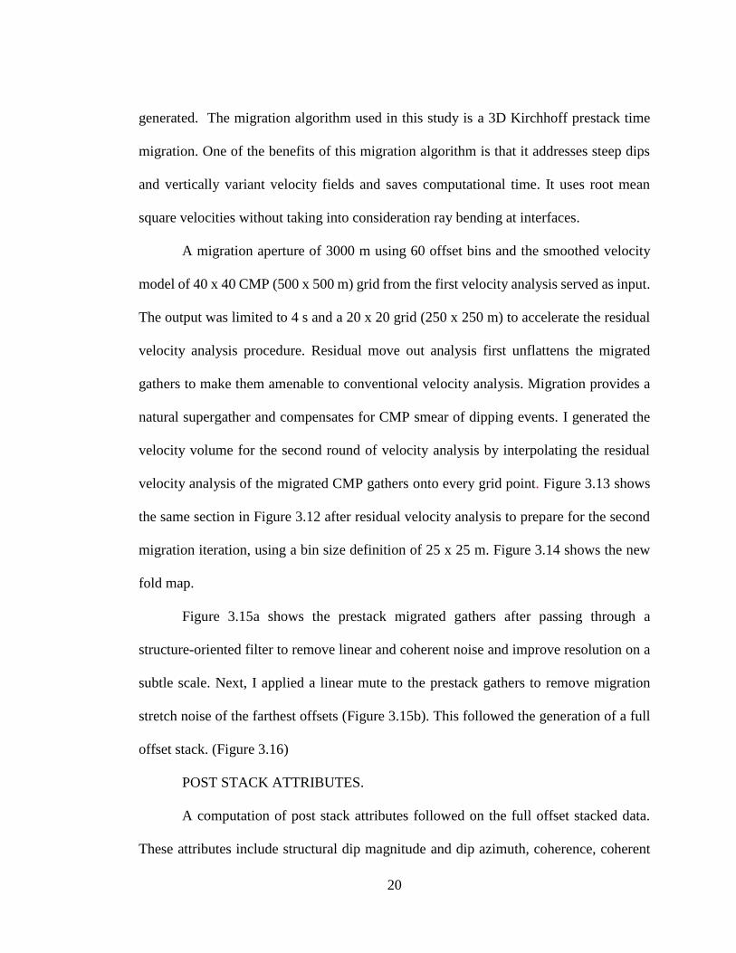
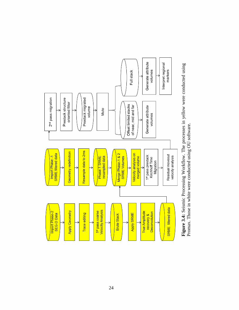
generated. The migration algorithm used in this study is a 3D Kirchhoff prestack time
migration. One of the benefits of this migration algorithm is that it addresses steep dips
and vertically variant velocity fields and saves computational time. It uses root mean
square velocities without taking into consideration ray bending at interfaces.
A migration aperture of 3000 m using 60 offset bins and the smoothed velocity
model of 40 x 40 CMP (500 x 500 m) grid from the first velocity analysis served as input.
The output was limited to 4 s and a 20 x 20 grid (250 x 250 m) to accelerate the residual
velocity analysis procedure. Residual move out analysis first unflattens the migrated
gathers to make them amenable to conventional velocity analysis. Migration provides a
natural supergather and compensates for CMP smear of dipping events. I generated the
velocity volume for the second round of velocity analysis by interpolating the residual
velocity analysis of the migrated CMP gathers onto every grid point. Figure 3.13 shows
the same section in Figure 3.12 after residual velocity analysis to prepare for the second
migration iteration, using a bin size definition of 25 x 25 m. Figure 3.14 shows the new
fold map.
Figure 3.15a shows the prestack migrated gathers after passing through a
structure-oriented filter to remove linear and coherent noise and improve resolution on a
subtle scale. Next, I applied a linear mute to the prestack gathers to remove migration
stretch noise of the farthest offsets (Figure 3.15b). This followed the generation of a full
offset stack. (Figure 3.16)
POST STACK ATTRIBUTES.
A computation of post stack attributes followed on the full offset stacked data.
These attributes include structural dip magnitude and dip azimuth, coherence, coherent
21
energy, Sobel filter, gradient components, and most positive and most negative curvature
volumes. The structural dip computation used a modification of the Kuwahara filter using
a 5 x 5-multi analysis-running window (Marfurt 2006). The seismic amplitude is used as
input.
Dip Magnitude and Dip Azimuth
Volumetric dip measures correspond to a plane that best fits the trend of the
adjacent traces. Dip magnitude and azimuth maps can reveal subtle faults and
stratigraphic features that are present because of differential compaction and waveform
changes (Chopra and Marfurt 2007). Changes in dip and azimuth can aid in understanding
sequence stratigraphic framework as seen from termination of reflection patterns (Chopra
and Marfurt 2007).
Sobel Filter Similarity
Luo et al. (1996) introduced this filter applicable to seismic data. It is an amplitude
sensitive multi trace attribute. Derivatives are computed along inline and crossline
amplitude along reflector dip and azimuth within a vertical analysis window. The Sobel
filter is the magnitude of this amplitude gradient vector (Chopra and Marfurt 2007). The
Sobel Filter is sensitive to both thin bed tuning and changes in waveform, thus
highlighting channels, faults and lineaments
Coherent energy & coherent energy gradient components
Coherent energy and coherent energy gradients are computed from the first
principal components of the seismic waveforms in an analysis window. Physically, the
first principal components provides the waveform that best fits the data. (Marfurt 2006).
The principal component is that part of the data that can be represented by this single
22
waveform. The coherent energy gradient measures the amplitude variability of the
coherent component of the seismic data along structure (Chopra and Marfurt, 2007). It
highlights stratigraphic features (channels) with a higher definition, lower than the tuning
thickness and provides insights into reservoir heterogeneity (Chopra and Marfurt 2007).
Curvature
Curvature attributes can enhance subtle information not visible using dip-
magnitude and dip-azimuth attributes (Chopra and Marfurt 2012). Curvature is the
inverse of the radius of a circle tangent to a curve. Anticlines exhibit positive curvature,
synclines a negative curvature and planes zero curvature for planes (Chopra and Marfurt
2007). Volumetric curvature show areas of flexures, folds, collapse features, lineaments
and channel evidence if differential compaction is present (Chopra and Marfurt 2007).
Most positive (K1) and most negative (K2) were derived.
After the generation of the respective attributes, an export of these attributes and
seismic amplitude volumes into segy format for interpretation using a commercial
software package.
PRESTACK ATTRIBUTES
The response of the seismic signal changes with offset (AVO) due to changes in
lithology, porosity, density and fluid indicators. In general, structural and stratigraphic
effects exist at near stacks while far stacks show lithological and fluid effects. Such
amplitude versus offset (AVO) effects will help delineate reservoir heterogeneity,
volcanic intrusions, coal, and possible hydrocarbon presence.
Figure 3.18 shows the workflow for prestack attribute generation. I generated
offset limited volumes of the near, mid and far stacks, with an offset interval of 800m.

23
The near stack ranged from 125 - 925 m, the mid stack from 925 - 1725 m and the far
stack from 1725 - 2525 m, using the prestack migrated gathers with the prestack structure
oriented filter applied. I computed coherent energy attribute for the offset limited volumes
and created time slices to study the effects of amplitude variations with offset for each
substack.
24
Fig
ure
3.4
: S
eism
ic P
roce
ssin
g W
ork
flow
. T
he
pro
cess
es i
n y
ello
w w
ere
conduct
ed u
sing
Pro
max
. T
hose
in w
hit
e w
ere
conduct
ed u
sin
g O
U s
oft
war
e.
25
Figure 3.5: Fold map for seismic data of phase 1 with bin size of 12.5 x 12.5 m. Crooked
lines are due to bad weather
26
Figure 3.6: Fold map for seismic data of phase 2 with bin size of 12.5 x 12.5 m.
27
Figure 3.7: (a) Raw raw shot gather showing low frequency swell noise curtain, (b) The
same raw shot gathers shown in (a) after applying a band pass filter to suppress the swell
noise. Note the removal of swell curtain. A static shift of 100 ms and a top mute applied
to remove the direct arrival.

28
Fig
ure
3.8
: (a
) V
eloci
ty s
embla
nce
pan
el w
ith n
orm
al m
ove
out
(NM
O)
appli
ed t
o c
om
mon d
epth
poin
t (C
DP
)
gat
her
s bef
ore
SR
ME
. T
he
whit
e li
ne
is t
he
pic
ked
vel
oci
ty f
unct
ion u
sed p
rior
to S
RM
E.
Whit
e ar
row
s in
dic
ate
regio
n w
ith m
ult
iple
s. (
b)
Vel
oci
ty s
embla
nce
pan
el w
ith N
MO
appli
ed t
o C
DP
gat
her
s af
ter
SR
ME
. N
ote
the
reduct
ion i
n t
he
stac
kin
g p
ow
er o
f th
e m
ult
iple
s.
29
Fig
ure
3.9
: (a
) B
rute
sta
ck w
ith m
ult
iple
s in
dic
ated
by w
hit
e ar
row
s. (
b)
Bru
te S
tack
aft
er m
ult
iple
suppre
ssio
n
usi
ng S
RM
E.
30
Fig
ure
3.1
0:
(a)
Raw
sh
ot
gat
her
s (b
) S
RM
E p
redic
ted m
ult
iple
s (c
) S
hot
gat
her
s af
ter
SR
ME
.
31
Figure 3.11: Fold map of merged survey – Phase 1 and Phase 2. The fold average is about
60. Several spurious (non N-S trending) lines give rise to anomalous fold

32
Fig
ure
3.1
2:
A r
epre
sen
tati
ve
ver
tica
l sl
ice
thro
ugh
th
e 3
D v
elo
city
mo
del
use
d f
or
the
firs
t it
erat
ion
of
pre
stac
k t
ime
mig
rati
on
.
33
Fig
ure
3.1
3:
A r
epre
sen
tati
ve
ver
tica
l sl
ice
thro
ugh
th
e 3
D v
eloci
ty m
od
el a
fter
on
e it
erat
ion
of
pre
stac
k
tim
e m
igra
tion a
nd r
esid
ual
vel
oci
ty a
nal
ysi
s (f
orm
ing a
ste
p i
n t
he
Der
ego
wsk
i lo
op
).
34
Figure 3.14: Fold map of the merged survey at the migration bin size of 25 x 25. Later
migrations may be computed at a denser bin size if data quality permits. Later iterations will
also remove irregular (curved) seismic lines which will give rise to local amplitude artifacts.
Average fold is about 120.
35
Figure 3.15: (a) A representative migrated gather after prestack structured oriented
filtering. Note the primaries are quite flat. The hockey sticks in the shallow section can
be addressed using nonhyperbolic moveout. Multiples remain in the basement below
2.5s. (b) The same migrated gather after muting to minimize the negative impact of
nonhyperbolic moveout and migration stretch.
36
Figure 3.16: Full stack representative seismic amplitude section.
37
Fig
ure
3.1
7:
Work
flow
for
gen
erat
ing p
rest
ack a
ttri
bute
s.
38
CHAPTER 4: DATA ANALYSIS AND INTERPRETATION
The final stacked section showed different structural and stratigraphic features
with varying anomalous amplitudes due to cable feathering from bad weather conditions.
These anomalous amplitudes are still evident after performing residual velocity analysis
as suggested by Hawkins (2013) and prestack structure oriented filtering. Figure 4.1
shows a coherent energy seismic section. Note the anomalous amplitudes in white arrows
at the shallow sections due to cable feathering. Figure 4.2 shows the Sobel filter similarity
section better imaged the faults. Figure 4.3 shows a co-rendered image of most positive
curvature (K1) in red, most negative curvature (K2) in blue and seismic amplitude. There
is a correlation of structural highs to anticlinal features and structural lows to synclines
and down thrown fault blocks. These attributes guided interpretation of faults and
mapping of reflections that correspond to mega sequence boundaries identified by Lee et
al. (2006) and Cukur et al. (2011).
I identified and mapped five horizons and generated time maps. These five
horizons correspond to four mega sequence boundaries (MB) namely: MB1, MB2, MB3,
MB4 and the sea floor. MB 1 is the oldest of the mega sequence boundaries in geologic
age. Figure 4.4 shows the interpreted faults and mapped mega sequence boundaries.
STRUCTURE OF MEGASEQUENCE BOUNDARIES AND SEAFLOOR
Normal faults are present in the study area. Most of these faults are basement
induced. The faults are normal and exhibit elements of growth. The faults have a regional
southeast dip with a northeast-southwest trending strike. Antithetic faults with
northwesterly dips and strikes trending northeast - southwest are also present. Structures
39
described include broad anticlinal, fault dependent structures. Roll over anticlines appear
against downthrown fault blocks. Horst, half graben and graben features are present.
MEGA SEQUENCE BOUNDARY (MB1)
Figure 4.5 shows the time structure map of MB1. The geologic age is Late
Cretaceous and forms the top of the acoustic basement. The two-way travel time interval
ranges from 1680 to 2750 ms. It consists of half graben, graben and horst features. The
faults are normal and basement induced. The basement faults divide the study area into
several fault compartments. The faults trend northeast - southwest and dip to the
southeast. This trend follows the regional trend of faults in the north East China Sea
Basin. The faults show high displacement of reflections across faults. There is a high
displacement of reflections across the faults, and is synonymous with a period of rifting
that occurred in the north East China Sea shelf basin.
MEGASEQUENCE BOUNDARY (MB2)
Figure 4.6 shows the time structure map for MB2. The geologic age is Late
Eocene – Early Oligocene; basement faults cut through this mega sequence boundary.
The range of values in two way travel time is from 1370 to 1730 ms. Roll over anticlines
exist on the hanging wall block. The highest relief is to the northwest. The fault throws
are less than those seen MB1. MB2 overlies an angular unconformity in some parts of the
survey.
MEGASEQUENCE BOUNDARY (MB3)
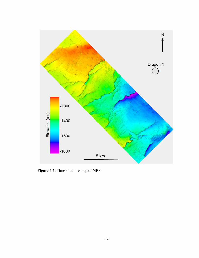
Figure 4.7 shows the time structure map for mega sequence boundary 3. The
geologic age is Early Miocene. The time ranges from 1240 to 1610 ms. The highest relief
is in the northwestern region, with relief decreasing southwards. The time structure map

40
is similar to MB2. Antithetic / conjugate faults are present at this interval. The faults are
also normal faults with a northeast - southwest strike compartmentalizing the sequence
boundary. The basement faults cut through this boundary as well. Roll over anticlinal
structures terminate against downthrown compartments of the fault blocks.
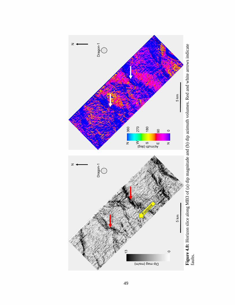
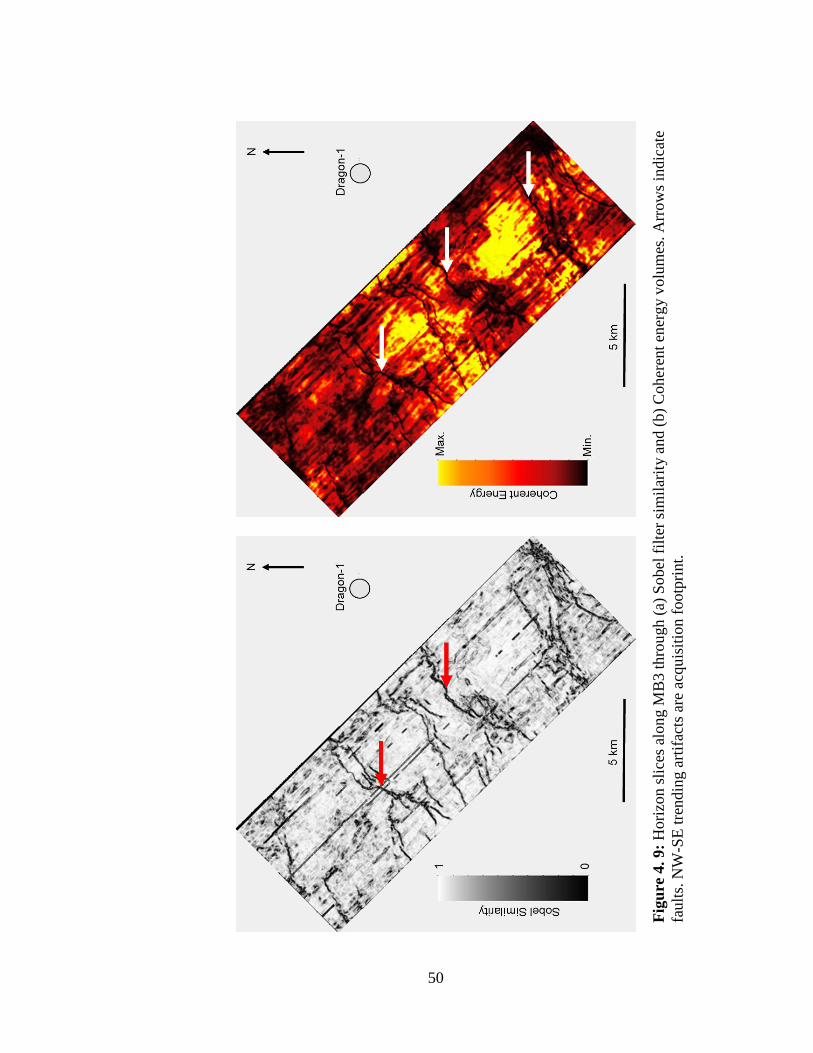
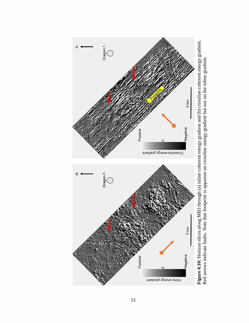
I also extracted horizon slices of dip magnitude & dip azimuth, Sobel filter,
coherent energy, inline energy and crossline energy gradients and most positive and most
negative curvature along the MB3 horizon. Figure 4.8a shows the dip magnitude map and
Figure 4.8b shows the azimuth map. Figure 4.9a shows the Sobel filter and Figure 4.9b
the coherent energy. Figure 4.10a and b shows inline energy gradient and crossline energy
gradient. Figure 4.11a shows most positive curvature and Figure 4.11b shows most
negative curvature. The attributes shows the fault compartmentalization within the study
area. The attributes exacerbate the acquisition footprint and appear as northwest-southeast
lineations.
MEGASEQUENCE BOUNDARY (MB4).
Figure 4.16 shows the time structure map of MB4. The geologic age is Late
Miocene. It has a flat lying geology overlain by a broad subtle low relief anticline. The
top of this anticline is eroded, inferring a period of non - deposition and erosion creating
angular unconformities at the limbs. The angular unconformities are to the northwest and
southeast respectively. This is a post rift phase called the Longjing movement. It is a time
of structural inversion where reverse faulting occurred. However, reverse faults are not
noticeable in the data. Zhou et al. (1989), Lee et al. (2006) and Lee et al. (2012) described
this prominent unconformity. The time ranges from 560 to 750 ms. Faults are least
predominant at this level, with less throw across reflections and few basement faults

41
cutting, due to a period of inversion in the Late Miocene and fault reactivation identified
by Lee et al. (2006).
SEAFLOOR
Figure 4.17 shows the time structure map for the seafloor, ranging from 130 to
210 ms. It has a relatively gentle relief. A topographic low is present that trends northwest
to southeast with a time range from 190 to 210 ms, bounded by two structural highs. The
structural high to the south has a larger surface area with two-way travel times ranging
from 120 to 150 ms. It shows an undulating relief in the north south direction.

42
Figure 4.1: Coherent energy section showing anomalous high coherence indicated by
white arrows. These anomalies are not geological but due to cable feathering. Blue arrows
indicate high amplitude anomalies that are geologically reasonable.
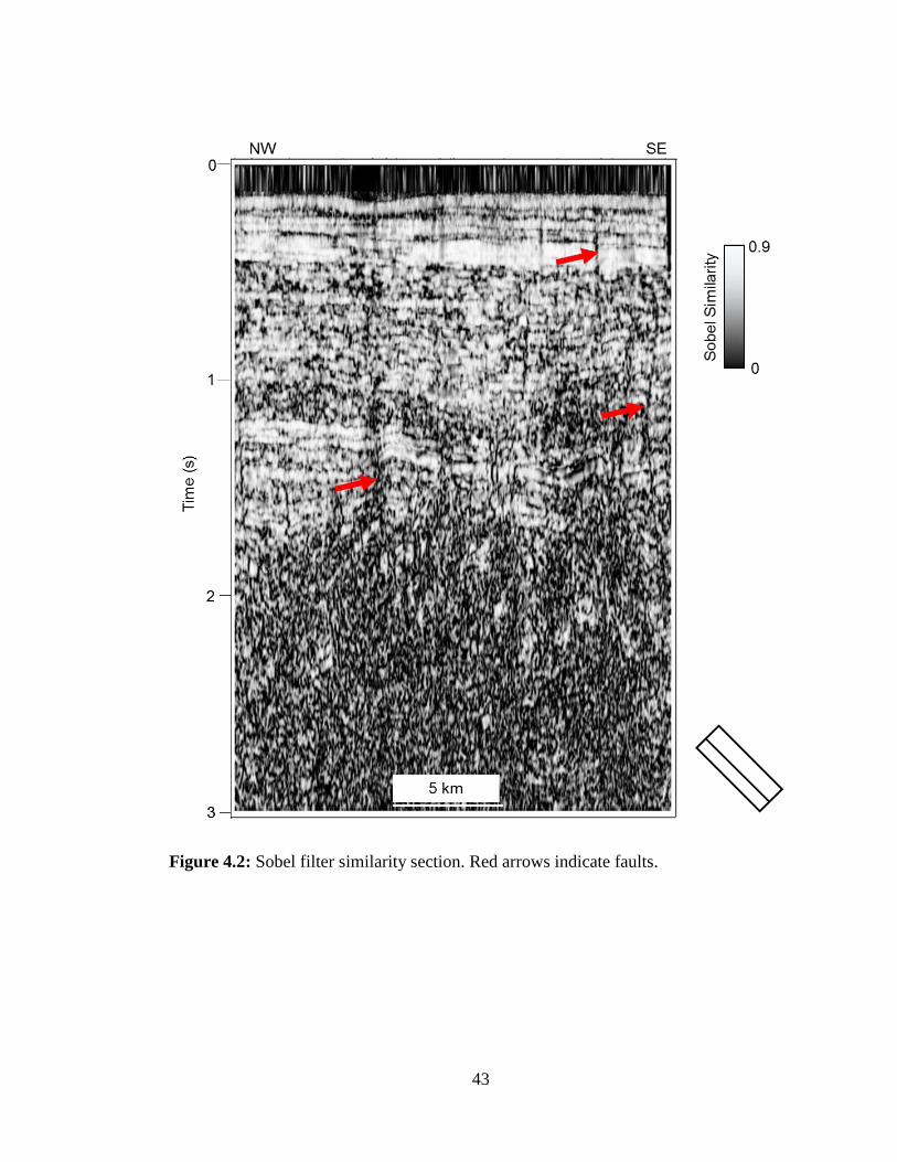
43
Figure 4.2: Sobel filter similarity section. Red arrows indicate faults.

44
Figure 4.3: Seismic amplitude co-rendered with most positive curvature in red and
most negative curvature in blue.
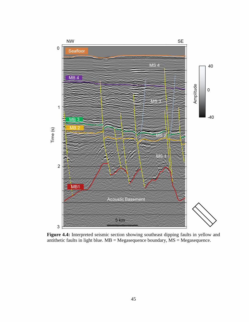
45
Figure 4.4: Interpreted seismic section showing southeast dipping faults in yellow and
antithetic faults in light blue. MB = Megasequence boundary, MS = Megasequence.

46
Figure 4.5: Time structure map of MB1.
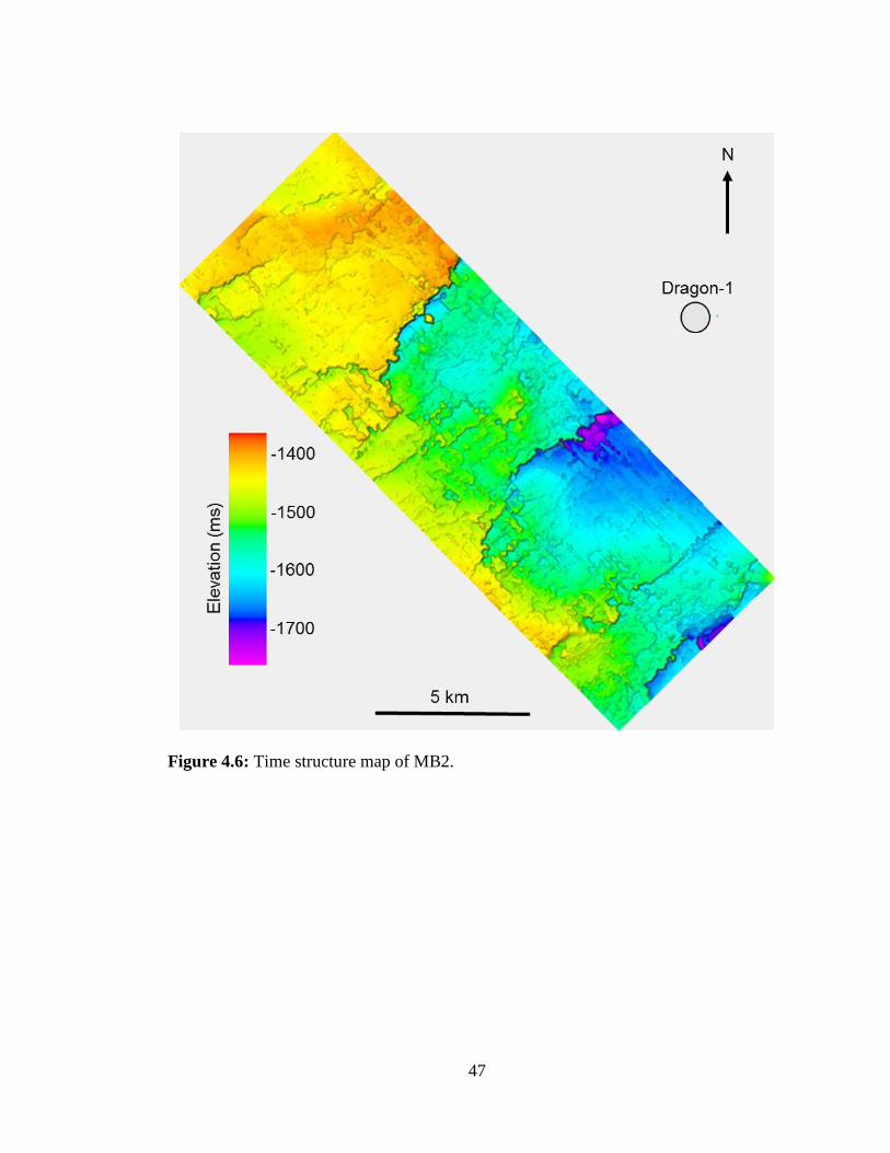
47
Figure 4.6: Time structure map of MB2.
48
Figure 4.7: Time structure map of MB3.
49
Fig
ure
4.8
: H
ori
zon s
lice
alo
ng M
B3 o
f (a
) dip
mag
nit
ude
and (
b)
dip
azi
muth
volu
mes
. R
ed a
nd w
hit
e ar
row
s in
dic
ate
fault
s.
50
Fig
ure
4. 9:
Hori
zon s
lice
s al
on
g M
B3 t
hro
ugh (
a) S
obel
fil
ter
sim
ilar
ity a
nd (
b)
Coher
ent
ener
gy v
olu
mes
. A
rrow
s in
dic
ate
fault
s. N
W-S
E t
rendin
g a
rtif
acts
are
acq
uis
itio
n f
ootp
rint.
51
Fig
ure
4.1
0:
Hori
zon s
lice
s al
ong M
B3 thro
ugh
(a)
inli
ne
coher
ent en
erg
y g
radie
nt an
d (
b)
cro
ssli
ne
coh
eren
t en
erg
y g
rad
ien
t.
Red
arr
ow
s in
dic
ate
fault
s. N
ote
that
footp
rint
is a
ppar
ent
on c
ross
line
ener
gy g
radie
nt
but
not
on t
he
inli
ne
gra
die
nt.
52
Fig
ure
4.1
1:
Hori
zon
sli
ces
along M
B3 thro
ugh
(a)
most
posi
tive
curv
ature
(K
1)
and (
b)
most
neg
ativ
e cu
rvat
ure
(K
2).
Note
the
nort
hw
est
south
east
lin
eati
on i
s due
to a
cquis
itio
n f
ootp
rint.
Arr
ow
s in
dic
ate
fault
s.
53
Figure 4.12: Time structure map of MB4.
54
Figure 4.13: Time structure map of the sea floor.

55
STRATIGRAPHY OF MEGASEQUENCES
I describe four mega sequences (MS) originally described on 2D data by Lee et
al. (2006) and Cukur et al. (2011) namely: MS1, MS2, MS3 and MS4 where MS 1 is the
oldest and MS 4 is the youngest. The mega sequences (MS) are defined by two adjacent
mega sequence boundaries (MB). I created isochron maps for each of the four mega
sequences, to understand the thickness changes and spatial distribution of sediments. I
observe that the location of the maximum thickness for each sequence increased from the
north for the oldest sequence to the south for the youngest sequence. Figure 4.14 shows
an interpreted seismic amplitude section of mega sequences with stratigraphic and
structural features identified.
MEGASEQUENCE ONE (MS 1)
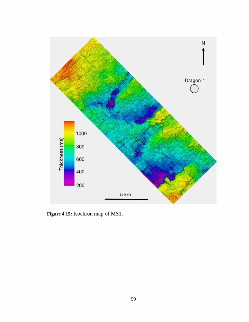
Figure 4.15 shows the isochron map for MS1, defined as the numerical difference
between MB1 and MB2. The base of the sequence is the top of the acoustic basement
with chaotic reflections below the acoustic basement. The top of the acoustic basement
showed high amplitudes representative of the acoustic basement. It is the thickest of the
four-mega sequences with isochron values greater than 1000 ms. The region with the
maximum thickness is in the northwest of the study area. Reflections vary from low to
variable to high amplitudes. Moderate to high amplitudes irregular reflections to the base
of MS1 may be indicative of volcanic flows. Localized high amplitudes (bright spots) are
apparent terminating against upthrown fault blocks. These high amplitudes could be
indicative of volcanic intrusions, coal or hydrocarbons. Divergent beds with steep dips
are found in half grabens and grabens. The divergent beds indicate differential subsidence
synonymous with synrift tectonism. The beds thicken away from the footwall fault block

56
towards the adjacent downthrown fault block. These divergent beds are interpreted as
alluvial fans (Kwon and Boggs, 2002). The stratigraphy is composed of alluvial fan and
fan deltas, lacustrine and fluvial channels with thin coal beds lying conformably on each
other (Kwon and Boggs, 2002).
MEGASEQUENCE TWO (MS2)
Figure 4.16 shows the isochron map for MS2. This is the defined as the numerical
difference between MB2 and MB3. It has the lowest thickness among the mega
sequences, of about 300ms. The reflections are low to medium amplitude with a degree
of continuity. Divergent reflections also exist in this sequence. They do not show as much
dip, and are less pronounced when compared to MS1. The sediments are mainly fluvial
channels and flood plains in origin.
MEGASEQUENCE THREE (MS3)
Figure 4.17 shows the isochron map for MS3. This is the difference in time
between MB4 and MB3. Isochron thickness is greater than 900 ms. The region with the
maximum thickness is more distal when compared to the maximum thicknesses seen in
MS1 and MS2. An angular unconformity exists to the southeast. The angular
unconformity to the southeast shows more dip. A broad anticline exists only in this
sequence and is associated with a period of structural inversion. An erosional truncation
that is a period of non-deposition describes the top of the sequence, and overlies the top
of the anticline. This period of non-deposition and erosion creates angular unconformities
at the anticlinal limbs. Angular unconformities are seen to the northwest and southeast,
with the angular unconformity to the southeast showing a greater dip. The reflections
show sub parallel bedding with low, variable and high amplitudes with varying degrees

57
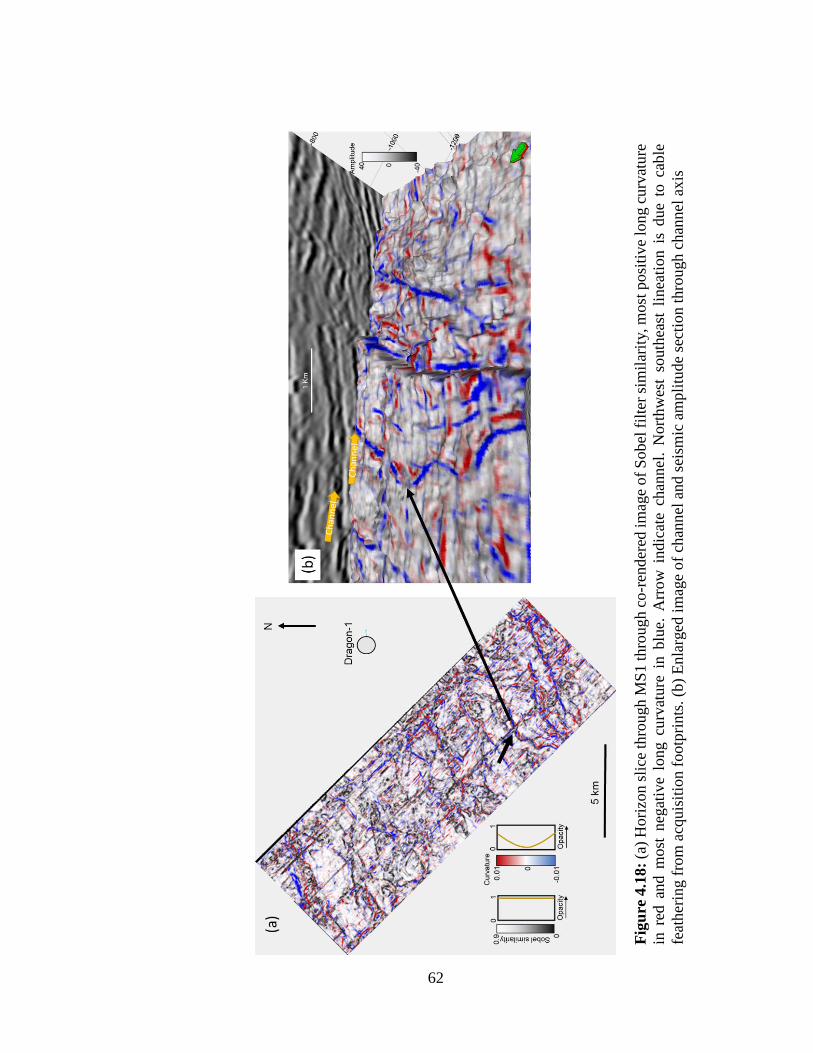
of continuity. It is a period of post deposition / post rift. Figure 4.18 shows a horizon slice
through the Sobel filter co-rendered with K1 and K2 curvature volumes, showing channel
features identified in this sequence. I interpret the channels to be clay filled due to their
negative curvature expression. In contrast, the channel banks exhibit a most positive
curvature and may be sand rich, perhaps a point bar.
MS3 consists of siltstone, sandstones and clay stones with minor coal beds.
(Kwon and Boggs, 2002). Deposition is predominantly a fluvial environment.
MEGASEQUENCE FOUR (MS4)
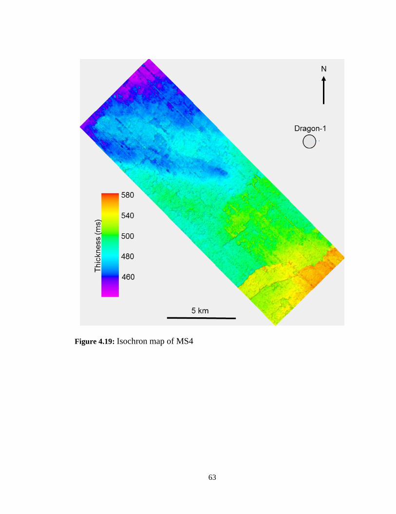
Figure 4.19 shows the isochron map for MS4. This is the numerical difference in
between MB 4 and the seafloor. The reflections show parallel bedding and reflection
continuity. MS 4 is subdivided into two units, with a strong continuous reflection that
separates the upper and lower unit. The upper unit ranges from the sea floor – 400 ms
two-way time exhibiting low to variable amplitudes. The environment of deposition for
this unit is shallow marine, composed of unconsolidated sands and muds (Kwon and
Boggs, 2002). The lower unit reflections exhibit reflection discontinuities with varied
amplitudes. The basal part of the lower unit shows more reflection discontinuities, which
may be representative of channelization from non-marine sources.
58
Figure 4.14: Seismic amplitude section showing mega sequences (MS) with divergent
beds, channels, bright amplitudes identified within the megasequences.
59
Figure 4.15: Isochron map of MS1.

60
Figure 4.16: Isochron map of MS2.

61
Figure 4.17: Isochron map of MS3.
62
Fig
ure
4.1
8:
(a)
Hori
zon s
lice
thro
ugh M
S1 t
hro
ugh c
o-r
end
ered
im
age
of
Sobel
fil
ter
sim
ilar
ity, m
ost
posi
tive
long c
urv
ature
in r
ed a
nd m
ost
neg
ativ
e lo
ng c
urv
ature
in b
lue.
Arr
ow
indic
ate
chan
nel
. N
ort
hw
est
south
east
lin
eati
on i
s due
to c
able
feat
her
ing f
rom
acq
uis
itio
n f
ootp
rints
. (b
) E
nla
rged
im
age
of
chan
nel
and s
eism
ic a
mpli
tude
sect
ion t
hro
ugh c
han
nel
ax
is
63
Figure 4.19: Isochron map of MS4
64
AMPLITUDE ANALYSIS OF OFFSET LIMITED STACKS.
While picking the sequence boundaries, I noticed high amplitudes terminated
against fault blocks. I used offset limited sub stacks to investigate amplitude variation
with offset (AVO). Figures 4.20, 4.21 and 4.22 shows the near, mid and far stacks. The
missing sections in the mid and far stacks is due to a short offset distance of 2400m. This
also constrained the horizon slice created to MS1 to study the changes in AVO effects
due to lithology and fluid effects on a spatial scale. I tracked amplitude changes using the
orange, blue and yellows arrows as a guide as shown on the seismic amplitude section of
the sub stacks as shown in Figures 4.20, 4.21 and 4.22. There is a varied increase in
amplitude from the near to the far stack. Improved resolution and continuity on the far
stack in imaging the acoustic basement is apparent when compared to the near and mid
stack. This assisted in the interpretation of the acoustic basement (MB1). These bright
spots show positive reflections.
I generated a horizon slice within MS1 through near, mid and far stacks of coherent
energy as shown in Figure 4.23. I see higher amplitudes on the mid stack than the near
and far stack. I also generated a horizon slice through MB1 of coherent energy for the sub
stacks (Figure 4.24) to ascertain if I obtain the same amplitude response with the mid
stack. However, the far stack showed higher amplitudes than both the near and mid stacks.
By comparing the two amplitudes, it shows that there is a difference in lithology between
the horizon slice extracted within MS1 and MB1 the acoustic basement.
These increased amplitudes seen on the far stack may be due to igneous activity as
noted by Cukur et al. (2011) by wells drilled in some of the strong amplitudes seen on 2D
data or caused by wet sands as evident by wells drilled in the basin (KIGAM, 1997).

65
Amplitude anomalies may also be due to coal deposits as reported in the Pinghu area (Lee
et al., 2006).
66
Figure 4.20: Near stack (125 - 925 m). Orange and red arrows show low amplitudes.
Blue arrow shows high amplitude.
67
Figure 4.21: Mid stack (925 - 1725 m). Orange arrow shows moderate amplitude
compared to near stack, blue arrow lower amplitude than near stack. Red arrow reveals
moderate amplitude anomalies.
68
Figure 4.22: Far stack (1725 - 2525 m). Orange arrow shows higher amplitudes
compared to near and mid offset stack. Note the saucer shape; this may be a volcanic sill
or velocity pull down due to gas effect. Blue arrow shows increased amplitude compared
to the near stack. Red arrow reveals high amplitude anomalies greater than the near and
mid stack.
69
Figure 4.23: Horizon slice of coherent energy through (a) near stack, (b) mid stack, (c)
far stack, and (d) full stack. Black arrows indicate regions with change in amplitude
anomalies. Note that the mid stack shows higher amplitudes than the near and mid stack.
(e) Representative seismic section showing horizon in white dotted lines used to generate
horizon slice through near, mid, far and full stack.
70
Figure 4.24: Horizon slices along MB1 through coherent energy of (a) near stack, (b)
mid stack, (c) far stack, and (d) full stack. Black arrows indicate regions with changes in
amplitude anomalies. Note that the farstack shows higher amplitudes than the near and
mid stack. Note no amplitudes are seen on the near stack.

71
IMPLICATIONS FOR HYDROCARBON PROSPECTIVITY
Multiple traps that could hold hydrocarbons are seen in the study area. These
include: (a) broad anticlinal traps, (b) structures against upthrown fault blocks, and (c)
erosional truncations, angular unconformities and channels. The anticlinal traps observed
in MS3 form hydrocarbon traps in Xihu depression, where Chen and Ge (2003) noted
that a greater percentage of the hydrocarbon volume are associated with inversion
structures. These anticlinal traps may also trap hydrocarbons as evident from the Xihu
depression. These inversion structures have been the focus of major exploration efforts
in the basin. They also have the lowest risk from an exploration standpoint. The structures
against upthrown fault blocks and roll over anticlines are apparent in MS1. The erosional
truncations, angular unconformities and channels seen in MS3 may serve as stratigraphic
traps.
Source rocks that could generate hydrocarbon are found in lacustrine shales,
fluvial shale and coal beds synonymous with the rifting phase. Silverman et al. (1996)
noted that source rocks are thermally mature interbedded organic rich shales as seen in
the Ping Hu field. Source rocks in the study area could possibly expel oil and gas into the
fault traps and rollover anticlines if they are mature. Faults could also act as conduits for
migration of oil into the broad anticlinal structure in MS3. I hypothesize that traps buried
at depth will be closer to the hydrocarbon window. Exploration of these traps has not yet
occurred and there is a likelihood of trapping oil and gas.
Anomalous bright amplitudes terminate against footwall fault blocks. These
amplitudes do not cut across the faults suggesting that if the amplitudes are due to
hydrocarbons that these faults will be sealing and will serve as potential traps for

72
hydrocarbon accumulation. These amplitudes could be indicative of hydrocarbons, with
the amplitudes dying out at the trap edge, or maybe coal, wet sands or volcanic
emplacement.
Potential reservoirs are fluvial and littoral sandstones that are Eocene in age that
produce gas and condensate while oil production is from Oligocene interbedded
sandstone, siltstone and mudstone of fluvial and lacustrine origin as observed by
Silverman et al. (1996) in the Ping Hu field. Channel deposits seen in MS3 could serve
as reservoirs and also fluvial, lacustrine and fan deltas in MS1 and MS2.
The timing, generation and migration of hydrocarbon from source rocks and trap
formation is critical for hydrocarbon in place when prospecting within this traps.
Hydrocarbons produced before trap creation may not hold hydrocarbons or show residual
oil while hydrocarbons generated during or after trap formation will have a higher
probability of trapping hydrocarbon and will be prospective zones for future exploration.
73
CHAPTER 5: CONCLUSIONS
Key processing steps for the 160 km2 Jeju survey included resampling to 2ms and
bandpass filtering to remove swell noise observed in the data. 2D surface related multiple
elimination suppressed multiples in the brute stack; deconvolution and true amplitude
recovery increased temporal resolution and balanced the amplitude. A merger of the 2013
phase 2 data with the 2012 phase 1 dataset increased the migration aperture. Velocity
analysis and residual velocity analysis on the merged volume prepared the data for
prestack Kirchhoff time migration. Prestack structure-oriented filtering reduced linear
and coherent noise applied on the final prestack migrated gathers. The gathers were
stacked into full and partial stacks of near, mid and far offsets. The stacked section
showed the data is of good quality although anomalous amplitudes are seen in the shallow
sections caused by cable feathering.
Geometric attributes including Sobel filter similarity, curvature, coherent and
coherent energy gradient were generated on the full stack. Similarity attributes
accentuated channel edges and faults. Curvature attributes delineated structural highs
such as roll over anticlines for the most positive curvature and structural lows such as
differential compaction over channels. Positive and negative curvature anomalies
straddled major faults. Coherent energy showed areas with anomalous amplitudes. All
these attributes exacerbated acquisition footprint.
Basement-induced faults trending northeast southwest are associated with broad
anticlines, rollover anticlines, fault dependent structures, graben and half graben features
and horst structures. Stratigraphic features such as divergent beds indicate synrifting in
MS1 and MS2, parallel and sub parallel beds in MS3 and MS4 are associated with a more

74
quiescent post rift phase. Four mega sequence boundaries (MB) in the study area
previously reported on 2D data in other parts of the north East China Sea are identified.
Time maps of MB1, MB2, MB3, MB4 and the sea floor show variability in the faulting
architecture and structural relief. Isochron maps of the four-mega sequences (MS) show
maximum thickness increased from proximal to distal from the oldest to the youngest
sequences.
Prestack amplitude attributes of the offset limited stacks on seismic sections
showed increased amplitudes on the far offset stack. The far offset stack showed a better
definition of the basement configuration; this allowed for confident interpretation of the
acoustic basement. A horizon slice of the near, mid and far stacks through coherent energy
within MS1 reveals that the mid stack showed higher amplitudes than the near and far
stack. This is different from observations of a horizon slice of MB1 through coherent
energy of the near, mid and far stacks. The far offset stack showed the higher amplitudes
than the near and mid stacks. These varied amplitudes seen on these horizon slices may
be indicative of volcanic intrusions, wet sands, coal or possible hydrocarbons. It also
suggests that the lithology closer to the basement is different from the other lithologies
overlying it.
Possible targets for hydrocarbon exploration include rollover anticlines, fault
dependent structures and bright amplitudes terminating against faults, which are
dependent on timing of oil generation, migration pathway, seal, reservoir rock and source
rock.
Incorporation of the phase-3 program promises to incorporate the Dragon-1 well.
This will assist in calibrating the well lithology to seismic to establish a robust

75
understanding of amplitude variation with offset. The next stage of processing will
directly address the artifacts due to cable feathering which will be by killing the spurious
lines and interpolating the holes in the data.
76
REFERENCES
Attribute Assisted Seismic Processing and Interpretation (AASPI) Software
Documentation, 2014. http://mceeweb.ou.edu/aaspi/documentation.html
Brown A.R., 2006, Interpretation of three-dimensional seismic data: AAPG Memoir 42,
SEG Investigations in Geophysics.
Chen, Z. and H. Ge, 2003, Inversion tectonics and oil-gas accumulation (abs.): American
Association of Petroleum Geologists Annual Meeting Program, 12, A30.
Chopra S., and K.J. Marfurt, 2013, Preconditioning seismic data with 5D interpolation
for computing geometric attributes, Expanded Abstracts, 83rd annual international
meeting of the SEG, 2590-2593.
Chopra S. and K. J. Marfurt, 2012, Structural Curvature versus Amplitude Curvature:
Search and Discovery Article #41012.
Chopra S. and K. J. Marfurt, 2007, Seismic attributes for prospect identification and
reservoir characterization. SEG Geophysical Development Series No. 11.
Cukur, D., S. Horozal, G.H. Lee, D.C. Kim, and H.C. Han, 2012, Timing of trap
formation and petroleum generation in the northern East China Sea Shelf Basin:
Marine and Petroleum Geology, 36, 154-163
Cukur, D., S. Horozal, C.D. Kim, G.H. Lee, H.C. Han, M.H. Kang, 2010, The distribution
and characteristics of the igneous complexes in the northern East China Sea Shelf
Basin and their implications for hydrocarbon potential. Marine Geophysical
Research, 31, 299-313
77
Gungor, A., G.H. Lee, H.J. Kim, H.C. Han, M.H. Kang, J. Kim and D. Sunwoo.,
2012,Structural characteristics of the northern Okinawa Trough and adjacent
areas from regional seismic reflection data: geologic and tectonic implications.
Tectonophysics, 522-523, 198-207.
Hawkins, D.W., 2013, 3D marine seismic processing for interpretation of the Jeju Basin,
South Korea. M.S. Thesis, The University of Oklahoma.
http://www.knoc.co.kr/ENG/sub03/sub03_1_1_4.jsp
KIGAM (Korea Institute of Geoscience and Mineral Resources), 1997. Hydrocarbon
potential of northern East China Shelf Basin 1: Korea Institute of Geoscience and
Mineral Resources (KIGAM) Report.
Kwon, Y.-I., and S. Boggs Jr., 2002, Provenance interpretation of Tertiary sandstones
from the Cheju Basin (NE East China Sea): A comparison of conventional
petrographic and scanning cathodoluminesence techniques: Sedimentary
Geology, 152, 29-43.
Kwon, Y.I, K.S. Park, K.M. Yu, 1999, Detrital heavy-mineral characteristics of rift
related sediments from the Dragon-1 Well in the Cheju Basin (NE East China
Sea), Korea. Geosciences Journal, 3, No.2, p.115-121
Landmark ProMax Reference Manual
Luo, Y., W. G. Higgs, and W. S. Kowalik, 1996, Edge detection and stratigraphic analysis
using 3D seismic data: 66th Annual International Meeting, SEG, Expanded
Abstracts, 324-327.
Lee, G.H., B. Lee, B.Y. Yi, K. Lee, M.H. Park, H.J. Kim, H.S. Yoo, 2012, Estimation of
the CO2 storage capacity of the structural traps in the southern Jeju Basin, offshore

78
southern Korea, northern East China Sea: Geosciences Journal, 16, no. 3, 313-
326.
Lee, G.H., B. Kim, K.S. Shin, and D. Sunwoo, 2006, Geologic evolution and aspects of
the petroleum geology of the northern East China Sea shelf basin: AAPG Bulletin,
90, 237- 260
Marfurt, K.J., 2006, Robust estimates of reflector dip and azimuth: Geophysics, 71, 29–
40.
Pigott, J.D., M.H. Kang, and H.C. Han, 2013, First order seismic attributes for clastic
seismic facies interpretation: Examples from the East China Sea. Journal of Asian
Earth Sciences, 66, 34-54.
Ren, J., K. Tamaki, S. Li, J. Zhang, 2002, Late Mesozoic and Cenozoic rifting and its
dynamic setting in easterb China and adjacent seas: Tectonophysics, 344, 175-
205.
Sheriff R.E., 2011, Encyclopedic Dictionary of Applied Geophysics, Geophysical
References Series, 13, Fourth edition.
Silverman, M.R., Q. Wang, B.L. Byrd, Z.J. Kun, Z.H. Ying, C. Ming and P. Weimer ,
1996, 3-D evaluation of the Ping Hu field, East China Sea, in P. Weimer and T.L.
Davis, eds., Applications of 3-D seismic data to exploration and production:
AAPG Studies in Geology 42, and SEG Geophysical Development Series No. 5,
AAPG/SEG Tulsa, p.91-101.
Verschuur E. 2014, EAGE E- Lecture: Seismic Multiple Removal.
79
Yang, Q. L. 1992, Geotectonic framework of the East China Sea, in J.S. Watkins, F.
Zhiqiang, and K.J. McMillen, eds., Geology and geophysics of continental
margins: AAPG Memoir 53, 17 -25.
Yilmaz O. 2008, Seismic Data Analysis: Processing, Inversion and Interpretation of
Seismic data. DVD.
Zhou, Z., J. Zhao, P.Yin, 1989, Characteristics and tectonic evolution of the East China
Sea. In: Zhu, X. (Ed.), Chinese Sedimentary Basin: Sedimentary Basins of the
World 1, 165-179.