piketty is wrong - - munich personal repec archive · piketty and zucman(2014) argue that a net...
TRANSCRIPT

MPRAMunich Personal RePEc Archive
Piketty is wrong
Carlos Obregon
25. May 2015
Online at http://mpra.ub.uni-muenchen.de/64593/MPRA Paper No. 64593, posted 27. May 2015 13:17 UTC

PIKETTY IS WRONG1
Carlos Obregon
1I wish to express my gratitude to Carlo Benetti, Alvaro de Garay, Jorge Mariscal and RicardoSolıs for their valuable comments in an earlier version of this manuscript. I am particularly gratefulto Jorge A. Preciado for many fruitful discussions and for critical reading and careful typesetting ofthis manuscript.

Contents
Preamble iv
Abstract v
Findings summary vi
Introduction: Piketty’s capitalist society general dynamics viii
1 Piketty’s Proposal 1
2 The dynamics of r 32.1 Piketty and Zucman’s explanation . . . . . . . . . . . . . . . . . . . . . . . . . 42.2 The Problems with Piketty and Zucman’s explanation . . . . . . . . . . . . . . 52.3 The discussion about capital gains and the rise in the price of land . . . . . . . 52.4 The role of housing . . . . . . . . . . . . . . . . . . . . . . . . . . . . . . . . . 62.5 Price effects and speculative waves . . . . . . . . . . . . . . . . . . . . . . . . 82.6 The elasticity between capital and labor . . . . . . . . . . . . . . . . . . . . . 122.7 What is capital and how to forecast it . . . . . . . . . . . . . . . . . . . . . . 142.8 Piketty and Zucman’s arguments in relationship to the long run . . . . . . . . 16
3 The dynamics of s 203.1 Solow vs. Piketty. Conceptual differences . . . . . . . . . . . . . . . . . . . . . 213.2 What happens when economic agents optimize? . . . . . . . . . . . . . . . . . 223.3 Is Piketty’s sn = 10% too high or not? . . . . . . . . . . . . . . . . . . . . . . 233.4 Piketty’s theoretical difficulties . . . . . . . . . . . . . . . . . . . . . . . . . . 243.5 What is the problem? Another example to further understand what is happening 26
4 The dynamics of g 304.1 The deceleration of growth in developed countries . . . . . . . . . . . . . . . . 314.2 The rapid convergence of the developing countries . . . . . . . . . . . . . . . . 32
5 Conclusion 38
i

CONTENTS ii
Epilogue 42E.1 Income enjoyment . . . . . . . . . . . . . . . . . . . . . . . . . . . . . . . . . . 42E.2 What do we mean by income distribution? . . . . . . . . . . . . . . . . . . . . 43E.3 The personal income distribution in the WTID
database . . . . . . . . . . . . . . . . . . . . . . . . . . . . . . . . . . . . . . . 44E.4 The dynamics of capitalism . . . . . . . . . . . . . . . . . . . . . . . . . . . . 44
List of Tables
2.1 Empirical facts 1970–2010 . . . . . . . . . . . . . . . . . . . . . . . . . . . . . 42.2 Variation rate of β due to capital gains from 1970 to 2010 . . . . . . . . . . . 62.3 Percentage increase in β explained by βh and βnh from 1970 to 2010 . . . . . . 82.4 Housing prices 1975–2010 . . . . . . . . . . . . . . . . . . . . . . . . . . . . . 82.5 α and β relationships: Average of 1991–2010 /Average of 1971–1990 (%) . . . 102.6 σgross, σnet, σαβ, α and r . . . . . . . . . . . . . . . . . . . . . . . . . . . . . . 132.7 β and its variation due to savings and capital gains . . . . . . . . . . . . . . . 162.8 Piketty’s historical data . . . . . . . . . . . . . . . . . . . . . . . . . . . . . . 17
3.1 Solow vs. Piketty . . . . . . . . . . . . . . . . . . . . . . . . . . . . . . . . . . 223.2 g, sb and sn . . . . . . . . . . . . . . . . . . . . . . . . . . . . . . . . . . . . . 233.3 Using Solow’s model to estimate the sn of the 21st century . . . . . . . . . . . 243.4 Piketty’s world β forecast . . . . . . . . . . . . . . . . . . . . . . . . . . . . . 29
4.1 Economic Growth in the 21st century (GDP per capita growth, Annual %) . . 314.2 Historical GDP per capita growth rates (Annual %) . . . . . . . . . . . . . . . 324.3 Product Distribution (percentage of global product) . . . . . . . . . . . . . . . 334.4 World GDP and population growth rates during 2012–2100 . . . . . . . . . . . 334.5 Historical convergence vs. Piketty (GDP per capita annual growth rate vs. the
average of Western Europe and North America) . . . . . . . . . . . . . . . . . 344.6 GDP per capita in Piketty’s scenario: 2012 vs. 2100 (PPP, 2012 Euros) . . . . 36
5.1 Alternative scenarios for α . . . . . . . . . . . . . . . . . . . . . . . . . . . . . 39
E.1 Income, tax revenues and social spending . . . . . . . . . . . . . . . . . . . . . 43E.2 A very rough calculation. Income enjoyment: the richest 10% vs. the remaining
90% . . . . . . . . . . . . . . . . . . . . . . . . . . . . . . . . . . . . . . . . . 43E.3 Income share of the richest 10% . . . . . . . . . . . . . . . . . . . . . . . . . . 44
iii
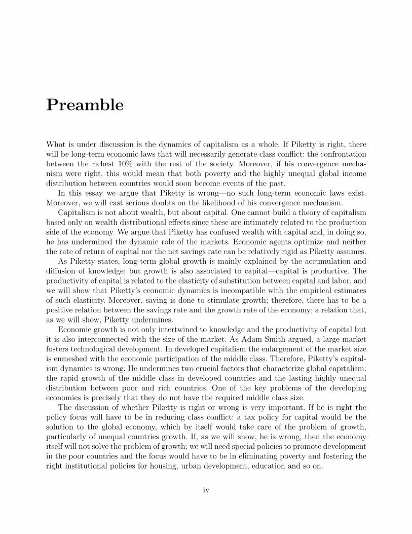
Preamble
What is under discussion is the dynamics of capitalism as a whole. If Piketty is right, therewill be long-term economic laws that will necessarily generate class conflict: the confrontationbetween the richest 10% with the rest of the society. Moreover, if his convergence mecha-nism were right, this would mean that both poverty and the highly unequal global incomedistribution between countries would soon become events of the past.
In this essay we argue that Piketty is wrong—no such long-term economic laws exist.Moreover, we will cast serious doubts on the likelihood of his convergence mechanism.
Capitalism is not about wealth, but about capital. One cannot build a theory of capitalismbased only on wealth distributional effects since these are intimately related to the productionside of the economy. We argue that Piketty has confused wealth with capital and, in doing so,he has undermined the dynamic role of the markets. Economic agents optimize and neitherthe rate of return of capital nor the net savings rate can be relatively rigid as Piketty assumes.
As Piketty states, long-term global growth is mainly explained by the accumulation anddiffusion of knowledge; but growth is also associated to capital—capital is productive. Theproductivity of capital is related to the elasticity of substitution between capital and labor, andwe will show that Piketty’s economic dynamics is incompatible with the empirical estimatesof such elasticity. Moreover, saving is done to stimulate growth; therefore, there has to be apositive relation between the savings rate and the growth rate of the economy; a relation that,as we will show, Piketty undermines.
Economic growth is not only intertwined to knowledge and the productivity of capital butit is also interconnected with the size of the market. As Adam Smith argued, a large marketfosters technological development. In developed capitalism the enlargement of the market sizeis enmeshed with the economic participation of the middle class. Therefore, Piketty’s capital-ism dynamics is wrong. He undermines two crucial factors that characterize global capitalism:the rapid growth of the middle class in developed countries and the lasting highly unequaldistribution between poor and rich countries. One of the key problems of the developingeconomies is precisely that they do not have the required middle class size.
The discussion of whether Piketty is right or wrong is very important. If he is right thepolicy focus will have to be in reducing class conflict: a tax policy for capital would be thesolution to the global economy, which by itself would take care of the problem of growth,particularly of unequal countries growth. If, as we will show, he is wrong, then the economyitself will not solve the problem of growth; we will need special policies to promote developmentin the poor countries and the focus would have to be in eliminating poverty and fostering theright institutional policies for housing, urban development, education and so on.
iv
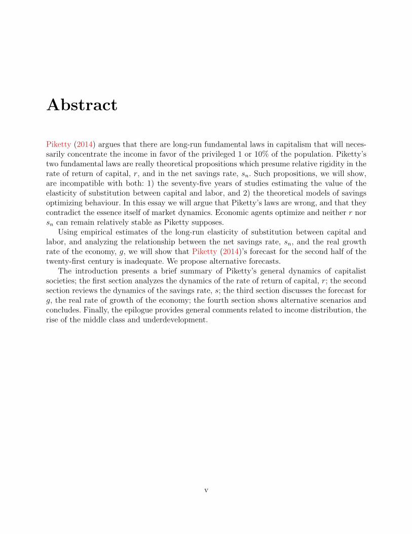
Abstract
Piketty (2014) argues that there are long-run fundamental laws in capitalism that will neces-sarily concentrate the income in favor of the privileged 1 or 10% of the population. Piketty’stwo fundamental laws are really theoretical propositions which presume relative rigidity in therate of return of capital, r, and in the net savings rate, sn. Such propositions, we will show,are incompatible with both: 1) the seventy-five years of studies estimating the value of theelasticity of substitution between capital and labor, and 2) the theoretical models of savingsoptimizing behaviour. In this essay we will argue that Piketty’s laws are wrong, and that theycontradict the essence itself of market dynamics. Economic agents optimize and neither r norsn can remain relatively stable as Piketty supposes.
Using empirical estimates of the long-run elasticity of substitution between capital andlabor, and analyzing the relationship between the net savings rate, sn, and the real growthrate of the economy, g, we will show that Piketty (2014)’s forecast for the second half of thetwenty-first century is inadequate. We propose alternative forecasts.
The introduction presents a brief summary of Piketty’s general dynamics of capitalistsocieties; the first section analyzes the dynamics of the rate of return of capital, r; the secondsection reviews the dynamics of the savings rate, s; the third section discusses the forecast forg, the real rate of growth of the economy; the fourth section shows alternative scenarios andconcludes. Finally, the epilogue provides general comments related to income distribution, therise of the middle class and underdevelopment.
v
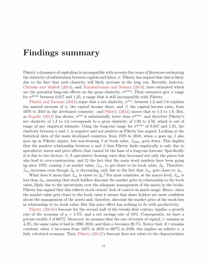
Findings summary
Piketty’s dynamics of capitalism is incompatible with seventy-five years of literature estimatingthe elasticity of substitution between capital and labor, σ. Piketty has argued that this is likelydue to the fact that such elasticity will likely increase in the long run. Recently, however,Chirinko and Mallick (2014), and, Karabarbounis and Neiman (2014), have estimated whichare the potential long-run effects on the gross elasticity, σgross. Their estimates give a rangefor σgross between 0.857 and 1.25, a range that is still incompatible with Piketty.
Piketty and Zucman (2014) argue that a net elasticity, σnet, between 1.2 and 1.6 explainsthe mutual increase of α, the capital income share, and β, the capital/income ratio, from1970 to 2010 in the developed countries—and Piketty (2014) moves that to 1.3 to 1.6. But,as Rognlie (2014) has shown, σnet is substantially lower than σgross, and therefore Piketty’snet elasticity of 1.2 to 1.6 corresponds to a gross elasticity of 1.93 to 2.56, which is out ofrange of any empirical estimate. Using the long-run range for σgross of 0.857 and 1.25, theelasticity between α and β, is negative and not positive as Piketty has argued. Looking at thehistorical data of the main developed countries, from 1970 to 2010, when α goes up β alsogoes up as Piketty argues, but non-housing β at book value, βnhbv, goes down. This impliesthat the positive relationship between α and β that Piketty finds empirically is only due tospeculative waves and price effects that cannot be the base of a long-run forecast. Specificallyit is due to two factors: 1) A speculative housing wave that increased not only the prices butalso lead to over-construction, and 2) the fact that the main stock markets have been goingup since 1970, causing β at market value, βmv, to get closer to its book value, βbv. Therefore,βmv increases even though βbv is decreasing, only due to the fact that βmv gets closer to βbv.
What does it mean that βmv is closer to βbv? For most countries, at the macro level, βmv isless than βbv, meaning that stock holders discount the market price in relationship to the bookvalue, likely due to the uncertainty over the adequate management of the assets in the books;Piketty has argued that this reflects stock owners’ lack of control on assets usage. Hence, whenthe market value gets closer to the book value it means that share holders are more confidentabout the management of the assets and, therefore, discount the market price of the stock lessin relationship to its book value. But this price effect has nothing to do with productivity.
Piketty (2014)’s forecast for the second half of the twenty-first century implies a growthrate of the economy of g = 1.5%, and a net savings rate of 10%. Consequently, we have aprivate wealth β of 667%. Moreover, he assumes that the rate of return of capital, r, remains in4.3%, the same value it had in 1990–2010, and then α becomes 28.7%. Notice that, if r remainsconstant, when β increases from 440% in 2010 to 667% in 2100, this implies an infinite σ, afully robotized economy. Then, Piketty (2014)’s forecast does not relate to the characteristics
vi
FINDINGS SUMMARY vii
of the production function in a productive capitalist economy—it does not relate to capital. Itis based upon short to medium term wealth sequels due to speculative waves and price effects.
Using Piketty’s forecasted β = 667% and σgross in the range of 0.857 to 1.25, we get anexaggerate downfall in α, in the wide range of 14.85% to 45.29% in relationship to the initialreference α. We also have a very low r, compared to historical statistics, in the range of 1.55%to 2.42%. Obviously something is wrong, either β or the range of σgross. Piketty argues thatthe historical data shows that the elasticity must be higher, but this argument is wrong sincethe historical positive co-movement between α and β is only due to the speculative housingwave and to the fact that βmv is getting closer to βbv. In the very long run the relationshipbetween βmv and βbv must be stable and the speculative housing wave must recede. Therefore,what must be wrong in the forecast has to be β. Since β is equal to the net savings ratedivided by the real growth rate of the economy, β = sn/g, then either sn or g are incorrectlyforecasted. If we assume that g is correctly forecasted, then sn must be off range.
Krusell and Smith (2015) showed, in models where the economic agents optimize, that boththe gross and the net savings rates are functions of g. They also showed that these modelsexplain well the American economy. But, given the available data for the world economy it isnot possible to calibrate these models. However, in a Solow model, with a given gross savingsrate, the net savings rate becomes a function of g. Hence, using empirical evidence of themain developed countries for the gross savings rate during 1991–2010, which fell in relation toprevious periods due to the fall of g, we have estimated the net savings rate corresponding to agrowth rate of the economy of 1.5% assumed by Piketty for the second half of the twenty-firstcentury. We have obtained a weighted average of sn = 6.40%, substantially lower than Piketty’s10%. Since Piketty’s overall assumption that g globally converges to that of the developedeconomies, this is a good estimate corresponding to a growth rate of 1.5%. With sn = 6.40%we have that β = 427% and using σgross in the range of 0.857 to 1.25, we obtain an r in therange of 4.47% to 4.55%, which is compatible with the historical evidence and with Piketty’sintuition that r should be around 4%. Since initially β was 440%, β = 427% represents a smalldownfall and produces modest increasing returns, therefore α actually increases. It must benoted that α increases when β falls and not when β goes up as Piketty has proposed. Moreover,α increases very modestly, in the range of 0.8% to 2.6% in relationship to its initial value.This implies that the capitalists will increase their income share between 0.16% and 0.5%;quite different from Piketty’s forecast which implied an increase of 9.75%.
We also estimate an alternative scenario with g growing at 2.1% instead of Piketty’s 1.5%.In this case sn = 8.07%, and β = 384%. The higher fall in β then triggers more significantincreasing returns and the estimated r goes up to the range of 5.1% to 5.47%. Consequently αincreases more aggressively but still in a moderate range of 3.65% to 11.10% above its initialreference value. This would imply that the capitalists’ income share would increase between0.69% and 2.1%, again much lower than Piketty’s forecasted 9.75%.
We conclude that there is not an invisible hand that will necessarily drive capitalismtowards income concentration in favor of the capitalists. Markets work and it is difficult toenvision that, only due to economic forces, the income distribution will worsen significantly;and in any case, if this happened, it would be due to capital scarcity and not due to capitalabundance as Piketty has suggested.
Introduction: Piketty’s capitalistsociety general dynamics
Piketty argues that the world economy will reduce its growth rate in the twenty-first centuryand that there are fundamental laws of capital accumulation that will necessarily lead to asubstantial increase in the capital/income ratio, β, as well as in the capital’s share of income,α; and because wealth is heavily concentrated, this will imply a considerable worsening of thepersonal income distribution, particularly in favor of the richest 1% or 10%. The consequence,is that the inheritance flow will increase, and a greater proportion of income will be derivedfrom rents on inherited wealth and less from income related to one’s own effort. Therefore, theprocess of capital accumulation threatens the core values of meritocratic societies. The naturalconsequences of the general laws of capital accumulation had been in the past ameliorated byexogenous shocks—such as the two wars and the policies adopted as a consequence—but thetendency will be reestablished in the twenty-first century. Therefore, argues this author, it isneeded that institutions adopt policies opposing such general tendency of capitalism, so heproposes a global tax on capital.
Piketty distinguishes forces pushing toward convergence and divergence. The principalconvergence mechanism, particularly related to the income distribution between countries, isthe diffusion of knowledge and the investment in training and skills. The main divergencemechanism is the process of capital accumulation itself. The divergence forces are of suchmagnitude that, if they are not opposed by adequate institutional policies, they will destroythe meritocratic society. There are also other proposals from Piketty such as the argument thatthe salaries of top american executives are better explained by power relationships and not bymarginal productivity. Through all his book there are interesting comments and discussionsabout several topics in economics. Some of them are of great relevance, like the need andconvenience to regulate and tax capital invested in fiscal paradises.
Piketty’s first conclusion is that “The history of the distribution of wealth has alwaysbeen deeply political, and it cannot be reduced to purely economic mechanisms”. His secondconclusion is that “. . . the dynamics of wealth distribution reveal powerful mechanisms pushingalternatively toward convergence and divergence”, Piketty (2014, p. 21). And “The crucial factis that no matter how potent a force, the diffusion of knowledge and skills may be, especially inpromoting convergence between countries, it can nevertheless be thwarted and overwhelmedby powerful forces pushing in the opposite direction, toward greater inequality”, Piketty (2014,p. 22). In summary, the divergence force of capital accumulation is more powerful than theconvergence force of diffusion of knowledge, but it can be opposed politically by institutional
viii
INTRODUCTION: PIKETTY’S CAPITALIST SOCIETY GENERAL DYNAMICS ix
policies; therefore what is needed is a political decision and Piketty proposes the global incometax—and understanding the complications of such tax he suggests to start with the EuropeanUnion.
This author uses both empirical and theoretical instruments. His empirical analysis cen-tres in developed countries but his general dynamics, he argues, is also applicable to under-developed countries and to the global mechanics of capitalism. Empirically, he constructs animpressive database of income and wealth in the main developed countries. Theoretically, heuses a neoclassical model of economic growth with peculiar characteristics that he introduces.Piketty reopens the question of the income distribution in capitalism. If anything, it becomesclearly established that the capitalist system does not necessarily solve the income distribu-tion problem. The income distribution depends crucially in the institutional arrangement onwhich the capitalist structure exists. Piketty’s three critical contributions are: 1) he reopensthe discussion on the topic of income distribution, 2) the creation of a relevant database which,despite requiring improvements, allows such discussion, and 3) his insistence that the incomedistribution amongst the factors of production is not necessarily stable.
But this author further pretends to unravel the fundamental dynamics of capitalism. Hisbook then inserts itself in the long tradition of classical economics, particularly the one ofRicardo and Marx. For Piketty, the dynamics of capitalism is given by what he calls thetwo fundamental laws of capitalism, which necessarily imply a social conflict amongst socialclasses, particularly between the richest 1% or 10% and the rest of society.
Chapter 1
Piketty’s Proposal
His proposal can be easily derived from his two fundamental laws of capitalism. The first lawis an accounting expression which necessarily holds at any point in time and it is expressedby
α = rβ. (1.1)
This expression tells us that the capital’s share of income, α, is equal to the product of therate of return on capital, r, and the capital/income ratio, β. The total income, Y , is equal tothe capital income, C, plus the labor income, L; therefore α = C
(C+L), and β = K
Y, where K is
the capital stock, whose usage produces the capital income C.The second law is an economic relationship which requires the passage of time (decades)
to realize itself. It is a condition of what is known as the stationary state, which is nothingelse than the equilibrium which the economy must necessarily reach in the long run. This lawaccording to Piketty comes from Harrod and Solow growth models but, as we will show, thereare crucial differences. This law is expressed by
β =s
g, (1.2)
which tells us that β, the capital/income ratio, is equal to the savings rate, s, divided bythe rate of growth of the economy, g. The savings rate, s, is equal to the total savings, S,divided by the total income Y . The rate of economic growth, g, is obtained by multiplyingthe population growth rate by the per capita income growth rate. Piketty presents all thevariables in net terms. Putting together (1.1) and (1.2) we obtain:
α
r= β =
s
g. (1.3)
Piketty’s capitalist accumulation process maintains relatively constant s and r. Therefore wheng falls, with s relatively constant, β goes up; and with r relatively constant, when β goes upα goes up. Therefore a fall on g, due to a fall either in the rate of growth of the populationor in the product per capita, implies that both the capital income/ratio, β, and the capital’sshare, α, go up. And with a wealth distribution favouring the high classes, understood as therichest 1% or 10%, the consequence of α going up is that the income of the high classes goesup in relationship to the rest of the society and the income distribution worsens.
1
CHAPTER 1. PIKETTY’S PROPOSAL 2
Note that (1.3) defines a stationary state, the necessary equilibrium to be reached in thelong run, which in the real world could imply decades. This expression is useful to understandwhat happens in the long run when g falls; which implies the motion of the economy fromone stationary state with a higher g to another one with lower g. A simple way to conceivea stationary state is to imagine an economy which saves 10% of income, produces an incomeof 100 and grows annually at 2%; the question is: Which should be the value of β in thisstationary state? Since a stationary state implies that the value of β must be permanent, βmust grow at the same rate as income, at 2%. If savings are 10 and they are equal to 2%, thenthe capital stock necessarily must be equal to 500, and β is equal to 5.
Piketty’s forecast for the second half of the twenty-first century is based on the previouslydescribed process. He assumes that g falls to 1.5% and, with s relatively stable at 10%, βwill be, in the stationary state, equal to 667%. And with r relatively stable in 4.3%; α willbe 29% and the the labor income share equals 71%. The increase in α, given a pronouncedwealth ownership concentration, implies an income concentration in favor of the richest 1%or 10%. Finally, the greater the income of the high classes, the higher the inheritance flows;this tendency is strengthened due to the fact that a lower demographic growth implies lessdescendants per family and a higher inheritance per each one. A higher inheritance flow impliesthe rapid growth of the renter’s class and threatens the basic values of the developed societies,which consider themselves meritocracies.
In the previously described process there are three key variables whose behaviour definesPiketty’s forecast: the fall in g and the relative stability of s and r. In particular, with s and rrelatively stable, the concentration of income and the increase in the inheritance flow will behigher the lower g falls in relationship to r. The process depends crucially on r−g. The higher rin relationship to g, the more pronounced the high class’ accumulative capacity in relationshipto the rest of the economy. For Piketty, institutions must preclude the consequences that heheralds, thus as α goes up they must introduce a global tax on capital; since finally whatcounts for the income distribution is the r after taxes. One of the benefits of the global taxwould be to finish with the anonymity of the capital that flies to fiscal paradises, anotherbenefit is to gain transparency on inheritance and income distribution statistics.
In what follows we will focus on the dynamics of the three key variables in the process:the rate of return to capital r, the savings rate s, and the rate of growth of the economy g.Such dynamics will be analyzed both theoretically and empirically.
Chapter 2
The dynamics of r
The rate of return of capital, r, is measured empirically in national accounts. It is the ex postrealized r. This historical r is given by economic influences as well as by institutional factors.Economically this r has two main contradictory influences, on the one hand there is the law ofdecreasing returns which says that when capital increases, r must fall; on the other hand thereis technological development which shifts the production function and which can allow r toremain high, or even to increase when capital goes up. Observe however that the technologyof relevance is only that which is capital-incorporated. Institutionally r is the consequenceof power relations which manifest themselves in specific policies, for example in the twenty-first century there are two tendencies: the statist policies consequence of the two wars andthe neoliberal policies which start in the 80s. Independently of tax raises or reductions, thesalary policy, for example, is critical. Economically if r stays high, when β goes up, it meansthat the capital-incorporated technological development is more powerful than the decreasingreturns. Politically r can be defined by the relative power of the social classes. In particular,in an autocratic society, the rent is not necessarily due to market conditions; and even indemocratic societies, the relative power of the social classes can influence r in a significantway.
In economic theory the discussion around the dynamics of r centres in the relative strengthof the diminishing returns versus technological development. If we maintain s relatively con-stant, then in (1.3) when g goes down β goes up, and then if α goes up or not will dependon whether r remains relatively constant or not. But what does it mean that r remains highenough, despite β increases, so that r − g remains also elevated? It means that capital, inspite of its increased size, remains productive. It means that the elasticity between capitaland labor, σ, is high. Conceptually in a constant elasticity of substitution production func-tion, this means that σ is greater than one. Since the elasticity between α and β, σαβ, is givenby 1 − 1/σ, in general if σ > 1, σαβ will be positive. Which means that if β goes up, α alsogoes up. Note that if σ goes to infinity, it means that capital is a perfect substitute of labor, afully robotized economy. Piketty and Zucman (2014) infer that, given the fact that empiricallyfrom 1970 to 2010 both β and α go up, then σ > 1; they estimate σ in the range of 1.2 to1.6—Piketty (2014) changes the range to 1.3 to 1.6. But such inference has been challengedby Rognlie (2014).
3
CHAPTER 2. THE DYNAMICS OF r 4
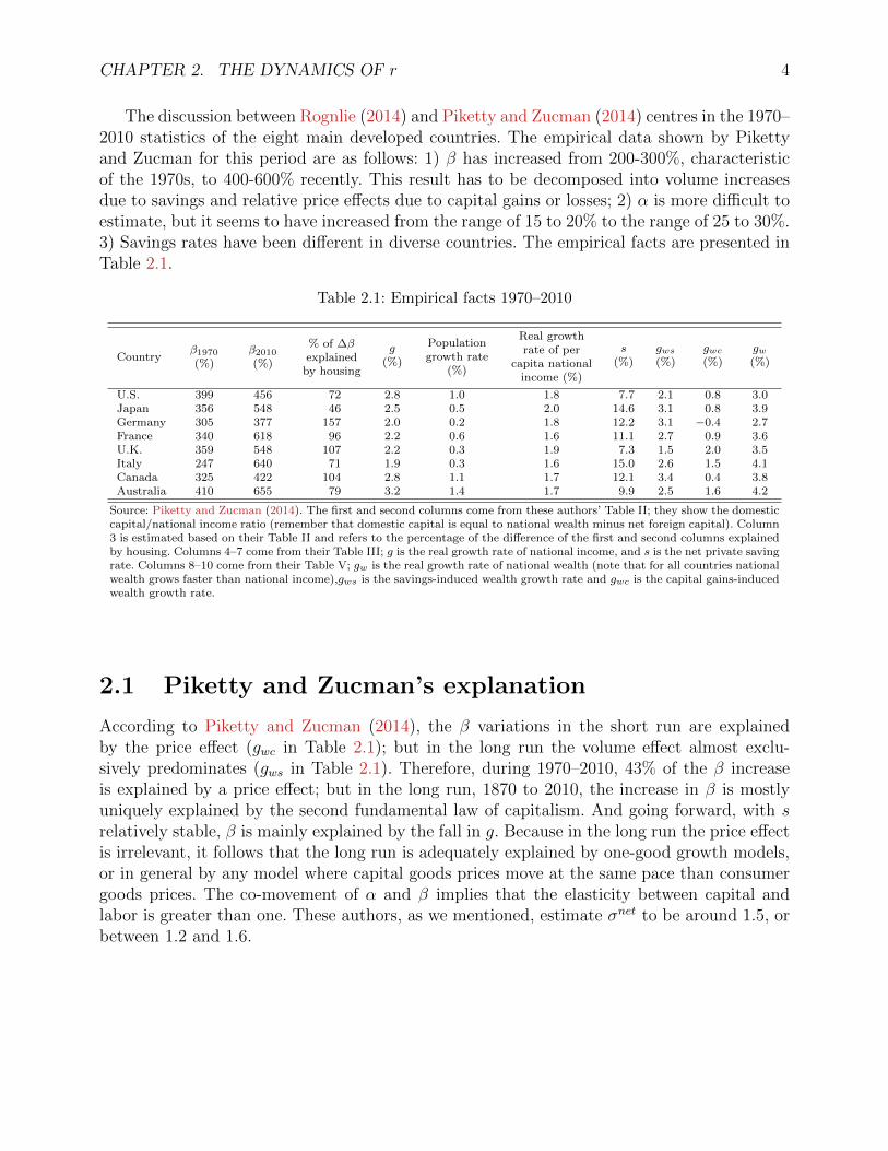
The discussion between Rognlie (2014) and Piketty and Zucman (2014) centres in the 1970–2010 statistics of the eight main developed countries. The empirical data shown by Pikettyand Zucman for this period are as follows: 1) β has increased from 200-300%, characteristicof the 1970s, to 400-600% recently. This result has to be decomposed into volume increasesdue to savings and relative price effects due to capital gains or losses; 2) α is more difficult toestimate, but it seems to have increased from the range of 15 to 20% to the range of 25 to 30%.3) Savings rates have been different in diverse countries. The empirical facts are presented inTable 2.1.
Table 2.1: Empirical facts 1970–2010
Countryβ1970(%)
β2010(%)
% of ∆βexplained
by housing
g(%)
Populationgrowth rate
(%)
Real growthrate of per
capita nationalincome (%)
s(%)
gws(%)
gwc(%)
gw(%)
U.S. 399 456 72 2.8 1.0 1.8 7.7 2.1 0.8 3.0Japan 356 548 46 2.5 0.5 2.0 14.6 3.1 0.8 3.9Germany 305 377 157 2.0 0.2 1.8 12.2 3.1 −0.4 2.7France 340 618 96 2.2 0.6 1.6 11.1 2.7 0.9 3.6U.K. 359 548 107 2.2 0.3 1.9 7.3 1.5 2.0 3.5Italy 247 640 71 1.9 0.3 1.6 15.0 2.6 1.5 4.1Canada 325 422 104 2.8 1.1 1.7 12.1 3.4 0.4 3.8Australia 410 655 79 3.2 1.4 1.7 9.9 2.5 1.6 4.2
Source: Piketty and Zucman (2014). The first and second columns come from these authors’ Table II; they show the domesticcapital/national income ratio (remember that domestic capital is equal to national wealth minus net foreign capital). Column3 is estimated based on their Table II and refers to the percentage of the difference of the first and second columns explainedby housing. Columns 4–7 come from their Table III; g is the real growth rate of national income, and s is the net private savingrate. Columns 8–10 come from their Table V; gw is the real growth rate of national wealth (note that for all countries nationalwealth grows faster than national income),gws is the savings-induced wealth growth rate and gwc is the capital gains-inducedwealth growth rate.
2.1 Piketty and Zucman’s explanation
According to Piketty and Zucman (2014), the β variations in the short run are explainedby the price effect (gwc in Table 2.1); but in the long run the volume effect almost exclu-sively predominates (gws in Table 2.1). Therefore, during 1970–2010, 43% of the β increaseis explained by a price effect; but in the long run, 1870 to 2010, the increase in β is mostlyuniquely explained by the second fundamental law of capitalism. And going forward, with srelatively stable, β is mainly explained by the fall in g. Because in the long run the price effectis irrelevant, it follows that the long run is adequately explained by one-good growth models,or in general by any model where capital goods prices move at the same pace than consumergoods prices. The co-movement of α and β implies that the elasticity between capital andlabor is greater than one. These authors, as we mentioned, estimate σnet to be around 1.5, orbetween 1.2 and 1.6.
CHAPTER 2. THE DYNAMICS OF r 5
2.2 The Problems with Piketty and Zucman’s explana-
tion
Solow (2014), in his very positive comment on Piketty (2014), mentions that there is certainlevel of confusion between the definitions of capital and wealth; but he does not go deeper,and, as we will argue, he should have done so, because this seems to be the main problem withPikkety and Zucman’s explanation. The problem resides in the fact that for them wealth andcapital are identical. Piketty defines capital “as the total market value of everything ownedby the residents and government of a given country at a given point in time, provided thatit can be traded on some market” (see Piketty, 2014, p. 48). Therefore, national wealth =national capital = domestic capital + net foreign capital. Capital does not include humancapital, but it does include physical capital such as: land, housing, buildings, infrastructure,equipment and other forms of physical capital; and also immaterial capital such as patents andintellectual property. The capital income, C, and the rate of return of capital, r, then include“rents, profits, dividends, interest, royalties, etc., excluding interest on public debt (rememberthese are both an asset and a liability, therefore at the national level they wash out), beforetaxes” (2014, pp. 201-203; italics added).
In economic theory, capital is an input of production subject to the law of diminishingreturns, and it is everything in the production function which is not labor. The fundamentalcharacteristic of capital is that it is used to produce. Capital is about quantities, not prices.Therefore, any attempt to measure capital must take away price effects. Housing is one of theways to accumulate wealth, and since houses are needed in a productive economy, housingmust also be considered to a large extent as capital. But there is a fine distinction to be madeas to which proportion of saving in housing is really capital and which is not. Because of itspeculiar characteristics, it is necessary to analyze housing independently of the rest of capital.In particular the price of housing incorporates the price of the land on which it stands. Andland is clearly different to the rest of capital. It is not reproducible and as a consequence itcan present relative scarcities, which could increase its real price. Land does not depreciate,it appreciates. But lets look specifically why Piketty’s definition of capital is problematic forthe interpretation he makes of the data he presents.
2.3 The discussion about capital gains and the rise in
the price of land
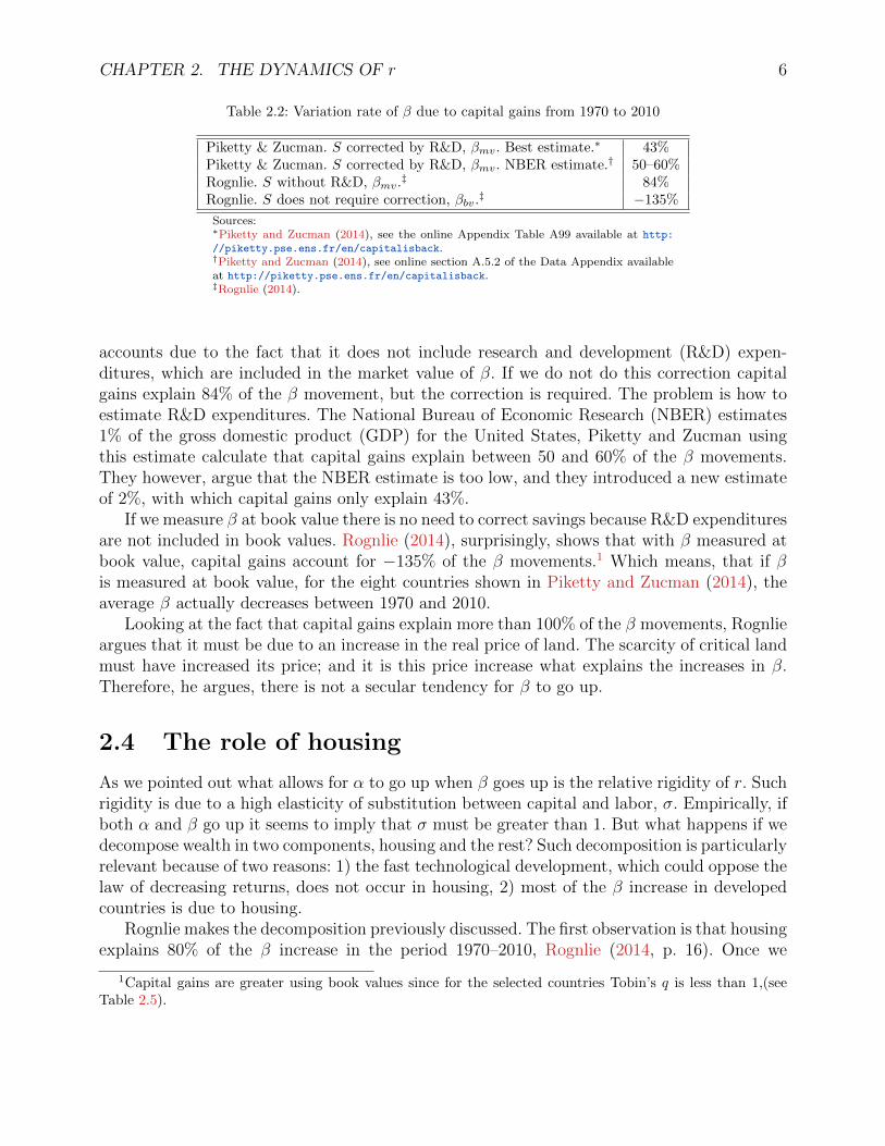
As we previously mentioned capital is about quantities, hence we need to remove price effects.Piketty and Zucman do it by differentiating volume effects due to savings from capital gainsor losses. In this context, it becomes critical how much of the β increase is only due to priceeffects. The discussion is how to measure capital gains; and it is related as to how to bettermeasure β, if at market prices or at book value. The results are quite different. Table 2.2shows the outcome. If β is measured at market value, βmv, capital gains explain between 43%and 55% of the β increase; if β is measured at book value, βbv, capital gains explain −135%.
If we measure β at market values we must correct savings, S, as it appears in national
CHAPTER 2. THE DYNAMICS OF r 6
Table 2.2: Variation rate of β due to capital gains from 1970 to 2010
Piketty & Zucman. S corrected by R&D, βmv. Best estimate.∗ 43%Piketty & Zucman. S corrected by R&D, βmv. NBER estimate.† 50–60%Rognlie. S without R&D, βmv.
‡ 84%Rognlie. S does not require correction, βbv.
‡ −135%
Sources:∗Piketty and Zucman (2014), see the online Appendix Table A99 available at http:
//piketty.pse.ens.fr/en/capitalisback.†Piketty and Zucman (2014), see online section A.5.2 of the Data Appendix availableat http://piketty.pse.ens.fr/en/capitalisback.‡Rognlie (2014).
accounts due to the fact that it does not include research and development (R&D) expen-ditures, which are included in the market value of β. If we do not do this correction capitalgains explain 84% of the β movement, but the correction is required. The problem is how toestimate R&D expenditures. The National Bureau of Economic Research (NBER) estimates1% of the gross domestic product (GDP) for the United States, Piketty and Zucman usingthis estimate calculate that capital gains explain between 50 and 60% of the β movements.They however, argue that the NBER estimate is too low, and they introduced a new estimateof 2%, with which capital gains only explain 43%.
If we measure β at book value there is no need to correct savings because R&D expendituresare not included in book values. Rognlie (2014), surprisingly, shows that with β measured atbook value, capital gains account for −135% of the β movements.1 Which means, that if βis measured at book value, for the eight countries shown in Piketty and Zucman (2014), theaverage β actually decreases between 1970 and 2010.
Looking at the fact that capital gains explain more than 100% of the β movements, Rognlieargues that it must be due to an increase in the real price of land. The scarcity of critical landmust have increased its price; and it is this price increase what explains the increases in β.Therefore, he argues, there is not a secular tendency for β to go up.
2.4 The role of housing
As we pointed out what allows for α to go up when β goes up is the relative rigidity of r. Suchrigidity is due to a high elasticity of substitution between capital and labor, σ. Empirically, ifboth α and β go up it seems to imply that σ must be greater than 1. But what happens if wedecompose wealth in two components, housing and the rest? Such decomposition is particularlyrelevant because of two reasons: 1) the fast technological development, which could oppose thelaw of decreasing returns, does not occur in housing, 2) most of the β increase in developedcountries is due to housing.
Rognlie makes the decomposition previously discussed. The first observation is that housingexplains 80% of the β increase in the period 1970–2010, Rognlie (2014, p. 16). Once we
1Capital gains are greater using book values since for the selected countries Tobin’s q is less than 1,(seeTable 2.5).
CHAPTER 2. THE DYNAMICS OF r 7
eliminate housing, he estimates, there is only a small increase in β and a small decreasein α, which means σ < 1, and a lower r. Why when we include housing σ is greater thanone, and when we exclude it σ is less than one? The basic reason argued by Rognlie, as wementioned before, is that the real price of land has risen, and therefore the one-good modelused by Piketty and Zucman becomes inadequate. When the price of land goes up, becauseits consumption is inelastic, the proportion of income spent in housing goes up, and this is themain cause of the observed increases in β. To estimate σ from the co-movement of α and β isnot possible whenever the real price of capital moves differently than the price of consumptiongoods—the case of land. Rognlie has argued that the co-movement observed between α andβ, during 1970–2010, is due to the increase in the price of land; that is why, he says, that abetter title for Piketty’s book would have been Housing in the Twenty-First Century.
Rognlie shows that if g falls, for example from 3% to 1.5%, r − g falls rapidly. Only if wewere out of Piketty’s world, with s being a positive function of g, it would be possible thatwhen g falls, as s also falls, r− g could remain high. But in such a world β would go up muchless than what Piketty assumes—see the next section about the dynamics of savings.
The discussion between Rognlie and Piketty-Zucman has great relevance, because if thesecular tendency of β to increase cannot be shown for 1970–2010, which is the period forwhich we have solid national accounts, Pikkety’s explanation of the dynamics of capitalism isin trouble.
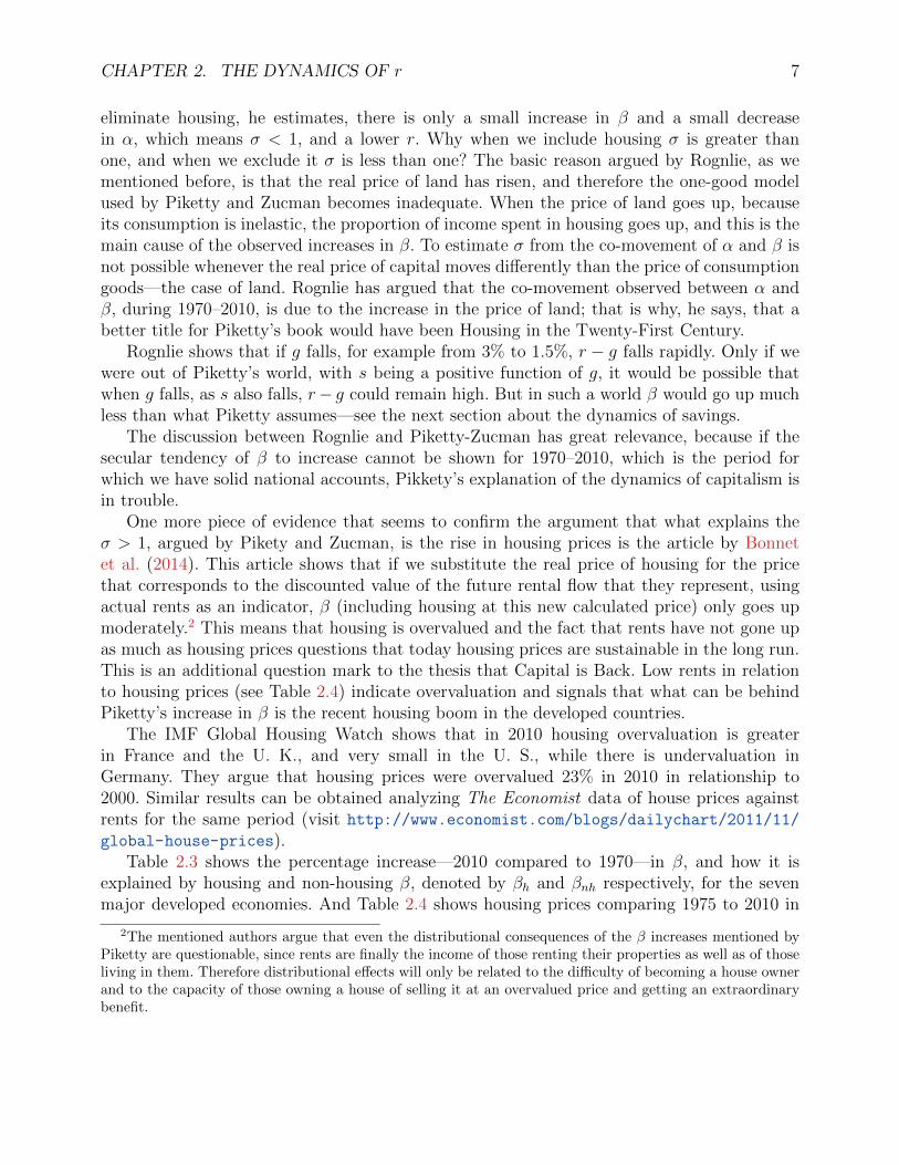
One more piece of evidence that seems to confirm the argument that what explains theσ > 1, argued by Pikety and Zucman, is the rise in housing prices is the article by Bonnetet al. (2014). This article shows that if we substitute the real price of housing for the pricethat corresponds to the discounted value of the future rental flow that they represent, usingactual rents as an indicator, β (including housing at this new calculated price) only goes upmoderately.2 This means that housing is overvalued and the fact that rents have not gone upas much as housing prices questions that today housing prices are sustainable in the long run.This is an additional question mark to the thesis that Capital is Back. Low rents in relationto housing prices (see Table 2.4) indicate overvaluation and signals that what can be behindPiketty’s increase in β is the recent housing boom in the developed countries.
The IMF Global Housing Watch shows that in 2010 housing overvaluation is greaterin France and the U. K., and very small in the U. S., while there is undervaluation inGermany. They argue that housing prices were overvalued 23% in 2010 in relationship to2000. Similar results can be obtained analyzing The Economist data of house prices againstrents for the same period (visit http://www.economist.com/blogs/dailychart/2011/11/
global-house-prices).Table 2.3 shows the percentage increase—2010 compared to 1970—in β, and how it is
explained by housing and non-housing β, denoted by βh and βnh respectively, for the sevenmajor developed economies. And Table 2.4 shows housing prices comparing 1975 to 2010 in
2The mentioned authors argue that even the distributional consequences of the β increases mentioned byPiketty are questionable, since rents are finally the income of those renting their properties as well as of thoseliving in them. Therefore distributional effects will only be related to the difficulty of becoming a house ownerand to the capacity of those owning a house of selling it at an overvalued price and getting an extraordinarybenefit.
CHAPTER 2. THE DYNAMICS OF r 8
real terms as well as against rents and against average income. In France and the UnitedKingdom, where houses are significantly overvalued, the percentage increase in total β wasvery high and it is more than totally explained by housing. In Australia and Canada housesare also significantly overvalued and the % total β increase is as high or higher than in theU.K.; in Australia almost all of the percentage increase in β is explained by housing, while inCanada a portion of the increase is due to βnh.
In the U.S., where houses are close to their value, housing also explains more than thepercentage increase in total β, but the β increase was very moderate. In Germany housing isundervalued, therefore the percentage increase in total β, which is more than fully explainedby housing, represents real savings related to the reconstruction of East Germany. This re-construction of East Germany will later on explain, in Table 3.2, why savings remain high forGermany despite the fall in the rate of growth of the economy. In Japan most of the total βincrease is due to non-housing and the part due to housing is also related to real savings be-cause houses are undervalued. These two facts will explain later on, in Table 2.5, why Japanis the only country where there is an inverse relationship between α increases and total βincreases at market value.
Table 2.3: Percentage increase in β explained by βh and βnh from 1970 to 2010
U.S. U.K. France Germany Japan Canada Australiaβ increase (%) 7 45 73 33 71 45 50Explained by βh (%) 10 55 76 34 25 35 49Explained by βnh (%) −3 −10 −3 −1 46 10 1
Source: Author’s calculations based on Appendix Tables A1 and A16 of Piketty and Zucman (2014), availableat http://piketty.pse.ens.fr/en/capitalisback. The increase explained by βnh is calculated based on thesetables.
Table 2.4: Housing prices 1975–2010
U.S. U.K. France Germany Japan Canada AustraliaIn real terms∗ 120.9 205.2 230.5 85.5 89.9 211.8 279.1Against rents† 96.4 137.2 137.0 76.9 66.6 158.3 157.8Against average income† 84.3 118.9 130.5 75.6 68.8 125.1 133.3
Source: The Economist house-price index available at http://www.economist.com/blogs/dailychart/2011/11/global-house-prices.∗Q4 2010 vs. Q1 1975 (= 100).†Q4 2010 vs Long-term average (= 100).
2.5 Price effects and speculative waves
Capital must be productive and it includes housing when it is productive. But housing does notbehave like the rest of capital, it can have long speculative waves which will not only overvaluehousing—which will show in capital gains—but also will produce over-construction—which
CHAPTER 2. THE DYNAMICS OF r 9
will be reflected in more savings. Both components will increase βh and the total β. Theselong waves will increase wealth and may have repercussions in the capital income share, α.But such waves cannot be the base of a long-run forecast, because the high prices and theover-construction will have an end as they build the forces of their own destruction. Thus,while housing can influence the growth of β in the medium term, it will not be a decisivefactor in the long run.
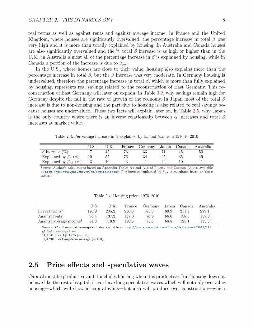
Moreover, speculative housing waves are not unique in influencing β in the medium term,there are other effects which need to be discussed; amongst them, the relationship between βbvand βmv. Looking at the historical data of the main developed countries we find that from 1970to 2010 when α goes up market value national wealth-national income ratio, βmv, also goesup as Piketty argues; but β at book value, βbv, goes down both in the U.S. and in the U.K.(See Table 2.5). This implies that in these countries the positive relationship between α andβ that Piketty finds is partially due to the fact that the main stock markets have been goingup since 1970, which has occationed that βmv get closer to βbv; in other words the Tobin’s qratios have been going up. They have been going up particularly in the U.S. and the U.K.(see Table 2.5). Therefore, βmv increases, despite the fact that βbv is decreasing, only due tothe fact that βmv gets closer to βbv.
What does it mean that βmv gets closer to βbv? When the market value gets closer tothe book value, or even exceeds it, it means that share holders are more confident as to themanagerial usage of assets and therefore stock owners discount the market price less in rela-tionship to its book value. But this process has nothing to do with productivity. The physicaland intellectual company capital does not go up when βmv gets closer to βbv; companies arethe same, we have only a price effect as stock owners decide to value more the stocks. Thisprice effect again cannot be the base of a long run forecast, because it has its own limits as tohow far it can go. In order to avoid the medium-term noise produced by this price effect, andto better describe the long-term relation between α and β, it is better to compare α, with βbv.
There is a long discussion in economics regarding the usefulness of βmv vs. βbv. There isno doubt that measuring capital at market prices has many advantages. Market prices takeinto account not only a view of the future through the discount rate used to value futureincome, but they also take into account present information in many variables—for exampleproven oil reserves. And market prices also include adequately intangible assets like researchand development. For the previous reasons book value is not a good substitute for marketvalue. However, market value is neither a good substitute of book value. They just providedifferent information, and both are useful. Market value has the problem that asset marketsare very volatile. Book value presents a better view of the quantity of inputs in a productionfunction; it allows us to take away the price effects.
In a stationary state there cannot be differences between the two measures, because ina stationary state there is no uncertainty about the future. This is the reason that we canestimate the stationary value of β given data on the growth rate of income and on the savingsrate. If some of the capital became unproductive then the value of β couldn’t be definedbecause it would not be permanent any longer. An stationary state means a repetitive economy,therefore it would make no sense in such an economy to book assets unless they are productive.Book values and market values must be aligned in the very long run because otherwise, why to
CHAPTER 2. THE DYNAMICS OF r 10
book assets that will not become productive? The trial and error and the constant innovationin real markets, doesn’t take away the fact that economic agents optimize and therefore willonly book those assets that they believe will be productive. Basic theory tells us that in thevery long run book values and market values must be aligned. In fact this is the very meaningof a stationary state.
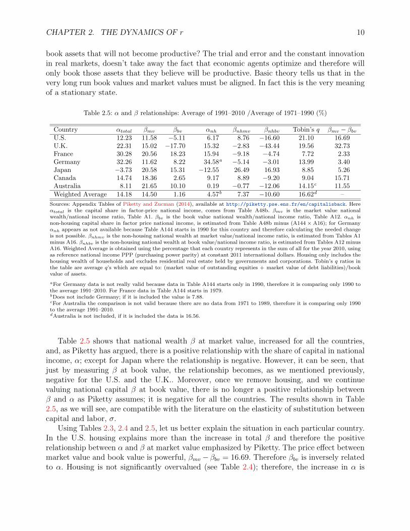
Table 2.5: α and β relationships: Average of 1991–2010 /Average of 1971–1990 (%)
Country αtotal βmv βbv αnh βnhmv βnhbv Tobin’s q βmv − βbvU.S. 12.23 11.58 −5.11 6.17 8.76 −16.60 21.10 16.69U.K. 22.31 15.02 −17.70 15.32 −2.83 −43.44 19.56 32.73France 30.28 20.56 18.23 15.94 −9.18 −4.74 7.72 2.33Germany 32.26 11.62 8.22 34.58a −5.14 −3.01 13.99 3.40Japan −3.73 20.58 15.31 −12.55 26.49 16.93 8.85 5.26Canada 14.74 18.36 2.65 9.17 8.89 −9.20 9.04 15.71Australia 8.11 21.65 10.10 0.19 −0.77 −12.06 14.15c 11.55Weighted Average 14.18 14.50 1.16 4.57b 7.37 −10.60 16.62d –
Sources: Appendix Tables of Piketty and Zucman (2014), available at http://piketty.pse.ens.fr/en/capitalisback. Hereαtotal is the capital share in factor-price national income, comes from Table A48b. βmv is the market value nationalwealth/national income ratio, Table A1. βbv is the book value national wealth/national income ratio, Table A12. αnh isnon-housing capital share in factor price national income, is estimated from Table A48b minus (A144 × A16); for Germanyαnh appears as not available because Table A144 starts in 1990 for this country and therefore calculating the needed changeis not possible. βnhmv is the non-housing national wealth at market value/national income ratio, is estimated from Tables A1minus A16. βnhbv is the non-housing national wealth at book value/national income ratio, is estimated from Tables A12 minusA16. Weighted Average is obtained using the percentage that each country represents in the sum of all for the year 2010, usingas reference national income PPP (purchasing power parity) at constant 2011 international dollars. Housing only includes thehousing wealth of households and excludes residential real estate held by governments and corporations. Tobin’s q ratios inthe table are average q’s which are equal to: (market value of outstanding equities + market value of debt liabilities)/bookvalue of assets.
aFor Germany data is not really valid because data in Table A144 starts only in 1990, therefore it is comparing only 1990 tothe average 1991–2010. For France data in Table A144 starts in 1979.bDoes not include Germany; if it is included the value is 7.88.cFor Australia the comparison is not valid because there are no data from 1971 to 1989, therefore it is comparing only 1990to the average 1991–2010.dAustralia is not included, if it is included the data is 16.56.
Table 2.5 shows that national wealth β at market value, increased for all the countries,and, as Piketty has argued, there is a positive relationship with the share of capital in nationalincome, α; except for Japan where the relationship is negative. However, it can be seen, thatjust by measuring β at book value, the relationship becomes, as we mentioned previously,negative for the U.S. and the U.K.. Moreover, once we remove housing, and we continuevaluing national capital β at book value, there is no longer a positive relationship betweenβ and α as Piketty assumes; it is negative for all the countries. The results shown in Table2.5, as we will see, are compatible with the literature on the elasticity of substitution betweencapital and labor, σ.
Using Tables 2.3, 2.4 and 2.5, let us better explain the situation in each particular country.In the U.S. housing explains more than the increase in total β and therefore the positiverelationship between α and β at market value emphasized by Piketty. The price effect betweenmarket value and book value is powerful, βmv − βbv = 16.69. Therefore βbv is inversely relatedto α. Housing is not significantly overvalued (see Table 2.4); therefore, the increase in α is
CHAPTER 2. THE DYNAMICS OF r 11
mostly due to real housing wealth, which may reflect some speculative over-construction, butthe percentage increase in total β is small. In principle since the % explained by βnh is negativein Table 2.3, one would expect βnhmv in Table 2.5 to go down, but it actually increases—thisis due to the additional effect of the stocks market value getting closer to their book value.As we can see the Tobin’s q average between the two periods increases the most in the U.S.(see Table 2.5), and, as we mentioned, what is even more significant, βmv − βbv is very high.But if we remove this price effect we find that βnhbv is inversely related to both αtotal and αnh(see Table 2.5).
In the U.K., again housing explains more than the β increase and therefore the positiverelation between α and βmv. In the U.K. the price effect between market values and book valuesis the strongest, βmv − βbv = 32.73. Therefore βbv is powerfully inversely related to α. Likethe U.S., the increase in β is very well explained by housing, but since houses are significantlyovervalued the increase in β is substantial (see Table 2.3). The percentage explained by non-housing in the U.K. is actually the most negative, therefore one would expect for βnh at marketvalue to go down and it actually does, but not by much because it is also influenced by thevery powerful price effect between market values and book values. The U.K. also has a verysignificant increase in Tobin’s q, and it has the highest difference between βmv and βbv whichshows the very powerful price effect mentioned. Once this price effect is removed and we valuenon-housing β at book value then the decrease is notoriously high. βnhbv is inversely related,like in all the countries, both to αtotal and to αnh.
In France again βh explains more than 100% of the β increase and therefore the positiverelation between α and βmv. In France houses are the most overvalued and the β increaseis also the highest. And like in the U.S. and the U.K., the total percentage increase of βexplained by βnh is negative therefore one should expect βnhmv to go down, and it actuallydoes significantly because the price effect between market values and book values is very smallin France, βmv − βbv is only 2.33. Again βnhbv is inversely related to α and to αnh.
In Germany housing explains again more than the total β increase, and therefore thepositive relation between α and β. But houses are undervalued, therefore the total β increaseis substantially lower than in all the other countries except the U.S.. Housing in Germany isrelated to real housing construction due to the reconstruction of East Germany. Again thepercentage explained by non-housing is negative, therefore one would expect βnh to go down,and it does because the price effect in Germany related to market value vs. book value issmall, βmv − βbv = 3.40. βnhbv again is inversely related to αtotal and to αnh.
In Japan housing only explains partially the total β increase, which is mostly explained bynon-housing β. Also the price effect related to market value vs. book value is small, Japan has alow Tobin’s q and a βmv − βbv equal only to 5.62. Moreover, housing in Japan is undervalued.Therefore, diminishing returns related to the significant increase in total β prevail in thewhole wealth and there is an inverse relationship between α and βmv. There is of course alsoan inverse relationship between all the other measures of β (βbv, βnhmv and βnhbv) and the twomeasures of capital income share, αtotal and αnh. Japan actually exemplifies what happens toan economy when the speculative housing wave is over and in which housing increases aredue to real construction, and where the price effefts between βmv and βbv are small, as theorywould suggest, the relationship between βmv and α is negative due to the diminishing returns
CHAPTER 2. THE DYNAMICS OF r 12
that predominate in all the wealth.In Canada housing is significantly overvalued and the total β increase is explained mostly
by housing, which explains the positive relationship between βmv and α. But the percentageexplained by non-housing is positive and significant, therefore one would expect for βnhmv togo up and it does, partially due to this effect and the high effect of market values vs. bookvalues, βmv − βbv = 15.71. But once we remove the price effect βnhbv will inversely relate, likein all cases to α and to αnh.
Finally, in Australia housing is the most overvalued and it explains almost all of the βincrease and the positive relation between βmv and α. Once we remove housing, βnhmv goesdown but only minimally because there’s is a significant price effect, βmv − βbv = 11.55. Oncewe remove the price effect βnhbv goes down and is inversely related to both α and αnh.
In summary: the positive relationship between α and βmv is due to housing and priceeffects between market value and book value wealth. If we remove the price effects, both theU.S. and the U.K. show a negative relationship between α and βbv. If we remove housing theU.K., France, Germany and Australia show an inverse relationship between βnhmv and α. Ifwe remove both housing and the price effects all the contries show an inverse relation betweenβnhbv and both α and αnh.
2.6 The elasticity between capital and labor
Everything seems to indicate that the gross elasticity of substitution between capital andlabor, σ (previously denoted as σgross), is less than 1.25. Chirinko and Mallick (2014) makea review on the literature estimating σ concluding that the best range estimate is 0.40–0.60.It is worth mentioning that the highest σ, found in aggregate investment data, is 1.59 andcorresponds to computers; and that the equipment σ, in panel data, is 0.93. Mallick (2007)estimates worldwide σ in 0.338, see also Mallick (2012). This author corroborates the de laGrandville hypothesis, and shows that there is a positive correlation between g and σ. Butanyway the highest σ which corresponds to East Asia is only 0.737. Chirinko and Mallick(2014) conclude that their best estimate is 0.406. They also estimate σ for heterogeneousindustries and amongst their results we find agriculture σ = 0.289, construction σ = 0.41,machinery σ = 0.483, electrical machinery σ = 0.486. The highest σ corresponds to finance,insurance and real estate and it is of 1.16. These authors analyze the possibility that σ mayrise in the future as economies develop, and they concentrate on a specific subset of industriesthat they call the post-industrial economy. But even if this were to happen the σ correspondingto the mentioned specific subset of industries is only 0.857. Oberfield and Raval (2014) arguethat even taking into account increases due to cross sector elasticity, the manufacturing sectorσ in the United States would not be higher than 0.7; and for the manufacturing sectors ofsome other countries the corresponding value will be σ = 0.84 for Chile and Colombia, andσ = 1.11 for India. Few authors in the past, who represent a minority, have argued that in thelong run σ = 1, see Jones (2005). And finally Karabarbounis and Neiman (2014) focus in long-term sequences, variation amongst sectors and use many industries and countries estimatingσ = 1.25. In summary, taking into account Piketty’s argument that σ may rise in the long run,one could expect for σ to be higher than the 0.406 estimated by Chirinko and Mallick (2014);
CHAPTER 2. THE DYNAMICS OF r 13
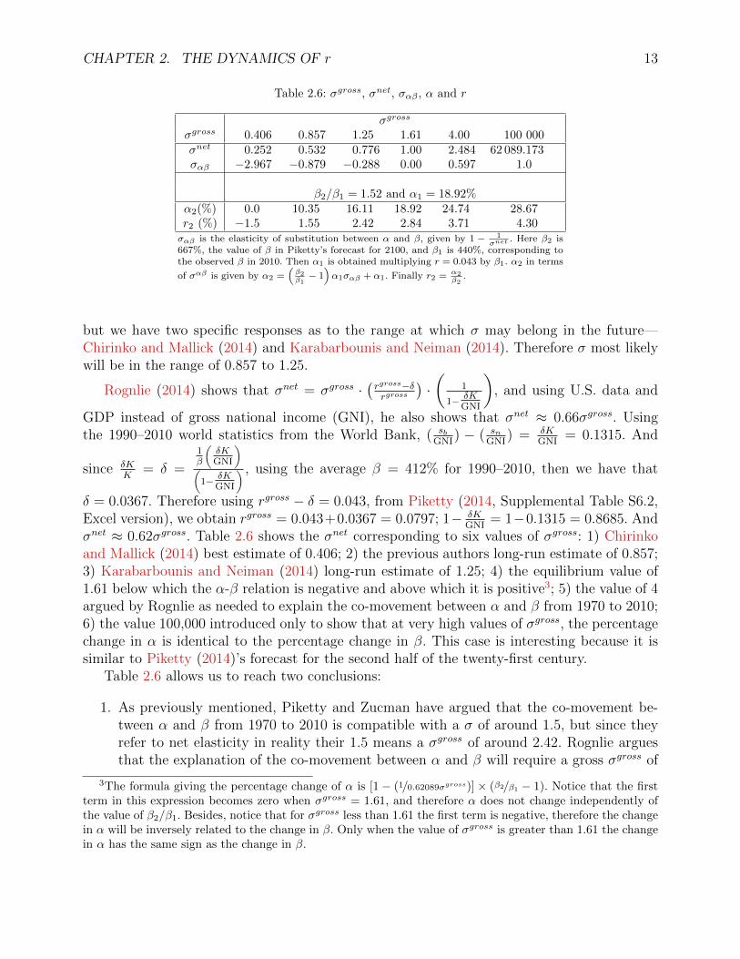
Table 2.6: σgross, σnet, σαβ , α and r
σgross
σgross 0.406 0.857 1.25 1.61 4.00 100 000σnet 0.252 0.532 0.776 1.00 2.484 62 089.173σαβ −2.967 −0.879 −0.288 0.00 0.597 1.0
β2/β1 = 1.52 and α1 = 18.92%α2(%) 0.0 10.35 16.11 18.92 24.74 28.67r2 (%) −1.5 1.55 2.42 2.84 3.71 4.30σαβ is the elasticity of substitution between α and β, given by 1 − 1
σnet. Here β2 is
667%, the value of β in Piketty’s forecast for 2100, and β1 is 440%, corresponding tothe observed β in 2010. Then α1 is obtained multiplying r = 0.043 by β1. α2 in terms
of σαβ is given by α2 =(β2β1
− 1)α1σαβ + α1. Finally r2 = α2
β2.
but we have two specific responses as to the range at which σ may belong in the future—Chirinko and Mallick (2014) and Karabarbounis and Neiman (2014). Therefore σ most likelywill be in the range of 0.857 to 1.25.
Rognlie (2014) shows that σnet = σgross ·(rgross−δrgross
)·(
1
1− δKGNI
), and using U.S. data and
GDP instead of gross national income (GNI), he also shows that σnet ≈ 0.66σgross. Usingthe 1990–2010 world statistics from the World Bank, ( sb
GNI) − ( sn
GNI) = δK
GNI= 0.1315. And
since δKK
= δ =
1β
(δKGNI
)(
1− δKGNI
) , using the average β = 412% for 1990–2010, then we have that
δ = 0.0367. Therefore using rgross − δ = 0.043, from Piketty (2014, Supplemental Table S6.2,Excel version), we obtain rgross = 0.043+0.0367 = 0.0797; 1− δK
GNI= 1−0.1315 = 0.8685. And
σnet ≈ 0.62σgross. Table 2.6 shows the σnet corresponding to six values of σgross: 1) Chirinkoand Mallick (2014) best estimate of 0.406; 2) the previous authors long-run estimate of 0.857;3) Karabarbounis and Neiman (2014) long-run estimate of 1.25; 4) the equilibrium value of1.61 below which the α-β relation is negative and above which it is positive3; 5) the value of 4argued by Rognlie as needed to explain the co-movement between α and β from 1970 to 2010;6) the value 100,000 introduced only to show that at very high values of σgross, the percentagechange in α is identical to the percentage change in β. This case is interesting because it issimilar to Piketty (2014)’s forecast for the second half of the twenty-first century.
Table 2.6 allows us to reach two conclusions:
1. As previously mentioned, Piketty and Zucman have argued that the co-movement be-tween α and β from 1970 to 2010 is compatible with a σ of around 1.5, but since theyrefer to net elasticity in reality their 1.5 means a σgross of around 2.42. Rognlie arguesthat the explanation of the co-movement between α and β will require a gross σgross of
3The formula giving the percentage change of α is [1 − (1/0.62089σgross)] × (β2/β1 − 1). Notice that the firstterm in this expression becomes zero when σgross = 1.61, and therefore α does not change independently ofthe value of β2/β1. Besides, notice that for σgross less than 1.61 the first term is negative, therefore the changein α will be inversely related to the change in β. Only when the value of σgross is greater than 1.61 the changein α has the same sign as the change in β.
CHAPTER 2. THE DYNAMICS OF r 14
around 4. But even the 2.42 is incompatible with the literature estimate of σgross, there-fore something else, which is not the σ, must be explaining such co-movement. As wehave argued, that something is the rise in the price of land associated with the housingboom and the price effect between βmv and βbv, as investors value stocks closer to theirbook value.
2. Piketty in his 2014 forecasts maintains r before taxes at the same level it had from 1990to 2010, despite the fact that private wealth β changes from 440% in 2010 (the averagewas 420%) to 667% in 2100, an increase of 52%.4. This will imply an almost infinite σbetween capital and labor.
Is there any basis for Piketty (2014)’s forecast? The co-movement shown between α and βin the weighted averages of columns 1 and 2 in Table 2.5, indicates that α and β almost movetogether as far as the average of these two periods is concerned. This implies an extremely highsimple σnet between the average of the two periods of 45.3125, and seems to provide a basisfor Piketty’s forecast of a relatively rigid r, but such σnet corresponds to a σgross = 73.085,which is totally out of bounds of the empirical studies on σgross.5 An extremely high σ wouldmean a robot society where machines can fully substitute human beings, nobody believes onit as a serious possibility and the empirical evidence suggests that 0.857 < σgross < 1.25. Theco-movement of α and β, as we have argued, is due to other factors, the increase in the realprice of land related to the housing boom and the price effects between βmv and βbv. Therefore,such co-movement cannot provide an adequate basis for a long-run forecast. In fact, if we takeaway housing and we value wealth at book value the implied simple σnet between the twoperiods, weighted averages of columns four and six in Table 2.5, is only 0.6987, correspondingto a σgross = 1.127, that is within the bounds estimated by the empirical studies.
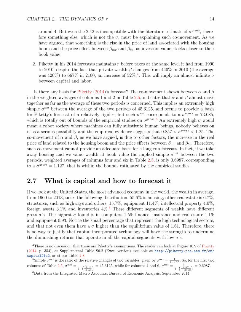
2.7 What is capital and how to forecast it
If we look at the United States, the most advanced economy in the world, the wealth in average,from 1960 to 2013, takes the following distribution: 55.6% is housing, other real estate is 6.7%,structures, such as highways and others, 15.7%, equipment 11.4%, intellectual property 4.0%,foreign assets 3.1% and inventories 4%.6 These different segments of wealth have differentgross σ’s. The highest σ found is in computers 1.59; finance, insurance and real estate 1.16;and equipment 0.93. Notice the small percentage that represent the high technological sectors,and that not even them have a σ higher than the equilibrium value of 1.61. Therefore, thereis no way to justify that capital-incorporated technology will have the strength to underminethe diminishing returns that operate in all the capital segments with low σ’s.
4There is no discussion that these are Piketty’s assumptions. The reader can look at Figure 10.9 of Piketty(2014, p. 354), at Supplemental Table S6.2 (Excel version) available at http://piketty.pse.ens.fr/en/
capital21c2, or at our Table 2.85Simple σnet is the ratio of the relative changes of two variables, given by σnet = 1
1−σαβ . So, for the first two
columns of Table 2.5, σnet = 1
1−(14.1814.50
) = 45.3125, while for columns 4 and 6, σnet = 1
1−(
4.57−10.60
) = 0.6987.
6Data from the Integrated Macro Accounts, Bureau of Economic Analysis, September 2014.
CHAPTER 2. THE DYNAMICS OF r 15
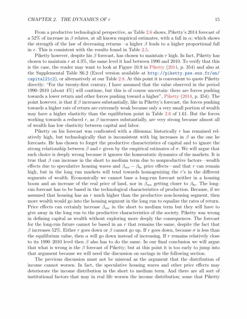
From a productive technological perspective, as Table 2.6 shows, Piketty’s 2014 forecast ofa 52% of increase in β relates, at all known empirical estimates, with a fall in α; which showsthe strength of the law of decreasing returns—a higher β leads to a higher proportional fallin r. This is consistent with the results found in Table 2.5.
Piketty however, despite his β forecast, has chosen to maintain r high. In fact, Piketty haschosen to maintain r at 4.3%, the same level it had between 1990 and 2010. To verify that thisis the case, the reader may want to look at Figure 10.9 in Piketty (2014, p. 354) and also atthe Supplemental Table S6.2 (Excel version available at http://piketty.pse.ens.fr/en/
capital21c2), or alternatively at our Table 2.8. At this point it is convenient to quote Pikettydirectly: “For the twenty-first century, I have assumed that the value observed in the period1990–2010 (about 4%) will continue, but this is of course uncertain: there are forces pushingtowards a lower return and other forces pushing toward a higher”, Piketty (2014, p. 354). Thepoint however, is that if β increases substantially, like in Piketty’s forecast, the forces pushingtowards a higher rate of return are extremely weak because only a very small portion of wealthmay have a higher elasticity than the equilibrium point in Table 2.6 of 1.61. But the forcesworking towards a reduced r, as β increases substantially, are very strong because almost allof wealth has low elasticity between capital and labor.
Piketty on his forecast was confronted with a dilemma: historically r has remained rel-atively high, but technologically that is inconsistent with big increases in β as the one heforecasts. He has chosen to forget the productive characteristics of capital and to ignore thestrong relationship between β and r given by the empirical estimates of σ. We will argue thatsuch choice is deeply wrong because it ignores the homeostatic dynamics of the markets. It istrue that β can increase in the short to medium term due to nonproductive factors—wealtheffects due to speculative housing waves and βmv − βbv price effects—and that r can remainhigh, but in the long run markets will tend towards homogenizing the r’s in the differentsegments of wealth. Economically we cannot base a long-run forecast neither in a housingboom and an increase of the real price of land, nor in βmv getting closer to βbv. The long-run forecast has to be based in the technological characteristics of production. Because, if weassumed that housing has an r much higher than the productive non-housing segment, thenmore wealth would go into the housing segment in the long run to equalize the rates of return.Price effects can certainly increase βmv in the short to medium term but they will have togive away in the long run to the productive characteristics of the society. Piketty was wrongin defining capital as wealth without exploring more deeply the consequences. The forecastfor the long-run future cannot be based in an r that remains the same, despite the fact thatβ increases 52%. Either r goes down or β cannot go up. If r goes down, because σ is less thanthe equilibrium value, then α will go down instead of increasing. If r remains relatively closeto its 1990–2010 level then β also has to do the same. In our final conclusion we will arguethat what is wrong is the β forecast of Piketty; but at this point it is too early to jump intothat argument because we will need the discussion on savings in the following section.
The previous discussion must not be misread as the argument that the distribution ofincome cannot worsen. In fact, the speculative housing waves and other price effects maydeteriorate the income distribution in the short to medium term. And there are all sort ofinstitutional factors that may in real life worsen the income distribution; some that Piketty
CHAPTER 2. THE DYNAMICS OF r 16
comments, like the salaries of the supermanagers in the U.S., and some that he does not, likegrowth, urban, educational and health policies amongst others. There may also be powerfulpolitical forces pushing for policies that may deteriorate the income distribution. Therefore,the society has to be always alert. But Piketty’s dynamics, which implies that there arepowerful long-run economic forces that will necessarily concentrate the income distribution is,as we will show, unsustainable.
2.8 Piketty and Zucman’s arguments in relationship to
the long run
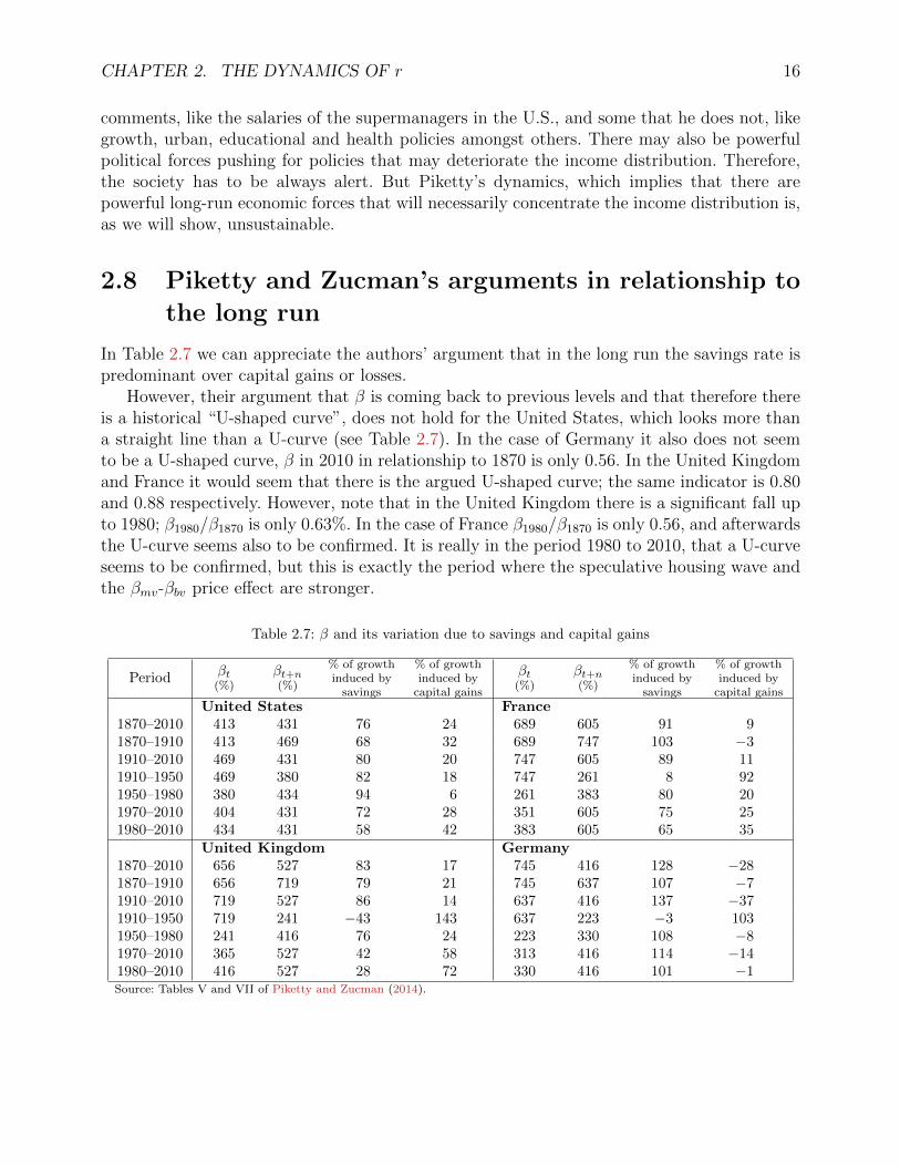
In Table 2.7 we can appreciate the authors’ argument that in the long run the savings rate ispredominant over capital gains or losses.
However, their argument that β is coming back to previous levels and that therefore thereis a historical “U-shaped curve”, does not hold for the United States, which looks more thana straight line than a U-curve (see Table 2.7). In the case of Germany it also does not seemto be a U-shaped curve, β in 2010 in relationship to 1870 is only 0.56. In the United Kingdomand France it would seem that there is the argued U-shaped curve; the same indicator is 0.80and 0.88 respectively. However, note that in the United Kingdom there is a significant fall upto 1980; β1980/β1870 is only 0.63%. In the case of France β1980/β1870 is only 0.56, and afterwardsthe U-curve seems also to be confirmed. It is really in the period 1980 to 2010, that a U-curveseems to be confirmed, but this is exactly the period where the speculative housing wave andthe βmv-βbv price effect are stronger.
Table 2.7: β and its variation due to savings and capital gains
Period βt(%)
βt+n(%)
% of growthinduced by
savings
% of growthinduced by
capital gains
βt(%)
βt+n(%)
% of growthinduced by
savings
% of growthinduced by
capital gains
United States France1870–2010 413 431 76 24 689 605 91 91870–1910 413 469 68 32 689 747 103 −31910–2010 469 431 80 20 747 605 89 111910–1950 469 380 82 18 747 261 8 921950–1980 380 434 94 6 261 383 80 201970–2010 404 431 72 28 351 605 75 251980–2010 434 431 58 42 383 605 65 35
United Kingdom Germany1870–2010 656 527 83 17 745 416 128 −281870–1910 656 719 79 21 745 637 107 −71910–2010 719 527 86 14 637 416 137 −371910–1950 719 241 −43 143 637 223 −3 1031950–1980 241 416 76 24 223 330 108 −81970–2010 365 527 42 58 313 416 114 −141980–2010 416 527 28 72 330 416 101 −1Source: Tables V and VII of Piketty and Zucman (2014).
CHAPTER 2. THE DYNAMICS OF r 17
Table 2.8: Piketty’s historical data
r − g r − g r r g g PopulationPeriod (b. taxes) (a. taxes) (b. taxes) (a. taxes) (%) (per capita, %) (growth, %.)0–1000 4.5 4.5 4.5 4.5 0.01 0.00 0.02
1000–1500 4.4 4.4 4.5 4.5 0.14 0.04 0.101500–1700 4.3 4.3 4.5 4.5 0.20 0.04 0.161700–1820 4.6 4.6 5.1 5.1 0.53 0.07 0.461820–1913 3.5 3.5 5.0 5.0 1.49 0.90 0.561913–1950 3.3 −0.7 5.1 1.1 1.81 0.87 0.931950–2012 1.5 −0.6 5.3 3.2 3.78 2.08 1.672012–2050 1.0 0.6 4.3 3.9 3.28 2.53 0.732050–2100 2.8 2.8 4.3 4.3 1.53 1.33 0.17
Source: Supplementary Tables S2.2, S2.4 and S10.3 of Piketty (2014), available online athttp://piketty.pse.ens.fr/en/capital21c2.
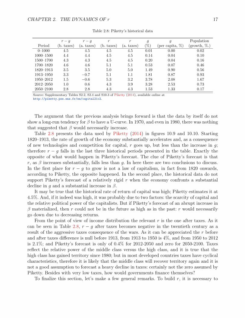
The argument that the previous analysis brings forward is that the data by itself do notshow a long-run tendency for β to have a U-curve. In 1970, and even in 1980, there was nothingthat suggested that β would necessarily increase.
Table 2.8 presents the data used by Piketty (2014) in figures 10.9 and 10.10. Starting1820–1913, the rate of growth of the economy substantially accelerates and, as a consequenceof new technologies and competition for capital, r goes up, but less than the increase in g;therefore r − g falls in the last three historical periods presented in the table. Exactly theopposite of what would happen in Piketty’s forecast. The clue of Piketty’s forecast is thatr, as β increases substantially, falls less than g. In here there are two conclusions to discuss.In the first place for r − g to grow is not a law of capitalism, in fact from 1820 onwards,according to Piketty, the opposite happened. In the second place, the historical data do notsupport Piketty’s forecast of a relatively rigid r when the economy confronts a substantialdecline in g and a substantial increase in β.
It may be true that the historical rate of return of capital was high; Piketty estimates it at4.5%. And, if it indeed was high, it was probably due to two factors: the scarcity of capital andthe relative political power of the capitalists. But if Piketty’s forecast of an abrupt increase inβ materialized, then r could not be in the future as high as in the past: r would necessarilygo down due to decreasing returns.
From the point of view of income distribution the relevant r is the one after taxes. As itcan be seen in Table 2.8, r − g after taxes becomes negative in the twentieth century as aresult of the aggressive taxes consequence of the wars. As it can be appreciated the r beforeand after taxes difference is null before 1913, from 1913 to 1950 is 4%, and from 1950 to 2012is 2.1%; and Piketty’s forecast is only of 0.4% for 2012-2050 and zero for 2050-2100. Taxesreflect the relative power of the middle class versus the high class, and it is true that thehigh class has gained territory since 1980; but in most developed countries taxes have cyclicalcharacteristics, therefore it is likely that the middle class will recover territory again and it isnot a good assumption to forecast a heavy decline in taxes: certainly not the zero assumed byPiketty. Besides with very low taxes, how would governments finance themselves?
To finalize this section, let’s make a few general remarks. To build r, it is necessary to
CHAPTER 2. THE DYNAMICS OF r 18
have statistics of both capital income and capital stock. In relationship to capital incomethere are solid statistics since the Second World War and efforts of government agenciesand academicians to provide much older data. At the world level, however, there is onlyone consistent database since 1990 in the World Bank data, remember that it is needed tohave constant currency international dollars with the same PPP (purchasing power parity).In relationship to capital stock, several countries started serious statistical efforts since the90’s. For example, the United States presents statistics since 1960. However there are notadequate consolidated statistics at the global level. It is true that this is one of the reasonsfor which Piketty’s work is so welcome, he does indeed a serious and professional job to definea comparable capital stock at the world level. He is particularly successful in France, theU.K. and to a large extent in the U.S. But it is also true that many statistics are difficultto consolidate and that their consolidation requires many assumptions. Just to remind thereader in something as simple as the growth of the economy, Maddison and the World Bankdiffer seriously in periods as close as the 90’s.7 Therefore, in Piketty, one could probably arguethat data for 1970 to 2012 is pretty solid and that it is quite acceptable for the eighteenthand nineteenth centuries in France, the U.K. and the U.S. But the inference to the world levelthat Piketty makes out of such data is likely less acceptable.
Piketty’s guess as to the level of the long-run historical rate of return of capital at theworld level is precisely that, only an educated guess which has merit but does not haveadequate empirical support. Therefore, his argument that r is relatively stable in the verylong run is at least susceptible of conceptual discussion. It seems to us that his argumentis questionable, because as the wealth forms change, the relationship between r and othervariables changes; and therefore there is not a meaningful comparison between diverse culturesin distinct historical periods. In autocratic societies r could be relatively rigid due to the highrelative power of the autocracy, in democracies such power subsists but it is reduced; and themarkets expansion gives the productive capital a new logic—very different in nature to the oldsumptuous palaces or Egyptians pyramids. Productive capital’s expansion necessarily relatesto the decreasing returns logic and r becomes inversely related to the size of β.
In summary, 75 years of empirical work show that the elasticity between capital and laboris less than 1.25. Rognlie shows that housing explains 80% of the β increase in the period1970 to 2010. We have shown that if we remove housing and using β at book value, for allthe countries there is an inverse relationship between α and β. Piketty’s notion that β indeveloped countries has a historical U-shaped curve is not corroborated by data. Most of theβ increase from 1970 to 2010 is related to the housing boom, the increase in land prices andto price effects between βmv and βbv. But these speculative waves and price effects cannotbe a solid base for a long-run forecast. Markets will tend to homogenize the rates of returnamongst diverse wealth sectors; therefore the logic of the forecasted relationship between α
7In the period of 1990 to 2000: for the world, Maddison reports 1.6% average annual growth and the WorldBank 3.04% (the difference being influenced by their distinct estimates about the growth of China); for theUnited States the corresponding values are 2.5% and 3.2%, for the United Kingdom 2.5 and 3.2; for Germany1.75% and 1.4%; they are only similar for France, 2.0% and 2.1% respectively. The World Bank reports grossand net savings rates since 1970, for France and the world only from 1975; but it only reports g, which requiresconstant PPP international dollars, since 1990. Maddison reports g since 1970, and even since the year one,but he does not have estimates of the gross and net savings rates.
CHAPTER 2. THE DYNAMICS OF r 19
and β has to be rooted in the productive characteristics of capital. The forecasts have to bein accordance with the empirical findings as to the value of σ.
What will happen in the real world? It is impossible to forecast it, reality can always besubject to speculative movements and short-term price effects. And what will actually happendepends critically in the institutional policies that will be adopted. But from the point of viewof theoretical forecasting between two stationary states, we have to be based in the underlyingproductive forces, leaving aside short to medium term movements which cannot be forecasted.In the long run the law of decreasing returns must operate, as the markets homogenize ther along segments, in all the wealth; therefore, as β increases substantially there is a higherproportional fall in r, and there must be an inverse relationship between α and β.
Finally, let us focus on what could be an alternative scenario for r, assuming Piketty’ssubstantial increase in β, r should be substantially lower, in the range between 1.55% and2.42%—these estimates are based upon σ = 0.857, and σ = 1.25. And now let us imagine thattaxes remain at 30%. Then r after taxes could be as low as 1.09% to 1.69%, and r − g couldbe negative or very small.
The range of r before taxes of 1.55% to 2.42% seems very low compared to its historicalvalues. This is due to the fact that Piketty forecasts a substantial increase in β, of 52%, and theabundance of capital awakens strong decreasing returns which in turn lower r significantly.How much can we trust Piketty’s forecast that there will be a substantial increase in β?To answer this question appropriately we will need to go into the next section, where wewill explore the relationship between the net savings rate and the real rate of growth of theeconomy, the determinants of the level of β.
Chapter 3
The dynamics of s
As we have mentioned, the relative rigidity of the net savings rate is also fundamental inPiketty’s proposal of capitalism dynamics. Piketty and Zucman (2014, pp. 15–16) argue thattheir theory is valid for diverse economic growth models, including the dynastic, in which sis a positive function of g. They point out that as long as s moves less than g, β remainsa positive function of g. Moreover, they say that there does not seem to be a relationshipbetween s and g, during 1970-2010, when comparing across developed economies (see Table2.1). These two arguments have been questioned by Krusell and Smith (2015).
The apparent inexistent s and g relation, they argue, is due to institutional differencesbetween the countries. Using postwar U.S. data they show that there is a positive relationshipbetween s and g and that it is strong enough so that as g goes down only small increases inβ are obtained. Their results contradict Piketty’s forecast that β will substantially increasein the twenty-first century. They also show that Piketty’s economic growth model showskey differences with Solow’s textbook model as well as with models of endogenous savingoptimization.8
8Krusell and Smith, using a constant net savings rate to describe Piketty’s model and a production functionwith labor augmented technology, show that the following relations are different in Piketty’s stationary stateversus the traditional Solow model in textbooks. Gross and net variables are denoted with subindices b and n,
respectively. I) Gross consumption/gross income, CbYb
, in Solow is 1 − sb, in Piketty is (1−sn)g(g+snδ)
(where g is the
real rate of growth of the economy and δ is the capital depreciation rate). Therefore, in Piketty a lower g isassociated with a lower gross consumption/gross income ratio. II) In Piketty the relation between sb and sn is
given by sb = sn(g+δ)g+snδ
, therefore with sn fixed, sb goes up aggressively when g falls. In the traditional model,
sn and sb are related by the equation sn = gsbg+δ(1−sb) ; therefore, with sb given from outside and constant, when
g falls, sn also falls, and when g goes to zero sn also goes to zero. Thus, except for the non-interesting case ofsb = 1, sn is a positive function of g. III) K
Ybin Solow’s model is sb
(g+δ) , and in Piketty’s is sn(g+snδ)
; KYn
= sng in
Piketty (his second fundamental law) and in Solow KYn
= sbg+δ(1−sb) .
The consequences are: a) In Piketty with sn constant, when g goes to zero Cb/Yb in Piketty goes to zero;therefore sb goes to 1; b) K
Yn= sn
g in Piketty goes to infinity as g goes to zero. While in the traditional modelKYn
= sbg+δ(1−sb) , therefore, when g goes to zero K
Ynhas a limit sb
δ(1−sb) ; this limit, using standard values for the
world economy of sb = 0.2298 and δ = 0.0367—average values from 1990 to 2010—will be 8.12. (c) KYb
has a
limit in both cases; in the traditional model the limit will be sbδ = 6.26; and in Piketty 1
δ = 27.23. d) In thetraditional model, changes in sb take the economy to a new higher growth path and to an increase in K. Kin the traditional model, however, cannot grow without bound, because its growth is finally conditioned by
20
CHAPTER 3. THE DYNAMICS OF s 21
3.1 Solow vs. Piketty. Conceptual differences
In Solow’s textbook model the net savings rate is given by the equation sn = gsbg+δ(1−sb)
, andKYn
by the expression KYn
= sbg+δ(1−sb)
. Where sb is the gross savings rate and δ is the capital
depreciation rate. Manipulating the previous expressions one easily obtains KYn
= sng
, Piketty’ssecond fundamental law. However, despite its mathematical identity, conceptual differencesremain. In Solow sb is exogenously given while in Pikkety sn is assumed relatively rigid. InSolow sn is a positive function of g. In Solow when g goes to zero there is a limit for K
Yngiven
by sbδ(1−sb)
. In Piketty with sn relatively rigid when g goes to zero mathematically KYn
goes toinfinity – the argument Krusell and Smith have been insisting on; in fact, in economic termsKYn
will be restricted in a pikettian economy by the fact that α cannot be greater than one,but anyway it is an unreasonable result. While in Solow sb is given from outside; in Piketty,with sn relatively rigid, sb increases unbounded, since in Piketty’s model sb = sn(g+δ)
g+snδ.
Using the average historical values for the world economy from 1990 to 2010, sb = 22.979%and the estimated capital depreciation rate δ = 0.0367, Table 3.1, compares at several valuesfor g, Solows equation, K
Yn= sb
g+δ(1−sb), with Piketty’s second fundamental law, assuming for
Piketty a fixed sn = 10%. As it can be seen as g becomes very low K/Yn in Solow tends toits limit, at the values used, of 8.12; while in Piketty it grows unbounded—the point madeby Krusell and Smith. In addition as g goes to zero sn goes to zero in Solows model. Butsb in Piketty’s increases unbounded; which is particularly problematic, because at g = 1.5%,the value of his forecast, sb would be equal to 27.70%, but this value is too high for anyhistorical period of the world economy; data is available since 1975, and at no single year ithas been higher than 25, and the average 1975–2012 was 23.14. Thus, it clearly shows thatthe sn = 10% of Piketty is too high. Also in Piketty β is more sensitive to g movements, sowhen g halves from 3% to 1.5%, β in Piketty doubles, while in Solow it only increases 34.8%.Finally, Solow’s β forecast at g = 1.5% is significantly lower than Pikkety’s. Notice that snin Solow is a positive function of g, therefore as g goes down to 1.5% sn goes also down to7.96%, that is why Solow’s forecast is lower than Piketty’s.
Solow’s model in Table 3.1 is an improvement in Piketty’s, because sn becomes a functionof g. However, it must be noticed that since sb is given from outside, sb is not a function of g.
the law of diminishing returns which says that as capital goes to infinity its marginal product goes to zero—what is known as the Inada condition. In Piketty instead, the change in the net product can be expressed asF (K, ·)− δK, and while F (K, ·)− δK also satisfies the Inada condition, F (K, ·) does not; that is why K
Yngoes
to infinity as g goes to zero. The clue is that while in the traditional model the decreasing return falls belowthe depreciation rate and stops the growth of capital; in Piketty with an almost fixed high return, capitalreturns are always high enough for capital to grow unbounded towards the infinity. In economic terms theβ growth will be restricted to the value at which capitalists own 100% of income, but it is anyhow a veryunsatisfactory result. It is worth pointing out that Krusell and Smith, in their article, use a very high andunsustainable capital depreciation rate of 8%.
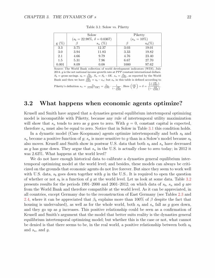
CHAPTER 3. THE DYNAMICS OF s 22
Table 3.1: Solow vs. Piketty
Solow Piketty(sb = 22.98%, δ = 0.0367) (sn = 10%)
g (%) β sn (%) β sb(%)3.3 3.75 12.37 3.03 19.013.0 3.94 11.83 3.33 19.822.1 4.66 9.79 4.76 23.401.5 5.31 7.96 6.67 27.70
0.001 8.09 0.08 1000 97.62Source: The World Bank collection of world development indicators (WDI), July2014. g is the net national income growth rate at PPP constant international dollars.
Sb = gross savings. sb = SbGNI
. Sn = Sb − δK. sn = SnGNI
, as reported by the World
Bank and then we have δKGNI
= sb − sn; but sn in this table is defined according to
Piketty’s definition sn = Sn(GNI−δK)
= SnGNI
· 1
1− δKGNI
. Here(δKK
)= δ =
1β
(δKGNI
)(1− δK
GNI
) .
3.2 What happens when economic agents optimize?
Krusell and Smith have argued that a dynasties general equilibrium intertemporal optimizingmodel is incompatible with Piketty, because any rule of intertemporal utility maximizationwill show that sn tends to zero as g goes to zero. With g = 0, constant capital is expected,therefore sn must also be equal to zero. Notice that in Solow in Table 3.1 this condition holds.
In a dynastic model (Cass–Koopmans) agents optimize intertemporally and both sb andsn become a positive function of g; sn is more sensitive to g than in a Solow’s model because sbalso moves. Krusell and Smith show in postwar U.S. data that both sb and sn have decreasedas g has gone down. They argue that sn in the U.S. is actually close to zero today; in 2012 itwas 2.63%. What happens at the world level?
We do not have enough historical data to calibrate a dynasties general equilibrium inter-temporal optimizing model at the world level; and besides, these models can always be criti-cized on the grounds that economic agents do not live forever. But since they seem to work wellwith U.S. data, sb goes down together with g in the U.S.. It is required to open the questionof whether or not sb is a function of g at the world level. Let us look at some data. Table 3.2presents results for the periods 1991–2000 and 2001–2012; on which data of sb, sn and g arefrom the World Bank and therefore compatible at the world level. As it can be appreciated, inall countries, except Germany due to the reconstruction of East Germany (see Tables 2.3 and2.4, where it can be appreciated that βh explains more than 100% of β despite the fact thathousing is undervalued), as well as for the whole world, both sb and sn fall as g goes down,and they go up as g increases. This positive relationship could be seen as a confirmation ofKrusell and Smith’s argument that the model that better suits reality is the dynasties generalequilibrium intertemporal optimizing model; but whether this is the case or not, what cannotbe denied is that there seems to be, in the real world, a positive relationship between both sband sn, and g.
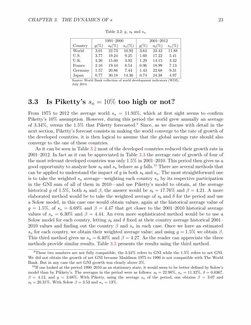
CHAPTER 3. THE DYNAMICS OF s 23
Table 3.2: g, sb and sn
1991–2000 2001–2012Country g(%) sb(%) sn(%) g(%) sb(%) sn(%)World 3.01 22.73 10.92 3.64 23.42 11.88U.S. 3.77 19.24 9.25 1.60 17.22 5.41U.K. 3.26 15.60 3.92 1.29 14.15 3.32France 2.16 19.44 8.54 0.96 18.99 7.13Germany 1.57 20.86 7.44 1.43 22.68 9.31Japan 0.77 30.18 14.36 0.74 24.38 4.97
Source: World Bank collection of world development indicators (WDI),July 2014.
3.3 Is Piketty’s sn = 10% too high or not?
From 1975 to 2012 the average world sn = 11.93%, which at first sight seems to confirmPiketty’s 10% assumption. However, during this period the world grew annually an averageof 3.34%, versus the 1.5% that Piketty forecasted.9 Since, as we discuss with detail in thenext section, Piketty’s forecast consists in making the world converge to the rate of growth ofthe developed countries, it is then logical to assume that the global savings rate should alsoconverge to the one of these countries.
As it can be seen in Table 3.2 most of the developed countries reduced their growth rate in2001–2012. In fact as it can be appreciated in Table 3.3 the average rate of growth of four ofthe most relevant developed countries was only 1.5% in 2001–2010. This period then gives us agood opportunity to analyze how sb and sn behave as g falls.10 There are several methods thatcan be applied to understand the impact of g in both sb and sn. The most straightforward oneis to take the weighted sn average—weighting each country sn by its respective participationin the GNI sum of all of them in 2010—and use Piketty’s model to obtain, at the averagehistorical g of 1.5%, both sb and β, the answer would be sb = 17.76% and β = 4.21. A moreelaborated method would be to take the weighted average of sb and δ for the period and usea Solow model, in this case one would obtain values, again at the historical average value ofg = 1.5%, of sn = 6.69% and β = 4.47 that get closer to the 2001–2010 historical averagevalues of sn = 6.30% and β = 4.44. An even more sophisticated method would be to use aSolow model for each country, letting sb and δ fixed at their country average historical 2001–2010 values and finding out the country β and sn in each case. Once we have an estimatedsn for each country, we obtain their weighted average value; and using g = 1.5% we obtain β.This third method gives us sn = 6.40% and β = 4.27. As the reader can appreciate the threemethods provide similar results. Table 3.3 presents the results using the third method.
9These two numbers are not fully compatible, the 3.34% refers to GNI while the 1.5% refers to net GNI.We did not obtain the growth of net GNI because Maddison 1975 to 1990 is not compatible with The WorldBank. But in any case the net GNI growth was clearly above 3%.
10If one looked at the period 1990–2010 as an stationary state, it would seem to be better defined by Solow’smodel than by Pikkety’s. The averages in the period were as follows: sb = 22.98%, sn = 11.32%, δ = 0.0367,β = 4.12, and g = 3.68%. With Piketty, using the average sn of the period, one obtains β = 3.07 andsb = 20.31%. With Solow β = 3.53 and sn = 13%.
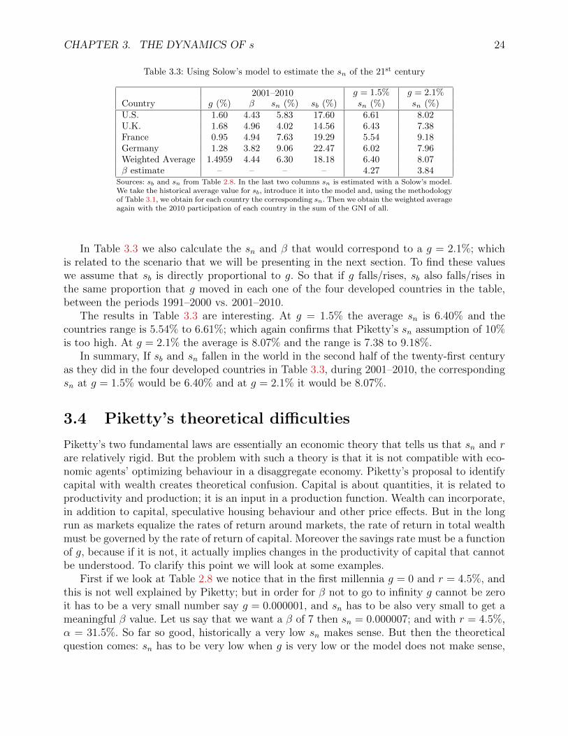
CHAPTER 3. THE DYNAMICS OF s 24
Table 3.3: Using Solow’s model to estimate the sn of the 21st century
2001–2010 g = 1.5% g = 2.1%Country g (%) β sn (%) sb (%) sn (%) sn (%)U.S. 1.60 4.43 5.83 17.60 6.61 8.02U.K. 1.68 4.96 4.02 14.56 6.43 7.38France 0.95 4.94 7.63 19.29 5.54 9.18Germany 1.28 3.82 9.06 22.47 6.02 7.96Weighted Average 1.4959 4.44 6.30 18.18 6.40 8.07β estimate – – – – 4.27 3.84
Sources: sb and sn from Table 2.8. In the last two columns sn is estimated with a Solow’s model.We take the historical average value for sb, introduce it into the model and, using the methodologyof Table 3.1, we obtain for each country the corresponding sn. Then we obtain the weighted averageagain with the 2010 participation of each country in the sum of the GNI of all.
In Table 3.3 we also calculate the sn and β that would correspond to a g = 2.1%; whichis related to the scenario that we will be presenting in the next section. To find these valueswe assume that sb is directly proportional to g. So that if g falls/rises, sb also falls/rises inthe same proportion that g moved in each one of the four developed countries in the table,between the periods 1991–2000 vs. 2001–2010.
The results in Table 3.3 are interesting. At g = 1.5% the average sn is 6.40% and thecountries range is 5.54% to 6.61%; which again confirms that Piketty’s sn assumption of 10%is too high. At g = 2.1% the average is 8.07% and the range is 7.38 to 9.18%.
In summary, If sb and sn fallen in the world in the second half of the twenty-first centuryas they did in the four developed countries in Table 3.3, during 2001–2010, the correspondingsn at g = 1.5% would be 6.40% and at g = 2.1% it would be 8.07%.
3.4 Piketty’s theoretical difficulties
Piketty’s two fundamental laws are essentially an economic theory that tells us that sn and rare relatively rigid. But the problem with such a theory is that it is not compatible with eco-nomic agents’ optimizing behaviour in a disaggregate economy. Piketty’s proposal to identifycapital with wealth creates theoretical confusion. Capital is about quantities, it is related toproductivity and production; it is an input in a production function. Wealth can incorporate,in addition to capital, speculative housing behaviour and other price effects. But in the longrun as markets equalize the rates of return around markets, the rate of return in total wealthmust be governed by the rate of return of capital. Moreover the savings rate must be a functionof g, because if it is not, it actually implies changes in the productivity of capital that cannotbe understood. To clarify this point we will look at some examples.
First if we look at Table 2.8 we notice that in the first millennia g = 0 and r = 4.5%, andthis is not well explained by Piketty; but in order for β not to go to infinity g cannot be zeroit has to be a very small number say g = 0.000001, and sn has to be also very small to get ameaningful β value. Let us say that we want a β of 7 then sn = 0.000007; and with r = 4.5%,α = 31.5%. So far so good, historically a very low sn makes sense. But then the theoreticalquestion comes: sn has to be very low when g is very low or the model does not make sense,
CHAPTER 3. THE DYNAMICS OF s 25
but then this implies that sn must move with g.We need a theory that links sn with g, and just arguing that sn is relatively rigid is not
good enough. In Solow’s model, sb is given from outside and the model explains that a highersb is related to a higher growth path, one associated with a higher initial income per capita.Once we are in the growth path any income per-capita growth is compatible with any sn,but initially the whole purpose of increasing sb was to move to a higher growth path. Savingmust have a productive purpose. One cannot just move sn without understanding what isthe economic theoretical productive story that is related to such an increase. The followingexample will bring this point forward.
Let us imagine two stationary states X and Z. Let us assume that population does notgrow in neither of them, that we have full employment and that the labor force that we denoteby LF , to distinguish it from labor income L, does not grow either and it is the same in botheconomies. Let us make income the numeraire, Y = 1. The stationary state X reproducesPiketty’s forecast for the second half of the twenty-first century with sn = 10%, r = 4.3%and g = 1.5%; therefore β = 6.7 and α = 28.7%. The stationary state Z will be definedas a function of the long-term interest of the capitalists. Since the capitalists have controlupon the net savings rate, sn, the question is, What happens if they raise it from 10% to20%? The answer in a Pikettian economy is that β = 13.33, and α = 0.573. Since Y = 1,then C = α. The capitalists will optimize then the present discounted value of their income,which we will denote by Cpv. In general terms Cpv = α
r−g ; the value of an infinite series withan initial value α which grows at g and is discounted at r. Then for the stationary stateX; Cpv = 0.287
0.043−0.015= 10.25. And for the stationary state Z; Cpv = 0.573
0.043−0.015= 20.46. It
means that the capitalists not only increase their share in total income but also the presentdiscounted value of their income. Since sn is to be decided by the capitalists then they shouldincrease it until they obtain the maximum possible income. Note that α = rsn
0.015, therefore if
α = 1, then sn = 0.0150.043
= 0.349; which means that if the capitalist save 34.9%, they will own100% of the national income.
In fact they will be restricted by the minimum subsistence salary that they would needto give to the labor force. Let w equal the subsistence salary, then w · LF = L, the laborincome. And the share of labor in income will be L/Y = L. α then will be 1 − L. The snwhich optimizes Cpv is the one that gives as a solution α = 1 − L. Since Cpv is an increasingmonotonic function of sn (because Cpv = s × 102.38), Cpv always grows as sn grows. Thus,to maximize Cpv, sn will grow until α = 1 − L. But since LF does not grow and P , thepopulation, neither, then g = G/P = G, where G is the product growth in real terms. Sincew is a subsistence salary expressed in real terms it does not grow either, therefore w ·LF doesnot grow. Thus, as time t goes to infinity, w·LF
Ygoes to zero and α = 1 − w · LF goes to 1;
therefore sn goes to the limit of 34.9% and Cpv goes to 35.7%.In summary, the problem with Piketty’s economic dynamics is that it would imply that
in the long run, if the capitalists maximize their interest, they will have all the income of theeconomy. A result which is not very interesting and clearly difficult to defend.
Of course it could be argued against the previous intellectual exercise that the capitalistsdo not calculate their interest in the infinite horizon. But the point of the exercise is not toargue that they do, the purpose is to expose the theoretical problems of Piketty’s proposal. In
CHAPTER 3. THE DYNAMICS OF s 26
Piketty’s proposal economic agents do not optimize, in fact if they do his theoretical modelis unsustainable. It is not possible to develop a theoretical model of income distribution asPiketty pretends without having both r and s linked theoretically to the production processof the economy. The reason, in the real world, why capitalist do not increase their saving somuch is because they face decreasing returns. In Piketty, with r relatively rigid the capitalistscan increase s and always increase their income share; in a productive economy they cannotbecause of diminishing returns.
3.5 What is the problem? Another example to further
understand what is happening
Let us imagine again an economy with zero population growth and that LF is constant andit is the numeraire, then LF = 1. And let us assume that the initial product per capitais 2, thus the product Y = 2. If g = 0.01 and sn = 0.05, then β = 5 and K = 10. Theproduction technique in such economy is 10K and 1L produce 2Y . In the second period theproduction technique will be 10.1K and 1L producing 2.02Y and so on. What happens if gfalls to g = 0.001? Then β = 50 and K = 100. The production technique is now such that100K and 1L produce 2Y . And in the second period 100.1K and 1L produce 2.002Y , and soon. What happened that the economy needs much more capital to produce the same product?K/Y increasing means that capital productivity is going down, and then there is the need tohave a productive story of why this happens: Piketty does not have it. K/Y movements donot only relate to an income distribution story, they also are necessarily related to a story ofthe productivity of capital—a story that Pikety never develops.
It is true that once in a growth path, two stationary states can have the same g anddifferent sn, but the level of such growth paths is given by the difference in the initial push ofthe difference in savings rates. In addition if K goes up, as we saw in the previous section rmust go down.
The relative rigidity in r and sn that Piketty introduces causes all kind of theoretical non-sense stories, we already saw that as g goes to zero β goes to infinity and sb grows unbounded,but also notice that as β grows a lot, for example if it reaches 50, α would be equal to 215%.Thus or β grows less or r falls or both things happen.
That g falls does not necessarily must imply that K/Y must go up. If sn falls proportionallyto g, then sn would be equal to 0.005, and β would be again equal to 5 and K = 10. Thetechnique of production then is not modified, and the productivity of capital remains thesame.
From a productive point of view, the only reason for capital to go up to 100 would have tobe that it is associated with a considerable increase in initial Y , so that initial Y/L, the level ofthe growth path, is substantially higher. The K level is not linked to g, but it has to be to theinitial per capita product. How much would initial Y have to go up in the previous example?To solve this, suppose the terminal r used by Piketty of 0.043. When g = 0.01 we can observethat the product present discounted value, Ypv, is
(2
0.043−0.01
)= 60.606, and capital present
discounted value, Kpv, is(
100.043−0.01
)= 303.03. There are no surprises and K/Y is then 5.
CHAPTER 3. THE DYNAMICS OF s 27
What we want to find is the value of initial Y such that when g = 0.001, K/Y stays in 5. Inorder to do that, observe that Kpv is now
(100
0.043−0.01
)= 2380.95 . Therefore Ypv would have to
be equal to 476.19 for K/Y to remain in 5. Now if Ypv is 476.19, then no surprises, the initialY has to be 20—this result is of course general at any level of r.
Then as g falls from 0.01 to 0.001 one of three things needs to happen, or a combinationof them: 1) s falls proportionally to g and K/Y remains unchanged, 2) K goes up and theeconomy moves into a new growth path in which initial Y also goes up and therefore K/Yremains unchanged (notice in here that g may be the same as before but it starts from aninitial higher Y ), 3) K/Y goes up. But in this third alternative it is necessary to explainwhy the productivity of capital goes down. 1) is not compatible with Piketty’s assumption ofa relatively rigid sn; 2) is not compatible with Piketty because he assumes that the growthrate of the developed countries goes down starting 2012. And there is never a discussion as tothe transitional consequences on economic growth related to the increase in β. Therefore, inPiketty, initial Y never goes up. Then, 3) is Piketty’s selected option. But then an explanationis needed of why the productivity of capital is going down, particularly with the increase in βof 50% forecasted by this author, but he never provides such explanation.
For β to go up 50% one of two explanations has to be provided: 1) the productivity ofcapital goes down dramatically, or 2) the increase is explained by speculative housing wavesand/or price effects. But 2), as we have been arguing is only valid in the short to mediumterm, moreover Piketty does not have an explanation of this type either. And 1) is just notbelievable, because there is no reason for capital to become so unproductive. Moreover, if itdid then the rate of return on capital, r, should also go down dramatically—and as we saw inthe previous section, a higher β leads to a higher proportional fall in r.
It must be noticed that the direct relationship between sb and sn with g should not nec-essarily hold for any period and for any country, if a country chooses to increase his savingsrate in order to foster a higher future transitional growth for a given period, sb and sn mayincrease with g going down, so the relationship can be inverse temporarily as it happens withGermany in Table 3.2. The high sn in Germany as we said is due to the reconstruction ofEast Germany. But when comparing stationary states in which sn remains fixed at the levelrequired in each stationary state, the relationship must be necessarily direct, unless a highersn can be related to a previous higher transitional growth, which is not the case with Piketty’sforecast.
Also it must be pointed out that while it is true that the long-run growth in westerncapitalism cannot be explained only for higher savings rates, and therefore the expansionof knowledge must be introduced (and it explains most of the growth); that does not meanthat any level of sn can go with any level of g. The purpose of saving is always a highertransitional growth. Besides, for some countries higher savings were absolutely crucial in theirdevelopment, the Asian miracle cannot be explained without high savings.
For Piketty there can be different stationary states with similar saving levels but diverseg’s, which will then be traduced into also different β’s. In what follows we will quote a longparagraph from Piketty because it is crucial to understand his logic: “In other words, for asavings rate on the order of 10–12 percent and a growth rate of national income per capitaon the order of 1.5–2 percent a year, it follows immediately that a country that has near zero
CHAPTER 3. THE DYNAMICS OF s 28
demographic growth and therefore a total growth rate in the order 1.5–2 percent, as in Europe,can expect to accumulate a capital stock worth six to eight years of national income, whereas acountry with demographic growth in the order of I percent a year and therefore a total growthrate of 2.5–3 percent, as in the United States, will accumulate a capital stock worth only threeto four years of national income. And if the latter country tends to save a little less than theformer, perhaps because its population is not aging as rapidly, this mechanism will be furtherreinforced as a result. In other words, countries with similar growth rates of income per capitacan end up with very different capital/income ratios simply because their demographic growthrates are not the same. This allows us to give good account of the historical evolution of thecapital/income ratio.” Piketty (2014, p. 167).
How should we read the previous paragraph? Given the savings rate, everything he affirmsis correct. But the problem is that sn is a function of g, therefore it does not make senseto maintain it fixed, or almost fixed, as one makes the comparison that he does. To furtherenhance our argument we will introduce another example.
Let us imagine an economy where everybody works and initially LF = 1, but it growsat 0.02, g = 0.01, sn = 0.05 and Y/L = 2. Then, again β = 5 and K = 10. But g canbe decomposed in 0.5 productivity and 0.02 population growth. The production techniquewill be 10K and 1L produce 2Y and in the second period 10.1K and 1.02L produce 2.02Y ,and so on. If we reduce the demographic growth rate to 0.01, g will be equal to 0.005; andif we maintain s = 0.05, then β = 10 and K = 20. Piketty’s forecast holds, β grows andthe income distribution deteriorates because the fall in the demographic growth. But noticewhat happened, the new technique of production is 20K and 1L produce 2Y and in the secondperiod 20.1K and 1.01L produce 2.01Y , and so on. Therefore, capital is only half as productiveas before. If we want to maintain the same capital productivity as previously, which meansa constant K/Y , then the savings rate must go down proportionally to g. If the savings rategoes down to 0.025, then technology will remain the same, β = 5 and K = 10; and theproduction technique in the first and subsequent periods does not change. In the first period10K and 1L produce 2Y and in the second period 10.05K and 1.01L produce 2.01Y , and soon. Note that 10.05 : 2.01 :: 10.1 : 2.02. Observe, that if there is less demographic growth, forthe productivity of capital to remain the same, sn has to go down proportionally to g, andthen β remains the same. If β changes it has to be related to productivity story or to an initialchange in the output per worker which would mean a higher transitory growth. Since Pikettydoes not contemplate a higher transitory growth, then his β increase has to be related to lessproductive capital. But then he does not have an answer for why capital is less productive.And also, as we mentioned, if for any reason capital became less productive, then one couldn’tassume a rigid r as he does.
What deteriorates the income distribution in Piketty’s example is not the fall in the rateof demographic growth, but the fact that he maintains sn rigid, or almost rigid. And this snrigidity, as g falls, is necessarily linked to less productive capital and he never discusses orexplains what the source of the reduced productivity is.
Maybe the most important figure in Piketty (2014) is 5.8, which shows the historicaltendency of β and its forecast at the world level. The forecast in Figure 5.8 is a simulationthat goes from the actual β value in 2010, 440, to the value forecasted for 2100, 667. Table
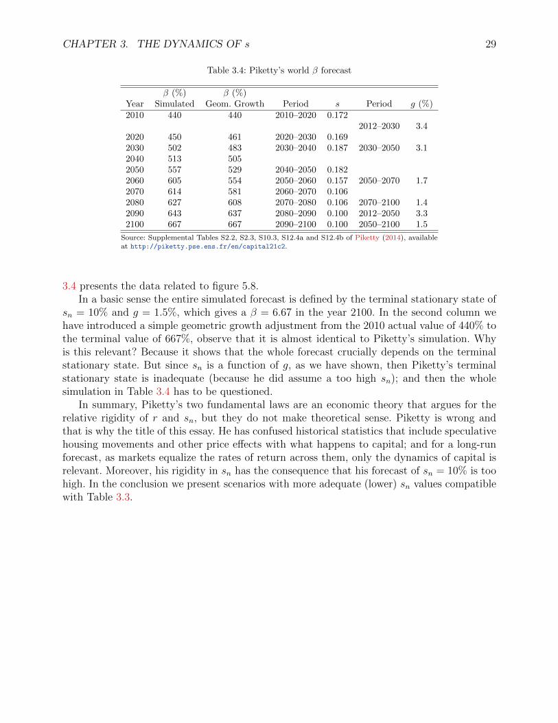
CHAPTER 3. THE DYNAMICS OF s 29
Table 3.4: Piketty’s world β forecast
β (%) β (%)Year Simulated Geom. Growth Period s Period g (%)2010 440 440 2010–2020 0.172
2012–2030 3.42020 450 461 2020–2030 0.1692030 502 483 2030–2040 0.187 2030–2050 3.12040 513 5052050 557 529 2040–2050 0.1822060 605 554 2050–2060 0.157 2050–2070 1.72070 614 581 2060–2070 0.1062080 627 608 2070–2080 0.106 2070–2100 1.42090 643 637 2080–2090 0.100 2012–2050 3.32100 667 667 2090–2100 0.100 2050–2100 1.5
Source: Supplemental Tables S2.2, S2.3, S10.3, S12.4a and S12.4b of Piketty (2014), availableat http://piketty.pse.ens.fr/en/capital21c2.
3.4 presents the data related to figure 5.8.In a basic sense the entire simulated forecast is defined by the terminal stationary state of
sn = 10% and g = 1.5%, which gives a β = 6.67 in the year 2100. In the second column wehave introduced a simple geometric growth adjustment from the 2010 actual value of 440% tothe terminal value of 667%, observe that it is almost identical to Piketty’s simulation. Whyis this relevant? Because it shows that the whole forecast crucially depends on the terminalstationary state. But since sn is a function of g, as we have shown, then Piketty’s terminalstationary state is inadequate (because he did assume a too high sn); and then the wholesimulation in Table 3.4 has to be questioned.
In summary, Piketty’s two fundamental laws are an economic theory that argues for therelative rigidity of r and sn, but they do not make theoretical sense. Piketty is wrong andthat is why the title of this essay. He has confused historical statistics that include speculativehousing movements and other price effects with what happens to capital; and for a long-runforecast, as markets equalize the rates of return across them, only the dynamics of capital isrelevant. Moreover, his rigidity in sn has the consequence that his forecast of sn = 10% is toohigh. In the conclusion we present scenarios with more adequate (lower) sn values compatiblewith Table 3.3.
Chapter 4
The dynamics of g
Piketty argues that economic growth in the twenty-first century will decelerate because growthin the twentieth century was due to two specific temporary phenomena: 1) The two warsreconstruction, and 2) The developing countries convergence. The first will not repeat itself,and the second will continue in the twenty-first century, but only in the first half becausesuch convergence will happen rapidly. Therefore, the world will enter in the second half of thetwenty-first century in what he has called the end of growth. For Piketty long-term growth isexplained by the diffusion of knowledge, a public good, and the convergence between countriesis due to the diffusion of such knowledge. For the second half of the twenty-first century heforecasts lower growth based on three assumptions: 1) a fall in the population growth rate; 2)a fall in the per capita income growth in developed countries; 3) the convergence of developingcountries with developed ones will occur in the first half of the twenty-first century; thereforethere is a positive effect in the rate of growth of the world economy in the first half that willdissipate in the second half.
The fall in the global population growth rate closely follows the United Nations forecastand it seems acceptable to us. But the other two assumptions are questionable.
The argument of the transitory effect of the two wars in the GDP per capita growth rateof developed countries seems unsustainable. The developed world growth rate from 1970–2012was similar to 1913–2012 and was around 1.8%, much higher than Piketty’s 1.2% (see Table4.2); and by 1970 the wars reconstruction effects were mostly over. Therefore, without thewars argument, the only remaining explanation for the drastic fall in g is the deceleration oftechnology, which is highly unlikely.
As to the argument of the rapid convergence of the developing countries, it also seemsinadequate. If the convergence occurred, it would have to be slower than what he forecasts.Therefore, the convergence process will continue in the second half of the twenty-first century.Thus, it is highly unlikely that the world economic growth rate will substantially fall in thesecond half in relation to the first half as he proposes. In fact, if Piketty’s forecast material-ized, it would mean, as we will show, the end of poverty and of the highly unequal incomedistribution among countries; we identify both outcomes as low probability events.
In what follows we will review the historical economic growth data for developed anddeveloping economies and we will build an alternative scenario. The purpose is not to argue
30

CHAPTER 4. THE DYNAMICS OF g 31
that our scenario is more likely than Piketty’s one, because at almost 100 years away it isimpossible to forecast what will really happen. The purpose is to show that Piketty’s forecastis not sustainable, based only upon data, and that his theoretical conjectures are highlyquestionable.
4.1 The deceleration of growth in developed countries
Pikkety proposes that in the rest of the twenty-first century Western Europe, North America,Japan and Australia will grow only 1.2% (see Table 4.1). However these regions and coun-tries grew from 1970–2012 more than 1.8%, almost the same as 1913–2012. They achievedthis growth even though the reconstruction was mostly over and despite the 2008 financialcrisis (see Table 4.2). Therefore the war reconstruction argument to defend the announceddeceleration has little support.
Table 4.1: Economic Growth in the 21st century (GDP per capita growth, Annual %)
Piketty’s scenario Proposed scenarioCountry or Region 2012–2050 2050–2100 2012–2100 2012-2100World 2.5 1.3 1.85 1.82Western Europe 1.2 1.2 1.20 1.80Eastern Europe 2.7 1.2 1.86 1.80Russia and others 2.7 1.2 1.86 1.80North America 1.2 1.2 1.20 1.80Latin America 2.7 1.7 2.15 1.70Northern Africa 4.5 1.7 2.89 1.80Sub-Saharan Africa 4.5 1.7 2.89 1.00China 4.5 1.3 2.67 3.00India 4.5 1.7 2.89 2.30Japan 1.2 1.2 1.20 1.80Australia 1.2 1.2 1.20 1.80Middle East 2.7 1.7 2.15 1.80Central Asia 2.7 1.7 2.15 1.00Other Asian countries 2.7 1.7 2.15 2.50
Source: Author’s calculations based on Supplementary Tables TS2.2d and CTS1.3 (Excel version) ofPiketty (2014), available at http://piketty.pse.ens.fr/en/capital21c2.The proposed scenario is a qualitative judgement based on the historical tendencies shown in Table4.2. We have used 1.8% for the developed world instead of Piketty’s 1.2%, considering that WesternEurope and North America grew above 1.8% during 1970–2012. We also use this value for EasternEurope, Russia and others, Northern Africa and the Middle East. For Latin America we use the valueof 1.7% observed during 1913–2012 and 1970–2012. Sub-Saharan Africa and Central Asia performedvery badly in 1970-2012, therefore we use 1.0% which is closer to their performance in 1913-2012.China, India and other Asian Countries do not show the difference between the first and the secondhalf of the twenty-first century that Piketty proposes. China (3%) and other Asian Countries (2.5%)will grow faster, while India (2.3%) does it slower. This reflects our belief that in the first two casesthe development model is more sustainable in the long run. For the World the estimate is based oneach region’s forecast, taking into account the population and the GDP per capita growth for eachregion. The population comes from the Supplementary Table TS2.2d.
The growth in the product per capita has to do with technology, which relates to theglobalization process, the expansion of the markets, knowledge accumulation and other fac-
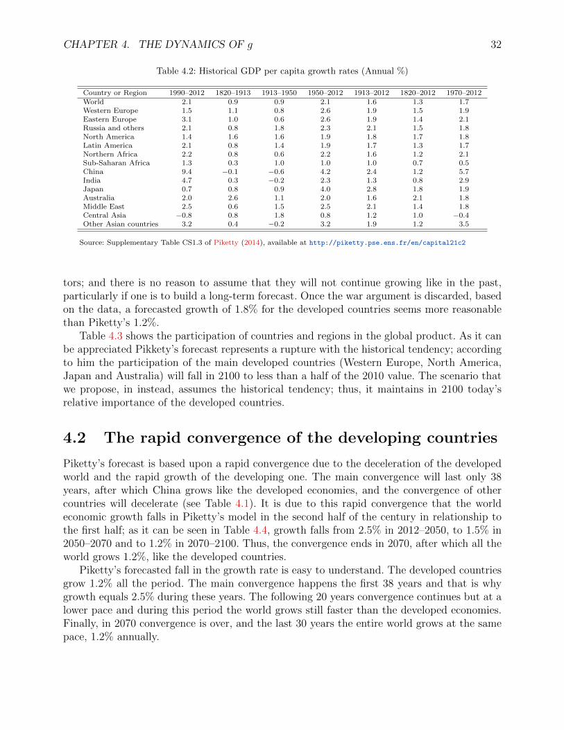
CHAPTER 4. THE DYNAMICS OF g 32
Table 4.2: Historical GDP per capita growth rates (Annual %)
Country or Region 1990–2012 1820–1913 1913–1950 1950–2012 1913–2012 1820–2012 1970–2012World 2.1 0.9 0.9 2.1 1.6 1.3 1.7Western Europe 1.5 1.1 0.8 2.6 1.9 1.5 1.9Eastern Europe 3.1 1.0 0.6 2.6 1.9 1.4 2.1Russia and others 2.1 0.8 1.8 2.3 2.1 1.5 1.8North America 1.4 1.6 1.6 1.9 1.8 1.7 1.8Latin America 2.1 0.8 1.4 1.9 1.7 1.3 1.7Northern Africa 2.2 0.8 0.6 2.2 1.6 1.2 2.1Sub-Saharan Africa 1.3 0.3 1.0 1.0 1.0 0.7 0.5China 9.4 −0.1 −0.6 4.2 2.4 1.2 5.7India 4.7 0.3 −0.2 2.3 1.3 0.8 2.9Japan 0.7 0.8 0.9 4.0 2.8 1.8 1.9Australia 2.0 2.6 1.1 2.0 1.6 2.1 1.8Middle East 2.5 0.6 1.5 2.5 2.1 1.4 1.8Central Asia −0.8 0.8 1.8 0.8 1.2 1.0 −0.4Other Asian countries 3.2 0.4 −0.2 3.2 1.9 1.2 3.5
Source: Supplementary Table CS1.3 of Piketty (2014), available at http://piketty.pse.ens.fr/en/capital21c2
tors; and there is no reason to assume that they will not continue growing like in the past,particularly if one is to build a long-term forecast. Once the war argument is discarded, basedon the data, a forecasted growth of 1.8% for the developed countries seems more reasonablethan Piketty’s 1.2%.
Table 4.3 shows the participation of countries and regions in the global product. As it canbe appreciated Pikkety’s forecast represents a rupture with the historical tendency; accordingto him the participation of the main developed countries (Western Europe, North America,Japan and Australia) will fall in 2100 to less than a half of the 2010 value. The scenario thatwe propose, in instead, assumes the historical tendency; thus, it maintains in 2100 today’srelative importance of the developed countries.
4.2 The rapid convergence of the developing countries
Piketty’s forecast is based upon a rapid convergence due to the deceleration of the developedworld and the rapid growth of the developing one. The main convergence will last only 38years, after which China grows like the developed economies, and the convergence of othercountries will decelerate (see Table 4.1). It is due to this rapid convergence that the worldeconomic growth falls in Piketty’s model in the second half of the century in relationship tothe first half; as it can be seen in Table 4.4, growth falls from 2.5% in 2012–2050, to 1.5% in2050–2070 and to 1.2% in 2070–2100. Thus, the convergence ends in 2070, after which all theworld grows 1.2%, like the developed countries.
Piketty’s forecasted fall in the growth rate is easy to understand. The developed countriesgrow 1.2% all the period. The main convergence happens the first 38 years and that is whygrowth equals 2.5% during these years. The following 20 years convergence continues but at alower pace and during this period the world grows still faster than the developed economies.Finally, in 2070 convergence is over, and the last 30 years the entire world grows at the samepace, 1.2% annually.
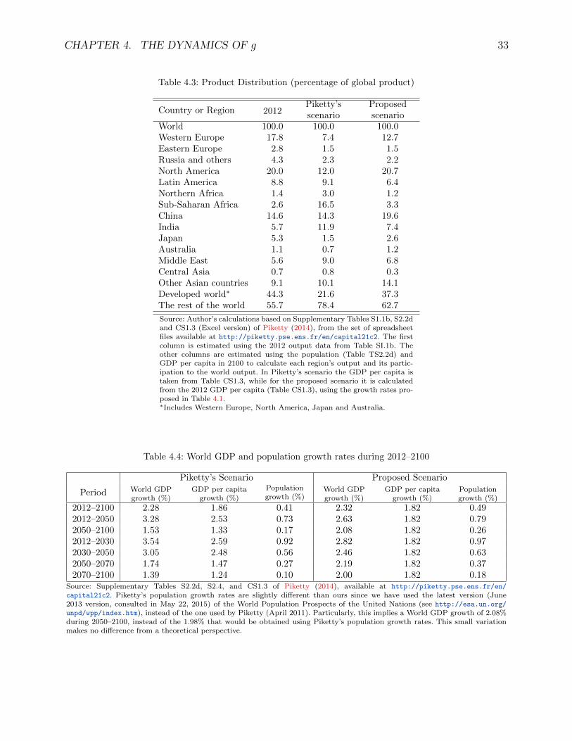
CHAPTER 4. THE DYNAMICS OF g 33
Table 4.3: Product Distribution (percentage of global product)
Country or Region 2012Piketty’sscenario
Proposedscenario
World 100.0 100.0 100.0Western Europe 17.8 7.4 12.7Eastern Europe 2.8 1.5 1.5Russia and others 4.3 2.3 2.2North America 20.0 12.0 20.7Latin America 8.8 9.1 6.4Northern Africa 1.4 3.0 1.2Sub-Saharan Africa 2.6 16.5 3.3China 14.6 14.3 19.6India 5.7 11.9 7.4Japan 5.3 1.5 2.6Australia 1.1 0.7 1.2Middle East 5.6 9.0 6.8Central Asia 0.7 0.8 0.3Other Asian countries 9.1 10.1 14.1Developed world∗ 44.3 21.6 37.3The rest of the world 55.7 78.4 62.7
Source: Author’s calculations based on Supplementary Tables S1.1b, S2.2dand CS1.3 (Excel version) of Piketty (2014), from the set of spreadsheetfiles available at http://piketty.pse.ens.fr/en/capital21c2. The firstcolumn is estimated using the 2012 output data from Table SI.1b. Theother columns are estimated using the population (Table TS2.2d) andGDP per capita in 2100 to calculate each region’s output and its partic-ipation to the world output. In Piketty’s scenario the GDP per capita istaken from Table CS1.3, while for the proposed scenario it is calculatedfrom the 2012 GDP per capita (Table CS1.3), using the growth rates pro-posed in Table 4.1.∗Includes Western Europe, North America, Japan and Australia.
Table 4.4: World GDP and population growth rates during 2012–2100
Piketty’s Scenario Proposed Scenario
Period World GDPgrowth (%)
GDP per capitagrowth (%)
Populationgrowth (%)
World GDPgrowth (%)
GDP per capitagrowth (%)
Populationgrowth (%)
2012–2100 2.28 1.86 0.41 2.32 1.82 0.492012–2050 3.28 2.53 0.73 2.63 1.82 0.792050–2100 1.53 1.33 0.17 2.08 1.82 0.262012–2030 3.54 2.59 0.92 2.82 1.82 0.972030–2050 3.05 2.48 0.56 2.46 1.82 0.632050–2070 1.74 1.47 0.27 2.19 1.82 0.372070–2100 1.39 1.24 0.10 2.00 1.82 0.18
Source: Supplementary Tables S2.2d, S2.4, and CS1.3 of Piketty (2014), available at http://piketty.pse.ens.fr/en/
capital21c2. Piketty’s population growth rates are slightly different than ours since we have used the latest version (June2013 version, consulted in May 22, 2015) of the World Population Prospects of the United Nations (see http://esa.un.org/
unpd/wpp/index.htm), instead of the one used by Piketty (April 2011). Particularly, this implies a World GDP growth of 2.08%during 2050–2100, instead of the 1.98% that would be obtained using Piketty’s population growth rates. This small variationmakes no difference from a theoretical perspective.
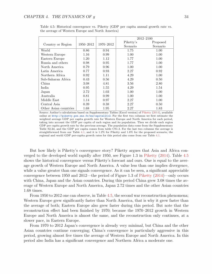
CHAPTER 4. THE DYNAMICS OF g 34
Table 4.5: Historical convergence vs. Piketty (GDP per capita annual growth rate vs.the average of Western Europe and North America)
2012–2100
Country or Region 1950–2012 1970–2012Piketty’sScenario
ProposedScenario
World 0.86 0.94 1.75 1.00Western Europe 1.16 0.99 1.00 1.00Eastern Europe 1.20 1.12 1.77 1.00Russia and others 0.98 0.95 1.77 1.00North America 0.79 0.96 1.00 1.00Latin America 0.77 0.93 2.27 0.92Northern Africa 0.92 1.11 4.29 1.00Sub-Saharan Africa 0.43 0.56 4.29 0.50China 3.08 4.81 3.56 2.80India 0.95 1.55 4.29 1.54Japan 2.72 1.03 1.00 1.00Australia 0.81 0.99 1.00 1.00Middle East 1.14 0.97 2.27 1.00Central Asia 0.39 0.38 2.27 0.50Other Asian countries 1.68 1.95 2.27 1.83
Source: Author’s calculations based on Supplementary Tables (Excel version) of Piketty (2014), availableonline at http://piketty.pse.ens.fr/en/capital21c2. For the first two columns we first estimate theweighted average GDP per capita growth rate for Western Europe and North America for each period,taking into account the GDP per capita of each region and its population. Then we divide each regionGDP per capita growth rate by the previous average. The population data come from the SupplementaryTable S2.2d, and the GDP per capita comes from table CS1.3. For the last two columns the average isstraightforward from our Table 4.1, and it is 1.2% for Piketty and 1.8% for the proposed scenario; theregional and world GDP per-capita growth rates for this period also come from our Table 4.1.
But how likely is Piketty’s convergence story? Piketty argues that Asia and Africa con-verged to the developed world rapidly after 1950, see Figure 1.3 in Piketty (2014). Table 4.5shows the historical convergence versus Piketty’s forecast and ours. One is equal to the aver-age growth of Western Europe and North America. A value less than one implies divergence,while a value greater than one signals convergence. As it can be seen, a significant appreciableconvergence between 1950 and 2012—the period of Figure 1.3 of Piketty (2014)—only occurswith China, Japan and the Asian countries. During this period China grew 3.08 times the av-erage of Western Europe and North America, Japan 2.72 times and the other Asian countries1.68 times.
From 1950 to 2012 one can observe, in Table 4.5, the second war reconstruction phenomena;Western Europe grew significantly faster than North America, that is why it grew faster thanthe average of both; Eastern Europe also grew faster during this period. But note that thereconstruction effect had been finished by 1970; because the 1970–2012 growth in WesternEurope and North America is almost the same, and the reconstruction only continues, at aslower pace, in Eastern Europe.
From 1970 to 2012 Japan’s convergence is already very minimal, but China and the otherAsian countries continue converging; China’s convergence is particularly aggressive in thisperiod, growing almost five times the average of Western Europe and North America. In thisperiod also India has a significant convergence and Northern Africa a moderate one.
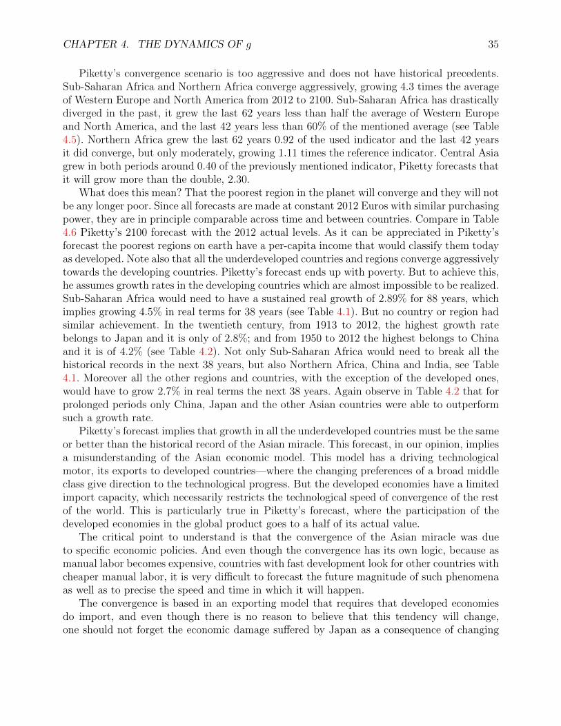
CHAPTER 4. THE DYNAMICS OF g 35
Piketty’s convergence scenario is too aggressive and does not have historical precedents.Sub-Saharan Africa and Northern Africa converge aggressively, growing 4.3 times the averageof Western Europe and North America from 2012 to 2100. Sub-Saharan Africa has drasticallydiverged in the past, it grew the last 62 years less than half the average of Western Europeand North America, and the last 42 years less than 60% of the mentioned average (see Table4.5). Northern Africa grew the last 62 years 0.92 of the used indicator and the last 42 yearsit did converge, but only moderately, growing 1.11 times the reference indicator. Central Asiagrew in both periods around 0.40 of the previously mentioned indicator, Piketty forecasts thatit will grow more than the double, 2.30.
What does this mean? That the poorest region in the planet will converge and they will notbe any longer poor. Since all forecasts are made at constant 2012 Euros with similar purchasingpower, they are in principle comparable across time and between countries. Compare in Table4.6 Piketty’s 2100 forecast with the 2012 actual levels. As it can be appreciated in Piketty’sforecast the poorest regions on earth have a per-capita income that would classify them todayas developed. Note also that all the underdeveloped countries and regions converge aggressivelytowards the developing countries. Piketty’s forecast ends up with poverty. But to achieve this,he assumes growth rates in the developing countries which are almost impossible to be realized.Sub-Saharan Africa would need to have a sustained real growth of 2.89% for 88 years, whichimplies growing 4.5% in real terms for 38 years (see Table 4.1). But no country or region hadsimilar achievement. In the twentieth century, from 1913 to 2012, the highest growth ratebelongs to Japan and it is only of 2.8%; and from 1950 to 2012 the highest belongs to Chinaand it is of 4.2% (see Table 4.2). Not only Sub-Saharan Africa would need to break all thehistorical records in the next 38 years, but also Northern Africa, China and India, see Table4.1. Moreover all the other regions and countries, with the exception of the developed ones,would have to grow 2.7% in real terms the next 38 years. Again observe in Table 4.2 that forprolonged periods only China, Japan and the other Asian countries were able to outperformsuch a growth rate.
Piketty’s forecast implies that growth in all the underdeveloped countries must be the sameor better than the historical record of the Asian miracle. This forecast, in our opinion, impliesa misunderstanding of the Asian economic model. This model has a driving technologicalmotor, its exports to developed countries—where the changing preferences of a broad middleclass give direction to the technological progress. But the developed economies have a limitedimport capacity, which necessarily restricts the technological speed of convergence of the restof the world. This is particularly true in Piketty’s forecast, where the participation of thedeveloped economies in the global product goes to a half of its actual value.
The critical point to understand is that the convergence of the Asian miracle was dueto specific economic policies. And even though the convergence has its own logic, because asmanual labor becomes expensive, countries with fast development look for other countries withcheaper manual labor, it is very difficult to forecast the future magnitude of such phenomenaas well as to precise the speed and time in which it will happen.
The convergence is based in an exporting model that requires that developed economiesdo import, and even though there is no reason to believe that this tendency will change,one should not forget the economic damage suffered by Japan as a consequence of changing
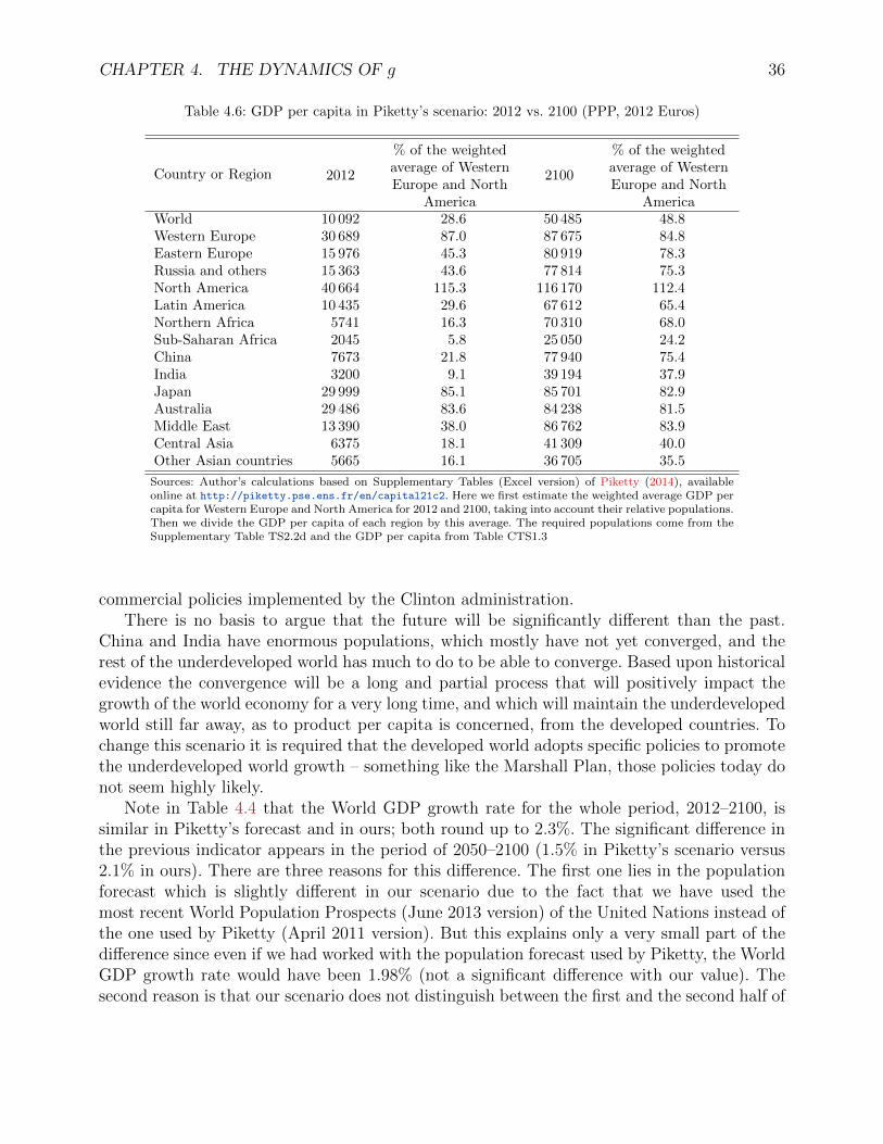
CHAPTER 4. THE DYNAMICS OF g 36
Table 4.6: GDP per capita in Piketty’s scenario: 2012 vs. 2100 (PPP, 2012 Euros)
Country or Region 2012
% of the weightedaverage of WesternEurope and North
America
2100
% of the weightedaverage of WesternEurope and North
AmericaWorld 10 092 28.6 50 485 48.8Western Europe 30 689 87.0 87 675 84.8Eastern Europe 15 976 45.3 80 919 78.3Russia and others 15 363 43.6 77 814 75.3North America 40 664 115.3 116 170 112.4Latin America 10 435 29.6 67 612 65.4Northern Africa 5741 16.3 70 310 68.0Sub-Saharan Africa 2045 5.8 25 050 24.2China 7673 21.8 77 940 75.4India 3200 9.1 39 194 37.9Japan 29 999 85.1 85 701 82.9Australia 29 486 83.6 84 238 81.5Middle East 13 390 38.0 86 762 83.9Central Asia 6375 18.1 41 309 40.0Other Asian countries 5665 16.1 36 705 35.5
Sources: Author’s calculations based on Supplementary Tables (Excel version) of Piketty (2014), availableonline at http://piketty.pse.ens.fr/en/capital21c2. Here we first estimate the weighted average GDP percapita for Western Europe and North America for 2012 and 2100, taking into account their relative populations.Then we divide the GDP per capita of each region by this average. The required populations come from theSupplementary Table TS2.2d and the GDP per capita from Table CTS1.3
commercial policies implemented by the Clinton administration.There is no basis to argue that the future will be significantly different than the past.
China and India have enormous populations, which mostly have not yet converged, and therest of the underdeveloped world has much to do to be able to converge. Based upon historicalevidence the convergence will be a long and partial process that will positively impact thegrowth of the world economy for a very long time, and which will maintain the underdevelopedworld still far away, as to product per capita is concerned, from the developed countries. Tochange this scenario it is required that the developed world adopts specific policies to promotethe underdeveloped world growth – something like the Marshall Plan, those policies today donot seem highly likely.
Note in Table 4.4 that the World GDP growth rate for the whole period, 2012–2100, issimilar in Piketty’s forecast and in ours; both round up to 2.3%. The significant difference inthe previous indicator appears in the period of 2050–2100 (1.5% in Piketty’s scenario versus2.1% in ours). There are three reasons for this difference. The first one lies in the populationforecast which is slightly different in our scenario due to the fact that we have used themost recent World Population Prospects (June 2013 version) of the United Nations instead ofthe one used by Piketty (April 2011 version). But this explains only a very small part of thedifference since even if we had worked with the population forecast used by Piketty, the WorldGDP growth rate would have been 1.98% (not a significant difference with our value). Thesecond reason is that our scenario does not distinguish between the first and the second half of
CHAPTER 4. THE DYNAMICS OF g 37
the twenty-first century, because such a distinction seems, in our opinion, almost impossibleto forecast. The third reason, which is closely related to the previous one, is the regionaldistribution of the product. Contrary to the scenario posed by Piketty, our scenario refusesthe rapid convergence of the underdeveloped countries and maintains the relative importanceof the wealthy countries in the global economy (see Table 4.3).
In particular, observe that in Piketty’s scenario the developed world halves its partici-pation, while Sub-Saharan Africa goes from 2.6% to 16.5%, Northern Africa from 1.4% to3% and India from 5.7% to 11.9%. In our scenario, Western Europe and Japan reduce theirparticipation but less drastically than with Piketty, North America actually increases its par-ticipation slightly. China and the other Asian countries, which with Piketty only maintaintheir participation, will increase it. Sub-Saharan Africa and Northern Africa mostly maintaintheir participation, while India increases it but much less than with Piketty. Eastern Europeand Russia will lose participation, as with Piketty. Latin-America decreases its participationin our scenario, while it increases it with Piketty.
Even though we do not have a real basis to forecast which countries will converge in thetwenty-first century and which ones will not, most likely some will continue converging in thesecond half and some new comers will join. So, it seems that the most probable event is thatthe convergence phenomenon will help sustain a higher growth rate of the global economyfor a long time to come. In particular China, with its enormous population, will take longtime to converge. As social needs increase, the speed of convergence will go down, but it willcontinue for a very long time. In a similar case is India. There are just no reasons to forecastthat the convergence will happen as fast as Piketty has argued. Thus, everything indicatesthat Pikketty’s convergence is way too aggressive.
In summary, the dynamics of g in Piketty’s model mainly depends on two events: 1) theend of the fast technological development which reduces the rate of economic growth of thedeveloped countries, and 2) the end of poverty due to the rapid announced convergence. Bothevents seem to us highly unlikely. An alternative scenario was built in which g for the secondhalf of the twenty-first century is 2.1% versus Piketty’s 1.5%.
Chapter 5
Conclusion
Analyzing together the dynamics of r, s and g, we can build diverse stationary state scenariosfor the second half of the twenty-first century. For g we use two values: Piketty’s 1.5% and the2.1% from the scenario that we propose. For sn we use three values for each g. At g = 1.5% weuse sn = 10% from Piketty; sn = 7.96% coming from a Solow model with sb fixed at its 1990–2010 average value, Table 3.1; and sn = 6.40% coming from Table 3.3 in which we allowed forsb to go down accordingly with the experience in the developed countries. At g = 2.1% we useagain the 10% from Piketty; 9.79% which corresponds to Solow model with fixed sb, Table 3.1;and 8.07% which is the value obtained allowing sb to go down, Table 3.3. For r before taxeswe will take several values: the 4.3% from Piketty and the r that corresponds to each pairformed by the estimated β and the estimate of the gross elasticity of substitution betweencapital and labor: the 0.406 and 0.857 from Chirinko and Mallick (2014), and the 1.25 fromKarabarbounis and Neiman (2014), see Table 2.6. Since there are three estimated β for eachone of the two g’s, and three σgross for each β, we will have a total of eighteen estimated r’s.For the difference between the r before and after taxes we will take three values: 1) the zerotax, t0, in Piketty’s forecast, Table 2.8; 2) capital taxes of 30%, which is the assumption madeby Piketty for the period 1950 to 2012, see the comment below; and 3) capital taxes at 20%.Table 5.1 shows the diverse scenarios.
What is the initial reference? r before taxes for the period 1990–2012 is 4.3%, SupplementalTable S6.2 (Excel version) of Piketty (2014). And the r after taxes for the same period wouldbe 3.01% (4.3%× 0.7); see Piketty (2014) Supplemental Table S10.3. where he uses a tax rateof 0.7 for the period of 1950 to 2012. Piketty also deducts 0.5% due to public firms profitsin the period of 1950–2012 which we are not considering in order to have the same basis ofcomparison going forward. β for 2010 is 440%, Piketty (2014) Supplemental Table S12.4.a.Therefore, using the previous data the reference is: α before taxes of 18.92% (or 440× 0.043),and α after taxes of 13.24% (or 440 × 0.0301). Lets us now discuss. What does Table 5.1 tellus?
In scenarios 1.1 to 6.3 (with R.C denoting the corresponding row and column from Table5.1) r is fixed at 4.3%, Piketty’s assumption. Scenarios 1.4 to 6.12 use an estimated r, whichtakes into account the sensitivity of r in relationship to the value taken by β according todiverse values of σgross (denoted simply as σ hereafter): 0.406, 0.857 and 1.25.
38
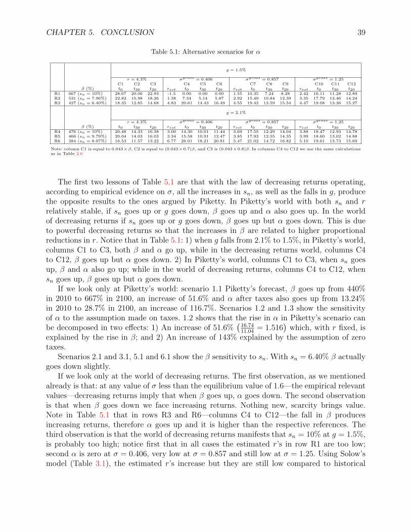
CHAPTER 5. CONCLUSION 39
Table 5.1: Alternative scenarios for α
g = 1.5%
r = 4.3% σgross = 0.406 σgross = 0.857 σgross = 1.25C1 C2 C3 C4 C5 C6 C7 C8 C9 C10 C11 C12
β (%) t0 t30 t20 rest t0 t30 t20 rest t0 t30 t20 rest t0 t30 t20R1 667 (sn = 10%) 28.67 20.06 22.93 -1.5 0.00 0.00 0.00 1.55 10.35 7.24 8.28 2.42 16.11 11.28 12.89R2 531 (sn = 7.96%) 22.82 15.98 18.26 1.38 7.34 5.14 5.87 2.92 15.49 10.84 12.39 3.35 17.79 12.46 14.24R3 427 (sn = 6.40%) 18.35 12.85 14.68 4.83 20.61 14.43 16.49 4.55 19.42 13.59 15.54 4.47 19.08 13.36 15.27
g = 2.1%
r = 4.3% σgross = 0.406 σgross = 0.857 σgross = 1.25β (%) t0 t30 t20 rest t0 t30 t20 rest t0 t30 t20 rest t0 t30 t20
R4 476 (sn = 10%) 20.48 14.33 16.38 3.00 14.30 10.01 11.44 3.69 17.55 12.29 14.04 3.88 18.47 12.93 14.78R5 466 (sn = 9.79%) 20.04 14.03 16.03 3.34 15.58 10.91 12.47 3.85 17.93 12.55 14.35 3.99 18.60 13.02 14.88R6 384 (sn = 8.07%) 16.53 11.57 13.22 6.77 26.01 18.21 20.81 5.47 21.02 14.72 16.82 5.10 19.61 13.73 15.69
Note: column C1 is equal to 0.043×β, C2 is equal to (0.043×0.7)β, and C3 is (0.043×0.8)β. In columns C4 to C12 we use the same calculationsas in Table 2.6
The first two lessons of Table 5.1 are that with the law of decreasing returns operating,according to empirical evidence on σ, all the increases in sn, as well as the falls in g, producethe opposite results to the ones argued by Piketty. In Piketty’s world with both sn and rrelatively stable, if sn goes up or g goes down, β goes up and α also goes up. In the worldof decreasing returns if sn goes up or g goes down, β goes up but α goes down. This is dueto powerful decreasing returns so that the increases in β are related to higher proportionalreductions in r. Notice that in Table 5.1: 1) when g falls from 2.1% to 1.5%, in Piketty’s world,columns C1 to C3, both β and α go up, while in the decreasing returns world, columns C4to C12, β goes up but α goes down. 2) In Piketty’s world, columns C1 to C3, when sn goesup, β and α also go up; while in the world of decreasing returns, columns C4 to C12, whensn goes up, β goes up but α goes down.
If we look only at Piketty’s world: scenario 1.1 Piketty’s forecast, β goes up from 440%in 2010 to 667% in 2100, an increase of 51.6% and α after taxes also goes up from 13.24%in 2010 to 28.7% in 2100, an increase of 116.7%. Scenarios 1.2 and 1.3 show the sensitivityof α to the assumption made on taxes. 1.2 shows that the rise in α in Piketty’s scenario canbe decomposed in two effects: 1) An increase of 51.6%
(16.7411.04
= 1.516)
which, with r fixed, isexplained by the rise in β; and 2) An increase of 143% explained by the assumption of zerotaxes.
Scenarios 2.1 and 3.1, 5.1 and 6.1 show the β sensitivity to sn. With sn = 6.40% β actuallygoes down slightly.
If we look only at the world of decreasing returns. The first observation, as we mentionedalready is that: at any value of σ less than the equilibrium value of 1.6—the empirical relevantvalues—decreasing returns imply that when β goes up, α goes down. The second observationis that when β goes down we face increasing returns. Nothing new, scarcity brings value.Note in Table 5.1 that in rows R3 and R6—columns C4 to C12—the fall in β producesincreasing returns, therefore α goes up and it is higher than the respective references. Thethird observation is that the world of decreasing returns manifests that sn = 10% at g = 1.5%,is probably too high; notice first that in all cases the estimated r’s in row R1 are too low;second α is zero at σ = 0.406, very low at σ = 0.857 and still low at σ = 1.25. Using Solow’smodel (Table 3.1), the estimated r’s increase but they are still low compared to historical

CHAPTER 5. CONCLUSION 40
standards, remember that the average on 1990–2010 was 4.3%, the reason is the increase in βto 531% versus the historical 2010 β of 440%. Using a model that takes into account the fallin sb related to the lower g (Table 3.3), β only falls slightly compared to 2010, and r is alsoslightly higher, in the range of 4.47% to 4.55%. Because β falls it triggers increasing returnsand α goes up but very moderately, in the range 19.08–19.42, versus the initial 18.92. Thefourth observation is that when σ goes up α may go up or down depending on whether β hasincreased or decreased. If β2/β1 > 1, then as σ goes up α goes up. If β2/β1 < 1, then as σ goesup α goes down. But remember that both σ = 0.857 and σ = 1.25 already include the effectof σ going up in the long run. The fifth observation is that there is an interaction between allof the variables, for example compare the scenario 2.10 with 5.10; α is higher in 5.10, despitethe fact that β is lower. The reason is that r is significantly higher in 5.10 due to the lower βas a consequence of the decreasing returns. Also note that β is lower in 5.10 despite the factthat sn is higher; this is consequence of the higher g.
For what we have been arguing Piketty’s forecast has serious difficulties. His main prob-lem is that letting r and sn relatively rigid, he does not take into account the technologicalconstraints of the production function and its consequences in a world where economic agentsoptimize. The outcome is that Piketty’s results are neither theoretically or empirically sat-isfactory. Markets do work, economic agents optimize and the law of decreasing returns ispowerful as the empirical evidence of an σ < 1.25 shows. Not only r goes down proportionallymore to the β increases, but also sb and sn are both a positive function of g.
It is practically impossible to forecast what will happen in the twenty-first century. As wehave been showing, the forecasted results are extremely sensitive to the assumptions made.Moreover, in the real world there may always be speculative waves and price effects. However,long-run forecasts cannot be based in such medium-term distortions that cannot be forecasted.We would like to insist that the most likely long-term forecast is shown in rows R3 and R6,because in them markets are fully operational. These two rows take into account both the lawof decreasing returns and the fact that both sb and sn are a positive function of g. In addition,as to the value of σ, as we argued previously, one should probably be inclined to the rangeof 0.857–1.25, because these values take into account long-term global effects as the marketschange their modes of production. Therefore, it seems that if one is to believe that g will be aslow as Piketty’s forecast (1.5%), then α before taxes will most likely be in the range between19.08 and 19.42; very close to its initial value of 18.92. Whereas, if one believes that g will behigher (2.1%), then α before taxes will be in the range between 19.61 and 21.02. In the otherhand, α after taxes is of course highly sensitive to the tax policy. However, as long as thetax policy remains the same, the results after taxes and before taxes are identical. In Table5.1, with capital taxes at 30%, the level used for building the initial α reference, wheneverα before taxes is higher or lower than the initial reference before taxes, α after taxes is alsohigher or lower than the initial reference after taxes. At g = 1.5%, α after taxes, using thesame row and columns than before, will be in a range between 13.36 and 13.59, again veryclose to its initial reference value of 13.24. At g = 2.1%, α after taxes will be in the range of13.73 to 14.72.
The income distribution between the factors of production, as we always knew, is mostlyrelated to the tax policy. With capital taxes of 20% at g = 1.5% the range for α after taxes
CHAPTER 5. CONCLUSION 41
will be 15.27 to 15.54 and at g = 2.1% the range will be 15.69 to 16.82. Both ranges are notonly higher than the initial reference of 13.74, but also, obviously, higher than the ranges atcapital taxes at 30%, which tell us the importance of the tax policy.
There is not an invisible hand that guarantees that the income distribution amongst thefactors of production will be inherently stable. But neither is there an invisible hand that willdrive capitalism necessarily towards income concentration in favor of the capitalists. Marketsdo work and it is difficult to envision that only due to economic forces the income distributionwill worsen significantly; and in any case, if this were to happen, it would be due to capitalscarcity and not due to capital abundance as Piketty has suggested.
There are powerful medium-term forces that can seriously distort the income distributionamongst the factors of production, like speculative housing waves and other price effects; thereare all sort of institutional factors that may in real life worsen the income distribution; andthere may also be powerful political forces pushing for policies that may deteriorate the incomedistribution (see Acemoglu and Robinson, 2015). Therefore, governments and the society haveto be always alert as to the dynamics of the income distribution in each particular case. But,in the long run the income distribution amongst the factors of production will not, only due toeconomic forces, tend towards the pronounced concentration in favor of capital that Pikettyhas argued.
Epilogue
In this epilogue we briefly make some very general remarks on four topics related to Pikety’sproposal of the general dynamics of capitalism. The first topic is related to the discussionof whether the income distribution is still a good measure of the actual income “enjoyment”by the participants in the economy. The second one has to do with discussing the meaningof income distribution. The third topic is related to the personal income distribution in theWorld Top Incomes Database (WTID). The fourth one is about the dynamics of capitalism.
E.1 Income enjoyment
Piketty’s discussion mainly relates to income distribution and it does not include in a system-atic way the analysis of the consequences of government expenditures. This point is particu-larly crucial in the developed world in which governments control about 40% of the nationalincome, when they only controlled around 10% in the beginning of the twenty-first century.What Piketty has called the patrimonial class is politically and economically significantlybetter at the beginning of the twenty-first century in relationship to the same period in thetwentieth century. Few calculations show that this is the case, but to take this point seriouslyprobably deserves another book of the same size of Piketty’s. The first two columns in TableE.1 show the share of income of the richest decile in the United States, the United Kingdomand France in 1900 and 2010; columns 3 and 4 show the tax revenues of the government on thesame dates; and column five shows the % dedicated to social spending. Table E.2 shows a veryrough calculation on the assumptions that: 1) in 1900 social spending was minimal and totalgovernment expenditures equally affects the richest 10% and the remaining 90%; 2) in 2010 itis assumed that all social spending goes to the less rich 90% and that the non-social spendingequally affects the richest 10% and the remaining 90%. The results are the outcome of a veryrough calculation but they are striking. In the United States, despite the fact that the 10%has 47.9% of national income in 2010, versus 40.5% in 1900, once government expendituresare introduced, the 10% enjoys only 34% in 2010 versus 38% in 1900. In the U.K., the 10% has41.6% of the income in 2010 versus 47.1% in 1900; and the 10% enjoys only 26% of the incomein 2010 versus 44% in 1900. In France the 10% has 33% of the income in 2010 versus 45.5%in 1900; and the 10% enjoys only 18% in 2010 versus 43% in 1900. This rough calculationclearly shows the point that we wanted to illustrate. Democracy, in the developed economies,has implied that the less rich 90% of the population has gained significant command on theenjoyment of national income.
42
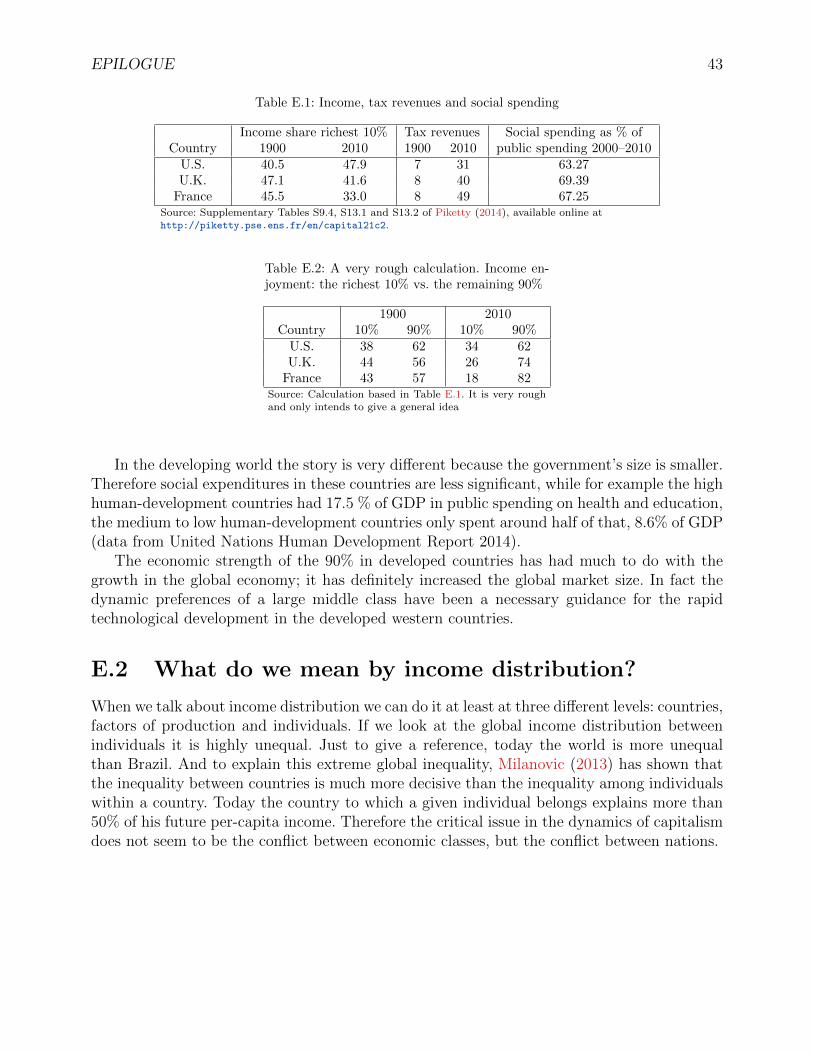
EPILOGUE 43
Table E.1: Income, tax revenues and social spending
Income share richest 10% Tax revenues Social spending as % ofCountry 1900 2010 1900 2010 public spending 2000–2010
U.S. 40.5 47.9 7 31 63.27U.K. 47.1 41.6 8 40 69.39
France 45.5 33.0 8 49 67.25Source: Supplementary Tables S9.4, S13.1 and S13.2 of Piketty (2014), available online athttp://piketty.pse.ens.fr/en/capital21c2.
Table E.2: A very rough calculation. Income en-joyment: the richest 10% vs. the remaining 90%
1900 2010Country 10% 90% 10% 90%
U.S. 38 62 34 62U.K. 44 56 26 74
France 43 57 18 82Source: Calculation based in Table E.1. It is very roughand only intends to give a general idea
In the developing world the story is very different because the government’s size is smaller.Therefore social expenditures in these countries are less significant, while for example the highhuman-development countries had 17.5 % of GDP in public spending on health and education,the medium to low human-development countries only spent around half of that, 8.6% of GDP(data from United Nations Human Development Report 2014).
The economic strength of the 90% in developed countries has had much to do with thegrowth in the global economy; it has definitely increased the global market size. In fact thedynamic preferences of a large middle class have been a necessary guidance for the rapidtechnological development in the developed western countries.
E.2 What do we mean by income distribution?
When we talk about income distribution we can do it at least at three different levels: countries,factors of production and individuals. If we look at the global income distribution betweenindividuals it is highly unequal. Just to give a reference, today the world is more unequalthan Brazil. And to explain this extreme global inequality, Milanovic (2013) has shown thatthe inequality between countries is much more decisive than the inequality among individualswithin a country. Today the country to which a given individual belongs explains more than50% of his future per-capita income. Therefore the critical issue in the dynamics of capitalismdoes not seem to be the conflict between economic classes, but the conflict between nations.
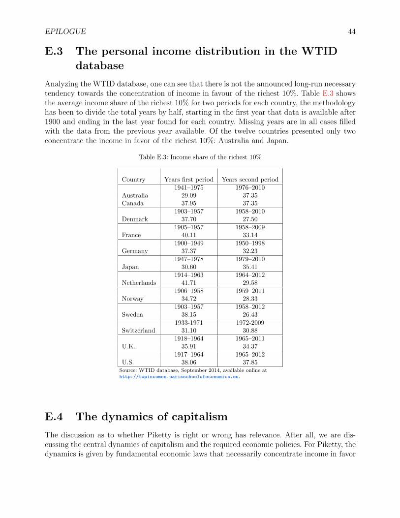
EPILOGUE 44
E.3 The personal income distribution in the WTID
database
Analyzing the WTID database, one can see that there is not the announced long-run necessarytendency towards the concentration of income in favour of the richest 10%. Table E.3 showsthe average income share of the richest 10% for two periods for each country, the methodologyhas been to divide the total years by half, starting in the first year that data is available after1900 and ending in the last year found for each country. Missing years are in all cases filledwith the data from the previous year available. Of the twelve countries presented only twoconcentrate the income in favor of the richest 10%: Australia and Japan.
Table E.3: Income share of the richest 10%
Country Years first period Years second period1941–1975 1976–2010
Australia 29.09 37.35Canada 37.95 37.35
1903–1957 1958–2010Denmark 37.70 27.50
1905–1957 1958–2009France 40.11 33.14
1900–1949 1950–1998Germany 37.37 32.23
1947–1978 1979–2010Japan 30.60 35.41
1914–1963 1964–2012Netherlands 41.71 29.58
1906–1958 1959–2011Norway 34.72 28.33
1903–1957 1958–2012Sweden 38.15 26.43
1933-1971 1972-2009Switzerland 31.10 30.88
1918–1964 1965–2011U.K. 35.91 34.37
1917–1964 1965–2012U.S. 38.06 37.85
Source: WTID database, September 2014, available online athttp://topincomes.parisschoolofeconomics.eu.
E.4 The dynamics of capitalism
The discussion as to whether Piketty is right or wrong has relevance. After all, we are dis-cussing the central dynamics of capitalism and the required economic policies. For Piketty, thedynamics is given by fundamental economic laws that necessarily concentrate income in favor
EPILOGUE 45
of the capitalists, laws that have to be opposed by the institutions. Thus, there is in Pikettyan inherent economic conflict between the most privileged and the rest of the population.Moreover, with his convergence mechanism he gets rid of the unequal income distributionbetween countries. As we have been discussing he is wrong. The main conflict to be resolved,as far as income distribution is concerned, is between nations, not between classes. The worldhas a lot to gain if the developed countries seriously commit themselves to the growth of thedeveloping ones.
In the developed countries there is a clear triumph of the masses as to the size of theeconomic resources that they enjoy. And the rapid development of the middle class in thesecountries has been a motor engine for the growth of the whole world. The growing middles classhas enlarged the market to unprecedented levels; and the dynamic process of their changingpreferences has lead to technological change in the west—this was the crucial difference withRussia for example. It must be remarked, that the growing middle class in the west not onlyexplains the rapid development of this region, but it has also been the key in the success of theAsian miracle whose economic model is based upon exports to the middle class in the west.One of the key problems in the developing economies is that they do not have the requiredmiddle class size.
Piketty emphasizes a groundless economic dynamics—one which necessarily implies classconflict—and he undermines the two crucial factors that have characterized global capitalism:the rapid growth of the middle class in developed countries and the lasting highly unequaldistribution between countries.

Bibliography
Daron Acemoglu and James A. Robinson. The Rise and Decline of General Laws of Capital-ism. Journal of Economic Perspectives, 29(1):3–28, 2015. URL http://www.aeaweb.org/
articles.php?doi=10.1257/jep.29.1.3.
Odran Bonnet, Pierre-Henri Bono, Guillaume Chapelle, and Etienne Wasmer. Does hous-ing capital contribute to inequality? A comment on Thomas Piketty’s Capital in the21st Century. Sciences Po Economics Discussion Papers 2014-07, Sciences Po De-partement of Economics, July 2014. URL http://spire.sciencespo.fr/hdl:/2441/
30nstiku669glbr66l6n7mc2oq/.
Robert S. Chirinko and Debdulal Mallick. The Substitution Elasticity, Factor Shares, Long-Run Growth, and the Low-Frequency Panel Model. CESifo Working Paper Series 4895,CESifo Group Munich, October 2014. URL http://papers.ssrn.com/sol3/papers.cfm?
abstract_id=2479816.
Charles I. Jones. The Shape of Production Functions and the Direction of TechnicalChange. The Quarterly Journal of Economics, 120(2):517–549, 2005. URL http://qje.
oxfordjournals.org/content/120/2/517.abstract.
Loukas Karabarbounis and Brent Neiman. The Global Decline of the Labor Share. TheQuarterly Journal of Economics, 129(1):61–103, 2014. URL http://qje.oxfordjournals.
org/content/129/1/61.abstract.
Per Krusell and Antony A. Smith. Is Piketty’s “Second law of Capitalism” Fundamental?,May 2015. URL http://aida.wss.yale.edu/smith/piketty1.pdf. (to be published).
Debdulal Mallick. The Role of the Elasticity of Substitution in Economic Growth: A Cross-Country Test of the de La Grandville Hypothesis. Economics Series 4, Deakin University,Faculty of Business and Law, School of Accounting, Economics and Finance, May 2007. URLhttp://www.deakin.edu.au/buslaw/aef/workingpapers/papers/2007_04eco.pdf.
Debdulal Mallick. The role of the elasticity of substitution in economic growth: A cross-countryinvestigation. Labour Economics, 19(5):682–694, 2012. URL http://www.sciencedirect.
com/science/article/pii/S0927537112000310.
46
BIBLIOGRAPHY 47
Branko Milanovic. Global Income Inequality in Numbers: in History and Now. Global Pol-icy, 4(2):198–208, 2013. ISSN 1758-5899. URL http://dx.doi.org/10.1111/1758-5899.
12032.
Ezra Oberfield and Devesh Raval. Micro Data and Macro Technology. NBER Working Papers20452, National Bureau of Economic Research, September 2014. URL http://www.nber.
org/papers/w20452.
Thomas Piketty. Capital in the Twenty-First century. Harvard University Press, April 2014.
Thomas Piketty and Gabriel Zucman. Capital is Back: Wealth-Income Ratios in Rich Coun-tries 1700–2010. The Quarterly Journal of Economics, 129(3):1255–1310, 2014. URLhttp://qje.oxfordjournals.org/content/129/3/1255.abstract.
Matthew Rognlie. A note on Piketty and diminishing returns to capital, June 2014. URLhttp://www.mit.edu/~mrognlie/piketty_diminishing_returns.pdf.
Robert M. Solow. Thomas Piketty Is Right: Everything you need to know about ‘Capitalin the Twenty-First Century’, April 2014. URL http://www.newrepublic.com/article/
117429/.