alvaredo garbinti piketty - hceo · piketty and zucman (2014), atkinson (2014), ohlsson, roine and...
TRANSCRIPT

On the long run evolution of inherited wealth
The United States in historical and comparative
perspectives 1880-2010
Facundo Alvaredo Nuffield College-EMod, PSE & Conicet
Bertrand Garbinti
CREST-INSEE & PSE
Thomas Piketty Paris School of Economics
HCEO Conference on Social Mobility Chicago, November 4-5, 2014

• What do we know about the historical patterns of inheritance in the US?
• Main goal: to provide estimates of the share of inherited wealth in aggregate wealth (φ=WB/W) in the US over 1880-2010 [1860-2013]
• There seemed to be a general presumption that φ=WB/W should decrease over time, perhaps due to the rise in human capital (leading to the rise of the labor share in income and savings), and/or the rise of lifecycle wealth accumulation
• Only recently there has been new evidence for FR, UK, SWE, GER, …
• For the US, the 1980s Kotlikoff-Summers-Modigliani controversy:
Modigliani: WB/W as little as 20-30%
Kotlikoff-Summers: WB/W is as high as 80-90%
They were looking at the same data!
• For the US, Wolff and Gittleman (2013): WB/W dropped from 29% to 19% over 1989-2007

Piketty and Zucman (2014), Atkinson (2014), Ohlsson, Roine and Waldenstrom (2013), and Schinke (2013)
The inheritance share in aggregate wealth accumulation follows a U-shaped curve in France and Germany, and to a more limited extent in the UK. It follows a broadly similar pattern in Sweden, although in recent decades the Swedish inheritance stock increased relatively little, as the private saving rate increased. It is likely that gifts are under-estimated in the UK at the end of the period.
20%
30%
40%
50%
60%
70%
80%
90%
100%
1880 1900 1920 1940 1960 1980 2000
The stock of inherited wealth / private wealth φ =WB/W in Europe 1880-2010
France UK Germany Sweden
0%
4%
8%
12%
16%
20%
24%
1900 1910 1920 1930 1940 1950 1960 1970 1980 1990 2000 2010
Annu
al fl
ow o
f beq
uest
s an
d gi
fts (%
nat
iona
l inco
me)
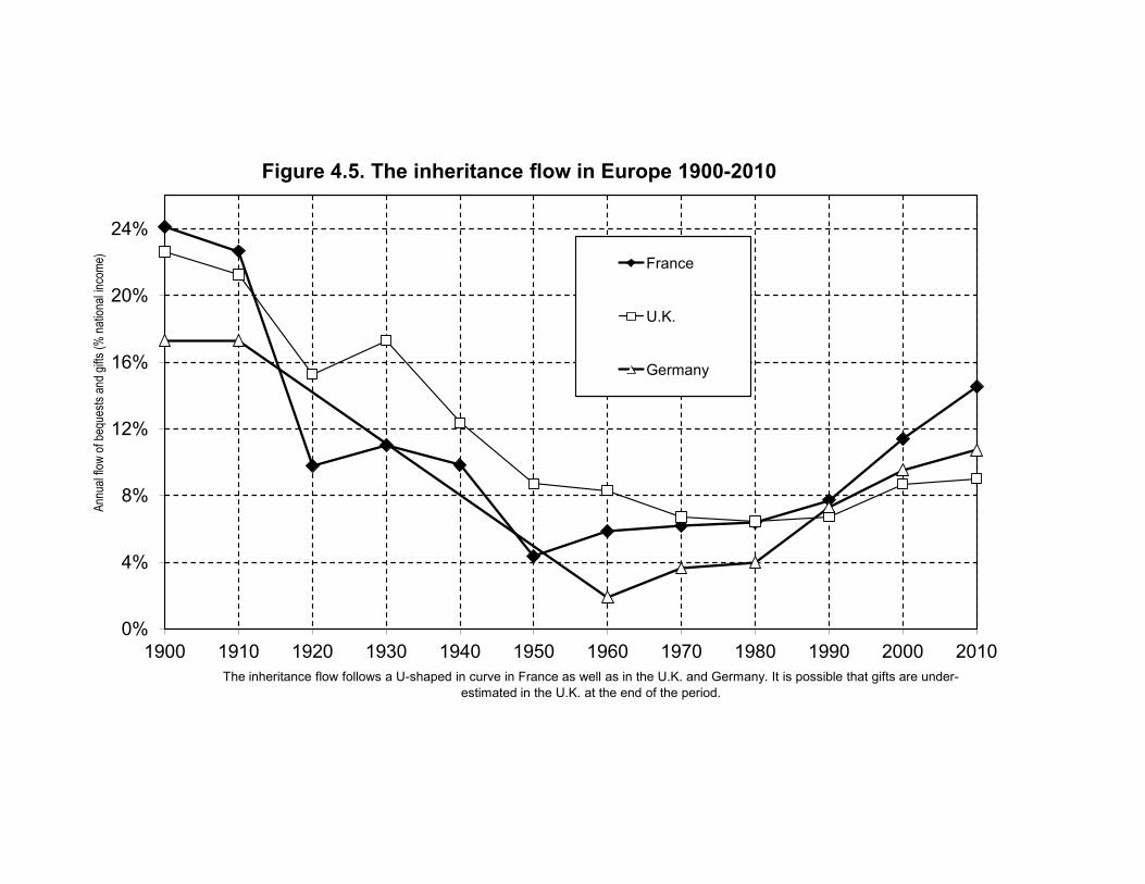
The inheritance flow follows a U-shaped in curve in France as well as in the U.K. and Germany. It is possible that gifts are under-estimated in the U.K. at the end of the period.
Figure 4.5. The inheritance flow in Europe 1900-2010
France
U.K.
Germany

Outline • This is an area where available evidence is scarce and incomplete.
• It is also an area where it is important to be particularly careful about concepts and definitions.
1. Basic notions and definitions
2. The Kotlikoff-Summers-Modigliani controversy and the
capitalization factor
3. The Piketty-Postel Vinay-Rosenthal definition (PPVR)
4. A simplified definition: inheritance flows vs. saving flows
5. Evidence
6. Discussion

1. Basic notions and definitions • We would like to estimate the share of inherited wealth in total wealth φ=WB/W
• It might seem natural to define WBt as the sum of past inheritance flows:
• Several problems arise when applied to actual data
o It is critical to include inter-vivos gift flows
o Only consider bequests received by individuals still alive in t
where vt is an estimate of the gift/bequest ratio
4 The long-run evolution of the share of inherited wealth
4.1 Concepts, data sources and methods
We now turn to our third ratio of interest, the share of inherited wealth in aggregate wealth.
We should make clear at the outset that this is an area where available evidence is scarce
and incomplete. Measuring the share of inherited wealth requires a lot more data than the
measurement of aggregate wealth-income ratios or even wealth concentration. It is also an
area where it is important to be be particularly careful about concepts and definitions. Purely
definitional conflicts have caused substantial confusion in the past. Therefore it it critical to
start from there.
4.1.1 Basic notions and definitions
The most natural way to define the share of inherited wealth in aggregate wealth is to cumulate
past inheritance flows. That is, assume that we observe the aggregate wealth stock Wt at time
t in a given country, and that we would like to define and estimate the aggregate inherited
wealth stock WBt Wt (and conversely aggregate self-made wealth, which we simply define as
WSt = Wt �WBt). Assume that we observe the annual flow of inheritance Bs that occured in
any year s t. At first sight, it might seem natural to define the stock of inherited wealth WBt
as the sum of past inheritance flows:
WBt =
Z
st
Bs · ds
However, there are several practical and conceptual di�culties with this ambiguous defini-
tion, which need to be addressed before the formula can be applied to actual data. First, it is
critical to include in this sum not only past bequest flows Bs (wealth transmissions at death)
but also inter vivos gift flows Vs (wealth transmissions inter vivos). That is, one should define
WBt as WBt =R
st
B⇤s · ds., with B⇤
s = Bs + Vs.
Alternatively, if one cannot observe directly the gift flow Vs, one should replace the observed
bequest flow Bs by some grossed up level B⇤s = (1 + vs) · Bs, where vs = Vs/Bs is an estimate
of the gift/bequest flow ratio. In countries where adequate data is available, the gift/bequest
ratio is at least 10-20%, and is often higher than 50%, especially in the recent period.20 It is
20See below. Usually one only includes formal, monetary capital gifts, and one ignores informal presents and
18
thus critical to include gifts in one way or another. In countries where fiscal data on gifts is
insu�cient, one should at least try to estimate a gross-up factor 1+vs using surveys (which often
su↵ers from severe downward biases) and harder administrative evidence from other countries.
Next, in order to properly apply this definition, one should only take into account the fraction
of the aggregate inheritance flow Bst Bs that was received at time s by individuals who are
still alive at time t. The problem is that doing so properly requires very detailed individual-level
information. At any time t, there are always individuals who received inheritance a very long
time ago (say, 60 years ago) but who are still alive (because they inherited at a very young age
and/or are enjoying a very long life). Conversely, a fraction of the inheritance flow received
a short time ago (say, 10 years ago) should not be counted (because the relevant inheritors
are already dead, e.g., they inherited at an old age or died young). In practice, however, such
unusual events tend to balance each other, so that a standard simplifying assumption is to
cumulate the full inheritance flows observed the previous H years, where H is the average
generation length, i.e. the average age at which parents have children (typically H = 30 years).
Therefore we obtain the following simplified definition:
WBt =
Z
t�30st
(1 + vs) · Bs · ds
4.1.2 The Kotliko↵-Summers-Modigliani controversy
Assume now that these two di�culties can be addressed (i.e., that we can properly estimate
the gross up factor 1 + vs and the average generation length H). There are more substantial
di�culties ahead. First, in order to properly compute WBt, one needs to be able to observe
inheritance flows B⇤s over a relatively long time period (typically, the previous 30 years). In
the famous Kotliko↵-Summers-Modigliani (KSM) controversy, both Kotliko↵-Summers (1981,
1988) and Modigliani (1986, 1988) used estimates of the US inheritance flow for only one year
(and a relatively ancient year: 1962). They simply assumed that this estimate could be used for
other years. Namely, they assumed that the inheritance flow-national income ratio (which we
note bys = B⇤s/Ys) is stable over time. One problem with this assumption is that it might not
be verified. As we shall see below, extensive historical data on inheritances recently collected
in-kind gifts. In particular in-kind gifts made to minors living with their parents (i.e. the fact that minor childrenare usually catered by their parents) are generally left aside.
19

2. The Kotlikoff-Summers-Modigliani controversy • One needs to observe inheritance flows over a relatively long period of time (eg H=30 years)
• Kotlikoff-Summers (1981, 1988) and Modigliani (1986, 1988) used the US inheritance flow by=By/Y for one year (1962), and assumed that it was stable over time. [!]
• -One needs to decide on the capitalization rate
Modigliani Kotlikoff-Summers Capitalization
rate 0 average rate of return to wealth
φt=WBt/Wt
g=r=0 then for ß=400%
and by=10% both definitions coincide:
75% r-g=2%
then for ß=400% and by=10%
56% 103%
Results for US 20-30% 80-90%
in France show that the bys ratio has changed tremendously over the past two centuries, from
about 20-25% of national income in the 19th and early 20th centuries, down to less than 5% at
mid-20th century, back to about 15% in the early 21st century (Piketty, 2011). So one cannot
simply use one year of data and assume that we are in a steady-state: one needs long-run time
series on the inheritance flow in order to estimate the aggregate stock of inherited wealth.
Next, one needs to decide the extent to which past inheritance flows need to be upgraded
or capitalized. This is the main source of disagreement and confusion in the KSM controversy.
Modigliani (1986, 1988) chooses zero capitalization. That is, he simply defines the stock of
inherited wealth WMBt as the raw sum of past inheritance flows with no adjustment whatsoever
(except for the GDP price index):
WMBt =
Z
t�30st
B⇤s · ds
Assume a fixed inheritance flow-national income ratio by = B⇤s/Ys, growth rate g (so that
Yt = Ys · eg(t�s)), generation length H, and aggregate private wealth-national income ratio
� = Wt/Yt. Then, according to the Modigliani definition, the steady-state formulas for the
stock of inherited wealth relative to national income WMBt/Yt and for the share of inherited
wealth 'Mt = WM
Bt/Wt are given by:
WMBt/Yt =
1
Yt
Z
t�30st
B⇤s · ds =
1� e�gH
g· by
'Mt = WM
Bt/Wt =1� e�gH
g· by�
In contrast, Kotliko↵ and Summers (1981, 1988) choose to capitalize past inheritance flows
by using the economy’s average rate of return to wealth (assuming it is constant and equal
to r). Following the Kotliko↵-Summers definition, the steady-state formulas for the stock of
inherited wealth relative to national income WKSBt /Yt and for the share of inherited wealth
'KSt = WKS
Bt /Wt are given by:
WKSBt /Yt =
1
Yt
Z
t�30st
er(t�s) · B⇤s · ds =
e(r�g)H � 1
r � g· by
'KSt = WKS
Bt /Wt =e(r�g)H � 1
r � g· by�
20
In the special case where growth rates and rates of return are negligible (i.e., infinitely close
to zero), then both definitions coincide. That is, if g = 0 and r � g = 0, then (1 � e�gH)/g =
(e(r�g)H � 1)/(r � g) = H , so that WMBt/Yt = WKS
Bt /Yt = Hby and 'Mt = 'KS
t = Hby/�.
Thus, in case growth and capitalization e↵ects can be neglected, one simply needs to multiply
the annual inheritance flow by generation length. If the annual inheritance flow is equal to
by = 10% of national income, and generation length is equal to H = 30 years, then the stock
of inherited wealth is equal to WMBt = WKS
Bt = 300% of national income according to both
definitions. In case aggregate wealth amounts to � = 400% of national income, then the
inheritance share is equal to 'Mt = 'KS
t = 75% of aggregate wealth.
However, in the general case where g and r � g are significantly di↵erent from zero, the
two definitions can lead to widely di↵erent conclusions. For instance, with g = 2%, r = 4%
and H = 30, we have the following capitalization factors: (1 � e�gH)/(g · H) = 0.75 and
(e(r�g)H � 1)/((r � g) ·H) = 1.37. In this example, for a given inheritance flow by = 10% and
aggregate wealth-income ratio � = 400%, we obtain 'Mt = 56% and 'KS
t = 103%. About half
of wealth comes from inheritance according to the Modigiani definition, and all of it according
to the Kotliko↵-Summers definition.
This is the main reason why Modigliani and Kotliko↵-Summers disagree so much about the
inheritance share. They both use the same (relatively fragile) estimate for the US by in 1962.
But Modigliani does not capitalize past inheritance flows and concludes that the inheritance
share is as low as 20-30%. Kotliko↵-Summers do capitalize the same flows and conclude that
the inheritance share is as large as 80-90% (or even larger than 100%). Both sides also disagree
somewhat about the measurement of by, but the main source of disagreement comes from this
capitalization e↵ect.21
4.1.3 The limitations of KSM definitions
Which of the two definitions is most justified? In our view, both are problematic. It is wholly
inappropriate not to capitalize at all past inheritance flows. But full capitalization is also
inadequate.
The key problem with the KSM representative-agent approach is that it fails to recognize
21In e↵ect, Modigliani favors a by ratio around 5-6%, while Kotliko↵-Summers find it more realistic to use a byratio around 7-8%. Given the data sources they use, it is likely that both sides tend to somewhat underestimatethe true ratio. See below the discussion for the case of France and other European countries.
21

3. The Piketty-Postel Vinay-Rosenthal (PPVR) definition
• Both no-capitalization and full capitalization seem inadequate
• In an ideal world with perfect data, we would like to observe:
o (a) inheritors: their assets are worth less than the capitalized value of the wealth they inherited (they consume more than their labor income)
o (b) savers/self-made individuals: their assets are worth more than the capitalized value of the wealth they inherited (they consume less than their labor income)
• So aggregate inherited wealth=inheritors’ wealth + inherited fraction of savers’
wealth
• Self-made wealth: non-inherited fraction of savers’ wealth
Straightforward definition, but very demanding in terms of data. It requires good quality micro-data over generations. However, no need to observe yt , ct paths.
and savers; wrt = E(wti|wti < b⇤ti) and ws
t = E(wti|wti � b⇤ti) the average wealth levels of both
groups; br⇤t = E(b⇤ti|wti < b⇤ti) and bs⇤t = E(b⇤ti|wti � b⇤ti) the levels of their average capitalized
bequest; and ⇡t = ⇢t · wrt /wt and 1� ⇡t = (1� ⇢t) · ws
t/wt the share of inheritors and savers in
aggregate wealth.
We define the total share 't of inherited wealth in aggregate wealth as the sum of inheritors’
wealth plus the inherited fraction of savers’ wealth, and the share 1�'t of self-made wealth as
the non-inherited fraction of savers’ wealth:
't = [⇢t · wrt + (1� ⇢t) · bs⇤t ]/wt = ⇡t + (1� ⇢t) · bs⇤t /wt
1� 't = (1� ⇢t) · (wst � bs⇤t )/wt = 1� ⇡t � (1� ⇢t) · bs⇤t /wt
The downside of this definition is that it is more demanding in terms of data availability.
While Modigliani and Kotliko↵-Summers could compute inheritance shares in aggregate wealth
by using aggregate data only, the PPVR definition requires micro data. Namely, we need data
on the joint distribution Gt(wti, b⇤ti) of current wealth wti and capitalized inherited wealth b⇤ti
in order to compute ⇢t, ⇡t and 't. This does require high-quality, individual-level data on
wealth and inheritance over two generations, which is often di�cult to obtain. It is worth
stressing, however, that we do not need to know anything about the individual labor income or
consumption paths (yLsi, csi, s < t) followed by individual i up to the time of observation.23
For plausible joint distributions Gt(wti, b⇤ti), the PPVR inheritance share 't will typically
fall somewhere in the interval ['Mt ,'KS
t ]. There is, however, no theoretical reason why it should
be so in general. Imagine for instance an economy where inheritors consume their bequests the
very day they receive it, and never save afterwards, so that wealth accumulation entirely comes
from the savers, who never received any bequest (or negligible amounts), and who patiently
accumulate savings from their labor income. Then with our definition 't = 0%: in this economy,
100% of wealth accumulation comes from savings, and nothing at all comes from inheritance.
23Of course more data are better. If we also have (or estimate) labor income or consumption paths, then onecan compute lifetime individual savings rate sBti, i.e. the share of lifetime resources that was not consumed upto time t: sBti = wti/(b⇤ti+ y⇤Lti) = 1� c⇤ti/(b
⇤ti+ y⇤Lti), with y⇤Lti =
Rs<t
yLsier(t�s)ds = capitalized value at time t
of past labor income flows, and c⇤ti =R
s<tcsie
r(t�s)ds = capitalized value at time t of past consumption flows.By
definition, inheritors are individuals who consumed more than their labor income (i.e. wti < b⇤ti $ c⇤ti > y⇤Lti),while savers are individuals who consumed less than their labor income (i.e. wti � b⇤ti $ c⇤ti y⇤Lti). But thepoint is that we only need to observe an individual’s wealth (wti) and capitalized inheritance (b⇤ti) in order todetermine whether he or she is an inheritor or a saver, and in order to compute the share of inherited wealth.
24

4. A simplified definition: inheritance flow vs. saving flow
• Assume that all we have is macro data:
• We want to estimate φ=WB/W
We do not know which part of the saving rate come from returns to inherited wealth and which comes from labor earnings or past savings
• Assume the propensity to save is the same on both income sources:
o a fraction φα of the saving is attributed to the returns of inherited wealth
o a fraction (1-α)+(1-φ)α is attributed to labor income and past savings
• relatively lower saving rates imply larger φ
However with the Modigliani and Kotliko↵-Summers definitions, the inheritance shares 'Mt and
'KSt could be arbitrarily large.
4.1.5 A simplified definition: inheritance flows vs. saving flows
When available micro data is not su�cient to apply the PPVR definition, one can also use a
simplified, approximate definition based upon the comparison between inheritance flows and
saving flows.
Assume that all we have is macro data on inheritance flows byt = Bt/Yt and savings flows
st = St/Yt. Suppose for simplicity that both flows are constant over time: byt = by and st = s.
We want to estimate the share ' = WB/W of inherited wealth in aggregate wealth. The
di�culty is that we typically do not know which part of the aggregate saving rate s comes the
return to inherited wealth, and which part comes from labor income (or from the return to
past savings). Ideally, one would like to distinguish between the savings of inheritors and savers
(defined along the lines defined above), but this requires micro data over two generations. In
the absence of such data, a natural starting point would be to assume that the propensity to
save is on average the same whatever the income sources. That is, a fraction ' ·↵ of the saving
rate s should be attributed to the return to inherited wealth, and a fraction 1� ↵+ (1� ') · ↵
should be attributed to labor income (and to the return to past savings), where ↵ = YK/Y is
the capital share in national income and 1 � ↵ = YL/Y is the labor share. Assuming again
that we are in steady-state, we obtain the following simplified formula for the share of inherited
wealth in aggregate wealth:
' =by + ' · ↵ · s
by + s
I.e., ' =by
by + (1� ↵) · sIntuitively, this formula simply compares the size of the inheritance and saving flows. Since
all wealth must originate from one of the two flows, it is the most natural way to estimate the
share of inherited wealth in total wealth.24
24Similar formulas based upon the comparison of inheritance and saving flows have been used by De Long(2003) and Davies et al (2012, p.123-124). One important di↵erence is that these authors do not take intoaccount the fact that the saving flow partly comes from the return to inherited wealth. We return to this pointin section 5.4 below.
25

4. A simplified definition for φ (cont.)
• Caveats o Real economies are generally out of steady state, so compute average
(eg H=30 years)
o This is an approximate formula. It tends to underestimate the true share of
inheritance if individuals who only have labor income save less than those with large inherited wealth
• However o It follows micro-based estimates relatively closely o It is much less demanding in terms of data o It does not depend explicitly on the rate of return
There are a number of caveats with this simplified formula. First, real-world economies are
generally out of steady-state, so it is important to compute average values of by, s and ↵ over
relatively long periods of time (typically over the past H years, with H = 30 years). If one has
time-series estimates of the inheritance flow bys, capital share ↵s and saving rate ss then one
can use the following full formula, which capitalizes past inheritance and savings flows at rate
r � g:
' =
R
t�Hst
e(r�g)(t�s) · bys · dsR
t�Hst
e(r�g)(t�s) · (bys + (1� ↵s) · ss) · ds
With constant flows, the full formula boils down to ' =by
by + (1� ↵) · s .
Second, one should bear in mind that the simplified formula ' = by/(by + (1� ↵) · s) is an
approximate formula. In general, as we show below, it tends to under-estimate the true share
of inheritance, as computed from micro data using the PPVR definition. The reason is that
individuals who only have labor income tend to save less (in proportion to their total income)
than those who have large inherited wealth and capital income, which in turns seems to be
related to the fact that wealth (and particularly inherited wealth) is more concentrated than
labor income.
On the positive side, simplified estimates of ' seem to follow micro-based estimates relatively
closely (much more closely than KSM estimates, which are either far too small or far too large),
and they are much less demanding in terms of data. One only needs to estimate macro flows.
Another key advantage of the simplified definition over KSM definitions is that it does not
depend upon the sensitive choice of the rate of return or the rate of capital gains or losses.
Whatever these rates might be, they should apply equally to inherited and self-made wealth (at
least as a first approximation), so one can simply compare inheritance and saving flows.
4.2 The long-run evolution of inheritance in France 1820-2010
4.2.1 The inheritance flow-national income ratio byt
What do we empirically know about the historical evolution of inheritance? We start by pre-
senting the evidence on the dynamics of the inheritance to national income ratio byt in France,
a country for which, as we have seen in section 3, historical data sources are exceptionally good
(Piketty, 2011). The main conclusion is that byt has followed a spectacular U-shaped pattern
26
20%
30%
40%
50%
60%
70%
80%
90%
100%
1850 1870 1890 1910 1930 1950 1970 1990 2010
Cum
ulat
ed s
tock
of i
nher
ited
weal
th (%
priv
ate
weal
th)
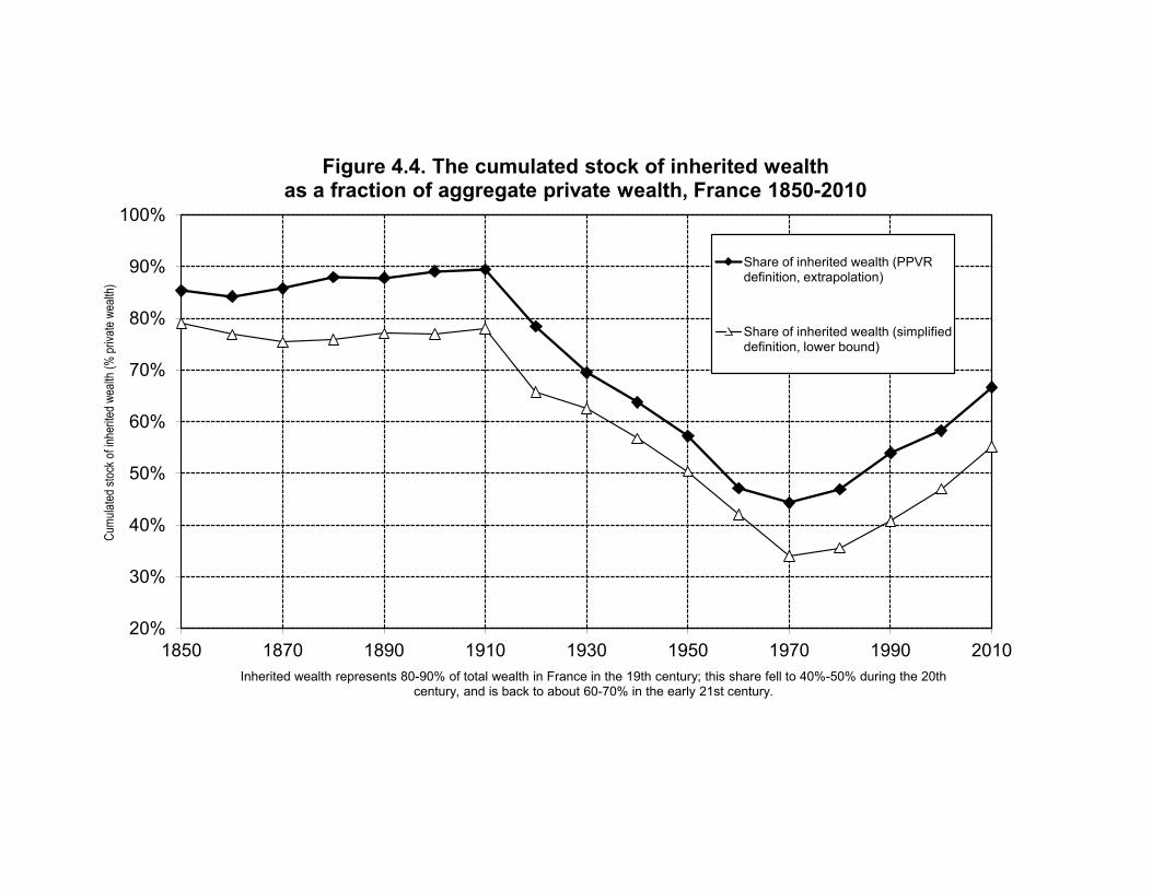
Inherited wealth represents 80-90% of total wealth in France in the 19th century; this share fell to 40%-50% during the 20th century, and is back to about 60-70% in the early 21st century.
Figure 4.4. The cumulated stock of inherited wealth as a fraction of aggregate private wealth, France 1850-2010
Share of inherited wealth (PPVR definition, extrapolation)
Share of inherited wealth (simplified definition, lower bound)
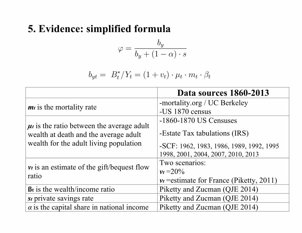
5. Evidence: simplified formula
Data sources 1860-2013 mt is the mortality rate
-mortality.org / UC Berkeley -US 1870 census
µt is the ratio between the average adult wealth at death and the average adult wealth for the adult living population
-1860-1870 US Censuses
-Estate Tax tabulations (IRS)
-SCF: 1962, 1983, 1986, 1989, 1992, 1995 1998, 2001, 2004, 2007, 2010, 2013
vt is an estimate of the gift/bequest flow ratio
Two scenarios: vt =20% vt =estimate for France (Piketty, 2011)
ßt is the wealth/income ratio Piketty and Zucman (QJE 2014) st private savings rate Piketty and Zucman (QJE 2014) α is the capital share in national income Piketty and Zucman (QJE 2014)
However with the Modigliani and Kotliko↵-Summers definitions, the inheritance shares 'Mt and
'KSt could be arbitrarily large.
4.1.5 A simplified definition: inheritance flows vs. saving flows
When available micro data is not su�cient to apply the PPVR definition, one can also use a
simplified, approximate definition based upon the comparison between inheritance flows and
saving flows.
Assume that all we have is macro data on inheritance flows byt = Bt/Yt and savings flows
st = St/Yt. Suppose for simplicity that both flows are constant over time: byt = by and st = s.
We want to estimate the share ' = WB/W of inherited wealth in aggregate wealth. The
di�culty is that we typically do not know which part of the aggregate saving rate s comes the
return to inherited wealth, and which part comes from labor income (or from the return to
past savings). Ideally, one would like to distinguish between the savings of inheritors and savers
(defined along the lines defined above), but this requires micro data over two generations. In
the absence of such data, a natural starting point would be to assume that the propensity to
save is on average the same whatever the income sources. That is, a fraction ' ·↵ of the saving
rate s should be attributed to the return to inherited wealth, and a fraction 1� ↵+ (1� ') · ↵
should be attributed to labor income (and to the return to past savings), where ↵ = YK/Y is
the capital share in national income and 1 � ↵ = YL/Y is the labor share. Assuming again
that we are in steady-state, we obtain the following simplified formula for the share of inherited
wealth in aggregate wealth:
' =by + ' · ↵ · s
by + s
I.e., ' =by
by + (1� ↵) · sIntuitively, this formula simply compares the size of the inheritance and saving flows. Since
all wealth must originate from one of the two flows, it is the most natural way to estimate the
share of inherited wealth in total wealth.24
24Similar formulas based upon the comparison of inheritance and saving flows have been used by De Long(2003) and Davies et al (2012, p.123-124). One important di↵erence is that these authors do not take intoaccount the fact that the saving flow partly comes from the return to inherited wealth. We return to this pointin section 5.4 below.
25
over the 20th century. The inheritance flow was relatively stable around 20–25% of national
income throughout the 1820–1910 period (with a slight upward trend), before being divided by
a factor of about 5–6 between 1910 and the 1950s, and then multiplied by a factor of about 3–4
between the 1950s and the 2000s (see figure 4.1).
These are enormous historical variations, but they appear to be well founded empirically.
In particular, the patterns for byt are similar with two independent measures of the inheritance
flow. The first, what we call the fiscal flow, uses bequest and gift tax data and makes allowances
for tax-exempt assets such as life insurance. The second measure, what we call the economic
flow, combines estimates of private wealth Wt, mortality tables and observed age-wealth profile,
using the following accounting equation:
B⇤t = (1 + vt) · µt ·mt ·Wt
Where: mt = mortality rate (number of adult decedents divided by total adult population)
µt = ratio between average adult wealth at death and average adult wealth for the entire
population
vt = Vt/Bt = estimate of the gift/bequest flow ratio
The gap between the fiscal and economic flows can be interpreted as capturing tax evasion
and other measurement errors. It is approximately constant over time and relatively small, so
that the two series deliver consistent long-run patterns (see figure 4.1).
The economic flow series allow – by construction – for a straightforward decomposition of
the various e↵ects at play in the evolution of byt. In the above equation, dividing both terms
by Yt we get:
byt = B⇤t /Yt = (1 + vt) · µt ·mt · �t
Similarly, dividing by Wt we can define the rate of wealth transmission bwt:
bwt = B⇤t /Wt = (1 + vt) · µt ·mt = µ⇤
t ·mt
with µ⇤t = (1 + vt) · µt = gift-corrected ratio
If µt = 1 (i.e., decedents have the same average wealth as the living) and vt = 0 (no gift),
then the rate of wealth transmission is simply equal to the mortality rate: bwt = mt (and
byt = mt · �t). If µt = 0 (i.e., decedents die with zero wealth, like in Modigliani’s pure life-cycle
27

0%
5%
10%
15%
20%
25%
30%
1860 1880 1900 1920 1940 1960 1980 2000
The annual inheritance flow as a fraction of national income by=B/Y
byt = µt mt βt with vt=20% byt = µt mt βt with vt for France byt = µt mt βt for France
100%
200%
300%
400%
500%
600%
700%
800%
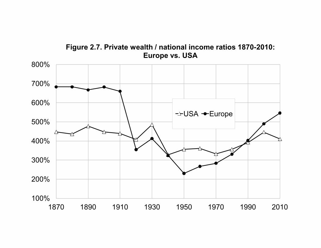
1870 1890 1910 1930 1950 1970 1990 2010 Private wealth = non-financial assets + financial assets - financial liabilities (household & non-profit sectors). Data are decennial
averages (1910-1913 averages for Europe)
Figure 2.7. Private wealth / national income ratios 1870-2010: Europe vs. USA
USA Europe

20%
30%
40%
50%
60%
70%
80%
90%
100%
1880 1900 1920 1940 1960 1980 2000
The stock of inherited wealth / private wealth φ =WB/W in the US 1880-2010
US with vt=20% US with vt=France

Piketty and Zucman (2014), Atkinson (2014), Ohlsson, Roine and Waldenstrom (2013), and Schinke (2013)
The inheritance share in aggregate wealth accumulation follows a U-shaped curve in France and Germany, and to a more limited extent in the UK. It follows a broadly similar pattern in Sweden, although in recent decades the Swedish inheritance stock increased relatively little, as the private saving rate increased. It is likely that gifts are under-estimated in the UK at the end of the period.
20%
30%
40%
50%
60%
70%
80%
90%
100%
1880 1900 1920 1940 1960 1980 2000
The stock of inherited wealth / private wealth φ =WB/W in Europe and the US 1880-2010
France UK Germany Sweden US

5. Evidence: PPVR formula
SCF: 1962, 1983, 1986, 1989, 1992, 1995 1998, 2001, 2004, 2007, 2010, 2013
and savers; wrt = E(wti|wti < b⇤ti) and ws
t = E(wti|wti � b⇤ti) the average wealth levels of both
groups; br⇤t = E(b⇤ti|wti < b⇤ti) and bs⇤t = E(b⇤ti|wti � b⇤ti) the levels of their average capitalized
bequest; and ⇡t = ⇢t · wrt /wt and 1� ⇡t = (1� ⇢t) · ws
t/wt the share of inheritors and savers in
aggregate wealth.
We define the total share 't of inherited wealth in aggregate wealth as the sum of inheritors’
wealth plus the inherited fraction of savers’ wealth, and the share 1�'t of self-made wealth as
the non-inherited fraction of savers’ wealth:
't = [⇢t · wrt + (1� ⇢t) · bs⇤t ]/wt = ⇡t + (1� ⇢t) · bs⇤t /wt
1� 't = (1� ⇢t) · (wst � bs⇤t )/wt = 1� ⇡t � (1� ⇢t) · bs⇤t /wt
The downside of this definition is that it is more demanding in terms of data availability.
While Modigliani and Kotliko↵-Summers could compute inheritance shares in aggregate wealth
by using aggregate data only, the PPVR definition requires micro data. Namely, we need data
on the joint distribution Gt(wti, b⇤ti) of current wealth wti and capitalized inherited wealth b⇤ti
in order to compute ⇢t, ⇡t and 't. This does require high-quality, individual-level data on
wealth and inheritance over two generations, which is often di�cult to obtain. It is worth
stressing, however, that we do not need to know anything about the individual labor income or
consumption paths (yLsi, csi, s < t) followed by individual i up to the time of observation.23
For plausible joint distributions Gt(wti, b⇤ti), the PPVR inheritance share 't will typically
fall somewhere in the interval ['Mt ,'KS
t ]. There is, however, no theoretical reason why it should
be so in general. Imagine for instance an economy where inheritors consume their bequests the
very day they receive it, and never save afterwards, so that wealth accumulation entirely comes
from the savers, who never received any bequest (or negligible amounts), and who patiently
accumulate savings from their labor income. Then with our definition 't = 0%: in this economy,
100% of wealth accumulation comes from savings, and nothing at all comes from inheritance.
23Of course more data are better. If we also have (or estimate) labor income or consumption paths, then onecan compute lifetime individual savings rate sBti, i.e. the share of lifetime resources that was not consumed upto time t: sBti = wti/(b⇤ti+ y⇤Lti) = 1� c⇤ti/(b
⇤ti+ y⇤Lti), with y⇤Lti =
Rs<t
yLsier(t�s)ds = capitalized value at time t
of past labor income flows, and c⇤ti =R
s<tcsie
r(t�s)ds = capitalized value at time t of past consumption flows.By
definition, inheritors are individuals who consumed more than their labor income (i.e. wti < b⇤ti $ c⇤ti > y⇤Lti),while savers are individuals who consumed less than their labor income (i.e. wti � b⇤ti $ c⇤ti y⇤Lti). But thepoint is that we only need to observe an individual’s wealth (wti) and capitalized inheritance (b⇤ti) in order todetermine whether he or she is an inheritor or a saver, and in order to compute the share of inherited wealth.
24
100%
150%
200%
250%
300%
350%
400%
450%
500%
550%
1989 1992 1995 1998 2001 2004 2007 2010 2013
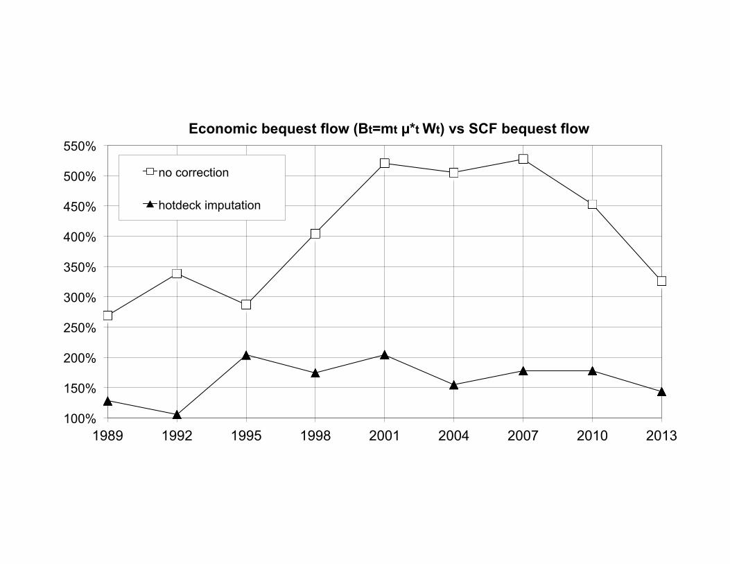
Economic bequest flow (Bt=mt µ*t Wt) vs SCF bequest flow
no correction
hotdeck imputation

0%
10%
20%
30%
40%
50%
60%
70%
80%
90%
100%
1989 1991 1993 1995 1997 1999 2001 2003 2005 2007 2009 2011 2013
The stock of inherited wealth / private wealth φ =WB/W in the US 1989-2013
simplified formula (vt=20%) simplified formula (vt=France) SCF-original SCF-correction=4 SCF-hotdeck imputation
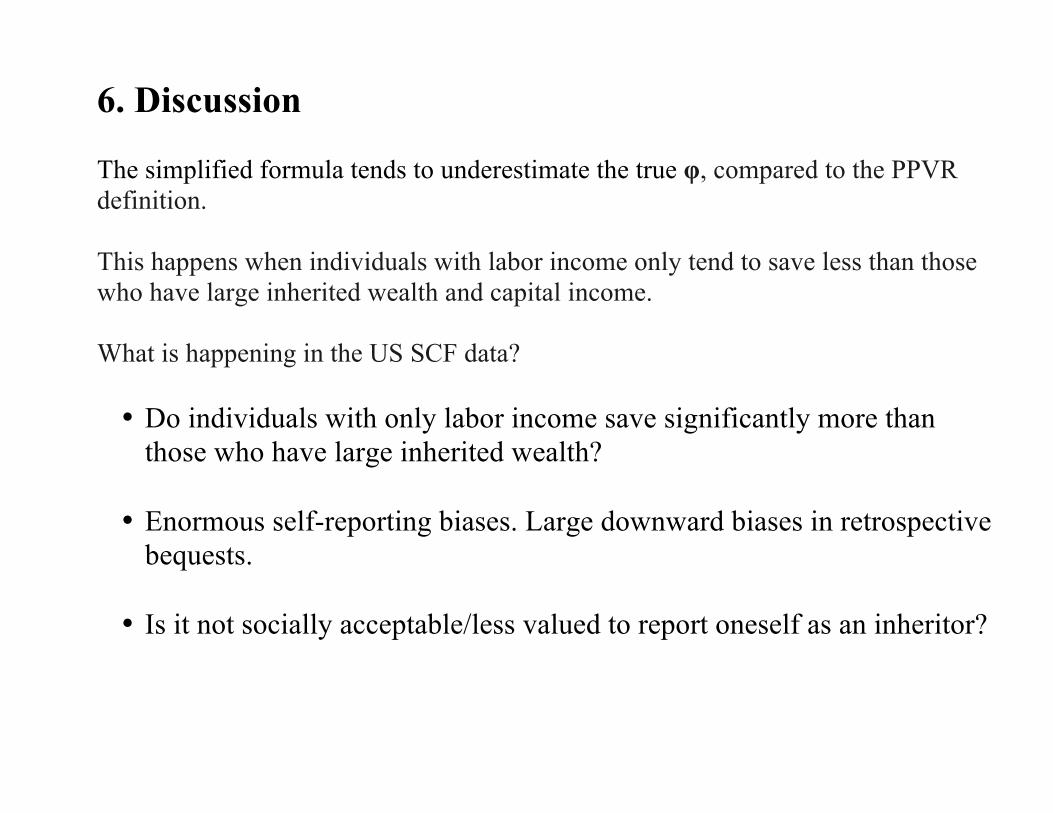
6. Discussion The simplified formula tends to underestimate the true φ, compared to the PPVR definition. This happens when individuals with labor income only tend to save less than those who have large inherited wealth and capital income. What is happening in the US SCF data? • Do individuals with only labor income save significantly more than
those who have large inherited wealth?
• Enormous self-reporting biases. Large downward biases in retrospective bequests.
• Is it not socially acceptable/less valued to report oneself as an inheritor?

