HAL Id: hal-00769225https://hal.inria.fr/hal-00769225

Submitted on 30 Dec 2012

HAL is a multi-disciplinary open accessarchive for the deposit and dissemination of sci-entific research documents, whether they are pub-lished or not. The documents may come fromteaching and research institutions in France orabroad, or from public or private research centers.

L’archive ouverte pluridisciplinaire HAL, estdestinée au dépôt et à la diffusion de documentsscientifiques de niveau recherche, publiés ou non,émanant des établissements d’enseignement et derecherche français ou étrangers, des laboratoirespublics ou privés.

Pigasus : Python for IsoGeometric AnalysiS and UnifiedSimulations.Ahmed Ratnani

To cite this version:Ahmed Ratnani. Pigasus : Python for IsoGeometric AnalysiS and Unified Simulations.. [TechnicalReport] 2012. hal-00769225

Πgasus : Python for IsoGeometric AnalysiS and UnifiedSimulations

Ahmed RATNANI 1

1C.E.A./DSM/IRFM, Cadarache, FRahmed.ratnani@cea.fr

Abstract

B-splines and NURBS (Non Uniform Rational B-splines) are widely used in CAD (ComputerAider Design) models. IGA (IsoGeometric Analysis) consists of using these functions to both de-fine the geometry and represent the unknowns that are solution of a Partial Differential Equation,using the Finite Element principle. In this paper we present a new library, namely Πgasus , thatwas developped in order to bring a common framework between the users (especially physicists)and mathematicians. We want to provide a stable and robust framework, that handles complexgeometries and models as it is the case in Plasma Physics. Physicists will be able to use the recentworks and results obtained by mathematicians. Πgasus is a 1D, 2D and 3D Fortran code, inter-faced with Python. It provides a Geometry module, a FEM (Finite Element Method) computationalengine and a Visualization module.

1 Introduction

The IsoGeometric Analysis has been introduced by Hughes et al [32], in order to bring a commonframework between CAD (Computer Aided Design) and Numerical Simulations. During the wholeprocess, including refinement and analysis, the geometry is maintained exact. In addition to theclassical refinement strategies, hp-refinement, IGA introduces a new one, namelly the k-refinement. Thelatter offers the possiblity to control the regularity of the basis functions, by increasing or decreasingthe multiplicities of knots. From this point of view, IGA can be seen as a generalization of standardFEMs where more regular functions are used.

In addition to handle complex and CAD geometries, it has been shown [18] that, the use of regularelements reduces the dimension of the Finite Element spaces, while keeping the desired precision. Itallows to deal with higher order differential operators [25]. Moreover, it has been noticed [45], thatthe use of regular elements tends to give better CFL numbers.

For a comprehensive introduction on the subject, we may refeer the reader to the recent book byCottrel et al [13]. For an algorithmic overview on B-splines we refeer to the book by DeBoor [20] orPiegl and Tiller [40]. For an extensive overview on the approximation theory, we may suggest thebooks [21, 50].

IGA is getting a large success inside the Engineering and Mathematical communities. The in-creasing number of publications shows the interest of these communities to this new approach. It hasbeen used in electromagnetism [11, 10, 45], in incompressible fluid dynamics [9], in fluid-structureinteraction [29, 6] or using a mapped Finite Volume method [26], in structural and contact mechanics[53, 33]. IGA has been used in Plasmas Physics, in MHD (Magneto-HydroDynamics) problems [46],and the Kinetic approach [14, 1, 4].

1

An active area of research is the study of local refinement. It seems that T-splines are getting morepopular. Many studies are under investigation to understand the behavior of the discrete spaces[7, 17] or to glue 2 patchs [16], which is of a big importance for parallelization.

Another active area is how to construct a volume description of a computational domain, givenby its boundary, so we can directly use all existing CAD-models. For those interested in this subject,we may refeer to the works [35, 36, 37, 12, 59, 60].

Some useful softwares can be found ([57], [19]) to accompany researchers and introduce themto this new subject. However, for real and complex applications, they present some disadvantages.They are inflexible for Numerical Simulations combined with Modeling. In the latter, the user maywant to see the effect of adding a new term, or remove it, test a new time scheme, etc .... In order tosolve partial differential equations (PDEs), one needs to copy the old written code, and then change it.Hence, we will end up with as many as codes, as the problems we have treated, even if the principalchanges occure while assembling the element matrices.

All these points, motivated me to developp a new library, Πgasus , written in Fortran and inter-faced with Python. The idea was to simplify as much as possible this interface, so we can recoverthe classical language of the Finite Element Method, while maintaining the advantages of a scripted-language. By sharing the library between different projects, we will keep the same computationalengine, and so reduce redundancy. In addition, the architecture of Πgasus offers the user the abilityto manipulate the geometry and refine it (using the hpk-refinement strategies), use high order and reg-ular elements, and to manipulate the differential operators even for non-linear problems. The designof Πgasus gives the user some freedom to define the spaces and manipulate the grids (thus relax theisoparametric approach, by considering edge, surface, . . . elements).

Πgasus is not intend (for the moment) to be a concurrent of automated FEM softwares likeFreefem++ or Feelpp [41, 28].

This work was motivated by the increasing interactions between physicists and mathematiciansin (computational) plasma physics, trying to answer the question : how can a mathematician studyand improve physicists works and challenges, and make his developpements promptly available? Itwas initiated during my Phd-thesis [44] at the INRIA, and pursued at the CEA. We wanted to provideboth physicists and mathematicians a common framework where they can developp their researchs,take advantage from the IGA approach, but also in the future for production cases.

As the reader will notice it, the user does not need to have a deep knowledge on CAD or B-splines. The important point is to know how to derive a variational (weak) formulation, and thenask Πgasus to assemble the different parts of the formulation. Πgasus is delivered with a (2D)simple and easy GUI interface to create and manipulate the computational domains. The user canmove and manipulate the control points in order to generate the geometry. The basic distribution ofΠgasus does not need any third package or library.

Throughout this article, we will present 2D studies even if the code treats also the 1D and 3Dcases. The current paper is structured as follows. In section 2, we give a brief overview on B-splines,NURBS and IsoGeometric Analysis approach. In section 3, we present Πgasus on a simple example(Poisson’s equation). We have made an effort to link each of Πgasus ’s functions to the FEM language.In section 4, we give much more details on Πgasus : its architecture, the important concepts, utilitiesand features. Finally, in section 5, we a non-linear 2D pde as a simple application. This article is nota tutorial, but we have tried to present as mush as possible the different and interesting parts.

2 An overview on IsoGeometric Analysis

More details on the subject can be found in [21, 50, 40, 20, 13].

2

2.1 Basic properties of B-splines

Definition 2.1 (B-Spline) Let X = x0, · · · , xp a non-decreasing sequence of p+ 1 points such that x0 6=xp. The B-Spline is defined by the following reccurence formula:

N(x;x0, · · · , xp) =x− x0

xp−1 − x0N(x;x0, · · · , xp−1) +

xp − xxp − x1

N(x;x1, · · · , xp) (2.1)

the initialization is given by : N(x;x0, x1) = 1, if x0 6= x1, and 0 otherwise.

In order to construct a B-spline of degree p, we need p+1 points which are called knots in the splineterminology. Then, to create a family of B-splines, we will need to have a non-decreasing sequence ofknots, also called knot vector.

Let T = (ti)16i6N+k be a non-decreasing sequence of knots, with k = p+ 1. Each set of p+ 1 con-secutive knots Tj = tj , · · · , tj+pwill generate a B-spline Nj . This leads to the following definition:

Definition 2.2 (B-Spline series) The j-th B-Spline of order k is defined by the recurrence relation:

Nkj = wkjN

k−1j + (1− wkj+1)Nk−1

j+1

where,wkj (x) =

x− tjtj+k−1 − tj

N1j (x) = χ[tj ,tj+1[(x)

for k ≥ 1 and 1 ≤ j ≤ N .

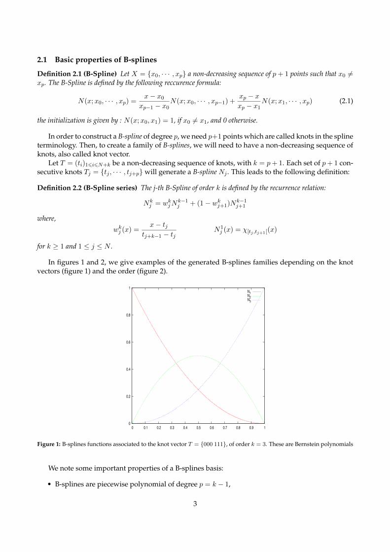
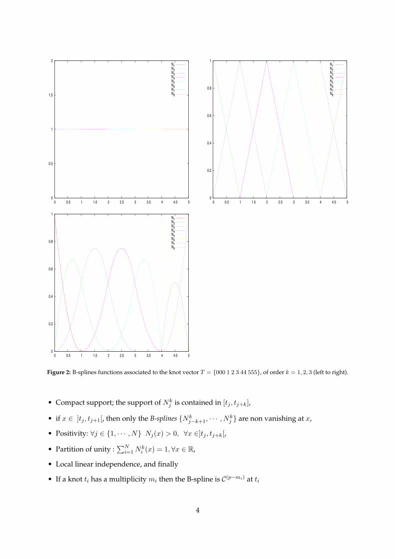
In figures 1 and 2, we give examples of the generated B-splines families depending on the knotvectors (figure 1) and the order (figure 2).

0

0.2

0.4

0.6

0.8

1

0 0.1 0.2 0.3 0.4 0.5 0.6 0.7 0.8 0.9 1

N1N2N3

Figure 1: B-splines functions associated to the knot vector T = 000 111, of order k = 3. These are Bernstein polynomials

We note some important properties of a B-splines basis:

• B-splines are piecewise polynomial of degree p = k − 1,

3

0

0.5

1

1.5

2

0 0.5 1 1.5 2 2.5 3 3.5 4 4.5 5

N1N2N3N4N5N6N7N8

0

0.2

0.4

0.6

0.8

1

0 0.5 1 1.5 2 2.5 3 3.5 4 4.5 5

N1N2N3N4N5N6N7N8

0

0.2

0.4

0.6

0.8

1

0 0.5 1 1.5 2 2.5 3 3.5 4 4.5 5

N1N2N3N4N5N6N7N8

Figure 2: B-splines functions associated to the knot vector T = 000 1 2 3 44 555, of order k = 1, 2, 3 (left to right).

• Compact support; the support of Nkj is contained in [tj , tj+k],

• if x ∈ ]tj , tj+1[, then only the B-splines Nkj−k+1, · · · , Nk

j are non vanishing at x,

• Positivity: ∀j ∈ 1, · · · , N Nj(x) > 0, ∀x ∈]tj , tj+k[,

• Partition of unity :∑N

i=1Nki (x) = 1,∀x ∈ R,

• Local linear independence, and finally

• If a knot ti has a multiplicity mi then the B-spline is C(p−mi) at ti

4

2.2 Multivariate tensor product splines

Let us consider d knot vectors T = T 1, T 2, · · · , T d. For simplicity, we consider that those knotvectors are open, which means that k knots on each side are duplicated so that the spline is interpo-lating on the boundary, and of bounds 0 and 1. In the sequel we will use the notation I = [0, 1]. Eachknot vector T i, will generate a basis for a Schoenberg space [21], Ski(T i, I). The tensor product ofall those spaces is also a Schoenberg space, namely Sk(T ), where k = k1, · · · , kd. The hypercubeP = Id = [0, 1]d, will be referred to as a patch.The basis for Sk(T ) is defined by a tensor product :

Nki := Nk1

i1⊗Nk2

i2⊗ · · · ⊗Nkd

id

where, i = i1, · · · , id.A typical cell from P is a cube of the form : Qi = [ξi1 , ξi1+1]⊗ · · · ⊗ [ξid , ξid+1]. To any cell Q, we willassociate its extension Q, which is the union of the supports of basis functions, that intersects Q.

2.3 Splines in CAD

In order to have a control on the regularity of the curve, we need to use a piecewise-polynomialform. This is why the use of B-splines has known a large success. Moreover, the control points (andpolygone) have many geometric interpretations.Let (Pi)16i6N ∈ Rd be a sequence of control points, forming a control polygon.

Definition 2.3 (B-Spline curve) The B-spline curve in Rd associated to T = (ti)16i6N+k and (Pi)16i6N isdefined by :

C(t) =N∑i=1

Nki (t)Pi

We have the following properties for a B-spline curve:

• If N = k, then C is just a Bezier-curve,

• C is a piecewise polynomial curve,

• The curve interpolates its extremas if the associated multiplicity of the first and the last knotare maximum (i.e. equal to k),

• Invariance with respect to affine transformations,

• Strong convex-hull property:

if ti ≤ t ≤ ti+1, then C(t) is inside the convex-hull associated to the control points Pi−p, · · · ,Pi,

• Local modification : moving Pi affects C(t), only in the interval [ti, ti+k],

• The control polygon approaches the behavior of the curve.

Remark 2.4 Remark that there is a kind of duality between knots and control points. We can use multiplecontrol points : Pi = Pi+1, instead of multiple knots.

5

Deriving a B-spline curve: We have:

C′(t) =n∑i=1

Nki′(t)Pi =

n∑i=1

(p

ti+p − tiNk−1i (t)Pi −

p

ti+1+p − ti+1Nk−1i+1 (t)Pi

)=

n−1∑i=1

Nk−1i

∗(t)Qi

(2.2)where Qi = p Pi+1−Pi

ti+1+p−ti+1, and Nk−1

i

∗, 1 ≤ i ≤ n− 1 are generated using the knot vector T ∗ which

is obtained from T by reducing by one the multiplicity of the first and the last knot (in the case ofopen knot vector), i.e. by removing the first and the last knot.

Example: T = 000 25

35 111, p = 2, n = 5.

We have C(t) =∑5

i=1N3i′(t)Pi, then

C′(t) =4∑i=1

N2i∗(t)Qi

whereQ1 = 5P2 −P1, Q2 =

10

3P3 −P2,

Q3 =10

3P4 −P3, Q4 = 5P5 −P4.

The B-splines N2i∗, 1 ≤ i ≤ 4 are associated to the knot vector T ∗ = 00 2

535 11.

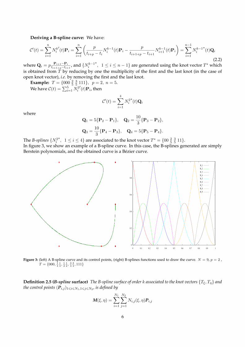
In figure 3, we show an example of a B-spline curve. In this case, the B-splines generated are simplyBerstein polynomials, and the obtained curve is a Bezier curve.

Figure 3: (left) A B-spline curve and its control points, (right) B-splines functions used to draw the curve. N = 9, p = 2 ,T = 000, 1

414, 12

12, 34

34, 111

Definition 2.5 (B-spline surface) The B-spline surface of order k associated to the knot vectors Tξ, Tη andthe control points (Pi,j)16i6N1,16j6N2 , is defined by

M(ξ, η) =

N1∑i=1

N2∑j=1

Ni,j(ξ, η)Pi,j

6

with Ni,j(ξ, η) = N(1)i (ξ)N

(2)j (η)

2.4 Fundamental geometric operations

We can change the curve’s parameters without changing the curve. This refers as to geometric op-erations. For example, we can elevate the spline’s degree or insert new knots. Many algorithms areavailable from the CAD community, and have proved their efficiency [20, 38, 30, 42, 34].In figure 4, we show the use of some of these geometric operations (elevation degree and knot in-sertion) on a quadratic B-Spline curve. We show also how one can split a domain by raising themultiplicity of knots to the spline’s degree. This is an important strategy that may help us for do-main decomposition and parallelization.In figure 5, we show the use of the elevation degree and insertion knots algorithms on a 2D domain.As we can see, the geometry is kept unchanged.

2.5 NURBS

Let ω = (ωi)16i6N be a sequence of non-negative reals. The NURBS (Non-Uniform Rational B-splines) functions are defined by a projective transformation:

Definition 2.6 (NURBS) The i-th NURBS of order k, associated to the knot vector T and the weights ω, isdefined by

Rki =ωiN

ki∑N

j=1 ωjNkj

. (2.3)

Notice that when the weights are equal to 1 the NURBS are B-splines.

Definition 2.7 (NURBS curve) The NURBS curve of order k associated to the knot vector T , the controlpoints (Pi)16i6N and the weights ω, is defined by

M(t) =N∑i=1

Rki (t)Pi.

2.6 Modeling conics using NURBS

In this section, we will show how to construct an arc of conic, using rational B-splines. Let us con-sider the following knot vector : T = 000 111, the generated B-splines are Bernstein polynomials.According to 2.3, the general form of a rational Bezier curve of degree 2 is:

C(t) =ω1N

21 (t)P1 + ω2N

22 (t)P2 + ω3N

23 (t)P3

ω1N21 (t) + ω2N2

2 (t) + ω3N23 (t)

(2.4)

Let us consider the case ω1 = ω3 = 1. Because of the multiplicity of the knots 0 and 1, the curve Cis linking the control point P1 to P3. Depending on the value of ω2, we get different type of curves(Table 1).

7

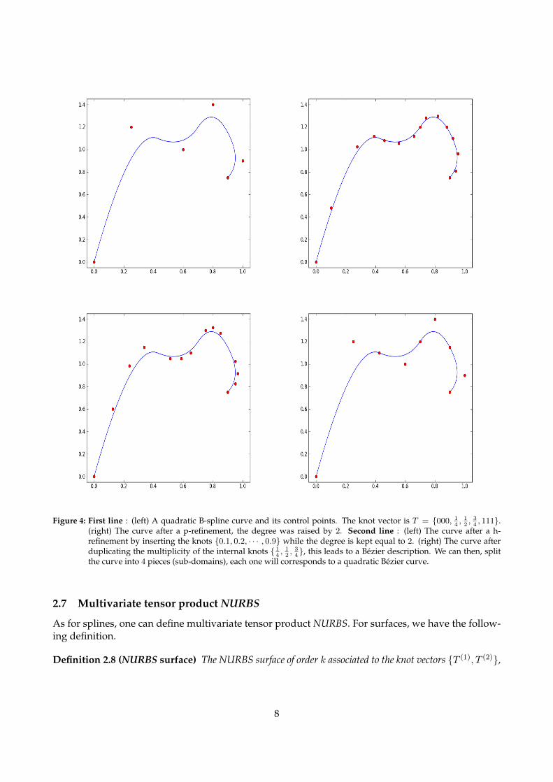
Figure 4: First line : (left) A quadratic B-spline curve and its control points. The knot vector is T = 000, 14, 12, 34, 111.

(right) The curve after a p-refinement, the degree was raised by 2. Second line : (left) The curve after a h-refinement by inserting the knots 0.1, 0.2, · · · , 0.9 while the degree is kept equal to 2. (right) The curve afterduplicating the multiplicity of the internal knots 1

4, 12, 34, this leads to a Bezier description. We can then, split

the curve into 4 pieces (sub-domains), each one will corresponds to a quadratic Bezier curve.

2.7 Multivariate tensor product NURBS

As for splines, one can define multivariate tensor product NURBS. For surfaces, we have the follow-ing definition.

Definition 2.8 (NURBS surface) The NURBS surface of order k associated to the knot vectors T (1), T (2),

8

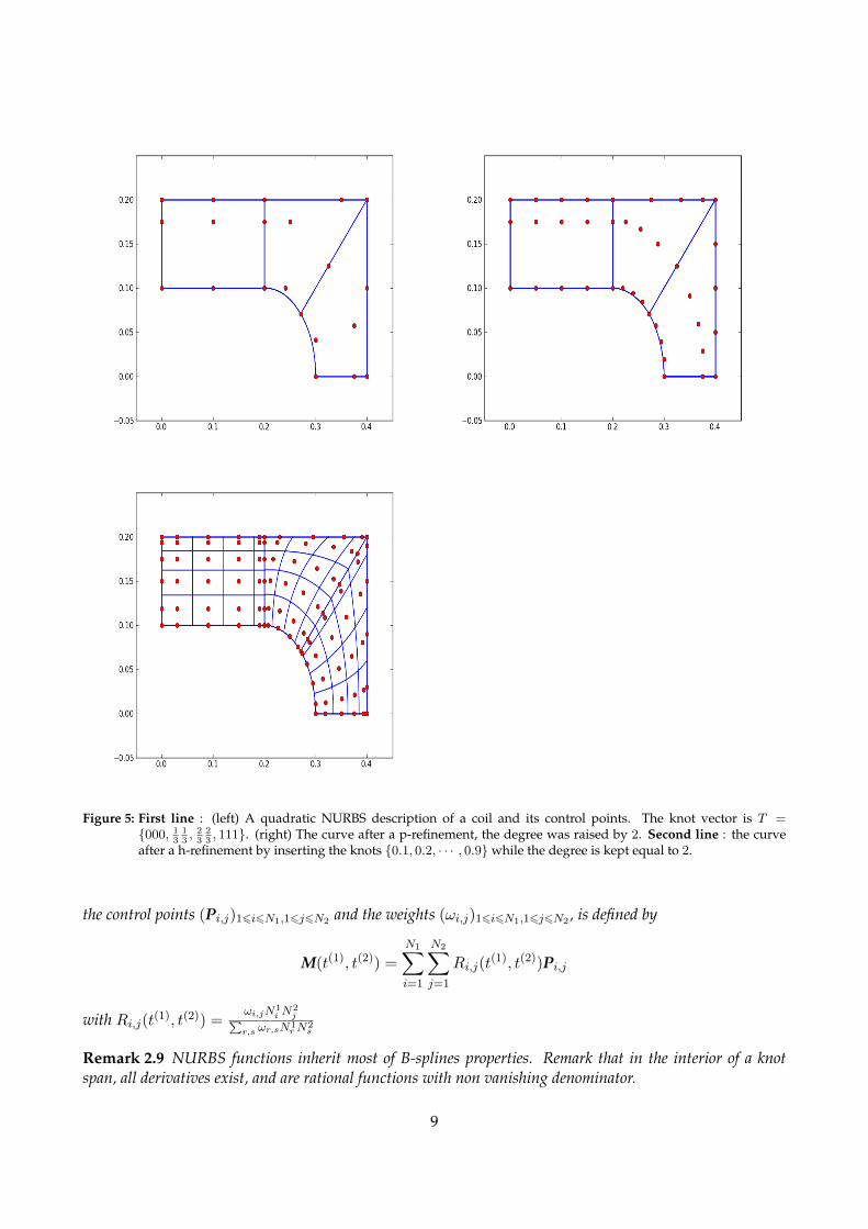
Figure 5: First line : (left) A quadratic NURBS description of a coil and its control points. The knot vector is T =000, 1

313, 23

23, 111. (right) The curve after a p-refinement, the degree was raised by 2. Second line : the curve

after a h-refinement by inserting the knots 0.1, 0.2, · · · , 0.9while the degree is kept equal to 2.

the control points (Pi,j)16i6N1,16j6N2 and the weights (ωi,j)16i6N1,16j6N2 , is defined by

M(t(1), t(2)) =

N1∑i=1

N2∑j=1

Ri,j(t(1), t(2))Pi,j

with Ri,j(t(1), t(2)) =ωi,jN

1i N

2j∑

r,s ωr,sN1rN

2s

Remark 2.9 NURBS functions inherit most of B-splines properties. Remark that in the interior of a knotspan, all derivatives exist, and are rational functions with non vanishing denominator.

9

nature of the curveω2 = 0 line0 < ω2 < 1 ellipse arcω2 = 1 parabolic arcω2 > 1 hyperbolic arc

Table 1: Modeling conics using NURBS.

We present here the definition of the perspective mapping. We construct the weighted control points Pωi =(ωixi, ωiyi, ωizi, ωi), then we define the B-spline curve in four-dimensional space as

Mω(t) =

N∑i=1

Nki (t)Pωi . (2.5)

For fundamental geometric operations on NURBS curves, we use the latest transformation and algorithms onB-spline curves.

Remark 2.10 NURBS functions allow us to model, exactly, much more domains than B-splines. In fact, allconics can be exactly represented with NURBS. For more details, see [34].

2.8 IsoGeometric Analysis

The idea behind the IGA method is to use the same functions that define the physical domain, toapproach the solution of a partial differential equation.In the sequel, we consider 2 knot vectors Tξ = ξ1, · · · , ξN1+p1+1 and Tη = η1, · · · , ηN2+p2+1. LetWξ = ωξ1, · · · , ω

ξN1 and Wη = ωη1 , · · · , ω

ηN2 be two weight sequences, and (Pij)16i6N1,16j6N2 a

sequence of control points. This defines a mapping

F(ξ, η) =∑

16i6N1,16j6N2

Rξi (ξ)Rηj (η)Pij (2.6)

that maps the rectangular patch [ξ1, ξN1 ] × [η1, ηN2 ] onto the physical domain Ω. Where Rξ and Rη

are NURBS functions defined by knot vectors Tξ and Tη, and weights Wξ and Wη.As said before, we consider only open knot vectors. Without loss of generality, we shall considerknot vectors of the form:

ξ1 = · · · = ξp1+1 = η1 = · · · = ηp2+1 = 0,

andξN1+1 = · · · = ξN1+p1+1 = ηN2+1 = · · · = ηN2+p2+1 = 1.

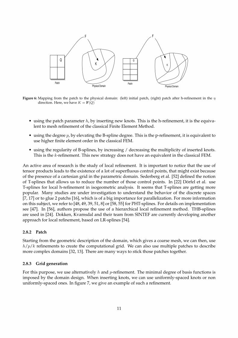
LetK be a cell in the physical domain. Q is the parametric associated cell and such thatK = F(Q).Let JF be the Jacobian of the transformation F, that maps any parametric domain point (ξ, η) into thephysical domain point (x, y) (figure 6).

2.8.1 Refinement strategies

Refining the grid can be done in 3 different ways. This is the most interesting aspects of B-splinesbasis,

10

Q

F

Patch Physical Domain

KQ

F

Patch Physical Domain

K

Figure 6: Mapping from the patch to the physical domain: (left) initial patch, (right) patch after h-refinement in the ηdirection. Here, we have K = F(Q)

• using the patch parameter h, by inserting new knots. This is the h-refinement, it is the equiva-lent to mesh refinement of the classical Finite Element Method.

• using the degree p, by elevating the B-spline degree. This is the p-refinement, it is equivalent touse higher finite element order in the classical FEM.

• using the regularity of B-splines, by increasing / decreasing the multiplicity of inserted knots.This is the k-refinement. This new strategy does not have an equivalent in the classical FEM.

An active area of research is the study of local refinement. It is important to notice that the use oftensor products leads to the existence of a lot of superfluous control points, that might exist becauseof the presence of a cartesian grid in the parametric domain. Sederberg et al. [52] defined the notionof T-splines that allows us to reduce the number of those control points. In [22] Dorfel et al. useT-splines for local h-refinement in isogeometric analysis. It seems that T-splines are getting morepopular. Many studies are under investigation to understand the behavior of the discrete spaces[7, 17] or to glue 2 patchs [16], which is of a big importance for parallelization. For more informationon this subject, we refer to [48, 49, 39, 51, 8] or [58, 55] for PHT-splines. For details on implementationsee [47]. In [56], authors propose the use of a hierarchical local refinement method. THB-splinesare used in [24]. Dokken, Kvamsdal and their team from SINTEF are currently developing anotherapproach for local refinement, based on LR-splines [54].

2.8.2 Patch

Starting from the geometric description of the domain, which gives a coarse mesh, we can then, useh/p/k refinements to create the computational grid. We can also use multiple patches to describemore complex domains [32, 13]. There are many ways to stick those patches together.

2.8.3 Grid generation

For this purpose, we use alternatively h and p-refinement. The minimal degree of basis functions isimposed by the domain design. When inserting knots, we can use uniformly-spaced knots or nonuniformly-spaced ones. In figure 7, we give an example of such a refinement.

11

Figure 7: Grid generation: (left) The coarsest mesh, (right) Domain after h-refinement. The minimal degree of basis func-tions is 2 in this example.

3 Introducing Πgasus

In this section, we will consider the resolution of an elliptic partial differential equation on a squaredomain Ω. We will see how we can recover the classical FEM language, for the IGA approach. Wealso will separate the different differential operators in the equation and how we can construct themusing Πgasus .

Let us consider the following problem:

For given functions A, f, b, find u such that:−∇ · (A∇u) + bu = f ,Ω

u = 0 , ∂Ω(3.7)

Introducing the matrix :Σ = (Σi,j)16i,j6n

and the vectors :L = (Li)

T16i6n−nD

[uh] = ([uh]i)T16i6n

where, we denote for i, j ∈ 1, .., n

Σi,j =

∫Ω∇ϕi A∇ϕj dΩ +

∫Ωb ϕi ϕj dΩ

Li =

∫Ωf ϕi dΩ

here, n denotes the dimension of the discrete space and nD the number of Dirichlet elements.

12

Using a variational formulation and the Green’s formulae, we know that after discretization, wehave to solve the linear system:

Σ [uh] = L .

The matrix Σ is nothing else but the sum of the Stiffness matrix S and Mass matrix M .

S =

∫Ω∇ϕi A∇ϕj dΩ

M =

∫Ωb ϕi ϕj dΩ

In practice, the user will need to define, discretize and assemble the two differential operatorsM andS. To do so, we must start by defining the discrete FE space (see subsection 3.1), with the appropriateboundary conditions and set the computational grid. Then, he needs to define two fields, one for theright hand side term, and the other for the solution of the pde (see subsection 3.2). Finally, he definesthe discretized differential operators M and S (see subsection 3.3). In the following subsections, wewill detail and explain each step of a typical Πgasus script. For instance, we will solve the Poisson’sequation on the unit square domain with the source term :

f(x, y) = 8π2 sin(2πx) sin(2πy)

and the analytical solutionu(x, y) = sin(2πx) sin(2πy)

3.1 Spaces Definition

The Galerkin Finite Element Method relies on the fact that we approach the inifinite dimensionalspaces, where the unknowns may live, by a sequence of finite dimensional subspaces. WithΠgasus we recover this approach and start by creating these finite dimensional subspaces.

1 # def ine the d i s c r e t e space2 V = space (as_file=ls_domain )3 # s e t boundary condi t ions4 # here we use Homogeneous D i r i c h l e t on whole the boundary5 V .dirichlet (faces= [ [ 1 , 2 , 3 , 4 ] ] )6 V .set_boundary_conditions ( )

The discrete space needs a geometry that may be given by in XML or HDF5 file. Once the space wasdefined, we have to associate a grid (quadrature points).

1 # c r e a t e a grid ( using Gauss−Legendre quadrature points )2 V .create_grids (type=” legendre ” , k=lpi_glorder )

3.2 Fields Definition

The Field object can be used to define either the right hand side term or the unknown.

1 # def ine the r i g h t hand s ide2 func_f = lambda x ,y : [ 2 . 0 * ( ( 2 *pi ) * * 2 ) * sin ( 2 *pi * x ) * sin ( 2 *pi * y ) ]3 F_V = field (space=V , func = func_f )45 # t h i s i s the unknown6 func_u = lambda x ,y : [sin ( 2 *pi * x ) * sin ( 2 *pi * y ) ]7 U_V = field (space=V , func = func_u )

13

3.3 Matrices Definition

Here, we show how we can construct and assembly the differential operators involved in our PDE.The Mass matrix operator is of the form Mass∫

Ωf([u],x) ϕb ϕb′ dΩ

while the Stiffness matrix is ∫Ω

(A([u],x) ∇ϕb) · ∇ϕb′ dΩ

In this example, we have f([u],x) = 1.0 and A([u],x) = IdR3 is the identity matrix in R3. UsingΠgasus , this can be defined as

1 # def ine the mass matrix2 func_mass = lambda x ,y : [ 1 . 0 ]3 M_V = matrix (spaces= [V , V ] , ai_type=MASS , func=func_mass )4 # def ine the s t i f f n e s s matrix5 func_stiff = lambda x ,y : [ 1 . 0 , 0 . 0 , 0 . 0 , 1 . 0 ]6 S_V = matrix (spaces= [V , V ] , ai_type=STIFFNESS , func=func_stiff )

3.4 Initialization

Once we have defined all the operators and fields that we need to model our PDE, we have to initial-ize Πgasus .

1 fe .initialize ( )

3.5 Assembling Process

Using the function assembly, we can assemble the operators that we need. We can imagine, that fora given problem, one of the operators will remain unchanged while the others may change at eachiteration. In this case, the user can specify which matrices or fields to assemble, by given it in thematrices or fields lists.

1 fe .assembly (matrices= [M_V , S_V ] , fields= [F_V ] )

3.6 Solving the linear system

You can either use the integrated linear solver for Πgasus , or export matrices to python and useyour favorite solver. Next, we show how the later one can be done using spsolve and SuperLU.

1 # export matr ices to scipy−c s r format2 Mass_V = M_V .to_csr ( )3 Stiffness_V = S_V .to_csr ( )4 Sigma = Mass_V + Stiffness_V56 # export the r i g h t hand s ide7 lpr_rhs = F_V .get ( )89 # solv ing using spsolve

14

10 from scipy .sparse .linalg import spsolve11 lpr_u = spsolve ( Sigma , lpr_rhs )1213 # solv ing using splu14 from scipy .sparse .linalg import splu15 op_Sigma = splu (Sigma .tocsc ( ) ) # F a c t o r i z a t i o n16 lpr_u = op_Sigma .solve ( lpr_rhs )1718 # import the r i g h t hand s ide i n t o Pigasus19 U_V .set (lpr_u )

Remark 3.1 The user can also manipulate the objects Fields and matrices using the operators *=, += or.dot(. . . )

In (figure 8), we plot the numerical solution of Poisson’s equation on the unit square.

Figure 8: Poisson’s equation on the unit square : plot of the numerical solution

3.7 Computing the error norm

In Πgasus , the norms are modeled as operators on fields. The user can compute the classical L2, H1,etc, . . . , norms for a given field.An example of declaration is:

1 N_U = norm ( field=U_V , type=NORM_L2 )

Here we show how to compute the L2 norm.

1 # s e t the NURBS/B−s p l i n e s c o e f f i c i e n t s ,2 # in the case of using e x t e r n a l s o l v e r3 U_V .set (lpr_u )4 # assemble the norm operator5 fe .assembly (norms= [N_U ] )67 lr_norm = N_U .get ( )

15

As seen, through the previous example, Πgasus is designed following the classical FEM lan-guage. In the next section, we shall give much more detail about the architecure of Πgasus and theoffered notions and objects.

4 Dive into Πgasus

In this section, we will introduce some advanced utilities and give much more precision on the designof the library. We start by introducing the Geometry module, the architecture and then present thefundamentals concepts/objects.

4.1 Geometry Module

An important difference between CAD and the numerical simulation worlds, is the nature of a givendomain. In CAD, a circle is a curve, but in order to solve the Poisson’s equation (for example) ona circular domain (for example) we need a 2D description. Hence, even if there are many powerfultools for CAD, they present at least this disadvantage. It is also complicated for mathematicians andphysicists to use such tools. Remember that the user wants a volume description of its domain. Formore details, we refer to [35, 36, 37, 12]. For all these reasons, we prefered to developp our ownmodule for geometry, with a simple interface for the user and a classical XML format. We havealso added HDF5 format to handle heavy data, as the user may want to store his domain after therefinement process.

4.1.1 Formats

There are two ways to store the geometry. For heavy data (especially in 3D), you have to use theHDF5 format. Weights are stored here as the d + 1 component of the control point (where d is thespace dimension). In (Appendix, source code 1) we show the XML-file of the linear description of theunit square.

4.1.2 Geometry utilities

In (Appendix, source code 2), we show how to use a p-refinement. Now let’s take the linear descriptionof the unit square, and perform

1. a p-refinement: we will elevate the spline degree : +1 in the ξ-direction and +1 in the η-direction,

2. an h-refinement: we will insert 0.25, 0.5, 0.75 in the ξ-direction and 0.3, 0.7 in the η-direction,.

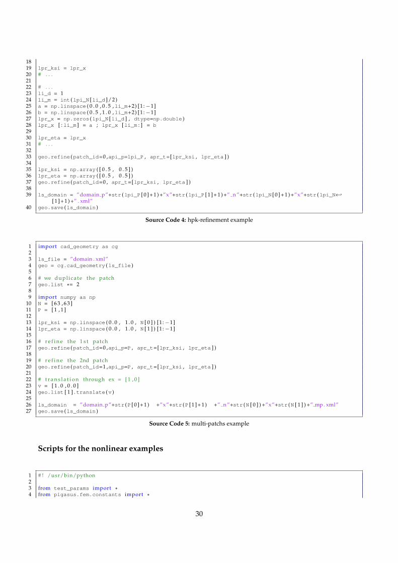
The detail of the script is given in (Appendix, source code 3). In order to do a k-refinement, you caneither do a h-refinement then a p-refinement, or do directly a hp-refinement with duplicated knots(Appendix, source code 4). In (Appendix, source code 5) we show a simple example of how we canduplicate a given geometry and modify it to have a multi-patchs description.

Remark 4.1 We have developed a 2D-CAD designer tool, in order to manipulate and generate directly, thevolume description of the computational domain [43].

16

4.2 Πgasus architecture

In the following subsection, we present the architecture behind Πgasus .Although there is no Singleton notion in Python, we can define an alternative using the followingclassical idea.

1 def singleton (cls ) :2 instances = 3 def getinstance ( ) :4 i f cls not in instances :5 instances [cls ] = cls ( )6 return instances [cls ]7 return getinstance

Then, we can define the common obj class, which will contain all spaces, fields, matrices, . . . , dec-larations. Each time the user will declare a new space (for example), it will be automatically addedinto the common obj.spaces list.

1 @singleton2 c l a s s common_obj (object ) :3 def __init__ ( s e l f ) :4 # . . .5 # importing the Fortran module6 # . . .7 import pyfem as py8 s e l f .pyfem = py .pyfem9 # . . .

1011 # . . .12 # def in ing o b j e c t s l i s t s13 # . . .14 s e l f .fields = [ ]15 s e l f .matrices = [ ]16 s e l f .spaces = [ ]17 s e l f .mappings = [ ]18 s e l f .grids = [ ]19 s e l f .norms = [ ]20 # . . .

Remark 4.2 All objects (Fields, Matrices and Norms) are stored with a sub-domain (patch) id. As seen before,the user will use the fundamental geometric operations, to split the computational domain into many sub-domains while keeping the geometry exact. Then he will provide this new description to construct the FiniteElement space.

4.2.1 Spaces

The notion of spaces has been introduced in the previous section. Let us just give some additionalremarks. The user can define a space using an exterior mapping (not defined by the IGA approach).For example, he can give an analytic mapping (or a new metric) or even a CAD-description usingsplines or nurbs.

Remark 4.3 We have choosed to use a tensorial approach for Πgasus . This means that inside each element,the grid is viewed as n-arrays rather than an array of Rn. A patch is a collection of elements. The user canstick patchs together by using the duplicate function.

17

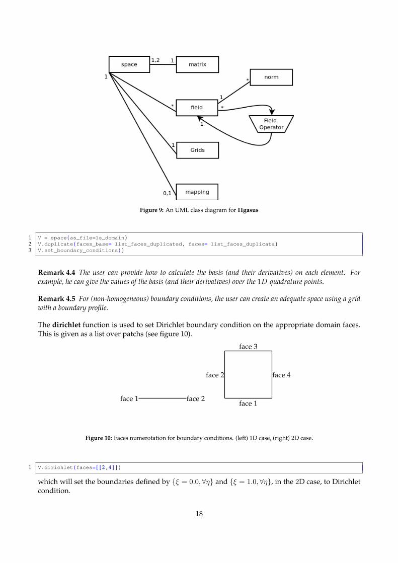
Figure 9: An UML class diagram for Πgasus

1 V = space (as_file=ls_domain )2 V .duplicate (faces_base= list_faces_duplicated , faces= list_faces_duplicata )3 V .set_boundary_conditions ( )

Remark 4.4 The user can provide how to calculate the basis (and their derivatives) on each element. Forexample, he can give the values of the basis (and their derivatives) over the 1D-quadrature points.

Remark 4.5 For (non-homogeneous) boundary conditions, the user can create an adequate space using a gridwith a boundary profile.

The dirichlet function is used to set Dirichlet boundary condition on the appropriate domain faces.This is given as a list over patchs (see figure 10).

face 1 face 2face 1

face 4

face 3

face 2

Figure 10: Faces numerotation for boundary conditions. (left) 1D case, (right) 2D case.

1 V .dirichlet (faces= [ [ 2 , 4 ] ] )

which will set the boundaries defined by ξ = 0.0, ∀η and ξ = 1.0, ∀η, in the 2D case, to Dirichletcondition.

18

In the case where we use a multi-patch description, the user can specify the Dirichlet boundarycondition as shown in figure 11.

1 V .dirichlet (faces= [ [ 1 , 2 , 3 ] , [ 1 , 3 , 4 ] ] )

1 1

2

3 3

44 2Ω1 Ω2

Figure 11: Faces numerotation for boundary conditions for a multi-patchs domain in the 2D case.

The duplicate function can be used to set periodic boundary conditions or to stick patchs togetherwith a C0 condition. It tells Πgasus that all basis defined by ”face-base” have the same ID (see [31]for details on FEM connectivities structures) as those by ”face”. Both ”face-base” and ”face” must belists of couples [patch id, num face]. To set a periodic boundary condition:

1 V .duplicate (faces_base= [ [ 0 , 1 ] ] , faces= [ [ 0 , 3 ] ] )

To stick two patchs together:

1 V .duplicate (faces_base= [ [ 0 , 4 ] ] , faces= [ [ 1 , 2 ] ] )

4.2.2 Vectorial spaces

The basic definition of spaces, leads to scalar functions. In order to define a vectorial space, the usermust proceed as on paper, he starts by defining spaces for each coordinate, on the patch and withouta mapping, then he defines the whole space as a vect space. In the following example, we show atypical construction, for the Maxwell’s time domain problem [45].

In 2D domains, Maxwell’s equations can be decoupled into two systems. The first involvingthe (Ex, Ey, Hz) components is called the Transverse Electric (TE) mode, and the second, involvingthe (Hx, Hy, Ez) components is called the Transverse Magnetic (TM) mode. As both modes can bediscretized in the same manner, The TE mode reads

∂E

∂t− rotH = −J, (4.8)

∂H

∂t+ rot E = 0, (4.9)

div E = ρ, (4.10)

where the components are defined by E =

(ExEy

), H = Hz . Let us define the following scalar spaces

:V = Sp,pα,α, W1 = Sp,p−1

α,α−1, W2 = Sp−1,pα−1,α

and the vectorial spaceW = W1×W2

19

The discrete spaces V and W are involved in the DeRham sequence [45].

1 p = 32 n = 6334 ls_etiq = ” p ”+str (p ) +”x”+str (p ) +” n ”+str (n ) +”x”+str (n )56 ls_domain_V = ”domain p”+str (p ) +”x”+str (p ) +” n ”+str (n ) +”x”+str (n ) +” . xml”7 ls_domain_W1 = ”domain p”+str (p ) +”x”+str (p - 1 ) +” n ”+str (n ) +”x”+str (n ) +” . xml”8 ls_domain_W2 = ”domain p”+str (p - 1 ) +”x”+str (p ) +” n ”+str (n ) +”x”+str (n ) +” . xml”9 ls_domain_W = ”domain W . xml”

1011 # * * * * * * * * * * * * * * * * * * * * * * * * * * * * * * * * * * * * * * *12 # D e f i n i t i o n of the space V13 # * * * * * * * * * * * * * * * * * * * * * * * * * * * * * * * * * * * * * * *14 V = space (as_file=ls_domain_V )15 V .set_boundary_conditions ( )16 V .create_grids (type=” legendre ” , k=lpi_ordregl )17 # * * * * * * * * * * * * * * * * * * * * * * * * * * * * * * * * * * * * * * *1819 # * * * * * * * * * * * * * * * * * * * * * * * * * * * * * * * * * * * * * * *20 # D e f i n i t i o n of the space W121 # * * * * * * * * * * * * * * * * * * * * * * * * * * * * * * * * * * * * * * *22 W1 = space (as_file=ls_domain_W1 )23 W1 .set_boundary_conditions ( )24 W1 .create_grids (space=V )25 # * * * * * * * * * * * * * * * * * * * * * * * * * * * * * * * * * * * * * * *2627 # * * * * * * * * * * * * * * * * * * * * * * * * * * * * * * * * * * * * * * *28 # D e f i n i t i o n of the space W229 # * * * * * * * * * * * * * * * * * * * * * * * * * * * * * * * * * * * * * * *30 W2 = space (as_file=ls_domain_W2 )31 W2 .set_boundary_conditions ( )32 W2 .create_grids (space=V )33 # * * * * * * * * * * * * * * * * * * * * * * * * * * * * * * * * * * * * * * *3435 # * * * * * * * * * * * * * * * * * * * * * * * * * * * * * * * * * * * * * * *36 # D e f i n i t i o n of the space W as W1 x W237 # * * * * * * * * * * * * * * * * * * * * * * * * * * * * * * * * * * * * * * *38 W = space_vect (spaces= [W1 ,W2 ] )39 W .set_boundary_conditions ( )40 W .create_grids (space=V )41 # * * * * * * * * * * * * * * * * * * * * * * * * * * * * * * * * * * * * * * *

4.2.3 Fields

As said previously, the notion of Field is intended to model a right hand side or an unknown. Nextwe list some of its attributs:

• space : This is the discrete space on which the field is defined.

• func : This is a given function for the field. It can be used either for the source term or the exactsolution.

• type : This is the projection/interpolation type.

• operator : This is used to apply an operator to a field, defined previously.

• field : This is the operande for the operator (must be given if the type is FIELD OPERATOR).

• func arguments : This is a list of fields used for a non-linear field (i.e. f([g],x)).

20

Remark 4.6 The user can define a field as a function of a list of fields. In the following example, we show howto model a term of the form :

f(u, x, y) = u2 + x2∂xu+ (x+ y)∂yu

In fact, we will need to define a new field u2 = v · ∇u which is a FIELD OPERATOR of type GRAD appliedon the fields u with an argument function v = [x2, x+ y].

1 # . . .2 # Defining the F i e l d Operator3 # . . .4 func_v = lambda x ,y : [x ˆ 2 , x+y ]5 U2 = field (space=V , operator=GRAD , field=U , func = func_v )6 # . . .78 # . . .9 # t h i s i s the non−l i n e a r part

10 # . . .11 func_F = lambda list_F ,x ,y : [list_F [ 0 ] ˆ 2 + list_F [ 1 ] ]12 F = field (space=V , func = func_F , func_arguments= [U ,U2 ] )13 # . . .

4.2.4 Matrices

A matrix ise stored naturally in a compact format thanks to its profile. The latter is easily computedthanks to the spaces connectivities. In order to construct a matrix, you need to specify the followingparameters:

• space : This is a couple of the discrete spaces on which the Differential Operator is defined.

• ai type : This is the type of the Differential Operator (MASS, STIFFNESS, ADVECTION, ...)

• func : This is a given parameter function for the matrix.

• matrices : This is used to construct a composed (block) matrix.

• transpose : If we want to transpose the matrix during the construction.

• func arguments : This is a list of fields used for a non-linear field (i.e. f([u],x)).

• addto : if we want to add the local element matrix directly to a global matrix previously defined.This will reduce the memory cost.

In table 2, we give the list of the implemented Differential Operators.

Operator ContributionMass

∫Ω f([u],x) ϕb ϕb′ dΩ

Stiffness∫

Ω(A([u],x)∇ϕb) · ∇ϕb′ dΩAdvection

∫Ω v([u],x) · ∇ϕb ϕb′ dΩ

Second derivatives∫

Ω v([u],x) · D2ϕb dΩ

Table 2: List of the implemented Differential operators

21

The user can also create Block-matrices or import a matrix. In the following example we showhow to construct a Block-Matrix. The user can choose which part to update during the assemblingprocess.

1 M_V = matrix (matrices= [ [A_1 ,B_1 ] , [C_1 ,D_1 ] ] )

and then, he can change the blocks by calling

1 M_V .set (matrices= [ [A_2 ,B_2 ] , [C_2 ,D_2 ] ] )

Where each two matrices X1 and X2 (X ∈ A,B,C,D) are defined on the same spaces, and havethe same profile. The user can choose which matrices to update, by calling

1 # M i s a Block−matrix = [ [A, B ] , [ C,D] ] defined previously by2 # M = matrix ( matr ices = [ [A, B ] , [ C,D] ] )3 # i f f o r example , only A and D must be re−evaluated then the user must c a l l45 M .assembly ( [ [ True , Fa l se ] , [ False , True ] ] )

4.2.5 Grids

Πgasus offers different types of grids. The user can associate to the discrete space, a volume, a surface,an edge or a boundary grid. The volume, surface, edge profiles are related to the elements, while theboundary profile is for the whole patch (sub-domain). Here is an example of how to create a grid fora given discrete space.

1 # * * * * * * * * * * * * * * * * * * * * * * * * * * * * * * * * * * * * * * *2 # D e f i n i t i o n of the space V3 # * * * * * * * * * * * * * * * * * * * * * * * * * * * * * * * * * * * * * * *4 V = space (as_file=ls_domain_V )5 V .set_boundary_conditions ( )6 V .create_grids (type=” legendre ” , k=lpi_ordregl , profile=”boundary” )7 # * * * * * * * * * * * * * * * * * * * * * * * * * * * * * * * * * * * * * * *

By grids, we mean, by default, quadrature ones. The user can use the predefined ones, or gives hisown grids, as follows:

1 # * * * * * * * * * * * * * * * * * * * * * * * * * * * * * * * * * * * * * * *2 # D e f i n i t i o n of the space V3 # * * * * * * * * * * * * * * * * * * * * * * * * * * * * * * * * * * * * * * *4 V = space (as_file=ls_domain_V )5 V .set_boundary_conditions ( )6 V .create_grids (list_nodes=list_x , list_weights=list_w )7 # * * * * * * * * * * * * * * * * * * * * * * * * * * * * * * * * * * * * * * *

The user can also create a grid without associating it to any space. This may be interesting if he wantsto take advantage of the B-splines and NURBS tranformations, in order to developp, for example, aFinite Difference code.

1 # * * * * * * * * * * * * * * * * * * * * * * * * * * * * * * * * * * * * * * *2 # D e f i n i t i o n of the grid G3 # * * * * * * * * * * * * * * * * * * * * * * * * * * * * * * * * * * * * * * *4 geo = cg .cad_geometry (ls_domain )5 G = grids (profile=”volume” , api_k=lpi_ordregl , ao_geometry=geo .list [ : ] , as_type=” legendre ” )

22

6 # * * * * * * * * * * * * * * * * * * * * * * * * * * * * * * * * * * * * * * *

In addition, Πgasus offers the possibility to create, manipulate a metric object and associate it to agrid. Remember that when using a CAD-description to manipulate the metric, we never need tostore the whole grid. On each element, we only store the 1D array, the grid will be constructed, onthe fly, at each assembling step.

1 # * * * * * * * * * * * * * * * * * * * * * * * * * * * * * * * * * * * * * * *2 # D e f i n i t i o n of Metr ics3 # * * * * * * * * * * * * * * * * * * * * * * * * * * * * * * * * * * * * * * *45 # . . .6 # using a CAD−d e s c r i p t i o n7 # . . .8 M1 = metric (geometry=geo .list [ : ] )9 # . . .

1011 # . . .12 # using an a n a l y t i c a l funct ion13 # . . .14 F = lambda r ,t : [r * np .cos ( 2 . * np .pi * t ) , r * np .sin ( 2 . * np .pi * t ) ]1516 DF = lambda r , t : [np .cos ( 2 . * np .pi * t ) \17 , - 2 . * np .pi * r * np .sin ( 2 . * np .pi * t ) \18 , np .sin ( 2 . * np .pi * t ) \19 , 2 . * np .pi * r * np .cos ( 2 . * np .pi * t ) ]2021 M2 = metric (analytic= [F ,DF ] )22 # . . .2324 # . . .25 # using a l i s t of points and d e r i v a t i v e s26 # . . .27 M3 = metric (points=lpr_points )28 # . . .2930 # * * * * * * * * * * * * * * * * * * * * * * * * * * * * * * * * * * * * * * *

Then we can associate the metric to a grid, as the following.

1 # * * * * * * * * * * * * * * * * * * * * * * * * * * * * * * * * * * * * * * *2 # D e f i n i t i o n of the grid G3 # * * * * * * * * * * * * * * * * * * * * * * * * * * * * * * * * * * * * * * *4 geo = cg .cad_geometry (ls_domain )5 G = grids (type=” legendre ” , k=lpi_ordregl , metric=Met )6 # * * * * * * * * * * * * * * * * * * * * * * * * * * * * * * * * * * * * * * *

4.2.6 Diagnostics

The user can apply different operators to a given field. Once for example, you have the Finite Elementdescription, you can ask Πgasus to evaluate the field or its derivatives. Now let’s take the exampleof Anisotropic Diffusion, which writes :

∂tu−∇ · (K∇u) = f, Ω (4.11)u = 0, ∂Ω (4.12)

23

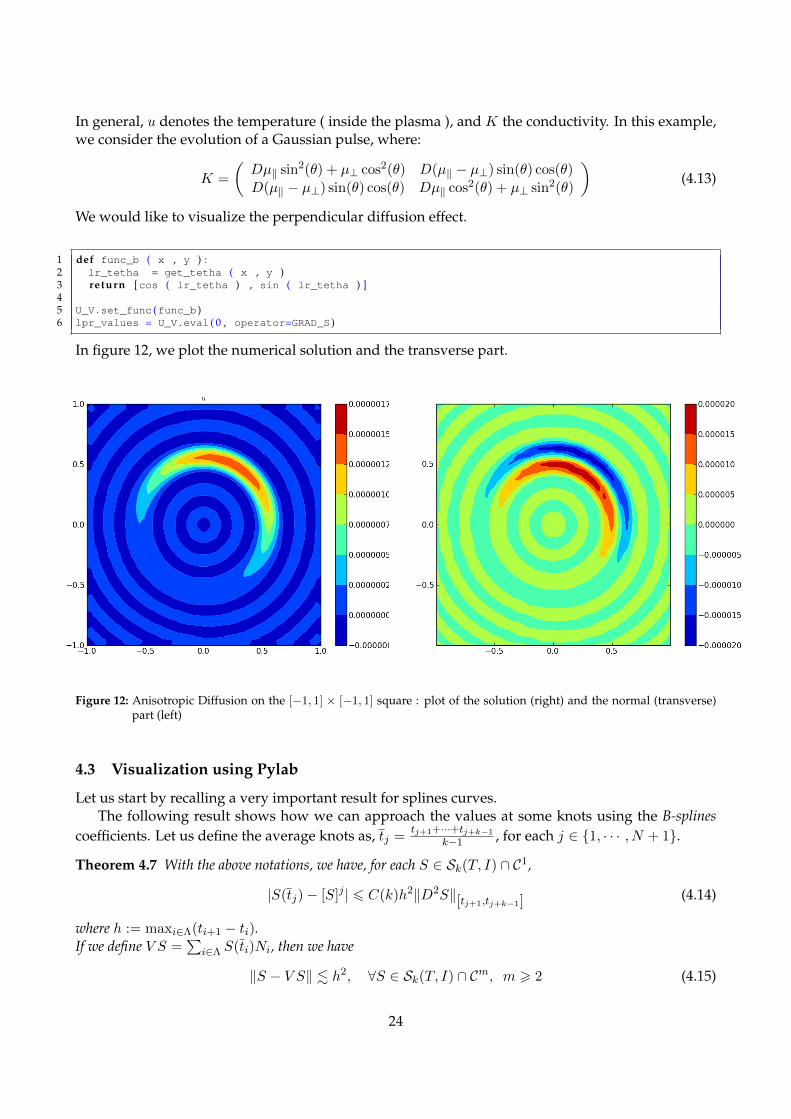
In general, u denotes the temperature ( inside the plasma ), and K the conductivity. In this example,we consider the evolution of a Gaussian pulse, where:

K =

(Dµ‖ sin2(θ) + µ⊥ cos2(θ) D(µ‖ − µ⊥) sin(θ) cos(θ)

D(µ‖ − µ⊥) sin(θ) cos(θ) Dµ‖ cos2(θ) + µ⊥ sin2(θ)

)(4.13)

We would like to visualize the perpendicular diffusion effect.

1 def func_b ( x , y ) :2 lr_tetha = get_tetha ( x , y )3 return [cos ( lr_tetha ) , sin ( lr_tetha ) ]45 U_V .set_func (func_b )6 lpr_values = U_V .eval ( 0 , operator=GRAD_S )

In figure 12, we plot the numerical solution and the transverse part.

Figure 12: Anisotropic Diffusion on the [−1, 1] × [−1, 1] square : plot of the solution (right) and the normal (transverse)part (left)

4.3 Visualization using Pylab

Let us start by recalling a very important result for splines curves.The following result shows how we can approach the values at some knots using the B-splines

coefficients. Let us define the average knots as, tj =tj+1+···+tj+k−1

k−1 , for each j ∈ 1, · · · , N + 1.

Theorem 4.7 With the above notations, we have, for each S ∈ Sk(T, I) ∩ C1,

|S(tj)− [S]j | 6 C(k)h2‖D2S‖[tj+1,tj+k−1] (4.14)

where h := maxi∈Λ(ti+1 − ti).If we define V S =

∑i∈Λ S(ti)Ni, then we have

‖S − V S‖ . h2, ∀S ∈ Sk(T, I) ∩ Cm, m > 2 (4.15)

24

As we can notice, the results of this form are important; we do not need to evalute the spline surfacefor visualization. We will only need to associate at each average knot, the correspondant coefficient.In the next example, we show how to do a fast-plot of a given field:

1 # Default c a l l2 F_V .fast_plot ( )

The function fast plot has the following arguments:

ai patch id the current patch,

useControlPoints is True if the B-slines coefficients will be associated to the control points as a firstapproximation,

savedPoints used if useControlPoints is False. If it is True, the user must provide list P.

list P a list of the associated points to B-slines coefficients.

The user still has the possibility to create his own grid and then evaluate the field.

4.4 Parallelization

Πgasus was designed in order to be parallelized, even if the current version is sequential. In thefuture it will be possible to use generic frameworks as Murge [27], PetSc [5], Hips [23] and have adirect link with some linear solvers (Pastix [27], Mumps [2, 3]).

5 Application to a non-linear equation

In this section, we show as an application of IGA, the resolution of a non-linear partial differentialequation. We will present two methods: Picard and Newton’s algorithms.In the sequel, we shall consider the following problem:Find u such that:

−∇ · (A∇u) +Bu = F (x, u) ,Ωu = 0 , ∂Ω

(5.16)

Let Vh be the discrete space, such that Vh = spanϕb, b ∈ 1, · · · , n, then the variational formula-tion of (5.16) is : ∫

Ω(A∇u) · ∇ϕb +

∫ΩBuϕb =

∫ΩF (x, u)ϕb, ∀b ∈ 1, · · · , n (5.17)

thus, by expanding uh over Vh, using uh =∑

b∈1,··· ,n[u]bϕb, we get :∑b∈1,··· ,n

[u]b∫

Ω(A∇ϕb) · ∇ϕb′ +

∫ΩBϕbϕb′ =

∫ΩF (x, uh)ϕb′ , ∀b′ ∈ 1, · · · , n (5.18)

this leads to solve the problem :

S[u] = F([u]) (5.19)

where,

Sb,b′ =

∫Ω

(A∇ϕb) · ∇ϕb′ +∫

ΩBϕbϕb′ , ∀b, b′ ∈ 1, · · · , n (5.20)

F([u])b′ =

∫ΩF (x, uh)ϕb′ , ∀b′ ∈ 1, · · · , n (5.21)

25

5.1 Picard’s algorithm

To solve iteratively 5.19, let us start with the Picard algorithm, which is the simplest one but also theless accurate.

1. X0 is given,

2. knowing Xn, we solve :

SXn+1 = F(Xn) (5.22)

5.2 Newton’s algorithm

Let us define the function :

g(X) = SX −F(X) (5.23)

thus [u] is a zero of the function g. To solve 5.19, we use Newton’s method. As Jg(X) = S −JF(X), theNewton’s method is:

• X0 is given,

• knowing Xn, we solve :

Jg(Xn)(Xn+1 −Xn) = −g(Xn) (5.24)

The algorithm is the following:

1. we compute the mass matrix associated to the function : ∂uF , i.e :

Mnb,b′ =

∫Ω∂uF (x,

∑b∈1,··· ,n

Xnb ϕb)ϕbϕb′ (5.25)

2. compute the term F(Xn):

[F(Xn)]b′ =

∫ΩF (x,

∑b∈1,··· ,n

Xnb ϕb)ϕb′ (5.26)

3. compute g(Xn):

g(Xn) = SXn −F(Xn) (5.27)

4. compute Jg(Xn):

Jg(Xn) = S − JF(Xn) = S −Mn (5.28)

5. solve Jg(Xn)(Xn+1 −Xn) = −g(Xn), and then find Xn+1

26

5.3 Numerical results : Example from combustion theory

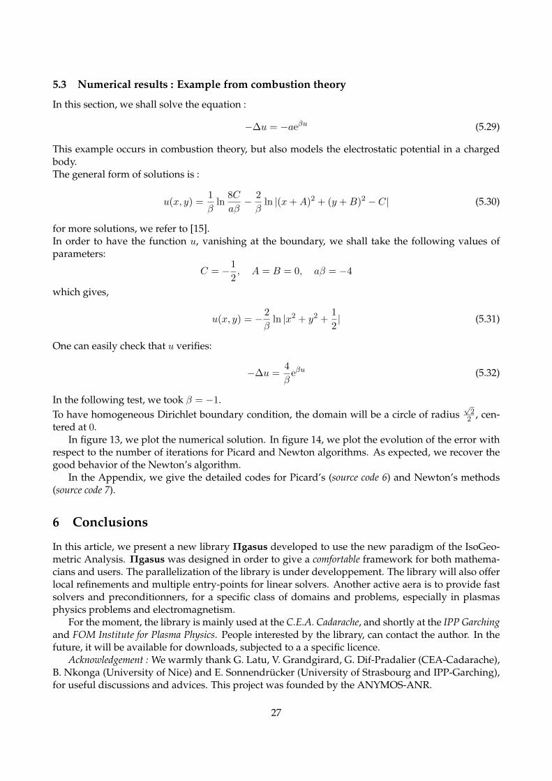
In this section, we shall solve the equation :

−∆u = −aeβu (5.29)

This example occurs in combustion theory, but also models the electrostatic potential in a chargedbody.The general form of solutions is :

u(x, y) =1

βln

8C

aβ− 2

βln |(x+A)2 + (y +B)2 − C| (5.30)

for more solutions, we refer to [15].In order to have the function u, vanishing at the boundary, we shall take the following values ofparameters:

C = −1

2, A = B = 0, aβ = −4

which gives,

u(x, y) = − 2

βln |x2 + y2 +

1

2| (5.31)

One can easily check that u verifies:

−∆u =4

βeβu (5.32)

In the following test, we took β = −1.To have homogeneous Dirichlet boundary condition, the domain will be a circle of radius

√2

2 , cen-tered at 0.

In figure 13, we plot the numerical solution. In figure 14, we plot the evolution of the error withrespect to the number of iterations for Picard and Newton algorithms. As expected, we recover thegood behavior of the Newton’s algorithm.

In the Appendix, we give the detailed codes for Picard’s (source code 6) and Newton’s methods(source code 7).

6 Conclusions

In this article, we present a new library Πgasus developed to use the new paradigm of the IsoGeo-metric Analysis. Πgasus was designed in order to give a comfortable framework for both mathema-cians and users. The parallelization of the library is under developpement. The library will also offerlocal refinements and multiple entry-points for linear solvers. Another active aera is to provide fastsolvers and preconditionners, for a specific class of domains and problems, especially in plasmasphysics problems and electromagnetism.

For the moment, the library is mainly used at the C.E.A. Cadarache, and shortly at the IPP Garchingand FOM Institute for Plasma Physics. People interested by the library, can contact the author. In thefuture, it will be available for downloads, subjected to a a specific licence.

Acknowledgement : We warmly thank G. Latu, V. Grandgirard, G. Dif-Pradalier (CEA-Cadarache),B. Nkonga (University of Nice) and E. Sonnendrucker (University of Strasbourg and IPP-Garching),for useful discussions and advices. This project was founded by the ANYMOS-ANR.

27

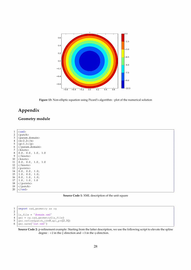
Figure 13: Non-elliptic equation using Picard’s algorithm : plot of the numerical solution

Appendix

Geometry module

1 <xml>2 <patch>3 <param domain>4 <n>2 ,2</n>5 <p>1 ,1</p>6 </param domain>7 <knots>8 0 . 0 , 0 . 0 , 1 . 0 , 1 . 09 </knots>

10 <knots>11 0 . 0 , 0 . 0 , 1 . 0 , 1 . 012 </knots>13 <points>14 0 . 0 , 0 . 0 , 1 . 0 ;15 1 . 0 , 0 . 0 , 1 . 0 ;16 0 . 0 , 1 . 0 , 1 . 0 ;17 1 . 0 , 1 . 0 , 1 . 018 </points>19 </patch>20 </xml>

Source Code 1: XML description of the unit square

1 import cad_geometry as cg23 ls_file = ”domain . xml”4 geo = cg .cad_geometry (ls_file )5 geo .refine (patch_id=0 ,api_p= [ 2 , 3 ] )6 geo .save ( ” out . xml” )

Source Code 2: p-refinement example: Starting from the latter description, we use the following script to elevate the splinedegree : +2 in the ξ-direction and +3 in the η-direction.

28

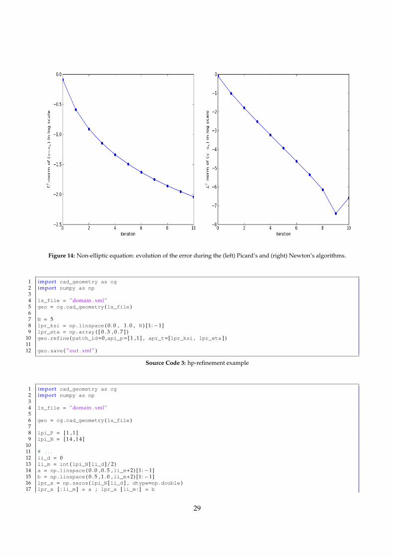
Figure 14: Non-elliptic equation: evolution of the error during the (left) Picard’s and (right) Newton’s algorithms.

1 import cad_geometry as cg2 import numpy as np34 ls_file = ”domain . xml”5 geo = cg .cad_geometry (ls_file )67 N = 58 lpr_ksi = np .linspace ( 0 . 0 , 1 . 0 , N ) [1 :−1]9 lpr_eta = np .array ( [ 0 . 3 , 0 . 7 ] )

10 geo .refine (patch_id=0 ,api_p= [ 1 , 1 ] , apr_t=[lpr_ksi , lpr_eta ] )1112 geo .save ( ” out . xml” )

Source Code 3: hp-refinement example

1 import cad_geometry as cg2 import numpy as np34 ls_file = ”domain . xml”56 geo = cg .cad_geometry (ls_file )78 lpi_P = [ 1 , 1 ]9 lpi_N = [ 1 4 , 1 4 ]

1011 # . . .12 li_d = 013 li_m = int (lpi_N [li_d ] /2 )14 a = np .linspace ( 0 . 0 , 0 . 5 ,li_m+2) [1 :−1]15 b = np .linspace ( 0 . 5 , 1 . 0 ,li_m+2) [1 :−1]16 lpr_x = np .zeros (lpi_N [li_d ] , dtype=np .double )17 lpr_x [ : li_m ] = a ; lpr_x [li_m : ] = b

29

1819 lpr_ksi = lpr_x20 # . . .2122 # . . .23 li_d = 124 li_m = int (lpi_N [li_d ] /2 )25 a = np .linspace ( 0 . 0 , 0 . 5 ,li_m+2) [1 :−1]26 b = np .linspace ( 0 . 5 , 1 . 0 ,li_m+2) [1 :−1]27 lpr_x = np .zeros (lpi_N [li_d ] , dtype=np .double )28 lpr_x [ : li_m ] = a ; lpr_x [li_m : ] = b2930 lpr_eta = lpr_x31 # . . .3233 geo .refine (patch_id=0 ,api_p=lpi_P , apr_t=[lpr_ksi , lpr_eta ] )3435 lpr_ksi = np .array ( [ 0 . 5 , 0 . 5 ] )36 lpr_eta = np .array ( [ 0 . 5 , 0 . 5 ] )37 geo .refine (patch_id=0 , apr_t=[lpr_ksi , lpr_eta ] )3839 ls_domain = ”domain p”+str (lpi_P [ 0 ] + 1 ) +”x”+str (lpi_P [ 1 ] + 1 ) +” n ”+str (lpi_N [ 0 ] + 1 ) +”x”+str (lpi_N←

[ 1 ] + 1 ) +” . xml”40 geo .save (ls_domain )

Source Code 4: hpk-refinement example

1 import cad_geometry as cg23 ls_file = ”domain . xml”4 geo = cg .cad_geometry (ls_file )56 # we d up l i c a t e the patch7 geo .list *= 289 import numpy as np

10 N = [ 6 3 , 6 3 ]11 P = [ 1 , 1 ]1213 lpr_ksi = np .linspace ( 0 . 0 , 1 . 0 , N [ 0 ] ) [1 :−1]14 lpr_eta = np .linspace ( 0 . 0 , 1 . 0 , N [ 1 ] ) [1 :−1]1516 # r e f i n e the 1 s t patch17 geo .refine (patch_id=0 ,api_p=P , apr_t=[lpr_ksi , lpr_eta ] )1819 # r e f i n e the 2nd patch20 geo .refine (patch_id=1 ,api_p=P , apr_t=[lpr_ksi , lpr_eta ] )2122 # t r a n s l a t i o n through ex = [ 1 , 0 ]23 v = [ 1 . 0 , 0 . 0 ]24 geo .list [ 1 ] . translate (v )2526 ls_domain = ”domain p”+str (P [ 0 ] + 1 ) +”x”+str (P [ 1 ] + 1 ) +” n ”+str (N [ 0 ] ) +”x”+str (N [ 1 ] ) +” mp . xml”27 geo .save (ls_domain )

Source Code 5: multi-patchs example

Scripts for the nonlinear examples

1 # ! /usr/bin/python23 from test_params import *4 from pigasus .fem .constants import *

30

5 from pigasus .fem .field import *6 from pigasus .fem .norm import *7 from pigasus .fem .grids import *8 from pigasus .fem .matrix import *9 from pigasus .fem .space import *

1011 import pigasus .fem .fem as fem12 fe = fem .fem (stdoutput=True ,ai_detail=0)1314 # * * * * * * * * * * * * * * * * * * * * * * * * * * * * * * * * * * * * * * *15 # D e f i n i t i o n of the space V16 # * * * * * * * * * * * * * * * * * * * * * * * * * * * * * * * * * * * * * * *17 V = space (as_file=ls_domain )18 V .dirichlet (faces= [ [ 1 , 2 , 3 , 4 ] ] )19 V .set_boundary_conditions ( )20 V .create_grids (type=” legendre ” , k=lpi_ordregl )21 # * * * * * * * * * * * * * * * * * * * * * * * * * * * * * * * * * * * * * * *2223 # * * * * * * * * * * * * * * * * * * * * * * * * * * * * * * * * * * * * * * *24 # D e f i n i t i o n of f i e l d s25 # * * * * * * * * * * * * * * * * * * * * * * * * * * * * * * * * * * * * * * *26 from numpy import log , exp2728 func_u0 = lambda x ,y : [− 2 . 0 * log ( x * * 2 + y * * 2 + 0 . 5 ) ]29 U0_V = field (space=V , func = func_u0 )3031 func_u = lambda x ,y : [− 2 . 0 * log ( x * * 2 + y * * 2 + 0 . 5 ) ]32 U_V = field (space=V , func = func_u )3334 # . . . t h i s i s the non−l i n e a r part35 def func_F (list_F , x , y ) :36 re turn [ 4 . 0 * exp ( list_F [ 0 ] ) ]37 F_V = field (space=V , func = func_F , func_arguments=[U_V ] )38 # * * * * * * * * * * * * * * * * * * * * * * * * * * * * * * * * * * * * * * *3940 # * * * * * * * * * * * * * * * * * * * * * * * * * * * * * * * * * * * * * * *41 # D e f i n i t i o n of norms42 # * * * * * * * * * * * * * * * * * * * * * * * * * * * * * * * * * * * * * * *43 N_U = norm (field=U_V , type=NORM_L2 )4445 # * * * * * * * * * * * * * * * * * * * * * * * * * * * * * * * * * * * * * * *46 # D e f i n i t i o n of matr ices47 # * * * * * * * * * * * * * * * * * * * * * * * * * * * * * * * * * * * * * * *48 func_mass = lambda x ,y : [ 1 . 0 ]49 M_V = matrix (spaces=[V , V ] , ai_type=MASS , func=func_mass )50 func_stiff = lambda x ,y : [ 1 . 0 , 0 . 0 , 0 . 0 , 1 . 0 ]51 S_V = matrix (spaces=[V , V ] , ai_type=STIFFNESS , func=func_stiff )52 # * * * * * * * * * * * * * * * * * * * * * * * * * * * * * * * * * * * * * * *5354 fe .initialize ( )5556 fe .assembly (matrices=[M_V , S_V ] , fields=[U0_V , U_V , F_V ] )5758 Mass_V = M_V .to_csr ( )59 Stiffness_V = S_V .to_csr ( )6061 from scipy .sparse .linalg import spsolve6263 # i n i t i a l i z a t i o n64 # lpr u = spsolve ( Mass V , U0 V . get ( ) )65 lpr_u = np .zeros (U_V .size )66 U_V .set (lpr_u ) ; np .savetxt ( ” runs/u 0 . t x t ” , lpr_u )6768 list_norm = [ ]6970 fe .assembly (norms=[N_U ] )71 list_norm .append (N_U .get ( ) )7273 # * * * * * * * * * * * * * * * * * * * * * * * * * * * * * * * * * * * * * * *

31

74 i = 075 miniter = i76 minerror = error77 list_minerror = [ ]78 lpr_u_old = lpr_u79 # * * * * * * * * * * * * * * * * * * * * * * * * * * * * * * * * * * * * * * *80 while ( ( error > tol ) and ( i < niter ) ) :8182 p r i n t ( ” i t e r a t i o n = ”+str (i ) )8384 i = i + 18586 F_V .reset ( )8788 fe .assembly (fields=[F_V ] )89 lpr_source = F_V .get ( )90 # p r i n t ”F ( u ) = ” , l p r s o u r c e91 lpr_u = spsolve ( Stiffness_V , lpr_source )9293 #computing the e r r o r between X ˆ ( n+1) and Xˆ n : X ˆ ( n+1) − Xˆ n94 lpr_delta = lpr_u − lpr_u_old95 lpr_u_old = lpr_u96 U_V .set (lpr_u )9798 error = max (abs (lpr_delta ) )99 i f ( minerror > error ) :

100 minerror = error101 miniter = i102 list_minerror .append (minerror )103104 i f ( np .mod ( i , nfreq ) == 0 ) :105 numdiag = i / nfreq106107 np .savetxt ( ” runs/u ”+str (numdiag ) +” . t x t ” , lpr_u )108109 fe .assembly (norms=[N_U ] )110 list_norm .append (N_U .get ( ) )111112 np .savetxt ( ’ runs/l2norm ’+ls_etiq+ ’ . t x t ’ , np .array ( [list_norm ] ) )113 np .savetxt ( ” runs/minerror . t x t ” , np .array (list_minerror ) )114 p r i n t ( ” Solving done using Picard ’ s method” )115 p r i n t ( ” a f t e r ”+str (i ) +” i t e r a t i o n s , with a t o l e r a n c e of ”+str (tol ) )116 # p r i n t ” l i s t m i n e r r o r = ” , l i s t m i n e r r o r117 # p r i n t ” l i s t n o r m = ” , l i s t n o r m

Source Code 6: Non-elliptic equation using Picard’s algorithm

1 # ! /usr/bin/python23 from test_params import *4 from scipy .io import mmread , mmwrite5 from pigasus .fem .constants import *6 from pigasus .fem .field import *7 from pigasus .fem .norm import *8 from pigasus .fem .grids import *9 from pigasus .fem .matrix import *

10 from pigasus .fem .space import *1112 import pigasus .fem .fem as fem13 fe = fem .fem (stdoutput=True ,ai_detail=0)1415 # * * * * * * * * * * * * * * * * * * * * * * * * * * * * * * * * * * * * * * *16 # D e f i n i t i o n of the space V17 # * * * * * * * * * * * * * * * * * * * * * * * * * * * * * * * * * * * * * * *18 V = space (as_file=ls_domain )19 V .dirichlet (faces= [ [ 1 , 2 , 3 , 4 ] ] )20 V .set_boundary_conditions ( )

32

21 V .create_grids (type=” legendre ” , k=lpi_ordregl )22 # * * * * * * * * * * * * * * * * * * * * * * * * * * * * * * * * * * * * * * *2324 # * * * * * * * * * * * * * * * * * * * * * * * * * * * * * * * * * * * * * * *25 # D e f i n i t i o n of f i e l d s26 # * * * * * * * * * * * * * * * * * * * * * * * * * * * * * * * * * * * * * * *27 from numpy import log , exp2829 func_u0 = lambda x ,y : [− 2 . 0 * log ( x * * 2 + y * * 2 + 0 . 5 ) ]30 U0_V = field (space=V , func = func_u0 )3132 func_u = lambda x ,y : [− 2 . 0 * log ( x * * 2 + y * * 2 + 0 . 5 ) ]33 U_V = field (space=V , func = func_u )3435 # . . . t h i s i s the non−l i n e a r part36 def func_F (list_F , x , y ) :37 re turn [ 4 . 0 * exp ( list_F [ 0 ] ) ]38 F_V = field (space=V , func = func_F , func_arguments=[U_V ] )3940 def func_dF (list_F , x , y ) :41 re turn [ 4 . 0 * exp ( list_F [ 0 ] ) ]42 dF_V = field (space=V , func = func_dF , func_arguments=[U_V ] )43 # * * * * * * * * * * * * * * * * * * * * * * * * * * * * * * * * * * * * * * *4445 # * * * * * * * * * * * * * * * * * * * * * * * * * * * * * * * * * * * * * * *46 # D e f i n i t i o n of norms47 # * * * * * * * * * * * * * * * * * * * * * * * * * * * * * * * * * * * * * * *48 N_U = norm (field=U_V , type=NORM_L2 )49 # * * * * * * * * * * * * * * * * * * * * * * * * * * * * * * * * * * * * * * *5051 # * * * * * * * * * * * * * * * * * * * * * * * * * * * * * * * * * * * * * * *52 # D e f i n i t i o n of matr ices53 # * * * * * * * * * * * * * * * * * * * * * * * * * * * * * * * * * * * * * * *54 func_mass = lambda x ,y : [ 1 . 0 ]55 Ma_V = matrix (spaces=[V , V ] , ai_type=MASS , func=func_mass )5657 Mn_V = matrix (spaces=[V , V ] , ai_type=MASS , func=func_dF , func_arguments=[U_V ] )5859 func_stiff = lambda x ,y : [ 1 . 0 , 0 . 0 , 0 . 0 , 1 . 0 ]60 S_V = matrix (spaces=[V , V ] , ai_type=STIFFNESS , func=func_stiff )61 # * * * * * * * * * * * * * * * * * * * * * * * * * * * * * * * * * * * * * * *6263 fe .initialize ( )6465 fe .assembly (matrices=[Ma_V ,S_V ] , fields=[U0_V , U_V ] )6667 Mass_V = Ma_V .to_csr ( )68 Stiffness_V = S_V .to_csr ( )6970 from scipy .sparse .linalg import spsolve7172 # i n i t i a l i z a t i o n73 # lpr u = spsolve ( Mass V , U0 V . get ( ) )74 lpr_u = np .zeros (U_V .size )75 # p r i n t ” s i z e : ” , U V . s i z e76 U_V .set (lpr_u ) ; np .savetxt ( ” runs/u 0 . t x t ” , lpr_u )7778 list_norm = [ ]7980 fe .assembly (norms=[N_U ] )81 list_norm .append (N_U .get ( ) )8283 # * * * * * * * * * * * * * * * * * * * * * * * * * * * * * * * * * * * * * * *84 i = 085 miniter = i86 minerror = error87 list_minerror = [ ]88 # * * * * * * * * * * * * * * * * * * * * * * * * * * * * * * * * * * * * * * *89 while ( ( error > tol ) and ( i < niter ) ) :

33

9091 p r i n t ( ” i t e r a t i o n = ”+str (i ) )9293 i = i + 19495 F_V .reset ( )96 dF_V .reset ( )97 fe .assembly (fields=[F_V , dF_V ] )98 fe .assembly (matrices=[Mn_V ] )99

100 # get the assemblied terms101 M_n = Mn_V .to_csr ( )102 lpr_source = F_V .get ( )103104 #compute g (Xˆ n )105 lpr_rhs = − Stiffness_V .dot ( lpr_u ) + lpr_source106107 #compute J n108 J_n = Stiffness_V − M_n109 lpr_delta = spsolve ( J_n , lpr_rhs )110111 #compute X ˆ ( n+1) = Xˆ n + d e l t a112 lpr_u = lpr_u + lpr_delta113114 U_V .set (lpr_u )115116 error = max (abs (lpr_delta ) )117 i f ( minerror > error ) :118 minerror = error119 miniter = i120 list_minerror .append (minerror )121122 i f ( np .mod ( i , nfreq ) == 0 ) :123 numdiag = i / nfreq124 np .savetxt ( ” runs/u ”+str (numdiag ) +” . t x t ” , lpr_u )125126 fe .assembly (norms=[N_U ] )127 list_norm .append (N_U .get ( ) )128129 np .savetxt ( ’ runs/l2norm ’+ls_etiq+ ’ . t x t ’ , np .array ( [list_norm ] ) )130 np .savetxt ( ” runs/minerror . t x t ” , np .array (list_minerror ) )131 p r i n t ( ” Solving done using Newton ’ s method” )132 p r i n t ( ” a f t e r ”+str (i ) +” i t e r a t i o n s , with a t o l e r a n c e of ”+str (tol ) )133 p r i n t ” f i n a l e r r o r i s ” , str (minerror )

Source Code 7: Non-elliptic equation using Newton’s algorithm

34

References

[1] Abiteboul, J., Latu, G., Grandgirard, V., Ratnani, A., Sonnendrucker, E., and Strugarek, A. Solv-ing the vlasov equation in complex geometries. ESAIM: Proc., 32:103–117, 2011.

[2] P. R. Amestoy, I. S. Duff, J. Koster, and J.-Y. L’Excellent. A fully asynchronous multifrontalsolver using distributed dynamic scheduling. SIAM Journal on Matrix Analysis and Applications,23(1):15–41, 2001.

[3] P. R. Amestoy, A. Guermouche, J.-Y. L’Excellent, and S. Pralet. Hybrid scheduling for the parallelsolution of linear systems. Parallel Computing, 32(2):136–156, 2006.

[4] Back, A., Crestetto, A., Ratnani, A., and Sonnendrucker, E. An axisymmetric pic code based onisogeometric analysis. ESAIM: Proc., 32:118–133, 2011.

[5] Satish Balay, William D. Gropp, Lois Curfman McInnes, and Barry F. Smith. Efficient man-agement of parallelism in object oriented numerical software libraries. In E. Arge, A. M. Bru-aset, and H. P. Langtangen, editors, Modern Software Tools in Scientific Computing, pages 163–202.Birkhauser Press, 1997.

[6] Y. Bazilevs, M.-C. Hsu, and M.A. Scott. Isogeometric fluidøstructure interaction analysis withemphasis on non-matching discretizations, and with application to wind turbines. ComputerMethods in Applied Mechanics and Engineering, (0):–, 2012.

[7] Dmitry Berdinsky, Min jae Oh, Tae wan Kim, and Bernard Mourrain. On the problem of insta-bility in the dimension of a spline space over a t-mesh. Computers Graphics, 36(5):507 – 513, 2012.Shape Modeling International (SMI) Conference 2012.

[8] A. Buffa, D. Cho, and M. Kumar. Characterization of t-splines with reduced continuity order ont-meshes. Computer Methods in Applied Mechanics and Engineering, 201-204(0):112 – 126, 2012.

[9] A. Buffa, C. de Falco, and G. Sangalli. Isogeometric analysis: Stable elements for the 2d stokesequation. International Journal for Numerical Methods in Fluids, 65(11-12):1407–1422, 2011.

[10] A. Buffa, J. Rivas, G. Sangalli, and R. Vazquez. Isogeometric discrete differential forms in threedimensions. SIAM J. Numerical Analysis, 49(2):818–844, 2011.

[11] A. Buffa, G. Sangalli, and R. V·zquez. Isogeometric analysis in electromagnetics: B-splines ap-proximation. Computer Methods in Applied Mechanics and Engineering, 199(17ø20):1143 – 1152,2010.

[12] E. Cohen, T. Martin, R.M. Kirby, T. Lyche, and R.F. Riesenfeld. Analysis-aware modeling: Un-derstanding quality considerations in modeling for isogeometric analysis. Computer Methodsin Applied Mechanics and Engineering, 199(5-8):334 – 356, 2010. Computational Geometry andAnalysis.

[13] J.A Cottrell, T. Hughes, and Y. Bazilevs. Isogeometric Analysis, toward Integration of CAD and FEA.John Wiley & Sons, Ltd, first edition, 2009.

[14] N. Crouseilles, A. Ratnani, and E. Sonnendrucker. An isogeometric analysis approach for thestudy of the gyrokinetic quasi-neutrality equation. Journal of Computational Physics, 231:373–393,2012.

35

[15] Polyanin A. D. and Zaitsev V. F. Handbook of Nonlinear Partial Differential Equations. Chapman,Hall CRC, 2004. BocaRaton.

[16] L. Beirao da Veiga, A. Buffa, D. Cho, and G. Sangalli. Isogeometric analysis using t-splines ontwo-patch geometries. Computer Methods in Applied Mechanics and Engineering, 200(21-22):1787 –1803, 2011.

[17] L. Beirao da Veiga, A. Buffa, D. Cho, and G. Sangalli. Analysis-suitable t-splines are dual-compatible. Computer Methods in Applied Mechanics and Engineering, (0):–, 2012.

[18] L. Beirao daVeiga, A. Buffa, J. Rivas, and G. Sangalli. Some estimates for h-p-k refinement inisogeometric analysis. Numerische Matematik, 118:271 – 305, 2011.

[19] C. de Falco, A. Reali, and R. V·zquez. Geopdes: A research tool for isogeometric analysis ofpdes. Advances in Engineering Software, 42(12):1020 – 1034, 2011.

[20] C. DeBoor. A practical guide to splines. Springer-Verlag, New York, applied mathematical sciences27 edition, 2001.

[21] R.A. DeVore and G.G. Lorentz. Constructive Approximation. Springer-Verlag, Berlin, Heidelberg,1993.

[22] Michael R. Dorfel, Bert Juttler, and Bernd Simeon. Adaptive isogeometric analysis by local h-refinement with t-splines. Computer Methods in Applied Mechanics and Engineering, 199(5-8):264 –275, 2010. Computational Geometry and Analysis.

[23] Jeremie Gaidamour and Pascal Henon. HIPS : a parallel hybrid direct/iterative solver based ona Schur complement approach. In PMAA 08, Neuchatel, Suisse, 2008-06.

[24] Carlotta Giannelli, Bert Juttler, and Hendrik Speleers. Thb-splines: The truncated basis for hi-erarchical splines. Computer Aided Geometric Design, 29(7):485 – 498, 2012. Geometric Modelingand Processing 2012.

[25] Hector Gomez, Thomas J.R. Hughes, Xes˙s Nogueira, and Victor M. Calo. Isogeometric analysisof the isothermal navierøstokesøkorteweg equations. Computer Methods in Applied Mechanics andEngineering, 199(25ø28):1828 – 1840, 2010.

[26] Ch. Heinrich, B. Simeon, and St. Boschert. A finite volume method on nurbs geometries and itsapplication in isogeometric fluidøstructure interaction. Mathematics and Computers in Simulation,82(9):1645 – 1666, 2012.

[27] P. Henon, P. Ramet, and J. Roman. PaStiX: A High-Performance Parallel Direct Solver for SparseSymmetric Definite Systems. Parallel Computing, 28(2):301–321, January 2002.

[28] C. PrudhHomme, V. Chabannes, V. Doyeux, M. Ismail, A. Samake, and G. Pena. Feel++: Acomputational framework for galerkin methods and advanced numerical methods. 2012. Sub-mitted.

[29] Ming-Chen Hsu and Yuri Bazilevs. Blood vessel tissue prestress modeling for vascularfluidøstructure interaction simulation. Finite Elements in Analysis and Design, 47(6):593 – 599,2011. The Twenty-Second Annual Robert J. Melosh Competition.

[30] Qi-Xing Huang, Shi-Min Hu, and Ralph R. Martin. Fast degree elevation and knot insertion forb-spline curves. Computer Aided Geometric Design, 22(2):183 – 197, 2005.

36

[31] T. Hughes. The Finite Element Method: Linear Static and Dynamic Finite Element Analysis. DoverPublications Inc., 2003.

[32] T.J.R. Hughes, J.A. Cottrell, and Y. Bazilevs. Isogeometric analysis: Cad, finite elements, nurbs,exact geometry and mesh refinement. Computer Methods in Applied Mechanics and Engineering,194(39-41):4135 – 4195, 2005.

[33] Alexander Konyukhov and Karl Schweizerhof. Geometrically exact theory for contact interac-tions of 1d manifolds. algorithmic implementation with various finite element models. ComputerMethods in Applied Mechanics and Engineering, 205ø208(0):130 – 138, 2012. Special Issue on Ad-vances in Computational Methods in Contact Mechanics dedicated to the memory of ProfessorJ.A.C. Martins.

[34] W. Tiller L. Piegl. The NURBS Book. Springer-Verlag, Berlin, Heidelberg, 1995. second ed.

[35] T. Martin, E. Cohen, and R.M. Kirby. Volumetric parameterization and trivariate b-spline fittingusing harmonic functions. Computer Aided Geometric Design, 26(6):648 – 664, 2009. Solid andPhysical Modeling 2008, ACM Symposium on Solid and Physical Modeling and Applications.

[36] Tobias Martin and Elaine Cohen. Volumetric parameterization of complex objects by respectingmultiple materials. Computers Graphics, 34(3):187 – 197, 2010. Shape Modelling International(SMI) Conference 2010.

[37] Tobias Martin, Elaine Cohen, and Robert M. Kirby. Mixed-element volume completion fromnurbs surfaces. Computers Graphics, 36(5):548 – 554, 2012. Shape Modeling International (SMI)Conference 2012.

[38] Goldman R. N. and Lyche T. Knot Insertion and Deletion Algorithms for B-Spline Curves and Sur-faces. SIAM, Philadelphia, USA, 1993.

[39] N. Nguyen-Thanh, H. Nguyen-Xuan, S.P.A. Bordas, and T. Rabczuk. Isogeometric analysis us-ing polynomial splines over hierarchical t-meshes for two-dimensional elastic solids. ComputerMethods in Applied Mechanics and Engineering, 200(21-22):1892 – 1908, 2011.

[40] L.A. Piegl and W. Tiller. The NURBS book. Springer Verlag, 1997.

[41] O. Pironneau, F. Hecht, and A. Le Hyaric. Freefem++.http://www.freefem.org/ff++/ftp/freefem++doc.pdf.

[42] Hartmut Prautzsch and Bruce Piper. A fast algorithm to raise the degree of spline curves. Com-put. Aided Geom. Des., 8:253–265, October 1991.

[43] A. Ratnani. Caid : A cad tool for isogeometric computational domains. INRIA report: In prepa-ration.

[44] A. Ratnani. Isogeometric analysis in plasma physics and electromagnetism. 2011. Phd thesis,INRIA, Universite de Strasbourg. URL : http://tel.archives-ouvertes.fr/tel-00628060/en/.

[45] A. Ratnani and E. Sonnendrucker. An arbitrary high-order spline finite element solverfor the time domain maxwell equations. Journal of Scientific Computing, pages 1–20, 2011.10.1007/s10915-011-9500-8.

[46] A. Ratnani and E. Sonnendrucker. Isogeometric analysis in reduced magnetohydrodynamics.Computational Science & Discovery, 5(1):014007, 2012.

37

[47] Daniel Rypl and Boek Patz·k. Object oriented implementation of the t-spline based isogeometricanalysis. Advances in Engineering Software, 50(0):137 – 149, 2012. CIVIL-COMP.

[48] Dominik Schillinger, Luca Dede, Michael A. Scott, John A. Evans, Michael J. Borden, ErnstRank, and Thomas J.R. Hughes. An isogeometric design-through-analysis methodology basedon adaptive hierarchical refinement of nurbs, immersed boundary methods, and t-spline cadsurfaces. Computer Methods in Applied Mechanics and Engineering, 2012.

[49] Dominik Schillinger and Ernst Rank. An unfitted hp-adaptive finite element method based onhierarchical b-splines for interface problems of complex geometry. Computer Methods in AppliedMechanics and Engineering, 200(47-48):3358 – 3380, 2011.

[50] L. L. Schumaker. Spline Functions: Basic Theory. Wiley (New York), 1981.

[51] M.A. Scott, X. Li, T.W. Sederberg, and T.J.R. Hughes. Local refinement of analysis-suitable t-splines. Computer Methods in Applied Mechanics and Engineering, 213-216(0):206 – 222, 2012.

[52] T.W. Sederberg, D.L. Cardon, J. Zheng, and T. Lyche. T-spline simplification and local refine-ment. ACM Trans, Graphics, 23:276–283, 2004.

[53] S. Shojaee, E. Izadpanah, N. Valizadeh, and J. Kiendl. Free vibration analysis of thin plates byusing a nurbs-based isogeometric approach. Finite Elements in Analysis and Design, 61(0):23 – 34,2012.

[54] Dokken T. Workshop on: ”Non-Standard Numerical Methods for PDE’s”, Pavia, Italy, jun 29 -jul 02.

[55] Li Tian, Falai Chen, and Qiang Du. Adaptive finite element methods for elliptic equations overhierarchical t-meshes. Journal of Computational and Applied Mathematics, 236(5):878 – 891, 2011.The 7th International Conference on Scientific Computing and Applications, June 13-16, 2010,Dalian, China.

[56] A.-V. Vuong, C. Giannelli, B. Juttler, and B. Simeon. A hierarchical approach to adaptive localrefinement in isogeometric analysis. Computer Methods in Applied Mechanics and Engineering,200(49-52):3554 – 3567, 2011.

[57] A.-V. Vuong, Ch. Heinrich, and B. Simeon. Isogat: A 2d tutorial matlab code for isogeometricanalysis. Computer Aided Geometric Design, 27(8):644 – 655, 2010. Advances in Applied Geometry.

[58] Ping Wang, Jinlan Xu, Jiansong Deng, and Falai Chen. Adaptive isogeometric analysis using ra-tional pht-splines. Computer-Aided Design, 43(11):1438 – 1448, 2011. Solid and Physical Modeling2011.

[59] Gang Xu, Bernard Mourrain, Regis Duvigneau, and Andre Galligo. Optimal analysis-awareparameterization of computational domain in 3d isogeometric analysis. Computer-Aided Design,2011.

[60] Gang Xu, Bernard Mourrain, Regis Duvigneau, and Andre Galligo. Parameterization of com-putational domain in isogeometric analysis: Methods and comparison. Computer Methods inApplied Mechanics and Engineering, 200(23-24):2021 – 2031, 2011.

38