mesh grading in isogeometric analysis - inria

HAL Id: hal-02272244https://hal.inria.fr/hal-02272244

Submitted on 27 Aug 2019

HAL is a multi-disciplinary open accessarchive for the deposit and dissemination of sci-entific research documents, whether they are pub-lished or not. The documents may come fromteaching and research institutions in France orabroad, or from public or private research centers.

L’archive ouverte pluridisciplinaire HAL, estdestinée au dépôt et à la diffusion de documentsscientifiques de niveau recherche, publiés ou non,émanant des établissements d’enseignement et derecherche français ou étrangers, des laboratoirespublics ou privés.

Mesh Grading in Isogeometric AnalysisUlrich Langer, Angelos Mantzaflaris, Stephen Moore, Ioannis Toulopoulos

To cite this version:Ulrich Langer, Angelos Mantzaflaris, Stephen Moore, Ioannis Toulopoulos. Mesh Grading in Isogeo-metric Analysis. Computers & Mathematics with Applications, Elsevier, 2015, 70 (7), pp.1685-1700.10.1016/j.camwa.2015.03.011. hal-02272244

https://hal.inria.fr/hal-02272244

https://hal.archives-ouvertes.fr

Mesh Grading in Isogeometric Analysis

U. Langer, A. Mantzaflaris, St.E. Moore, and I. Toulopoulos

Johann Radon Institute for Computational and Applied Mathematics (RICAM)of the Austrian Academy of Sciences

Altenbergerstr. 69, A-4040 Linz, [email protected]

[email protected]

[email protected]

[email protected]

Abstract. This paper is concerned with the construction of gradedmeshes for approximating so-called singular solutions of elliptic boundaryvalue problems by means of multipatch discontinuous Galerkin Isogeo-metric Analysis schemes. Such solutions appear, for instance, in domainswith re-entrant corners on the boundary of the computational domain,in problems with changing boundary conditions, in interface problems,or in problems with singular source terms. Making use of the analyticbehavior of the solution, we construct the graded meshes in the neighbor-hoods of such singular points following a multipatch approach. We provethat appropriately graded meshes lead to the same convergence rates asin the case of smooth solutions with approximately the same numberof degrees of freedom. Representative numerical examples are studied inorder to confirm the theoretical convergence rates and to demonstratethe efficiency of the mesh grading technology in Isogeometric Analysis.

Key words: Elliptic boundary value problems, domains with geometricsingular points or edges, discontinuous coefficients, isogeometric analysis,mesh grading, recovering optimal convergence rates

1 Introduction

The gradient of the solution of elliptic boundary value problems can ex-hibit singularities in the vicinities of re-entrant corners or edges. Thesame is true in case of changing boundary conditions or interface prob-lems. This singular behavior of the gradients was discovered and analyzedin the famous work by Kondrat’ev [19]. We refer the reader to the mono-graphs [14, 15, 20] for a more recent and comprehensive presentation ofrelated results. It is well known that these singularities may cause lossin the approximation order of the standard discretization methods likethe finite element method, see the classical monograph [29] or the morerecent paper [6]. In the case of two dimensional problems with singular

2 U. Langer, A. Mantzaflaris, S. E. Moore, I. Toulopoulos

boundary points, grading mesh techniques have been developed for finiteelement methods in order to recover the full approximation order, see theclassical textbook [25] and the more recent publications [6, 5, 13], and [3]for three-dimensional problems. Here, we devise graded meshes for solv-ing elliptic problems with singular solutions by means of discontinuousGalerkin Isogeomentric Analysis method (dG IgA).

In the IgA frame, the use of B-splines or NURBS basis functions al-low complicated CAD geometries to be exactly represented, and the keypoint of Hughes et al. [16] was to make use of the same basis to approxi-mate the solution of the problem under consideration. Since this pioneerpaper, applications of IgA method have been considered in many fields,see [9]. Here, we apply a multipatch symmetric dG IgA method whichhas been extensively studied for diffusion problems in volumetric compu-tational domains and on surfaces in [24] and [23], respectively, see also[22] for comprehensive presentation. The solution of the problem is inde-pendently approximated in every subdomain by IgA, without imposingany matching grid conditions and without any continuity requirementsfor the discrete solution across the subdomain interfaces. Symmetrizednumerical fluxes with interior penalty jump terms, see, e.g., [11, 27, 10],are introduced on the interfaces in order to treat the discontinuities of thediscrete solution and to interchange information between the non match-ing grids. As we will see later, the consideration of the numerical schemein this general context makes it more flexible to be applied on zone-typesubdivisions of Ω, which have been found to be quite convenient for treat-ing elliptic boundary value problems in domains with singular boundarypoints.

This paper aims at the construction of graded dG IgA meshes in thezones located near the singular points in order to recover full convergencerates like in the case of smooth solutions on uniform meshes. The gradingof the mesh is mainly determined by the analytic behavior of the solutionu around the singular points and follows the spirit of grading mesh tech-niques using layers, which have been proposed for finite element methodsin [25, 6, 5]. According to this, having an a priori knowledge about thelocation of the singular point, e.g. the re-entrant corner, the domain Ω issubdivided into zones, called layers in [6, 5], and then a further subdivisionof Ω into subdomains (also called patches in IgA), say TH(Ω) := ΩiNi=1,is performed in such way that TH(Ω) is in correspondence with the initialzone partition. On the other hand, the solution can be split into a sumof a regular part ur ∈ W l≥2,2(Ω) and a singular part us ∈ W 1+ε,2(Ω),with known ε ∈ (0, 1), i.e., u = ur + us, see, e.g., [14]. The analytical

Mesh Grading in dG IgA for Elliptic problems 3

form of us contains terms with singular exponents in the radial direction.We use this information and construct appropriately graded meshes inthe zones around the singular points. The resulting graded meshes have a“zone-wise character”, this means that the grid size of the graded mesh inevery zone determines the mesh of every subdomain which belongs intothis zone, where we assume that every subdomain belongs to only onezone (the ideal situation is every zone to be a subdomain). We mentionthat the mesh grading methodology is developed and is analyzed for theclassical two dimensional problem with a re-entrant corner. The proposedmethodology can be generalized and applied to other situations. This isshown by the numerical examples presented in Section 4.

The particular properties of the produced graded meshes help us toshow optimal error estimates for the dG IgA method, which exhibit opti-mal convergence rates. The error estimates for the proposed method areproved by using a variation of Cea’s Lemma and using B-spline quasi-interpolation estimates for u ∈ W 1,2(Ω) ∩ W l≥2,p∈(1,2](TH(Ω)), whichhave been proved in [24]. More precisely, these interpolation estimateshave subdomain character and are expressed with respect to the meshsize hi of the corresponding subdomain Ωi. For the domains away fromthe singular point, the solution is smooth (see ur part in previous split-ting), and we can derive the usual interpolation estimates. Conversely,for the subdomains Ωi, for which the boundary ∂Ωi touches the singu-lar point, the singular part us of the solution u can be considered as afunction from the Sobolev space W 2,p∈(1,2)(Ωi). Now the estimates givenin [24] enable us to derive error estimates for the singular part us. Thismakes the whole error analysis easier in comparision with the techniquesearliere developed for the finite element method, e.g., in [6, 2, 13].

We mention that, in the literature, other IgA techniques have beenproposed for solving two-dimensional problems with singularities veryrecently. In [26] and [17], the mapping technique has been developed,where the original B-spline finite dimensional space has been enriched bygenerating singular functions which resemble the types of the singular-ities of the problem. The mappings constructed on this enriched spacedescribe the geometry singularities explicitly. Also in [8], by studyingthe anisotropic character of the singularities of the problem, the one-dimensional approximation properties of the B-splines are generalized fortwo-dimensional problems, in order to produce anisotropic refined meshesin the regions of the singular points.

The rest of the paper is organized as follows. The problem description,the weak formulation and the dG IgA discrete analogue are presented in


Section 2. Section 3 discusses the construction of the appropriately gradedIgA meshes, and provides the proof for obtaining the full approximationorder of the dG IgA method on the graded meshes. Several two and threedimensional examples are presented in Section 4. Finally, we draw someconclusion.

2 Problem description and dG IgA discretization

First, let us introduce some notation. We define the differential operator

Da = Dα11 · · ·D

αdd ,with Dj =

∂

∂xj, D(0,...,0)u = u, (2.1)

where α = (α1, ..., αd), witn αj ≥ 0, j = 1, ..., d, denotes a multi-index

of the degree |α| =∑d

j=1 αj . For a bounded Lipschitz domain Ω ⊂ Rd,d = 2, 3 we denote by W l,p(Ω), with l ≥ 1 and 1 ≤ p ≤ ∞, the usualSobolev function spaces endowed with the norms

‖u‖W l,p(Ω) =( ∑

0≤|α|≤m

‖Dαu‖pLp(Ω)

) 1p , (2.2a)

‖u‖W l,∞(Ω) = max0≤|α|≤m‖Dαu‖∞. (2.2b)

More details about Sobolev’s function spaces can be found in [1]. Weoften write a ∼ b, meaning that Cma ≤ b ≤ CMa, with Cm and CM arepositive constants independent of the discretization parameters.

2.1 The model problem

Let us assume that the boundary of ΓD = ∂Ω of Ω contains geometricsingular parts. In particular, for d = 2, we consider domains which havecorner boundary points with internal angles greater than π. For d = 3, weconsider that case where the domain Ω can be described in the form Ω =Ω2×Z, where Ω2 ⊂ R2 and Z = [0, zM ] is an interval. The cross section ofΩ has only one corner with an interior angle ω ∈ (π, 2π). This means thatthe ∂Ω has only one singular edge which is Γs := (0, 0, z), 0 ≤ z ≤ zM.The remaining parts of ΓD are considered as smooth, see Fig. 2(a) andFig. 2(b) for an illustration of the domains.

For simplicity, we restrict our study to the following model problem

−div(α∇u) = f in Ω, u = uD on ∂Ω, (2.3)


where the coefficient α(x) ∈ L∞(Ω) is a piecewise constant function,bounded from above and below by positive constants, f ∈ L2(Ω) and

uD ∈ H12 (∂Ω) are given data. The variational formulation of (2.3) reads

as follows: find u ∈W 1,2(Ω) such that u = uD on ΓD = ∂Ω and

a(u, v) = l(v), ∀v ∈W 1,20 (Ω), (2.4a)

where

a(u, v) =

∫

Ωα∇u · ∇v dx and l(v) =

∫

Ωfv dx. (2.4b)

It is clear that, under the assumptions made above, there exists a uniquesolution of the variational problem (2.4) due to Lax-Milgram’s lemma.

We follow the theoretical analysis of the regularity of solution pre-sented in [15]. We consider the two-dimensional case. Suppose that theΓD has only one singular corner, say Ps, with internal angle ω ∈ (π, 2π),and that the boundary parts from the one and the other side of Ps arestraight lines, see Fig. 2(a). We consider the local cylindrical coordinates(r, θ) with origin Ps, and define the cone (a circular sector with angularpoint Ps).

C = (x, y) ∈ Ω : x = r cos(θ), y = r sin(θ), 0 < r < R, 0 < θ < ω. (2.5)

We construct a highly smooth cut-off function ξ in C, such that ξ ∈ C∞,and it is supported inside the cone C. It has been shown in [15], thatthe solution u of the problem (2.4) can be written as a sum of a regularfunction ur ∈W l≥2,2(Ω) and a singular function us,

u = ur + us, (2.6)

with

us = ξ(r)γrλ sin(λθ), (2.7)

where γ is the stress intensity factor (for the two-dimensional problemsis a real number depending only on f) and λ = π

ω ∈ (0, 1) is an exponentwhich determines the strength of the singularity. Since λ < 1, by aneasy computation, we can show that the singular function us does notbelong to W 2,2(Ω) but to W l=2,p(Ω) with p = 2/(2− λ). Consequently,the regularity properties of u in C are mainly determined by the regularityproperties of us, and we can assume that u ∈ W 1,2(Ω) ∩W l,p(TH(Ω)),(see below details for the TH(Ω)).


Remark 1. For the expression (2.7), we admit that the computationaldomain has only one non-convex corner and only Dirichlet boundary con-ditions are prescribed on ∂Ω. Similar expression can be derived if thereare more non-convex corners and if there are other type of boundaryconditions, see details in [15].

2.2 The dG IgA discrete scheme

2.2.1 Isogeometric Analysis Spaces We assume a non-overlappingsubdivision TH(Ω) := ΩiNi=1 of the computational domain Ω such thatΩ =

⋃Ni=1 Ωi with Ωi ∩ Ωj = ∅ for i 6= j. The subdivision TH(Ω) is

considered to be compatible with the discontinuities of the coefficientα, i.e., the jumps can only appear on the interfaces Fij = ∂Ωi ∩ ∂Ωjbetween the subdomains. For the sake of brevity in our notations, theset of common interior faces are denoted by FI . The collection of thefaces that belong to ∂Ω are denoted by FB, i.e., F ∈ FB, if there is aΩi ∈ TH(Ω) such that F = ∂Ωi∩∂Ω. We denote the set of all subdomainfaces by F = FI ∪ FB.

In the multi-patch (multi-subdomain) IgA context, each subdomainis represented by a B-spline (or NURBS) mapping. To accomplish this,we associate each Ωi with a vector of knots Ξd

i = (Ξ1i , ..., Ξ

ιi , ..., Ξ

di ),

with Ξιi = ξι1, ξι2, ..., ξιn, ι = 1, . . . , d, which are set on the parametric

domain Ω = (0, 1)d. The interior knots of Ξdi are considered without

repetitions and form a mesh T(i)

hi,Ω= EmMi

m=1 in Ω, where Em are the

micro elements. Given a micro element Em ∈ T (i)

hi,Ω, we denote by hEm =

diameter(Em), and the local grid size hi is defined to be the maximum

diameter of all Em ∈ T (i)

hi,Ω, that is hi = maxhEm. We refer the reader

to [9] for more information about the meaning of the knot vectors in CADand IgA.

Assumption 1 The meshes T(i)

hi,Ωdefined by the knots Ξd

i are quasi-

uniform, i.e., there exist a constant σ ≥ 1 such that σ−1 ≤ hEmhEm+1

≤ σ.

On each T(i)

hi,Ω, we derive the finite dimensional space B(i)

hispanned by

B-spline (or NURBS) basis functions of degree k, see more details in [9,7, 28],

B(i)hi

= spanB(i)j (x)

dim(B(i)hi

)

j=0 . (2.8a)


Every B(i)j (x) function in (2.8a) is derived by means of tensor products

of one-dimensional B-spline basis functions, i.e.

B(i)j (x) = B

(i)ι=1,j1

(x1) · · · B(i)ι=d,jd

(xd). (2.8b)

In the following, we suppose that the one-dimensional B-splines in (2.8b)have the same degree k. Finally, having the B-spline spaces, we can rep-resent each subdomain Ωi by the parametric mapping

Φi : Ω → Ωi, Φi(x) =∑

j

C(i)j B

(i)j (x) := x ∈ Ωi, (2.9a)

with x = Ψi(x) := Φ−1i (x), (2.9b)

where C(i)j are the B-spline control points, i = 1, ..., N , cf. [9].

We construct a mesh T(i)hi,Ωi

= EmMim=1 for every Ωi, whose vertices

are the images of the vertices of the corresponding parametric mesh T(i)

hi,Ω

through Φi. Notice that, the above subdomain mesh construction canresult in non-matching meshes along the patch interfaces.

Further, by taking advantage of the properties of Φi, we define theglobal finite dimensional B-spline (dG) space

Bh(TH) := B(i)hi

(Ωi)× ...× B(N)hN

(ΩN ), (2.10a)

where every B(i)hi

(Ωi) is defined on T(i)hi,Ωi

as follows:

B(i)hi

(Ωi) := B(i)j |Ωi : B

(i)j (x) = B

(i)j Ψi(x), for B

(i)j ∈ B(i)

hi. (2.10b)

Later, the solution u of the problem (2.4) will be approximated by thediscrete (dG) solution uh ∈ Bh(TH).

2.2.2 Discrete Problem The problem (2.4) is independently dis-cretized in every Ωi using the spaces (2.10b) without imposing con-tinuity requirements for the B-spline basis functions on the interfacesFij = ∂Ωi ∩ ∂Ωj and also non-matching grids may exist. Using the nota-

tion φ(i)h := φh|Ωi , we define the average and the jump of φh ∈ Bh(TH) on

Fij ∈ FI by

φh :=1

2(φ

(i)h + φ

(j)h ), and JφhK := φ

(i)h − φ

(j)h , (2.11a)


Ωj

Ωi

Fij

Φi

Φj

Ei

Ej

Ei

Ej

Ω

˜E

Fig. 1. The parametric domain and two adjacent subdomains with different underlyingmeshes red and blue.

and, for Fi ∈ FB,

φh := φ(i)h , and JφhK := φ

(i)h . (2.11b)

The discrete problem is specified by the symmetric dG IgA method,see [24], and reads as follows: find uh ∈ Bh(TH) such that

ah(uh, φh) =l(φh) + pD(uD, φh), ∀φh ∈ Bh(TH), (2.12a)

where the dG bilinear form is given by

ah(uh, φh) =N∑

i=1

(ai(uh, φh)−

∑

Fij⊂∂Ωi

(1

2si(uh, φh) + pi(uh, φh)

))

(2.12b)

with the bilinear forms (cf. also [11]):

ai(uh, φh) =

∫

Ωi

α∇uh∇φh dx, (2.12c)

si(uh, φh) =

∫

Fij

α∇uh · nFij JφhK + α∇φh · nFij JuhK ds, (2.12d)

pi(uh, φh) =

∫Fij

(µα(j)

hj+ µα(i)

hi

)JuhKJφhK ds, if Fij ∈ FI ,

∫Fi

µα(i)

hiJuhKJφhK ds, if Fij ∈ FB,

(2.12e)

pD(uD, φh) =

∫

Fi

µα(i)

hiuDφh ds, Fi ∈ FB. (2.12f)


Here the unit normal vector nFij is oriented from Ωi towards the interiorof Ωj . The penalty parameter µ > 0 must be chosen large enough in orderto ensure the stability of the dG IgA method [24].

Ω

θ

r

ω = 3π2

R

(a)

Ω

ω

y

x

z

(b)

PsZ0

Z1

Z2

Ω0

Ω1

Ω2 Ω3

Ω4

(c)

Fig. 2. The domains, (a) two-dimensional with corner singularity, (b) three-dimensional with re-entrant edge, (c) subdivision of Ω into zones and subdomains.

3 IgA on graded meshes

In many realistic applications, we very often have to solve problems sim-ilar to (2.4) in domains with non-smooth boundary parts, that possessgeometric singularities, for instance, non-convex corners, see Fig. 2. Itis well-known that the numerical methods loose accuracy when they areapplied to this type of problems. This occurs as a result of the reducedregularity of the solutions in the vicinity of the non-smooth parts [14].When finite element methods are used, graded meshes have been utilizedaround the singular boundary parts in order to obtain optimal conver-gence rates, see e. g. [6, 3], see also [13] for dG methods. The basic ideaof this grading mesh technique is to use the a priori knowledge of thesingular behavior of the solution around the singular boundary points,cf. (2.7) and (2.6)), and consequently adjust accordingly the size of theelements.

The purpose of this paper is to extend the grading mesh techniquesfrom the finite element method to dG IgA framework for solving boundaryvalue problems like (2.4) in the presence of singular points. We develop amesh grading algorithm around the singular boundary parts inspired bythe grading mesh methodology using layers, therefore, extending the ap-proach used in finite element methods, cf. [6, 5], to isogeometric analysis.


Next, we construct the graded mesh and show that the proposed dG IgAmethod exhibits optimal convergence rates as for the problems with highregularity solutions. We present our mesh grading technique and the cor-responding analysis for two-dimensional problems. In Section 4, we alsoapply our methodology to some three-dimensional examples and discussthe numerical results.

3.1 A priori mesh grading

The grading of the meshes around the singular points is guided by theexponent λ, which specifies the regularity of the function us, see (2.7),and by the location of the singular boundary point too. Next, we discussthe construction of the mesh for the case of one singular geometric pointon ∂Ω.

Let Ps be the singular point and let Us := x ∈ Ω : |Ps − x| ≤ R =LUh, with LU ≥ 2 be an area around Ps in Ω, which is further subdi-vided into ζM ring-type zones Zζ , ζ = 0, .., ζM , such that the distance from

Ps is D(Zζ ,Ps) := C(nζh)1µ , where C = R

1− 1µ and 0 ≤ nζ < LU . By µ ∈

(0, 1], we denote the grading control parameter. The radius of every zone

is defined to be RZζ := D(Zζ+1,Ps) − D(Zζ ,Ps) = C(nζ+1h)1µ − C(nζh)

1µ ,

where we suppose that there is a ν > 0 such that nζ+1 = nζ + ν with1 ≤ ν < LU − 1. In particular, we set RZM = R−D(ZM−1,Ps).

For convenience, we assume that the initial subdivision TH(Ω) fits tothe Zζ ring zone partition in order to fulfill the following conditions, foran illustration, see Fig. 2(c) with ζM = 3:

– The subdomains can be grouped into those which belong (entirely)into the area Us and those that belong (entirely) into Ω \ Us. Thismeans that there is no Ωi, i = 1, ..., N such that Us ∩ Ωi 6= ∅ and(Ω \ Us) ∩Ωi 6= ∅.

– Every ring zone Zζ is partitioned into “circular” subdomains Ωiζ ,which have radius RΩiζ equal to the radius of the zone, that is RΩiζ =

RZζ . For computational efficiency reasons, we prefer, if it is possible,every zone to be only represented by one subdomain. This essentiallydepends on the characteristics of the problem, i.e., the shape of Ω andthe coefficient α.

– The zone Z0 is represented by one subdomain, say Ωi0 , and the mesh

T(i0)hi0

(Ωi0) includes all the micro-elements E such that ∂E ∩ Ps 6= ∅.

We construct the meshes T(iζ)hiζ

(Ωiζ ) (we will explain later how we can

choose the grid size) in order to satisfy the following properties: for Ωiζ


with distance D(Zζ ,Ps) from Ps, the mesh size hiζ is defined to be hiζ =

O(hR1−µΩiζ

) and for T(i0)hi0

(Ωi0) the mesh size is of order hi0 = O(h1µ ). Thus,

we have the following relations:

Cmh1µ ≤ hiζ ≤ CMh

1µ , if Ωiζ ∩ Ps 6= ∅, (3.1a)

CmhR1−µΩiζ≤ hiζ ≤ CMhD

1−µ(Zζ ,Ps)

, if Ωiζ ∩ Ps = ∅. (3.1b)

We need to specify the mesh size for every T(iζ)hiζ

(Ωiζ ) in order to satisfy

inequalities (3.1). We set the mesh size of T(iζ)hiζ

(Ωiζ ) to be of order hiζ =

O(RZζν−(1/µ)), and, for a uniform subdomain mesh, we can set

hiζ = C(nζ + ν)h)

1µ − (nζh)

1µ

int(ν1µ )

,

where C = R1− 1

µ and int(ν−µ) denotes the nearest integer to ν−µ. Noticethat the grading has “a subdomain character” and is mainly determinedby the parameter µ ∈ (0, 1]. For µ = 1, we get hiζ = h, i.e., means we getquasi-uniform meshes. Using inequality µ ≤ 1 and inequality (a + b)γ ≤2γ−1(aγ + bγ), which can easily be shown since the function tγ is convexin (0,∞), we arrive at the estimates

hiζ = C((nζ + ν)h)

1µ − (nζh)

1µ

int(ν1µ )

≤ CCµ(nζh)

1µ + Cµ(νh)

1µ − (nζh)

1µ

int(ν1µ )

≤ (C1,R,µ,νnζ)1µhh

1µ−1 ≤

(C1,R,µ,νnζ)1µ

n1−µµ

ζ

h((nζh

) 1µ

)1−µ

≤ (C2,µ,νnζ)1µhD1−µ

(Zζ ,Ps), (3.2)

which gives the right inequality in (3.1b). By the initial choice of hiζ , wehave hiζ = RΩiζ /int(ν

−µ). Since 1 > 1− µ ≥ 0, we can easily show that

1

int(ν1µ )R1−1+µΩiζ

≥ Cmh, (3.3)

with Cm = 12((nζ + ν)

1µ − n

1µ

ζ ). From the choice grid sizes made aboveand (3.3), we can derive the left inequality in (3.1b).


Remark 2. It is possible to apply other techniques, see for example [6, 5],of constructing graded meshes, where we could prove optimal rates forthe dG IgA method. We prefer the way that is described above for itssimplicity and because it suits to the spirit of the dG IgA methodology.

3.2 Quasi-interpolant, error estimates

Next, we study the error estimates of the method (2.12). For the purposesof our analysis, we consider the enlarged space

W l,ph := W 1,2(Ω) ∩W l≥2,p(TH(Ω)) + Bh(TH(Ω)), (3.4)

where p ∈ (max1, 2dd+2(l−1), 2]. Let us mention that we allow different

l and p in different subdomains Ωi. In particular, for subdomains Ωi ∩Us = ∅, we can set in (3.4) p = 2, for subdomains Ωi ∩ Us 6= ∅, we set1 < p = 2

2−λ < 2. The space W 1,2h is equipped with the broken dG-norm

‖u‖2dG(Ω) =N∑

i=1

(α(i)‖∇u(i)‖2L2(Ωi)

+ pi(u(i), u(i))

), u ∈W 1,2

h . (3.5)

Let f ∈ W 1,2(Ω) ∩W l≥2,p(TH(Ω)) with p ∈ (max1, 2dd+2(l−1), 2], then

we can construct a quasi-interpolant Πhf ∈ Bh(TH) such that Πhf = ffor all f ∈ Bh(TH). We refer to [28], see also [7], for more details aboutthe construction of Πhf . We have the following approximation estimate.

Lemma 1. Let u ∈W 1,2(Ω)∩W l,p(TH(Ω)) with p ∈ (max1, 2dd+2(l−1), 2]

and l ≥ 2, and let E = Φi(E), E ∈ T(i)

hi,Ω. Then, for 0 ≤ m ≤ l ≤

k + 1, there exist an quasi-interpolant Πhu ∈ Bh(TH) and constantsCi := Ci

(maxl0≤l(‖Dl0Φi‖L∞(Ωi))

)such that

∑

E∈T (i)hi,Ωi

|u−Πhu|pWm,p(E) ≤ Ci‖u‖W l,p(Ωi)hp(l−m)i . (3.6)

Furthermore, we have the following estimates in the ‖.‖dG(Ω) norm

‖u−Πhu‖dG(Ω) ≤N∑

i=1

Ci

(hδ(l,p,d)i ‖u‖W l,p(Ωi)

)+ (3.7a)

N∑

i=1

∑

Fij⊂∂Ωi

Ciα(j) hihj

(hδ(l,p,d)i ‖u‖W l,p(Ωi)

),

‖uh −Πhu‖dG(Ω) ≤‖u−Πhu‖dG(Ω) +N∑

i=1

Cihδ(l,p,d)i ‖u‖W l,p(Ωi), (3.7b)


where δ(l, p, d) = l + (d2 −dp − 1).

Proof. The proof is given in [24]. 2

Remark 3. If hi and hj are the grid sizes of two adjacent subdomainsΩi and Ωj , then relations (3.1) immediately yield the two-side estimateσm,ζ ≤ hi/hj ≤ σM,ζ , where the positive constants σm,ζ and σM,ζ only de-pend on the quantities which specify the initial zone partition Zζ . Hence,in what follows, estimate (3.7a) will be used in the form ‖u−Πhu‖dG(Ω) ≤∑N

i=1Cihδ(l,p,d)i . We mention that the analysis presented here can easily

be extended to non-matching grids, see [24]. We also note that the meshes

T(iζ)hiζ

(Ωiζ ) satisfy the Assumption 1.

We emphasize that Lemma 1 provides local estimates which hold in everysubdomain Ωi. This help us to investigate the accuracy of the method inevery zone Zζ of Us separately. We give an approximation estimate forthe case where ur ∈W l,2(Ω) with l ≥ k + 1, see (2.6).

For all Ωiζ ∈ Zζ , the local interpolation estimate (3.7a) gives

‖us −Πhus‖dG(Us) ≤∑

iζ

hλiζCiζ , (3.8)

since us ∈W l=2,p= 22−λ (Ω).

Theorem 1. Let Zζ be a zone partition of Ω with the properties listed in

the previous section, and let T(i)hi

(Ωi) be the meshes of the subdomains asdescribed in Section 3.1. Then, for the solution u of (2.4a), we have theerror estimate

‖u− uh‖dG(Ω) ≤ hrC, with r = mink, λ/µ, (3.9)

where the constant C > 0 is determined by the quasi uniform mesh prop-erties, see (3.1), and the constants Ci of Lemma 1.

Proof. Let Πhu ∈ Bh(TH) be the quasi-interpolant of Lemma 1. Usingthe triangle inequality, we obtain

‖u− uh‖dG(Ω) ≤ ‖uh −Πhu‖dG(Ω) + ‖u−Πhu‖dG(Ω). (3.10)

Moreover, representation (2.6) yields

‖u−Πhu‖dG(Ω) ≤ ‖us −Πhus‖dG(Ω) + ‖ur −Πhur‖dG(Ω). (3.11)


Using the fact that ur ∈ W l≥k+1,2(Ω), Lemma 1, the mesh properties(3.1) and inequalities 0 < µ ≤ 1, we have

‖ur −Πhur‖dG(Ω) ≤ C1hkµ + C2h

k ≤ Chk, (3.12)

where the constants C1 and C2 are determined by the constants thatappear in (3.1) and (3.7a). Therefore, it remains to estimate the firstterm in (3.11). By (3.1a) and (3.8), we obtain the estimate

‖us −Πhus‖dG(Z0) ≤ Chλi0 ≤ Ch

λµ (3.13)

in Z0, where the constant C is determined by the constants in (3.1) and(3.7a). For the subdomains belonging to the remaining zones of Zζ , ζ 6= 0,(3.1b) and (3.8) yield the estimates

‖us −Πhus‖dG(Zζ) ≤ Cζ 6=0hλiζ≤ Cζ 6=0

(hD1−µ

(Zζ ,Ps)

)λ

≤ Cζ 6=0

(hh

1−µµ)λ ≤ Cζ 6=0h

λµ . (3.14)

Collecting (3.12), (3.13) and (3.14), we arrive at the interpolationerror estimate

‖u−Πhu‖dG(Ω) ≤ Chr, (3.15)

with r = mink, λ/µ. Now, inserting estimate (3.15) into (3.10) andrecalling estimate (3.7b), we can easily derive the error estimate (3.9). 2

4 Numerical examples

In this section, we present a series of numerical examples in order to con-firm the theoretical results and to assess the effectiveness of the proposedgrading mesh technique. The first examples concern two-dimensional prob-lems with boundary point singularities and with highly discontinuous co-efficients. In the last examples, we consider applications of the method tothree-dimensional problems with an interior singularity and in domainswith singular edges having ω = 3π/2 interior angle. The numerical exam-ples have been performed in G+++SMO1.

1 Geometry + Simulation Modules, http://www.gs.jku.at


4.1 Implementation details

The grading of the mesh is done in the parameter domain. The underlyingassumption is that the given parameterization of the domain has uniformspeed along the patch. An ideal situation is to have an arc-length param-eterization. Nevertheless, a well-behaving parameterization is one whosespeed is within a constant factor of the arc-length parameterization. Thisis a reasonable assumption, also because CAD software typically try toadhere to such a requirement, since it is desirable for CAD operations aswell.

For constructing the graded parameter mesh, we choose a numberof interior knots in each parametric direction and we place the knotsaccording to the grading parameter and the location of the singular pointin parameter space. In Fig. 3(a), we show the one-dimensional B-splinebasis on a graded mesh, and similarly in In Fig. 3(b), we present thetwo- dimensional B-spline basis on the corresponding graded mesh. If thelocation of the singular point is given in physical coordinates, we invertthe point to parameter space with a Newton iteration, to map it backto parameter space. Under the assumption of a well-behaved B-spline

(a) (b)

Fig. 3. Basis functions on the graded mesh T(iζ)

hiζ,Ω

: (a) The 1d bases on µ = 0.6 grading,

(b) The 2D bases on µ = 0.6 grading.

geometry map, the parameter mesh is transformed from T(iζ)

hiζ ,Ωto T

(i)hi,Ωi


in such a way that the size of the physical elements are proportional totheir (pre-image) parametric elements. This property ensures that ourtheoretical analysis applies in the experiments that we conducted.

For efficiency reasons, the mesh TH(Ω) is created by the grading func-tion with the same number of knots as an equivalent uniform mesh withgrid size hi for each subdomain Ωi, but pulled towards the singularityPs using the grading parameter µ. This strategy satisfies Assumption 1with a minimal number of knots. This approach also mimics the zonesconstruction introduced in Subsection 3.1, since it corresponds to a zonepartition that shrinks towards Ps at every refinement step.

In our experiments, we consider a mapping Φi produced on an ini-tial knot vector Ξd

i , which exactly represents the subdomain Ωi, as theisogeometric paradigm suggests. The knots are relocated during the grad-ing procedure but without changing the shape or the parameterization ofthe subdomains Ωi. If needed, the original coarse knots are inserted inthe discretization basis such that the exact representation of the origi-nal shape is feasible. Nevertheless, in our implementation, we have thefreedom to use a different sequence of knots for the discretization spacewithout refining the initial geometry in this basis.

4.2 Numerical Examples for Two dimensional

4.2.1 Heart shaped domain To illustrate the efficiency of the pro-posed mesh grading methodology and to validate the estimates of Sec-tion 2, we consider the problem (2.4) in a curved domain (heart shape)having a singular point Ps (re-entrant corner) with internal angle ω =3π/2, see Fig. 4(a).

(a) (b) (c)

Fig. 4. Heart shape problem: (a) the computational domain and the subdomains, (b)the graded meshes of the two subdomains, (c) the contours of uh solution.


j1 j2 B1j (j1, j2) B2

j (j1, j2)

1 1 (0.00, 0.00) (0.00, 0.00)2 1 (0.49, 0.49) (0.49, 0.49)3 1 (0.97, 0.97) (0.97, 0.97)1 2 (0.00,−0.81) (−0.81, 0.00)2 2 (0.46,−0.16) (−0.16, 0.46)3 2 (1.00, 0.94) (0.94, 1.00)1 3 (0.35,−0.84) (−0.84, 0.35)2 3 (0.71,−0.84) (−0.84, 0.71)3 3 (0.85, 0.042) (0.04, 0.85)

Table 1. The control points for the two B-spline surfaces each with degree k = 2depicted in Figure 4

without grading with grading

h/2s k = 1 k = 2k = 1,µ = 0.6

k = 2,µ = 0.3

Convergence rates

s = 0 - - - -s = 1 0.671469 0.68221 0.843026 1.49519s = 2 0.678694 0.67322 0.894636 1.85785s = 3 0.677558 0.669385 0.921219 2.02913s = 4 0.675018 0.667797 0.938709 2.02562s = 5 0.672622 0.667156 0.951475 2.00987

Table 2. Heart shape problem: The convergence rates in the dG-norm ‖.‖dg(Ω) withand without grading.

The computational domain Ω consists of two subdomains shown inFig. 4(a), where the corresponding knot vectors are Ξ2

i = (Ξ1i , Ξ

2i ), i =

1, 2 with Ξ1i = Ξ2

i = 0, 0, 0, 1, 1, 1 and are parametrized by k = 2 B-spline basis with the control points given in Table 1. The exact solutionis given by u = r

πω sin(θπ/ω) with f and uD in (2.4) are specified by the

exact solution. We set α = 1 in the entireΩ. Note that u ∈W 1.5,2(Ω). Theproblem has been solved using first (k = 1) and second (k = 2) order B-spline spaces with grading parameter µ = 0.6 and µ = 0.3, respectively,see Fig. 4(b). We plot the contours of the solution uh computed usingk = 2 B-splines in Figure 4(c). In Table 2, we display the convergencerate of the error. In the left column (without grading), we present the ratesusing quasi-uniform meshes. In the right column of the table, we showthe rates in the case of using graded meshes. As the theory predicts, theconvergence rates in left columns of both cases k = 1 and k = 2 aremainly determined by the regularity of the solution. One the other hand,the rates which correspond to the graded meshes tend to be optimal with


respect to the B-spline degree k. This shows the adequacy of the proposedgraded mesh for solving this problem.

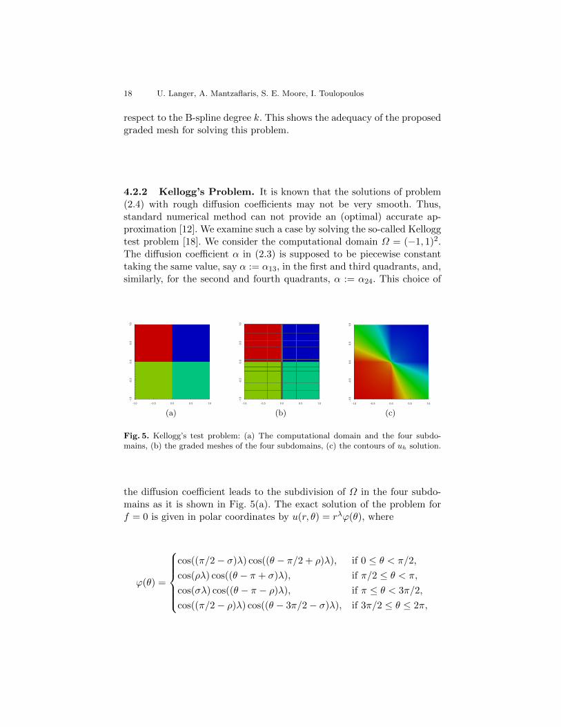
4.2.2 Kellogg’s Problem. It is known that the solutions of problem(2.4) with rough diffusion coefficients may not be very smooth. Thus,standard numerical method can not provide an (optimal) accurate ap-proximation [12]. We examine such a case by solving the so-called Kelloggtest problem [18]. We consider the computational domain Ω = (−1, 1)2.The diffusion coefficient α in (2.3) is supposed to be piecewise constanttaking the same value, say α := α13, in the first and third quadrants, and,similarly, for the second and fourth quadrants, α := α24. This choice of

(a) (b) (c)

Fig. 5. Kellogg’s test problem: (a) The computational domain and the four subdo-mains, (b) the graded meshes of the four subdomains, (c) the contours of uh solution.

the diffusion coefficient leads to the subdivision of Ω in the four subdo-mains as it is shown in Fig. 5(a). The exact solution of the problem forf = 0 is given in polar coordinates by u(r, θ) = rλϕ(θ), where

ϕ(θ) =

cos((π/2− σ)λ) cos((θ − π/2 + ρ)λ), if 0 ≤ θ < π/2,

cos(ρλ) cos((θ − π + σ)λ), if π/2 ≤ θ < π,

cos(σλ) cos((θ − π − ρ)λ), if π ≤ θ < 3π/2,

cos((π/2− ρ)λ) cos((θ − 3π/2− σ)λ), if 3π/2 ≤ θ ≤ 2π,


where the numbers λ, ρ, σ satisfy the nonlinear relations

R := α13α24

= − tan((π/2− σ)λ) cot(ρλ),1R = − tan(ρλ) cot(σλ),

R = − tan(σλ) cot((π/2− ρ)λ),

0 < λ < 2,

max0, πλ− π < 2λρ < minπλ, π,max0, π − πλ < −2λσ < minπ, 2π − λπ.

For λ = 0.4, the solution u ∈W 1.4,2(Ω), and has discontinuous deriva-tives across the interfaces. On the other hand, u ∈ W 2,1.25(Ω), and theestimates presented in Section 3.3 can be applied. We solved the problemusing B-spline spaces with degrees k = 1 and k = 2 on uniform meshes.We performed again the test using graded meshes with grading parameterchosen such that λ/µ = k, see (3.9). In Fig. 5(b), we can see the gradedmeshes of the subdomains. Fig. 5(c) shows the plot of the contours ofthe dG solution uh computed for degree k = 1 B-splines. In Table 3, wedisplay the convergence rates of the solution. We observe that, in the caseof uniform meshes, the experimental order of convergence of the methodis 0.4 which is determined by the regularity of the solution. Conversely,the rates in the right columns which correspond to the results using meshgrading tend to be optimal with respect the order of the B-spline space.A glimpse of the discrete solution uh is given in Fig. 6.


h/2s k = 1 k = 2k = 1,µ = 0.40

k = 2,µ = 0.20

Convergence rates

s = 0 - - - -s = 1 0.655814 0.591165 0.830217 0.477657s = 2 0.354865 0.355586 0.858329 1.15442s = 3 0.368103 0.378796 0.879976 1.78696s = 4 0.378375 0.385672 0.895984 1.84425s = 5 0.385464 0.390348 0.906179 1.95223

Table 3. Kellogg’s test: The convergence rates in the dG-norm ‖.‖dg(Ω).

4.3 Three dimensional examples

4.3.1 Cube with interior point singularity. This test case is in-spired by [21]. The computational domain is Ω = (−1, 1)3 which is decom-


Fig. 6. Discrete solution of Kellogg’s problem plotted over the graded mesh.

posed into 8 subdomains, see Fig. 7(a). We choose the diffusion coefficientα = 1 in the whole computational domain Ω. The solution of the problemhas a singular point at the origin of the axis and is given by u(x) = |x|λwith λ = 0.85. It is easy to show that u ∈ W l=2,2(Ω). We solved theproblem using k = 1, k = 2 and k = 3 B-spline spaces on quasi-uniformmeshes. In Fig. 7(b), we plot the contours of solution uh computed byk = 1 B-spline space. The convergence rates of the error correspondingto non-graded meshes are shown in left columns of Table 4.

(a)

0.4

0.8

1.2

Sol

0

1.6

(b)

0.4

0.8

1.2

Sol

0

1.6

(c)

Fig. 7. Cube with interior singularity: (a) the decomposition of Ω into 8 subdomainswith the graded meshes of the subdomain, (b) the contours of the solution uh, (c) thevariance of the uh contours around the singular point.

The rates are optimal for k = 1 B-spline space and sub-optimal for thetwo other B-spline spaces, as it was expected according to the regularity ofthe solution u. Note that the rates presented on the left columns in Table4 are in agreement with the estimate given in (3.7a). We have performedagain the test using grading meshes for the last two B-spline spaces. The


grading parameter µ has been chosen to be δ(l = 2, p = 2, d = 3)/µ = k,see Lemma 1 and (3.9). In Fig. 7(c), the variate of the uh contours aroundthe singular point is shown. The rates obtained on graded meshes aredisplayed in right columns of Table 4.


h/2s k = 1 k = 2 k = 3k = 1,µ = 1.0

k = 2,µ = 0.6

k = 3,µ = 0.4

Convergence rates

s = 0 - - - - - -s = 1 0.593 1.066 0.687 0.593 1.393 0.791s = 2 0.839 1.306 1.234 0.839 1.766 1.870s = 3 0.917 1.340 1.343 0.917 1.928 2.942s = 4 0.953 1.346 1.350 0.953 1.959 3.080s = 5 0.972 1.348 1.350 0.972 1.974 3.066

Table 4. Cube with interior singularity: The convergence rate of the error on uniformand graded meshes.

We can observe that the rates approach the optimal rate for bothhigh-order B-spline spaces. This numerical example demonstrates thatthe dG IgA method applied on the proposed graded meshes can exhibitoptimal convergence rates for interior singularity type problems as well.

4.3.2 Three-dimensional L-shape domain. Now the computationaldomainΩ has 3d L-shape form and is given by

((−1, 1)2 \ (−1, 0)2

)×[0, 1].

Even though the ”L-shape“ example has been mostly studied in the lit-erature in its two-dimensional set up, (see for example anisotropic 2dmeshes for IgA discretizations in [8]), we believe that it is an interestingtest case, because we will see that the graded mesh of the plane can beprolonged in a direction perpendicular to the singular edge for treatingthe boundary singularities. Note that in this three dimensional setting,the domain includes both corner and edge singularities, see Fig. 8(a).

We consider an exact solution given by u = rλ sin( θπω ), where λ = π/ωand ω = 3π/2. We set ΓD = ∂Ω. The data f and uD of (2.3) are given bythe exact solution. The computational domain Ω consists of two subdo-mains We have solved the problem using B-spline spaces of order k = 1and k = 2 using quasi-uniform and graded meshes in both subdomains.The grading parameter is defined by the relation δ(l, p, d)/µ = k. InFig. 8(b), we can see the graded meshes for µ = 0.6. The contours ofthe corresponding approximate solution uh computed for k = 1 are pre-


(a) (b)

40

80

120

Solution

0

126

(c)

Fig. 8. 3d L-shape test: (a) The domain Ω with the corners and the edge boundarysingularities, (b) The graded meshes of the two subdomain, (c) The contours of uh.

sented in Fig. 8(c). Table 5 displays the convergence rates of the error.We observe the same behavior of the rates as in the previous examples.The rates of the uniform meshes are determined by the regularity of thesolution (u ∈ W 1+λ,p=2(Ω)) for both B-spline spaces. The convergencerates corresponding to graded meshes approach the optimal value. Weremark here that the same type of graded meshes have also been used infinite element methods for approximating solutions of elliptic problems inthree-dimensional domains with edges, see [6, 5, 4].


h/2s k = 1 k = 2k = 1,µ = 0.6

k = 2,µ = 0.3

Convergence rates

s = 0 - - - -s = 1 0.645078 0.477178 0.629909 0.387338s = 2 0.650805 0.639951 0.869128 1.11198s = 3 0.642971 0.670841 0.883655 1.80531s = 4 0.644107 0.669949 0.902467 1.96533s = 5 0.648100 0.668371 0.920065 2.00296

Table 5. 3d L-shape : The convergence rates of the error with respect to the dG normon uniform and graded meshes.

4.3.3 Three-dimensional heart shaped domain. In this example,we consider an exact solution given by u = rλ sin(θπ/ω), where λ = π/ωand ω = 3π/2. We again set ΓD = ∂Ω, and the data f and uD of (2.3)are specified by the given exact solution. The computational domain Ωconsists of two subdomains. The problem is solved with B-spline spaces


of order k = 1 and k = 2 using quasi-uniform and graded meshes in bothsubdomains. The grading parameter is defined by the relation λ/µ = k.In Fig. 9(b), we can see the graded meshes for µ = 0.6. The contours ofthe corresponding approximate solution uh computed with degree k = 1is presented in Fig. 9(c).

The convergence rates of the error corresponding to the quasi-uniformmeshes are shown in left columns (without grading) of Table 6, and therates corresponding to the graded meshes are shown in the right columnsof Table 6.

(a) (b)

1000

2000

3000

Solution

0

3.32e+03

(c)

Fig. 9. 3D heart test: (a) The domain Ω with the corners and edge boundary singu-larities, (b) The graded meshes of the two subdomain, (c) The contours of uh.


h/2s k = 1 k = 2k = 1,µ = 0.6

k = 2,µ = 0.3

Convergence rates

s = 0 - - - -s = 1 0.650805 0.675611 0.686633 0.964287s = 2 0.642971 0.685756 0.846524 1.55143s = 3 0.644107 0.674337 0.902119 1.91781s = 4 0.6481 0.669817 0.925762 2.10561s = 5 0.65251 0.667968 0.94134 2.09457

Table 6. 3d Heart : The convergence rates of the error with respect to the dG normon uniform and graded meshes.

5 Conclusion

We have presented mesh grading techniques for dG IgA discretizions ofelliptic boundary value problems in the presence of so-called singular


points. Based on the a priori or a posteriori knowledge of the behaviour ofthe exact solution around the singular points, we pre-defined the gradingof the mesh without increasing the knots but performing a relocation.The grading refinement has a subdomain (patch) character in order to fitwell into the IgA framework. Optimal error estimates of the multipatchdG IgA method have been shown when it is used on the graded meshesproposed. The theoretical results have been confirmed by a number oftwo- and three-dimensional test problems with known exact solutions.

Acknowledgments

This research was supported by the National Research Network NFNS117-03 “Geometry + Simulation” of the Austrian Science Fund (FWF).

References

1. R. A. Adams and J. J. F. Fournier. Sobolev Spaces, volume 140 of Pure and AppliedMathematics. ACADEMIC PRESS-imprint Elsevier Science, second edition, 2003.

2. T. Apel. Interpolation of non-smooth functions on anisotropic finite elementmeshes. M2AN, 33(6):1149–1185, 1999.

3. T. Apel and B. Heinrich. Mesh refinement and windowing near edges for someelliptic problem. SIAM J. Numer. Anal., 31(3):695–708, 1994.

4. T. Apel and B. Heinrich. The finite element method with anisotropic mesh gradingfor elliptic problems in domains with corner and edges. SIAM J. Numer. Anal.,31(3):695–708, 1998.

5. T. Apel and F. Milde. Comparison of several mesh refinement strategies nearedges. Comput. Methods Appl. Mech. Eng., 12:373–381, 1996.

6. T. Apel, A.-M. Sandig, and J. R. Whiteman. Graded mesh refinement and errorestimates for finite element solutions of elliptic boundary value problems in non-smooth domains. Math. Methods Appl. Sci., 19(30):63–85, 1996.

7. Y. Bazilevs, L. Beirao da Veiga, J.A. Cottrell, T.J.R. Hughes, and G. Sangalli.Isogeometric analysis: Approximation, stability and error estimates for h-refinedmeshes. M3AS, 16(07):1031–1090, 2006.

8. L. Beirao da Veiga, D. Cho, and G. Sangalli. Anisotropic NURBS approximationin isogeometric analysis. Comp. Methods in Appl. Mech and Engrg, 209212(0):1 –11, 2012.

9. J. A. Cotrell, T. J. R. Hughes, and Y. Bazilevs. Isogeometric Analysis, TowardIntegration of CAD and FEA. John Wiley and Sons, 2009.

10. Daniele A. Di Pietro and Alexandre Ern. Mathematical Aspects of DiscontinuousGalerkin Methods, volume 69 of Mathematiques et Applications. Springer-Verlag,Heidelberg, Dordrecht, London, New York, 2012.

11. M. Dryja. On discontinuous Galerkin methods for elliptic problems with discon-tinuous coeffcients. Comput. Methods Appl. Math., 3:76–85, 2003.

12. S. R. Falkand and J. E. Osborn. Remarks on mixed finite element methods forproblems with rough coefficients. Math. Comp., 62(205):1–19, 1994.


13. M. Feistauer and A.-M. Sandig. Graded mesh refinement and error estimates ofhigher order for dgfe solutions of elliptic boundary value problems in polygons.Numer. Methods Partial Diff. Equations, 28(4):1124–1151, 2012.

14. P. Grisvard. Elliptic problems in nonsmooth domains. Monographs and studies inmathematics. Pitman Advanced Pub. Program, 1985.

15. P. Grisvard. Singularities in Boundary Value Problems. Recherches enmathematiques appliquees. Masson, 1992.

16. T.J.R. Hughes, J.A. Cottrell, and Y. Bazilevs. Isogeometric analysis: CAD, finiteelements, NURBS, exact geometry and mesh refinement. Comput. Methods Appl.Mech. Engrg., 194:4135–4195, 2005.

17. J. W. Jeong, H. S. Oh, S. K., and H. Kim. Mapping techniques for isogeomet-ric analysis of elliptic boundary value problems containing singularities. Comp.Methods in Appl. Mech and Engrg, 254(0):334 – 352, 2013.

18. R. B. Kellogg. On the Poisson equation with intersecting interfaces. Appl. Anal.,4:101–129, 1975.

19. V. A. Kondrat’ev. Boundary value problems for elliptic equations in domains withconical or angular points. Transl. Moscow Math. Soc., 16:227–313, 1967.

20. V.A. Kozlov, V. G. Maz’ya, and J. Rossmann. Spectral Problems Associated withCorner Singularities of Solutions to Elliptic Equations, volume 85 of MathematicalSurveys and Monographs. Americanb Mathematical Society, Rhode Issland, USA,2001.

21. D. Kroner, M. Ruzicka, and I. Toulopoulos. Numerical solutions of systems with(p, δ)-structure using local discontinuous Galerkin finite element methods. Int. J.Numer. Methods Fluids, 2014.

22. U. Langer, A. Mantzaflaris, S.E. Moore, and I. Toulopoulos. Multipatch discon-tinuous Galerkin Isogeometric Analysis. RICAM Reports 2014-18, Johann RadonInstitute for Computational and Applied Mathematics, Austrian Academy of Sci-ences, Linz, 2014. http://arxiv.org/abs/1411.2478v1.

23. U. Langer and S.E. Moore. Discontinuous Galerkin isogeometric analysis of ellipticPDEs on surfaces. NFN Technical Report 12, Johannes Kepler University Linz,NFN Geometry and Simulation, Linz, 2014. http://arxiv.org/abs/1402.1185 andaccepted for publication in the DD22 proceedings.

24. U. Langer and I. Toulopoulos. Analysis of multipatch discontinuous Galerkin IgAapproximations to elliptic boundary value problems. RICAM Reports 2014-08,Johann Radon Institute for Computational and Applied Mathematics, AustrianAcademy of Sciences, Linz, 2014. http://arxiv.org/abs/1408.0182.

25. L.A. Oganesjan and L.A. Ruchovetz. Variational Difference Methods for the So-lution of Elliptic Equations. Isdatelstvo Akademi Nank Armjanskoj SSR, Erevan,1979. (in Russian).

26. H. S. Oh, H. Kim, and J. W. Jeong. Enriched isogeometric analysis of ellipticboundary value problems in domains with cracks and/or corners. Int. J. Numer.Meth. Engn, 97(3):149–180, 2014.

27. B. Riviere. Discontinuous Galerkin Methods for Solving Elliptic and ParabolicEquations: Theory and Implementation. SIAM, Philadelphia, 2008.

28. L. L. Schumaker. Spline Functions: Basic Theory. Cambridge, University Press,3rd edition, 2007.

29. G. Strang and G. Fix. An Analysis of the Finite Element Method. Prentice-Hall.Englewood Cliffs, N.J., 1973.

mesh grading in isogeometric analysis - inria

Documents