piecewise polynomial interpolationhermite interpolation 10 we can impose smoothness at the nodes to...

Piecewise Polynomial Interpolation

1

Piecewise linear interpolation

2

Suppose we have data point (xk, yk), k = 0, 1, . . . N .

A piecewise linear polynomial that interpolates these

points is given by

p(x) = pk(x), x 2 [xk, xk+1]

where the polynomials pk(x) can be written as

pk(x) = a1(x� xk) + a0, k = 1, 2, . . . N � 1

At this point, we could easily compute the coe�cients

a = [a1, a0], but let’s go through a more general proce-

dure that we can use for higher order piecewise poly-

nomials.


3

We can write this as a function of a local variable t which measures

the distance along the interval.

t =

x� xk

xk+1 � xkx = hkt+ xk

where hk = xk+1 � xk. Then, for 0 t 1, we have

pk(x) = epk(t) = ea1t+ ea0

(xk, yk)

(xk+1, yk+1)

t = 0

t = 1

0 < t < 1

epk(0) = yk

epk(1) = yk+1

Constraints to impose


4

This leads to a linear system

0 1

1 1

� ea1ea0

�=

ykyk+1

�

which we write as Aea = p. To solve for the coe�cients,

we use the matrix co-factor C to get A�1

A�1=

CT

det(A)

=

1

det(A)

1 �1

�1 0

�

We have det(A) = �1, and so

ea = �CTp


5

To see what epk(t) looks like, we let q(t) = [t, 1] andwrite

epk(t) =

eaTq(t)= �pTCq(t)

= �⇥yk yk+1

⇤T

1 �1

�1 0

� t1

�

The advantage of this form is that we can clearly see

how the polynomial epk(t) depends on our data yk and

yk+1 :

epk(t) = (1� t)yk + tyk+1


6

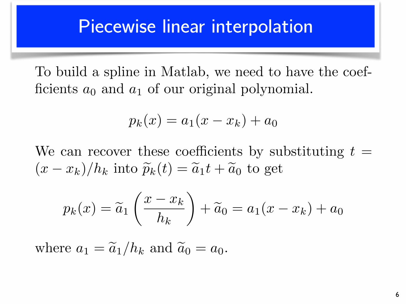
To build a spline in Matlab, we need to have the coef-

ficients a0 and a1 of our original polynomial.

pk(x) = a1(x� xk) + a0

We can recover these coe�cients by substituting t =

(x� xk)/hk into epk(t) = ea1t+ ea0 to get

pk(x) = ea1✓x� xk

hk

◆+ ea0 = a1(x� xk) + a0

where a1 = ea1/hk and ea0 = a0.


7

These are exactly the coefficients that Matlab needs to build a spline using ‘mkpp’.

We can also write a = [a1, a0] using

a = �pTCS = �⇥yk yk+1

⇤ 1 �1

�1 0

� 1/hk 0

0 1

�

=

" yk+1 � ykhkyk

#

function pp_linear = build_linear_spline(xdata,ydata)N = length(xdata)-1;h = diff(xdata); %(x1-x0, x2-x1, x3-x2,...)C = [1 -1; -1 0];for k = 1:N, p = [ydata(k); ydata(k+1)]; S = diag([1./h(k) 1]); coeffs(k,:) = -p'*C*S;endpp_linear = mkpp(xdata,coeffs);end


8

(x5, y5)

(x0, y0)

(x2, y2)

(x4, y4)


9

Can we come design a method that matches derivatives at the nodes as well?

Piecewise linear interpolation has these properties

• Continuous at nodes (xk, yk).

• Derivatives are not continuous (the function is

not smooth!)

Hermite interpolation

10

We can impose smoothness at the nodes to get a nicer looking curve. Suppose we match the function values and derivatives.

p(xk) = yk

p

0(xk) = dk

p(xk+1) = yk+1

p

0(xk+1) = dk+1

Four conditions allow us to find the four coefficients of a cubic polynomial

This approach assumes that we have derivatives dk at each of the nodes xk.

pk(x) = a3(x� xk)3 + a2(x� xk)

2 + a1(x� xk) + a0


11

As before, define

t =

x� xk

xk+1 � xk, ! x = hkt+ xk

where hk = xk+1 � xk. Then, for 0 t 1, we have

pk(x) ⌘ epk(t) = ea3t3 + ea2t2 + ea1t+ ea0

and our four conditions become

epk(0) = yk epk(1) = yk+1

ep0k(0) = dkhk ep0k(1) = dk+1hk


12

This leads to the following linear system for the coe�cients ean :

We write the above system as Aea = p. To invert A, we use the

co-factor matrix C to get

A�1=

CT

det(A)

See Strang’s Introduction to Linear Algebra for more information on

the co-factor formula for the matrix inverse.


13

We can then write epk(t) as

epk(t) = eaTq(t) = �pTCq(t)

where q(t) = [t3, t2, t, 1]T and we have used the fact that det(A) = �1.

Computing C, we get

epk(t) = �⇥yk yk+1 dkhk dk+1hk

⇤T

2

664

�2 3 0 �1

2 �3 0 0

�1 2 �1 0

�1 1 0 0

3

775

2

664

t3

t2

t1

3

775

which leads to a formula that clearly shows how the polynomial de-

pends on our data yk, yk+1, dk and dk+1:

epk(t) =

⇥1� t2(3� 2t)

⇤yk +

⇥t2(3� 2t)

⇤yk+1

+

⇥t(t� 1)

2⇤hkdk +

⇥t2(t� 1)

⇤hkdk+1

Piecewise Cubic Hermite Interpolating Polynomial (PCHIP)

14

epk(t) =

⇥1� t

2(3� 2t)

⇤yk +

⇥t

2(3� 2t)

⇤yk+1

+

⇥t(t� 1)

2⇤hkdk +

⇥t

2(t� 1)

⇤hkdk+1

If we substitute t = (x � xk)/hk, we can recover our original poly-

nomial in x :

pk(x) = a3(x� xk)3+ a2(x� xk)

2+ a1(x� xk) + a0

where an = ean/hnk . We can write these coe�cients as

a = �pTCS

where S = diag(h

�3k , h

�2k , h

�1k , 1), p = [yk, yk+1, dkhk, dk+1hk], and

C is the co-factor matrix of our original coe�cient matrix A.

These are exactly the coefficients that Matlab needs to build a spline using ‘mkpp’.

The derivatives?

15

Where do we get the derivatives dk from?

• If we know f(x), we can set dk = f

0(xk).

• We can approximate derivatives using data (xk, yk).

dk = G (�k�1, �k) , �k =yk+1 � yk

hk

where, for example, we could take G(a, b) = a+b2 , G(a, b) =

a, G(a, b) = b or some other reasonable function. Matlab’sPCHIP chooses derivatives to avoid introducing new extremain the spline.

• We can impose additional smoothness conditions and solveimplicitly for the derivatives.

Derivatives?

16

Given data points (x0, y0), . . . , (xN , yN ), impose continuity in the

second derivative at the interior nodes,

p

00k(xk+1) = p

00k+1(xk+1), k = 1, 2, . . . N � 1.

This leads to a tridiagonal system for the derivatives at internal

nodes (”knots”) d1, d2, d3, . . . , dN�1.

To get equations for the end point derivatives, we will need to

to impose additional conditions at the endpoints.


17

The entries in the tridiagonal system can be found by considering the polynomials

as functions of t :

p

00k�1(x) =

1

h

2k�1

p̃

00k�1(t), x = hk�1t+ xk�1

Transforming the equations equating second derivatives at knots, we obtain

1

h

2k�1

p̃

00k�1(1) =

1

h

2k

p̃

00k(0), k = 1, 2, 3, . . . N � 1

Using p̃

00k(t) = �pT

Cq00(t), we get

6

h

2k�1

yk�1 �6

h

2k�1

yk +2

hk�1dk�1 +

4

hk�1dk =

6

h

2k

yk �6

h

2k

yk+1 +2

hkdk +

4

hkdk+1

or

1

hk�1dk�1 +

✓1

hk�1+

1

hk

◆dk +

1

hkdk+1 =

3

h

2k�1

(yk � yk�1) +3

h

2k

(yk+1 � yk)

for k = 1, 2, 3, . . . , N � 1. This leads to a tridiagonal system for the unknown

derivatives dk.


18

We can combine all equations into an (N �1)⇥ (N +1) ”augmented” tridiagonal

system A0d = b, or

2

666664

u0 u0 + u1 u1

u1 u1 + u2 u2

u2 u2 + u3 u3

.

.

.

.

.

.

.

.

.

uN�2 uN�2 + uN�1 uN�1

3

777775

2

666664

d0d1.

.

.

dN�1

dN

3

777775=

2

666664

b1.

.

.

.

.

.

bN�1

3

777775

where the matrix A0

A0=

⇥u0 A uN

⇤

and

ui =1

hi, k = 0, 1, 2, . . . , N � 1

bi = 3u2i�1(yi � yi�1) + 3u2

i (yi+1 � yi), k = 1, 2, 3, . . . , N � 1.

We can write this as a square tridiagonal system

Ad = b� d0u0 � dNuN

where u0 and uN are the first and last columns ofA0above, and d = (d1, d2, . . . , dN�1)


19

We solve for the unknown derivatives d0, d1, d2, . . . , dN in three steps.

1. Solve dH = A�1b.

2. Solve

Ad0 = u0

AdN = uN

for vectors d0 and dN .

3. Solve

F(d0, dN ) =

a11 a12a21 a22

� d0dN

�+

F0

FN

�= 0

for scalars d0, dN so that so that ”endpoint” conditions (to be determined)

are satisfied. Coe�cients for the above system depend on choice of endpoint

conditions.

All unknown derivatives are then given by

d =

�d0, dH � d0d0 � dNdN , dN

End conditions?

20

There are several additional conditions we can impose to solve for the endpoint

derivatives.

• Clamp derivative values d0 and dN to fixed values,

• Fit a cubic through first (last) four points and set d0 (dN ) to the derivative

of this polynomial at x0 (xN ).

• Impose continuity of the third derivative at x1 (xN�1). This is the ”not-a-

knot” condition, since we now have a single cubic polynomial over [x0, x2]

and [xN�2, xN ], e↵ectively eliminating the second (and second to last) node

(or ”knot”).

• For a periodic spline, match first and second derivatives between x0 and

xN .

• Impose the ’natural’ endpoint conditions, i.e. second derivative equal to 0.

Each of these can be represented as a 2⇥ 2 system of the form

F(d0, dN ) =

a11 a12

a21 a22

� d0

dN

�+

F0

FN

�= 0

After determining coe�cients, we can then solve for d0 and dN .

Cubic spline

21

Periodic spline

22

piecewise polynomial interpolationhermite interpolation 10 we can impose smoothness at the nodes to...

Documents