pico:a domain-specific language for data analytics pipelinestremblay/misale.pdf · consigli per la...
TRANSCRIPT

University of Torino
Doctoral School on Scienceand High Technology
Computer Science Department
Doctoral Thesis
PiCo:A Domain-Specific Language for
Data Analytics Pipelines
Author:Claudia Misale
Cycle XVIII
Supervisor:Prof. Marco Aldinucci
Co-Supervisor:Prof. Guy Tremblay
A thesis submitted in fulfillment of the requirementsfor the degree of Doctor of Philosophy

ii
“Simplicity is a great virtue but it requires hard work to achieve itand education to appreciate it.And to make matters worse: complexity sells better. ”
Edsger W. Dijkstra, “On the nature of Computing Science”
Marktoberdorf, 10 August 1984

iii
UNIVERSITY OF TORINO
Abstract
Computer Science Department
Doctor of Philosophy
PiCo:A Domain-Specific Language for Data Analytics Pipelines
by Claudia Misale
In the world of Big Data analytics, there is a series of tools aiming at simplifyingprogramming applications to be executed on clusters. Although each tool claims toprovide better programming, data and execution models—for which only informal(and often confusing) semantics is generally provided—all share a common under-lying model, namely, the Dataflow model. Using this model as a starting point, it ispossible to categorize and analyze almost all aspects about Big Data analytics toolsfrom a high level perspective. This analysis can be considered as a first step towarda formal model to be exploited in the design of a (new) framework for Big Dataanalytics. By putting clear separations between all levels of abstraction (i.e., fromthe runtime to the user API), it is easier for a programmer or software designerto avoid mixing low level with high level aspects, as we are often used to see instate-of-the-art Big Data analytics frameworks.
From the user-level perspective, we think that a clearer and simple semantics ispreferable, together with a strong separation of concerns. For this reason, we usethe Dataflow model as a starting point to build a programming environment witha simplified programming model implemented as a Domain-Specific Language, thatis on top of a stack of layers that build a prototypical framework for Big Dataanalytics.
The contribution of this thesis is twofold: first, we show that the proposed modelis (at least) as general as existing batch and streaming frameworks (e.g., Spark,Flink, Storm, Google Dataflow), thus making it easier to understand high-leveldata-processing applications written in such frameworks. As result of this analysis,we provide a layered model that can represent tools and applications following theDataflow paradigm and we show how the analyzed tools fit in each level.
Second, we propose a programming environment based on such layered model in theform of a Domain-Specific Language (DSL) for processing data collections, calledPiCo (Pipeline Composition). The main entity of this programming model isthe Pipeline, basically a DAG-composition of processing elements. This model isintended to give the user an unique interface for both stream and batch processing,hiding completely data management and focusing only on operations, which arerepresented by Pipeline stages. Our DSL will be built on top of the FastFlowlibrary, exploiting both shared and distributed parallelism, and implemented inC++11/14 with the aim of porting C++ into the Big Data world.


v
AcknowledgementsQuesti quattro anni sono stati veramente brevi. Praticamente non me ne sonoaccorta. Ho imparato tante cose, molte ancora non ho capito come si fanno (adesempio non so fare le revisioni in maniera educata ed elegante, non ho imparatoa parlare in pubblico, non so riassumere i meeting..) e faccio ancora arrabbiaretantissimo il mio supervisore, il Professor Marco Aldinucci. A lui, infatti, diresemplicemente “grazie” non e abbastanza. Specie per la pazienza che ha avuto conme, da tutti i punti di vista.
These four years were really short. I did not notice they are gone. I learned a lot,I still do not understand how to do a lot of things (for instance I am not able toreview papers in a polite and elegant way, I did not learn to talk in public, I am notable to summarize meetings..) and I still make my supervisor very angry with me,Professor Marco Aldinucci. It is not enough to say “thank you” to him. Especiallyfor the patience he had with me, from all points of view.
Sono arrivata a Torino senza conoscerlo, chiedendogli di essere il mio supervisoreper il dottorato. Non potevo fare scelta migliore. Tutto quello che so lo devo a lui.Le ore passate ad ascoltarlo spiegarmi i mille aspetti di quest’area di ricerca (anchese per lui, di aspetti, ce ne sono sempre e solo due), mi hanno aperto la mente emi hanno formato tantissimo, anche se ancora ho tutto da imparare. Quattro anni,infatti, non bastano. Mi ha sempre spronato a fare meglio, a guardare dentro lecose, e cerchero di portarmi dietro i suoi insegnamenti ovunque la vita mi portera.Inoltre la sua simpatia e i suoi modi di fare, sono stati ottimi compagni in questianni di dottorato. Sı, anche gli insulti lo sono stati! Grazie, theboss. Di cuore.
I arrived in Turin without knowing that much about Prof. Aldinucci and I asked himto be my supervisor. I could not make a better choice. Everything I know is thanks tohim. I spent a lot of hours listening to him explaining all aspects about this researcharea (even if, from his point of view, there are always only two aspects), this openedmy mind and made me grow up a lot, even if I still have to learn. Four years arenot enough, actually. He always pushed me to do my best, to look inside things, andI will always try to bring his teachings with me, wherever I will go. Furthermore,his pleasantness and his way to do things, have been perfect companionship in theseyears. Thank you, theboss. Thank you so much.
Ci sono alcune persone che voglio ringraziare, perche tanto mi hanno dato e sarosempre in debito con loro per questo.
There are a few people I want to thank, because they gave me so much and I willalways be in debt with them.
Vorrei iniziare con il mio co-supervisore, il Professor Guy Tremblay. Grazie diavermi seguito e di avermi aiutato cosı tanto nella stesura della tesi e nel capiretanti argomenti che, per entrambi, erano nuovi: la tua grande esperienza e statailluminante, sei stato una guida importantissima. Grazie ancor di piu per i tanticonsigli per la presentazione che mi hai dato, ho cercato di seguirli al meglio e sperodi esserne stata all’altezza.
I would like to start with my co-supervisor, professor Guy Tremblay. Thank you somuch for helping me so much while writing this thesis and thank you for helpingme in understanding topics that, for both, were new: your great experience has beenenlightening, you have been a very important guide. Thank you even more for allthe advices about the presentation, I tried to follow all of them the best I can do andI hope I have been able to do that.
Vorrei ringraziare i revisori per il lavoro di revisione che hanno fatto: i loro com-menti sono stati preziosissimi e molto dettagliati. Mi hanno permesso di migliorareil manoscritto e soprattutto di rivedere molti aspetti che l’inesperienza non mi per-mette ancora di vedere.

vi
I would like to thank reviewers for the great job they did, their impressive knowledgeand experience, and the time the dedicated to my work: their comments have beenprecious and very detailed. Their advices made me improve the manuscript and,mostly, to review a lot of aspects that the inexperience makes me not able to seethem yet.
Un profondo grazie va ai miei colleghi: una cricca di persone uniche con cui hocondiviso tanto e tanto mi hanno dato. Le nostre serate “non facciamo tardi” chefinivano alle 4 o 5 del mattino, le mangiate, le uscite, i giochi, i mille discorsi, leGossip Girlz.. Grazie di tutto cio che mi avete dato.
Grazie a Caterina, la mia secolare amica. Tu sai tutto di me, che altro ti devo dire.Siamo cresciute insieme nei cinque anni di universita all’UniCal in cui ne abbiamocombinate tante e mi hai assistito durante questi anni: sei anche tu una colonnaportante di questo dottorato e una portante nella mia vita.
Quasi tutte le pause pranzo del mio dottorato le ho trascorse in palestra a “pic-chiare la gente”, come dicono i miei colleghi. Le lezioni di kick-boxing/muay-thaisono state assolutamente una droga e a renderle tali sono state innanzitutto le per-sone che ho conosciuto lı. Grazie al Maestro Beppe e ai ragazzi, ho imparato adapprezzare questo magnifico sport fatto di disciplina, rispetto, autocontrollo, che miha permesso di spingermi oltre i cio che pensavo fossero i miei limiti fisici e mentali.Grazie, Maestro, per avermi fatto scoprire un lato di me a me sconosciuto e graziedella persona e amico che sei. Grazie a tutti i miei “amici delle botte”, grazie dellebotte che mi avete dato, della perfetta compagnia che siete sia in palestra che fuori,per avermi aiutato a scaricare l’ansia accumulata ogni giorno.
Grazie a Roberta, la mia amica di botte numero uno in assoluto. Abbiamo condivisotanto in palestra e siamo cresciute insieme, mi hai fatto crescere e mi hai insegnatotanto. Soprattutto, hai ascoltato e sopportato tutti i miei sfoghi e le mie frustrazionida dottoranda. Mai ti ringraziero abbastanza.
E infine, i pezzi grossi. La mia famiglia, a cui tutto devo. Soprattutto per lapazienza che avete avuto con me: so che e stata dura, infatti vi chiedo scusa perquesto. Grazie per l’avermi sempre appoggiato in tutte le mie scelte e per avermipermesso di raggiungere questo traguardo. Vorrei sempre rendervi orgogliosi di mee spero che questo dottorato mi aiuti in questo obiettivo. Perche siete il mio esempiodi correttezza e forza.
Maurizio. Ti ho conosciuto durante il nostro dottorato, sei diventato parte dellamia vita dal primo istante. Abbiamo condiviso questo percorso insieme: i momentibelli, quelli un po’ critici, la fatica mentale e fisica. La tua intelligenza e le tueintuizioni mi hanno sempre affascinato e ispirato. Spero sarai orgoglioso, almenoun po’, di me alla fine di questa storia. Lo sai che.

vii
Contents
Abstract iii
Acknowledgements v
1 Introduction 11.1 Results and Contributions . . . . . . . . . . . . . . . . . . . . . . . . 11.2 Limitations and Future Work . . . . . . . . . . . . . . . . . . . . . . 41.3 Plan of the Thesis . . . . . . . . . . . . . . . . . . . . . . . . . . . . 51.4 List of Papers . . . . . . . . . . . . . . . . . . . . . . . . . . . . . . . 51.5 Funding . . . . . . . . . . . . . . . . . . . . . . . . . . . . . . . . . . 7
2 Technical Background 92.1 Parallel Computing . . . . . . . . . . . . . . . . . . . . . . . . . . . . 92.2 Platforms . . . . . . . . . . . . . . . . . . . . . . . . . . . . . . . . . 9
2.2.1 SIMD computers . . . . . . . . . . . . . . . . . . . . . . . . . 10Symmetric shared-memory multiprocessors . . . . . . . . . . 10Memory consistency model . . . . . . . . . . . . . . . . . . . 11Cache coherence and false sharing . . . . . . . . . . . . . . . 12
2.2.2 Manycore processors . . . . . . . . . . . . . . . . . . . . . . . 122.2.3 Distributed Systems, Clusters and Clouds . . . . . . . . . . . 14
2.3 Parallel Programming Models . . . . . . . . . . . . . . . . . . . . . . 142.3.1 Types of parallelism . . . . . . . . . . . . . . . . . . . . . . . 15
Data parallelism . . . . . . . . . . . . . . . . . . . . . . . . . 16Map . . . . . . . . . . . . . . . . . . . . . . . . . . . . . . . . 16Reduce . . . . . . . . . . . . . . . . . . . . . . . . . . . . . . 17
2.3.2 The Dataflow Model . . . . . . . . . . . . . . . . . . . . . . . 18Actors . . . . . . . . . . . . . . . . . . . . . . . . . . . . . . . 18Input channels . . . . . . . . . . . . . . . . . . . . . . . . . . 19Output channels . . . . . . . . . . . . . . . . . . . . . . . . . 19Stateful actors . . . . . . . . . . . . . . . . . . . . . . . . . . 19
2.3.3 Low-level approaches . . . . . . . . . . . . . . . . . . . . . . . 192.3.4 High-level approaches . . . . . . . . . . . . . . . . . . . . . . 212.3.5 Skeleton-based approaches . . . . . . . . . . . . . . . . . . . . 22
Literature review of skeleton-based approaches . . . . . . . . 222.3.6 Skeletons for stream parallelism . . . . . . . . . . . . . . . . . 23
2.4 Programming multicore clusters . . . . . . . . . . . . . . . . . . . . . 252.4.1 FastFlow . . . . . . . . . . . . . . . . . . . . . . . . . . . . . 25
Distributed FastFlow . . . . . . . . . . . . . . . . . . . . . . . 282.5 Summary . . . . . . . . . . . . . . . . . . . . . . . . . . . . . . . . . 29
3 Overview of Big Data Analytics Tools 313.1 A Definition for Big Data . . . . . . . . . . . . . . . . . . . . . . . . 313.2 Big Data Management . . . . . . . . . . . . . . . . . . . . . . . . . . 323.3 Tools for Big Data Analytics . . . . . . . . . . . . . . . . . . . . . . 33
3.3.1 Google MapReduce . . . . . . . . . . . . . . . . . . . . . . . . 33The five steps of a MapReduce job . . . . . . . . . . . . . . . 34
3.3.2 Microsoft Dryad . . . . . . . . . . . . . . . . . . . . . . . . . 36A Dryad application DAG . . . . . . . . . . . . . . . . . . . . 36
3.3.3 Microsoft Naiad . . . . . . . . . . . . . . . . . . . . . . . . . 37

viii
Timely Dataflow and Naiad programming model . . . . . . . 373.3.4 Apache Spark . . . . . . . . . . . . . . . . . . . . . . . . . . . 38
Resilient Distributed Datasets . . . . . . . . . . . . . . . . . . 39Spark Streaming . . . . . . . . . . . . . . . . . . . . . . . . . 40
3.3.5 Apache Flink . . . . . . . . . . . . . . . . . . . . . . . . . . . 41Flink Programming and Execution Model . . . . . . . . . . . 41
3.3.6 Apache Storm . . . . . . . . . . . . . . . . . . . . . . . . . . 42Tasks and Grouping . . . . . . . . . . . . . . . . . . . . . . . 43
3.3.7 FlumeJava . . . . . . . . . . . . . . . . . . . . . . . . . . . . 44Data Model and Transformations . . . . . . . . . . . . . . . . 44
3.3.8 Google Dataflow . . . . . . . . . . . . . . . . . . . . . . . . . 45Data Model and Transformations . . . . . . . . . . . . . . . . 46
3.3.9 Thrill . . . . . . . . . . . . . . . . . . . . . . . . . . . . . . . 47Distributed Immutable Arrays . . . . . . . . . . . . . . . . . 48
3.3.10 Kafka . . . . . . . . . . . . . . . . . . . . . . . . . . . . . . . 49Producer-Consumer Distributed Coordination . . . . . . . . . 49
3.3.11 Google TensorFlow . . . . . . . . . . . . . . . . . . . . . . . . 49A TensorFlow application . . . . . . . . . . . . . . . . . . . . 50
3.3.12 Machine Learning and Deep Learning Frameworks . . . . . . 513.4 Fault Tolerance . . . . . . . . . . . . . . . . . . . . . . . . . . . . . . 513.5 Summary . . . . . . . . . . . . . . . . . . . . . . . . . . . . . . . . . 52
4 High-Level Model for Big Data Frameworks 534.1 The Dataflow Layered Model . . . . . . . . . . . . . . . . . . . . . . 53
4.1.1 The Dataflow Stack . . . . . . . . . . . . . . . . . . . . . . . 544.2 Programming Models . . . . . . . . . . . . . . . . . . . . . . . . . . . 54
4.2.1 Declarative Data Processing . . . . . . . . . . . . . . . . . . . 554.2.2 Topological Data Processing . . . . . . . . . . . . . . . . . . . 564.2.3 State, Windowing and Iterative Computations . . . . . . . . 56
4.3 Program Semantics Dataflow . . . . . . . . . . . . . . . . . . . . . . 584.3.1 Semantic Dataflow Graphs . . . . . . . . . . . . . . . . . . . 584.3.2 Tokens and Actors Semantics . . . . . . . . . . . . . . . . . . 594.3.3 Semantics of State, Windowing and Iterations . . . . . . . . . 60
4.4 Parallel Execution Dataflow . . . . . . . . . . . . . . . . . . . . . . . 604.5 Execution Models . . . . . . . . . . . . . . . . . . . . . . . . . . . . . 64
4.5.1 Scheduling-based Execution . . . . . . . . . . . . . . . . . . . 644.5.2 Process-based Execution . . . . . . . . . . . . . . . . . . . . . 66
4.6 Limitations of the Dataflow Model . . . . . . . . . . . . . . . . . . . 664.7 Summary . . . . . . . . . . . . . . . . . . . . . . . . . . . . . . . . . 67
5 PiCo Programming Model 695.1 Syntax . . . . . . . . . . . . . . . . . . . . . . . . . . . . . . . . . . . 69
5.1.1 Pipelines . . . . . . . . . . . . . . . . . . . . . . . . . . . . . 715.1.2 Operators . . . . . . . . . . . . . . . . . . . . . . . . . . . . . 71
Data-Parallel Operators . . . . . . . . . . . . . . . . . . . . . 72Pairing . . . . . . . . . . . . . . . . . . . . . . . . . . . . . . 73Sources and Sinks . . . . . . . . . . . . . . . . . . . . . . . . 73Windowing . . . . . . . . . . . . . . . . . . . . . . . . . . . . 74Partitioning . . . . . . . . . . . . . . . . . . . . . . . . . . . . 74
5.1.3 Running Example: The word-count Pipeline . . . . . . . . 755.2 Type System . . . . . . . . . . . . . . . . . . . . . . . . . . . . . . . 75
5.2.1 Collection Types . . . . . . . . . . . . . . . . . . . . . . . . . 755.2.2 Operator Types . . . . . . . . . . . . . . . . . . . . . . . . . . 765.2.3 Pipeline Types . . . . . . . . . . . . . . . . . . . . . . . . . . 77
5.3 Semantics . . . . . . . . . . . . . . . . . . . . . . . . . . . . . . . . . 785.3.1 Semantic Collections . . . . . . . . . . . . . . . . . . . . . . . 78
Partitioned Collections . . . . . . . . . . . . . . . . . . . . . . 79Windowed Collections . . . . . . . . . . . . . . . . . . . . . . 79

ix
5.3.2 Semantic Operators . . . . . . . . . . . . . . . . . . . . . . . 80Semantic Core Operators . . . . . . . . . . . . . . . . . . . . 80Semantic Decomposition . . . . . . . . . . . . . . . . . . . . . 81Unbounded Operators . . . . . . . . . . . . . . . . . . . . . . 82Semantic Sources and Sinks . . . . . . . . . . . . . . . . . . . 82
5.3.3 Semantic Pipelines . . . . . . . . . . . . . . . . . . . . . . . . 825.4 Programming Model Expressiveness . . . . . . . . . . . . . . . . . . 84
5.4.1 Use Cases: Stock Market . . . . . . . . . . . . . . . . . . . . 845.5 Summary . . . . . . . . . . . . . . . . . . . . . . . . . . . . . . . . . 86
6 PiCo Parallel Execution Graph 876.1 Compilation . . . . . . . . . . . . . . . . . . . . . . . . . . . . . . . . 87
6.1.1 Operators . . . . . . . . . . . . . . . . . . . . . . . . . . . . . 89Fine-grained PE graphs . . . . . . . . . . . . . . . . . . . . . 90Batching PE graphs . . . . . . . . . . . . . . . . . . . . . . . 91Compilation environments . . . . . . . . . . . . . . . . . . . . 92
6.1.2 Pipelines . . . . . . . . . . . . . . . . . . . . . . . . . . . . . 92Merging Pipelines . . . . . . . . . . . . . . . . . . . . . . . . 93Connecting Pipelines . . . . . . . . . . . . . . . . . . . . . . . 93
6.2 Compilation optimizations . . . . . . . . . . . . . . . . . . . . . . . . 946.2.1 Composition and Shuffle . . . . . . . . . . . . . . . . . . . . . 946.2.2 Common patterns . . . . . . . . . . . . . . . . . . . . . . . . 946.2.3 Operators compositions . . . . . . . . . . . . . . . . . . . . . 96
Composition of map and flatmap . . . . . . . . . . . . . . . . 96Composition of map and reduce . . . . . . . . . . . . . . . . 97Composition of map and p-reduce . . . . . . . . . . . . . . . 98Composition of map and w-reduce . . . . . . . . . . . . . . . 99Composition of map and w-p-reduce . . . . . . . . . . . . . . 100
6.3 Stream Processing . . . . . . . . . . . . . . . . . . . . . . . . . . . . 1016.4 Summary . . . . . . . . . . . . . . . . . . . . . . . . . . . . . . . . . 101
7 PiCo API and Implementation 1037.1 C++ API . . . . . . . . . . . . . . . . . . . . . . . . . . . . . . . . . 103
7.1.1 Pipe . . . . . . . . . . . . . . . . . . . . . . . . . . . . . . . . 1047.1.2 Operators . . . . . . . . . . . . . . . . . . . . . . . . . . . . . 105
The map family . . . . . . . . . . . . . . . . . . . . . . . . . . 106The combine family . . . . . . . . . . . . . . . . . . . . . . . 107Sources and Sinks . . . . . . . . . . . . . . . . . . . . . . . . 108
7.1.3 Polymorphism . . . . . . . . . . . . . . . . . . . . . . . . . . 1097.1.4 Running Example: Word Count in C++ PiCo . . . . . . . . 111
7.2 Runtime Implementation . . . . . . . . . . . . . . . . . . . . . . . . 1117.3 Anatomy of a PiCo Application . . . . . . . . . . . . . . . . . . . . . 113
7.3.1 User level . . . . . . . . . . . . . . . . . . . . . . . . . . . . . 1137.3.2 Semantics dataflow . . . . . . . . . . . . . . . . . . . . . . . . 1147.3.3 Parallel execution dataflow . . . . . . . . . . . . . . . . . . . 1147.3.4 FastFlow network execution . . . . . . . . . . . . . . . . . . . 115
7.4 Summary . . . . . . . . . . . . . . . . . . . . . . . . . . . . . . . . . 117
8 Case Studies and Experiments 1198.1 Use Cases . . . . . . . . . . . . . . . . . . . . . . . . . . . . . . . . . 119
8.1.1 Word Count . . . . . . . . . . . . . . . . . . . . . . . . . . . . 1198.1.2 Stock Market . . . . . . . . . . . . . . . . . . . . . . . . . . . 119
8.2 Experiments . . . . . . . . . . . . . . . . . . . . . . . . . . . . . . . . 1208.2.1 Batch Applications . . . . . . . . . . . . . . . . . . . . . . . . 120
PiCo . . . . . . . . . . . . . . . . . . . . . . . . . . . . . . . . 121Comparison with other frameworks . . . . . . . . . . . . . . . 123
8.2.2 Stream Applications . . . . . . . . . . . . . . . . . . . . . . . 127PiCo . . . . . . . . . . . . . . . . . . . . . . . . . . . . . . . . 128

x
Comparison with other tools . . . . . . . . . . . . . . . . . . 1298.3 Summary . . . . . . . . . . . . . . . . . . . . . . . . . . . . . . . . . 132
9 Conclusions 133
A Source Code 137
xi
List of Figures
2.1 Structure of an SMP. . . . . . . . . . . . . . . . . . . . . . . . . . . . 112.2 Map pattern . . . . . . . . . . . . . . . . . . . . . . . . . . . . . . . 162.3 Reduce pattern . . . . . . . . . . . . . . . . . . . . . . . . . . . . . . 172.4 MapReduce pattern . . . . . . . . . . . . . . . . . . . . . . . . . . . . 182.5 A general Pipeline pattern with three stages. . . . . . . . . . . . . . 242.6 Farm pattern . . . . . . . . . . . . . . . . . . . . . . . . . . . . . . . 242.7 Pipeline of Farm . . . . . . . . . . . . . . . . . . . . . . . . . . . . . 252.8 Layered FastFlow design . . . . . . . . . . . . . . . . . . . . . . . . . 27
3.1 An example of a MapReduce Dataflow . . . . . . . . . . . . . . . . . 353.2 A TensorFlow application graph . . . . . . . . . . . . . . . . . . . . 50
4.1 Layered model representing the levels of abstractions provided by theframeworks that were analyzed. . . . . . . . . . . . . . . . . . . . . . 54
4.2 Functional Map and Reduce dataflow expressing data dependencies. 584.3 A Flink JobGraph (4.3a). Spark DAG of the WordCount application
(4.3b). . . . . . . . . . . . . . . . . . . . . . . . . . . . . . . . . . . . 584.4 Example of a Google Dataflow Pipeline merging two PCollections. . 594.5 MapReduce execution dataflow with maximum level of parallelism
reached by eight map instances. . . . . . . . . . . . . . . . . . . . . . 614.6 Spark and Flink execution DAGs. . . . . . . . . . . . . . . . . . . . . 614.7 Master-Workers structure of the Spark runtime (a) and Worker hier-
archy example in Storm (b). . . . . . . . . . . . . . . . . . . . . . . . 65
5.1 Graphical representation of PiCo Pipelines . . . . . . . . . . . . . . . 705.2 Unbounded extension provided by windowing . . . . . . . . . . . . . 765.3 Pipeline typing . . . . . . . . . . . . . . . . . . . . . . . . . . . . . . 77
6.1 Grammar of PE graphs . . . . . . . . . . . . . . . . . . . . . . . . . 886.2 Operators compilation in the target language. . . . . . . . . . . . . . 896.3 Compilation of a merge Pipeline . . . . . . . . . . . . . . . . . . . . 936.4 Compilation of to Pipelines . . . . . . . . . . . . . . . . . . . . . . . 936.5 Forwarding Simplification . . . . . . . . . . . . . . . . . . . . . . . . 946.6 Compilation of map-to-map and flatmap-to-flatmap composition. . . 966.7 Compilation of map-reduce composition. . . . . . . . . . . . . . . . . 976.8 Compilation of map-to-p-reduce composition. . . . . . . . . . . . . . 986.9 Compilation of map-to-w-reduce composition. Centralization in w-F1
for data reordering before w-reduce workers. . . . . . . . . . . . . . 996.10 Compilation of map-to-w-p-reduce composition. . . . . . . . . . . . 100
7.1 Inheritance class diagram for map and flatmap. . . . . . . . . . . . . 1077.2 Inheritance class diagram for reduce and p-reduce. . . . . . . . . . 1077.3 Inheritance class diagram for ReadFromFile and ReadFromSocket. . 1087.4 Inheritance class diagram for WriteToDisk and WriteToStdOut. . . 1097.5 Semantics DAG resulting from merging three Pipes. . . . . . . . . . 1127.6 Semantics DAG resulting from the application in listing 7.3. . . . . . 1147.7 Semantics DAG resulting from connecting multiple Pipes. . . . . . . 1147.8 Parallel execution DAG resulting from the application in listing 7.3. 115

xii
8.1 Scalability and execution times for Word Count application in PiCo. 1218.2 Scalability and execution times for Stock Pricing application in PiCo. 1228.3 Comparison on best execution times for Word Count and Stock Pric-
ing reached by Spark, Flink and Pico. . . . . . . . . . . . . . . . . . 1248.4 Scalability and execution times for Stream Stock Pricing application
in PiCo. . . . . . . . . . . . . . . . . . . . . . . . . . . . . . . . . . . 128

xiii
List of Tables
2.1 Collective communication patterns among ff dnodes. . . . . . . . . 28
4.1 Batch processing. . . . . . . . . . . . . . . . . . . . . . . . . . . . . . 624.2 Stream processing comparison between Google Dataflow, Storm, Spark
and Flink. . . . . . . . . . . . . . . . . . . . . . . . . . . . . . . . . . 63
5.1 Pipelines . . . . . . . . . . . . . . . . . . . . . . . . . . . . . . . . . . 705.2 Core operator families. . . . . . . . . . . . . . . . . . . . . . . . . . . 725.3 Operator types. . . . . . . . . . . . . . . . . . . . . . . . . . . . . . . 76
7.1 the Pipe class API. . . . . . . . . . . . . . . . . . . . . . . . . . . . . 1047.2 Operator constructors. . . . . . . . . . . . . . . . . . . . . . . . . . . 106
8.1 Decomposition of execution times and scalability highlighting thebottleneck on ReadFromFile operator in the Word Count benchmark. 123
8.2 Decomposition of execution times and scalability highlighting thebottleneck on ReadFromFile operator in the Stock Pricing benchmark.123
8.3 Execution configurations for tested tools. . . . . . . . . . . . . . . . 1248.4 Average, standard deviation and coefficient of variation on 20 runs
for each benchmark. Best execution times are highlighted. . . . . . . 1268.5 User’s percentage usage of all CPUs and RAM used in MB, referred
to best execution times. . . . . . . . . . . . . . . . . . . . . . . . . . 1278.6 Decomposition of execution times and scalability highlighting the
bottleneck on ReadFromSocket operator. . . . . . . . . . . . . . . . . 1298.7 Flink, Spark and PiCo best average execution times, showing also
the scalability with respect to the average execution time with onethread. . . . . . . . . . . . . . . . . . . . . . . . . . . . . . . . . . . . 130
8.8 Average, standard deviation and coefficient of variation on 20 runsof the stream Stock Pricing benchmark. Best execution times arehighlighted. . . . . . . . . . . . . . . . . . . . . . . . . . . . . . . . . 131
8.9 User’s percentage usage of all CPUs and RAM used in MB, referredto best execution times. . . . . . . . . . . . . . . . . . . . . . . . . . 131
8.10 Stream Stock Pricing: Throughput values computed as the numberof input stock options with respect to the best execution time. . . . 131


xv
List of Abbreviations
ACID Atomicity, Consistency, Isolation, DurabilityAPI Application Programming InterfaceAVX Advanced Vector ExtensionsCSP Communicating Sequential ProcessesDSL Domain Specific LanguageDSM Distributed Shared MemoryDSP Digital Signal ProcessorEOS End Of StreamFPGA Field-Programmable Gate ArrayGPU Graphics Processing UnitJIT Just In TimeJVM Java Virtual MachineMIC Many Integrated CoreMPI Message Passing InterfaceNGS Next Generation SequencingPGAS Partitioned Global Address SpacePiCo Pipeline CompositionRDD Resilient Distributed DatasetsRDMA Remote Direct Memory AccessRMI Remote Method InvocationSPMD Single Program Multiple DataSTL Standard Template LibraryTBB Threading Building Blocks


xvii
Alla mia famiglia

1
Chapter 1
Introduction
Big Data is becoming one of the most (ab)used buzzword of our times. In companies,industries, academia, the interest is dramatically increasing and everyone wants to“do Big Data”, even though its definition or role in analytics is not completely clear.Big Data has been defined as the “3Vs” model, an informal definition proposed byBeyer and Laney [32, 90] that has been widely accepted by the community:
“Big data is high-Volume, high-Velocity and/or high-Variety informa-tion assets that demand cost-effective, innovative forms of informationprocessing that enable enhanced insight, decision making, and processautomation.”
In this definition, Volume refers to the amount of data that is generated and stored.The size of the data determines whether it can be considered big data or not.Velocity is about the speed at which the data is generated and processed. Finally,Variety pertains to the type and nature of the data being collected and processed(typically unstructured data).
The “3Vs” model has been further extended by adding two more V -features: Vari-ability, since data not only are unstructured, but can also be of different types (e.g.,text, images) or even inconsistent (i.e., corrupted), and Veracity, in the sense thatthe quality and accuracy of the data may vary.
From a high-level perspective, Big Data is about extracting knowledge from bothstructured and unstructured data. This is a useful process for big companies suchas banks, insurance, telecommunication, public institutions, and so on, as well asfor business in general.
Extracting knowledge from Big Data requires tools satisfying strong requirementswith respect to programmability — that is, allowing to easily write programs andalgorithms to analyze data — and performance, ensuring scalability when runninganalysis and queries on multicore or cluster of multicore nodes. Furthermore, theyneed to cope with input data in different formats, e.g. batch from data marts, livestream from the Internet or very high-frequency sources.
1.1 Results and Contributions
By studying and analyzing a large number of Big Data analytics tools, we identi-fied the most representative ones: Spark [131], Storm [97], Flink [67] and GoogleDataflow [5], that we surveyed in Sect. 3. The three major contributions from thisstudy are the following:
An unifying semantics for Big Data analytics frameworks. Our fo-cus is on understanding the expressiveness of their programming and execution

2 Chapter 1. Introduction
models, trying to come out with a set of common aspects that constitute the mainingredients of existing tools for Big Data analytics. In Chapter. 4, they will be sys-tematically arranged in a single Dataflow-based formalism organized as a stack oflayers. This will serve a number of objectives, such as the definition of semantics ofexisting Big Data frameworks, their precise comparison in terms of their expressive-ness, and eventually the design of new frameworks. As we shall see, this approachalso makes it possible to uniformly capture different data access mechanisms, suchas batch and stream, that are typically claimed as distinguished features, thus mak-ing it possible to directly compare data-processing applications written in all themainstream Big Data frameworks, including Spark, Flink, Storm, Google Dataflow.
As result of this analysis, we provide a layered model that can represent toolsand applications following the Dataflow paradigm and we show how the analyzedtools fit in each level. As far as we know, no previous attempt has been made tocompare different Big Data processing tools, at multiple levels of abstraction, undera common formalism.
A new data-model agnostic DSL for Big Data. We advocate a newDomain Specific Language (DSL), called Pipeline Composition (PiCo), designedover the presented layered Dataflow conceptual framework (see Chapter 4). PiCoprogramming model aims at easing the programming and enhancing the performanceof Big Data applications by two design routes: 1) unifying data access model, and2) decoupling processing from data layout.
Simplified programming. Both design routes undertake the same goal, which is theraising of the level of abstraction in the programming and the execution model withrespect to mainstream approaches in tools for Big Data analytics, which typicallyforce the specialization of the algorithm to match the data access and layout. Specif-ically, data transformation functions (called operators in PiCo) exhibit a differentfunctional types when accessing data in different ways. For this reason, the sourcecode should be revised when switching from one data model to the next. Thishappens in all the above mentioned frameworks and also in the abstract Big Dataarchitectures, such as the Lambda [86] and Kappa architectures [84]. Some of them,such as the Spark framework, provide the runtime with a module to convert streamsinto micro-batches (Spark Streaming, a library running on Spark core), but still adifferent code should be written at user-level. The Kappa architecture advocatesthe opposite approach, i.e., to “streamize” batch processing, but the streamizingproxy has to be coded. The Lambda architecture requires the implementation ofboth a batch-oriented and a stream-oriented algorithm, which means coding andmaintaining two codebases per algorithm.
PiCo fully decouples algorithm design from data model and layout. Code is designedin a fully functional style by composing stateless operators (i.e., transformations inSpark terminology). As discussed in Chapter 5, all PiCo operators are polymorphicwith respect to data types. This makes it possible to 1) re-use the same algorithmsand pipelines on different data models (e.g., streams, lists, sets, etc); 2) reuse thesame operators in different contexts, and 3) update operators without affecting thecalling context, i.e., the previous and following stages in the pipeline. Notice that inother mainstream frameworks, such as Spark, the update of a pipeline by changinga transformation with another is not necessarily trivial, since it may require thedevelopment of an input and output proxy to adapt the new transformation for thecalling context.
Enhance performance. PiCo has the ambition of exploring a new direction in therelationship between processing and data. Two successful programming paradigmsare object-oriented and task-based approaches: they have been mainstream in se-quential and parallel computing, respectively. They both tightly couple data andcomputing. This coupling supports a number of features at both language and

1.1. Results and Contributions 3
run-time level, e.g., data locality and encapsulation. At the runtime support level,they might be turned into crucial features for performance, such as increasing thelikely access to the closest and fastest memory and the load balancing onto multi-ple executors. In distributed computing, the quest for methods to distribute datastructures onto multiple executors is long standing. In this regard, the MapReduceparadigm [61] introduced some freshness in the research area by exploiting the ideaof processing data partitions in the machine where they are stored together witha relaxed data parallel execution model. Data partitions are initially randomizedacross a distributed filesystem for load balancing, computed (Map phase), thenshuffled to form other partitions with respect to a key and computed again (Reducephase). The underneath assumption is that the computing platform is a cluster.All data is managed by way of distributed objects.
As mentioned, PiCo aims at fully abstracting data layout from computing. Beyondprogrammability, we believe the approach could help in enhancing performance fortwo reasons. First, because the principal overhead of modern computing is datamovement across the memory hierarchy and the described exploitation of locality isreally effective for embarrassingly parallel computation only—being an instance ofthe Owner-Computes Rule (in the case of output data decomposition, the Owner-Computes Rule implies that the output is computed by the process to which theoutput data is assigned.). This argument, however, falls short in supporting localityfor streaming, even when streaming is arranged in sliding windows or micro-batchesand processed in a data-parallel fashion. The problem is that the Owner-ComputesRule does not help in minimizing data transfers, since anyway data flows from oneof more sources to one or more sinks. For this, a scalable runtime support forstream and batch computing cannot be simply organized as a monolithic master-worker network, as it happen for mainstream Big Data frameworks. As described inChapter 6, the network of processes and threads implementing the runtime supportof PiCo is generated from the application by way of structural induction on op-erators, exploiting a set of basic, compositional runtime support patterns, namelyFastFlow patterns (see Sect. 2.4.1). FastFlow [56] is an open source, structuredparallel programming framework supporting highly efficient stream parallel compu-tation while targeting shared memory multicores. Its efficiency mainly comes fromthe optimized implementation of the base communication mechanisms and from itslayered design. It provides a set of ready-to-use, parametric algorithmic skeletonsmodeling the most common parallelism exploitation patterns, which may be freelynested to model more complex parallelism exploitation patterns. It is realized as aC++ pattern-based parallel programming framework aimed at simplifying the de-velopment of applications for (shared-memory) multi-core and GPGPU platforms.Moreover, PiCo relies on the FastFlow programming model, based on the decouplingof data from synchronizations, where only pointers to data are effectively movedthrough the network. The very same runtime can be used on a shared memorymodel (as in the current PiCo implementation) as well as in distributed memoryor on Partitioned Global Address Space (PGAS) or Distributed Shared Memory(DSM), thus allowing a high portability at the cost of just managing communica-tion among actors, which is left to the runtime.
A fluent C++14 DSL To the best of our knowledge, the only other on-going attempt to address Big Data analytics in C++ is Thrill (see Sect. 3.3), whichis basically a C++ Spark clone with a high number of primitives in contrast withPiCo, in which we used a RISC approach. The Grappa framework [98] is a platformfor data-intensive applications implemented in C++ and providing a DistributedShared Memory (DSM) as the underlying memory model, which provides fine-grainaccess to data anywhere in the system with strong consistency guarantees. It is nomore active under development.
PiCo is specifically designed to exhibit a functional style over C++14 standardby defining a library of purely functional data transformation operators exhibiting

4 Chapter 1. Introduction
1) a well-defined functional and parallel semantics, 2 ) a fluent interface based onmethod chaining to relay the instruction context to a subsequent call [70]. In thisway, the calling context is defined through the return value of a called method andis self-referential, where the new context is equivalent to the last context. In PiCo,the chaining is terminated by a special method, namely the run() method, whicheffectively executes the pipeline. The fluent interface style is inspired by C++’siostream >> operator for passing data across a chain of operators.
Many of the mainstream frameworks for Big Data analytics are designed on top ofScala/Java, which simplifies the distribution and execution of remote objects, thusthe mobility of code in favor of data locality. This choice has its own drawbacks,consider for instance a lower stability caused by Java’s dynamic nature. By usingC++, it is possible to directly manage memory as well as data movement, whichrepresents one of the major performance issues because of data copying. In PiCo,no unnecessary copy is done and, thanks to the FastFlow runtime and the FastFlowallocator, it is possible to optimize communications (i.e., only pointers are moved)as well as manage allocations in order to reuse as much memory slots as possible.Moreover, the FastFlow allocator can be used also in a distributed memory scenario,thus becoming fundamental for streaming applications.
A last consideration about the advantage of using C++ instead of Java/Scala isthat C++ allows a direct offloading of user-defined kernels to GPUs, thus lean-ing also towards specialized computing with DSPs, reconfigurable computing withFPGA, but also specialized networking co-processors, such as Infiniband RDMAverbs (which is a C/C++ API). Furthermore, Kernel offloading to GPUs is a fea-ture already present in FastFlow that can be done with no need by the user to careabout data management from/to the device [12].
1.2 Limitations and Future Work
PiCo has been designed to be implemented on cache-coherent multicores, GPUs,and distributed memory platforms. Since it is still in a prototype phase, only ashared memory implementation is provided but, thanks to the FastFlow runtime,it will be easy to 1) port it to run on distributed environment and 2) make PiCoexploit GPUs, since both features are already supported by FastFlow. PiCo is alsostill missing binary operator implementations, which are a work in progress. Fromthe actual performance viewpoint, we aim to solve dynamic allocation contentionproblems we are facing in input generation nodes, as showed in Chapter 8, whichlimits PiCo scalability. In PiCo, we rely on the stability of a lightweight C++runtime, in contrast to Java. We measured RAM and CPU utilization with thesar tool, which confirmed a lower memory consumption by PiCo with respect tothe other frameworks when compared on batch application (Word Count and StockPricing) and stream application (Stock Pricing streaming). As another future work,we will provide PiCo with fault tolerance capabilities for automatic restore in caseof failures. Another improvement for PiCo implementation on distributed systemswould be to exploit the very same runtime on PGAS or DSMs, in order to stillbe able to use FastFlow’s characteristic of moving pointers instead of data, thusallowing a high portability at the cost of just managing communication amongactors in a different memory model, which is left to the runtime.

1.3. Plan of the Thesis 5
1.3 Plan of the Thesis
The thesis will proceed as follows:
• Chapter 2 provides technical background by reviewing the most commonparallel computing platforms and then by introducing the problem of ef-fective programming of such platforms exploiting high-level skeleton-basedapproaches on multicore and multicore cluster platforms; in particular wepresent FastFlow, which we use in this work to implement the PiCo runtime.
• Chapter 3 defines the Big Data terminology. It then continues with a surveyof state-of-the-art of Big Data Analytics tools.
• Chapter 4 analyzes some well-known tools — Spark, Storm, Flink and GoogleDataflow — by providing a common structure based on the Dataflow modeldescribing all levels of abstraction, from the user-level API to the executionmodel. This Dataflow model is proposed as a stack of layers where eachlayer represents a dataflow graph/model with a different meaning, describinga program from what is exposed to the programmer down to the underlyingexecution model layer.
• Chapter 5 proposes a new programming model based on Pipelines and op-erators, which are the building blocks of PiCo programs, first defining thesyntax of programs, then providing a formalization of the type system andsemantics. The chapter also presents a set of use cases. The aim is to showthe expressiveness of the proposed model, without using the current specificAPI in order to demonstrate that the model is independent from the imple-mentation.
• Chapter 6 discusses how a PiCo program is compiled into a directed acyclicgraph representing the parallelization of a given application, namely the par-allel execution dataflow. This chapter shows how each operator is compiledinto its corresponding parallel version, providing a set of optimization appli-cable when composing parallel operators.
• Chapter 7 provides a comprehensive description of the actual PiCo implemen-tation, both at user API level and at runtime level. A complete source codeexample (Word Count) is used to describe how a PiCo program is compiledand executed.
• Chapter 8 provides a set of experiments based on examples defined in Sec-tion 5.4. We compare PiCo to Spark and Flink, focusing on expressivenessof the programming model and on performances in shared memory.
• Chapter 9 concludes the thesis.
1.4 List of Papers
This section provides the complete list of my publications, in reverse chronologi-cal order. Papers (i)–(vi) are directly related to this thesis. Papers (i) and (ii)introduces the Dataflow Layered Model presented in Chapter 4. Paper (iii) and(iv) are results of part of the work I did as an intern in the High PerformanceSystem Software research group in the Data Centric Systems Department at IBMT.J. Watson research center. During this period, the task I accomplished was tomodify the Spark network layer in order to use the RDMA facilities provided by theIBM JVM. These papers refer to the optimization of the Spark shuffle strategy, inwhich a novel shuffle data transfer strategy is proposed, which dynamically adaptsthe prefetching to the computation.

6 Chapter 1. Introduction
Paper (v) introduces the Loop-of-stencil-reduce paradigm that generalizes the itera-tive application of a Map-Reduce pattern and discusses its GPU implementation inFastFlow. As already done in this work, it will be possible to apply the same tech-niques in the offloading of some PiCo operators to GPU (see Sect. 1.2). Paper (vi)presents a novel approach for functional-style programming of distributed-memoryclusters with C++11, targeting data-centric applications. The proposed program-ming model explores the usage of MPI as communication library for building theruntime support of a non-SPMD programming model, as PiCo is. The paper itselfis a preliminary study for the PiCo DSL.
Papers (vii)–(xiv) are not directly related to this thesis. Most of them are related tothe design and optimization of parallel algorithms for Next Generation Sequencing(NGS) and Systems Biology, which is an application domain of growing interest forparallel computing. Also, most the algorithms in this domain are memory-bound,as are many problems in Big Data analytics; moreover, they make a massive use ofpipelines to process NGS data, aspect that is reflected also in Big Data analytics.Even if not directly related to this thesis, working on the parallel implementationof NGS algorithms has definitely been an excellent motivation for this work.
Paper’s list is divided into journal and conference papers list.
Journal Papers
(i) Claudia Misale, M. Drocco, M. Aldinucci, and G. Tremblay. A comparisonof big data frameworks on a layered dataflow model. Parallel ProcessingLetters, 27(01):1740003, 2017
(ii) B. Nicolae, C. H. A. Costa, Claudia Misale, K. Katrinis, and Y. Park.Leveraging adaptative I/O to optimize collective data shuffling patterns forbig data analytics. IEEE Transactions on Parallel and Distributed Systems,PP(99), 2016
(iii) M. Aldinucci, M. Danelutto, M. Drocco, P. Kilpatrick, Claudia Misale,G. Peretti Pezzi, and M. Torquati. A parallel pattern for iterative stencil +reduce. Journal of Supercomputing, pages 1–16, 2016
(iv) F. Tordini, M. Drocco, Claudia Misale, L. Milanesi, P. Lio, I. Merelli,M. Torquati, and M. Aldinucci. NuChart-II: the road to a fast and scal-able tool for Hi-C data analysis. International Journal of High PerformanceComputing Applications (IJHPCA), 2016
(v) Claudia Misale, G. Ferrero, M. Torquati, and M. Aldinucci. Sequence align-ment tools: one parallel pattern to rule them all? BioMed Research Interna-tional, 2014
(vi) M. Aldinucci, M. Torquati, C. Spampinato, M. Drocco, Claudia Misale,C. Calcagno, and M. Coppo. Parallel stochastic systems biology in the cloud.Briefings in Bioinformatics, 15(5):798–813, 2014
Conference Papers
(i) B. Nicolae, C. H. A. Costa, Claudia Misale, K. Katrinis, and Y. Park.Towards memory-optimized data shuffling patterns for big data analytics. InIEEE/ACM 16th Intl. Symposium on Cluster, Cloud and Grid Computing,CCGrid 2016, Cartagena, Colombia, 2016. IEEE
(ii) M. Drocco, Claudia Misale, and M. Aldinucci. A cluster-as-acceleratorapproach for SPMD-free data parallelism. In Proc. of Intl. Euromicro PDP2016: Parallel Distributed and network-based Processing, pages 350–353, Crete,Greece, 2016. IEEE
1.5. Funding 7
(iii) F. Tordini, M. Drocco, Claudia Misale, L. Milanesi, P. Lio, I. Merelli, andM. Aldinucci. Parallel exploration of the nuclear chromosome conformationwith NuChart-II. In Proc. of Intl. Euromicro PDP 2015: Parallel Distributedand network-based Processing. IEEE, Mar. 2015
(iv) M. Drocco, Claudia Misale, G. Peretti Pezzi, F. Tordini, and M. Aldinucci.Memory-optimised parallel processing of Hi-C data. In Proc. of Intl. Euromi-cro PDP 2015: Parallel Distributed and network-based Processing, pages 1–8.IEEE, Mar. 2015
(v) M. Aldinucci, M. Drocco, G. Peretti Pezzi, Claudia Misale, F. Tordini,and M. Torquati. Exercising high-level parallel programming on streams: asystems biology use case. In Proc. of the 2014 IEEE 34th Intl. Conference onDistributed Computing Systems Workshops (ICDCS), Madrid, Spain, 2014.IEEE
(vi) Claudia Misale. Accelerating bowtie2 with a lock-less concurrency approachand memory affinity. In Proc. of Intl. Euromicro PDP 2014: Parallel Dis-tributed and network-based Processing, Torino, Italy, 2014. IEEE. (Best paperaward)
(vii) Claudia Misale, M. Aldinucci, and M. Torquati. Memory affinity in multi-threading: the bowtie2 case study. In Advanced Computer Architecture andCompilation for High-Performance and Embedded Systems (ACACES) – PosterAbstracts, Fiuggi, Italy, 2013. HiPEAC
1.5 Funding
This work has been partially supported by the Italian Ministry of Education andResearch (MIUR), by the EU-H2020 RIA project “Toreador” (no. 688797), theEU-H2020 RIA project “Rephrase” (no. 644235), the EU-FP7 STREP project“REPARA” (no. 609666), the EU-FP7 STREP project “Paraphrase” (no. 288570),and the 2015-2016 IBM Ph.D. Scholarship program.


9
Chapter 2
Technical Background
In this chapter, we provide a technical background to help the reader go throughthe topics of this thesis. We first review the most common parallel computingplatforms (Sect. 2.2); then we introduce the problem of effective programming ofsuch platforms exploiting high-level skeleton-based approaches on multicore andmulticore cluster platforms; in particular we present FastFlow, which we use in thiswork to implement the PiCo runtime.
2.1 Parallel Computing
Computing hardware has evolved to sustain the demand for high-end performancealong two basic ways. On the one hand, the increase of clock frequency and theexploitation of instruction-level parallelism boosted the computing power of thesingle processor. On the other hand, many processors have been arranged in multi-processors, multi-computers, and networks of geographically distributed machines.
Nowadays, after years of continual improvement of single core chips trying to in-crease instruction-level parallelism, hardware manufacturers realized that the ef-fort required for further improvements is no longer worth the benefits eventuallyachieved. Microprocessor vendors have shifted their attention to thread-level paral-lelism by designing chips with multiple internal cores, known as multicores (or chipmultiprocessors).
More generally, parallelism at multiple levels is now the driving force of computerdesign across all classes of computers, from small desktop workstations to largewarehouse-scale computers.
2.2 Platforms
We briefly recap the review of existing parallel computing platforms from Hennessyand Patterson [73].
Following Flynn’s taxonomy [69], we can define two main classes of architecturessupporting parallel computing:
• Single Instruction stream, Multiple Data streams (SIMD): the same instruc-tion is executed by multiple processors on different data streams. SIMDcomputers support data-level parallelism by applying the same operations tomultiple items of data in parallel.
• Multiple Instruction streams, Multiple Data streams (MIMD): each processorfetches its own instructions and operates on its own data, and it targets task-level parallelism. In general, MIMD is more flexible than SIMD and thusmore generally applicable, but it is inherently more expensive than SIMD.

10 Chapter 2. Technical Background
We can further subdivide MIMD into two subclasses:
– Tightly coupled MIMD architectures, which exploit thread-level paral-lelism since multiple cooperating threads operate in parallel on the sameexecution context;
– Loosely coupled MIMD architectures, which exploit request-level par-allelism, where many independent tasks can proceed in parallel “natu-rally” with little need for communication or synchronization.
Although it is a very common classification, this model is becoming more and morecoarse, as many processors are nowadays “hybrids” of the classes above (e.g., GPU).
2.2.1 SIMD computers
The first use of SIMD instructions was in 1970s with the vector supercomputerssuch as the CDC Star-100 and the Texas Instruments ASC. Vector-processing ar-chitectures are now considered separate from SIMD machines: vector machines wereprocessing the vectors one word at a time exploiting pipelined processors (thoughstill based on a single instruction), whereas modern SIMD machines process allelements of the vector simultaneously [107].
Simple examples of SIMD computers are Intel Streaming SIMD Extensions (SSE) [76]for the x86 architecture. Processors implementing SSE (with a dedicated unit) canperform simultaneous operations on multiple operands in a single register. Forexample, SSE instructions can simultaneously perform eight 16-bit operations on128-bit registers.
AVX-512 are 512-bit extensions to the 256-bit Advanced Vector Extensions SIMDinstructions for x86 instruction set architecture (ISA) proposed by Intel in July2013, and is supported in Intel’s Xeon Phi x200 (Knights Landing) processor [77].Programs can pack eight double precision or sixteen single precision floating-pointnumbers, or eight 64-bit integers, or sixteen 32-bit integers within the 512-bit vec-tors. This enables processing of twice the number of data elements that AVX/AVX2can process with a single instruction and four times that of SSE.
Advantages of such approach are almost negligible overhead and little hardwarecost; however, they are difficult to integrate into existing code, as this actuallyrequires writing in assembly language.
One of the most popular platform specifically targeting data-level parallelism con-sists in the use of Graphics Processing Units (GPU) for general-purpose computing,known as General-Purpose computing on Graphics Processing Units (GPGPU).Moreover, using specific programming languages and frameworks (e.g., NVIDIACUDA [102], OpenCL [85]) partially reduces the gap between high computationalpower and easiness of programming, though it still remains a low-level parallelprogramming approach, since the user has to deal with close-to-metal aspects likememory allocation and data movement between the GPU and the host platform.
Typical GPU architectures are not strictly SIMD architectures. For example,NVIDIA CUDA-enabled GPUs are based on multithreading, thus they support alltypes of parallelism; however, control hardware in these platforms is limited (e.g.,no global thread synchronization), making GPGPU more suitable for data-levelparallelism.
Symmetric shared-memory multiprocessors
Thread-level parallelism implies the existence of multiple program counters, hencebeing exploited primarily through MIMDs. Threads can also be used to support

2.2. Platforms 11
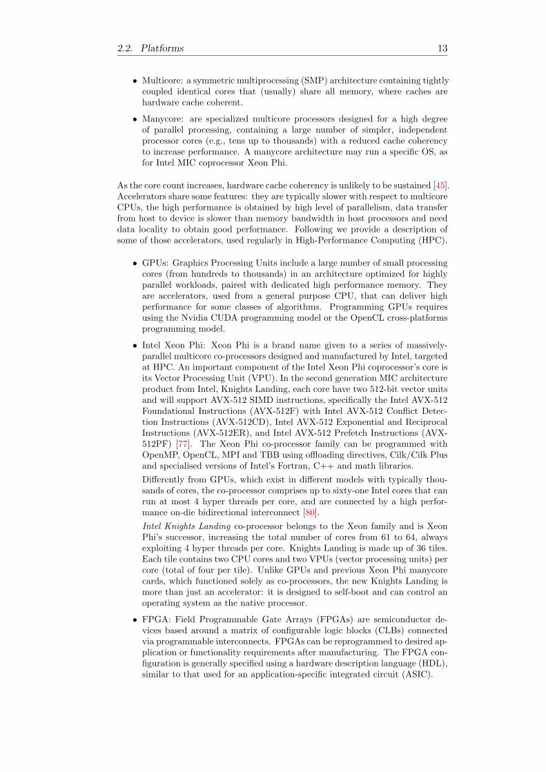
ProcessorProcessorProcessorProcessor
Main memory I/O system
One or
more levels
of cache
One or
more levels
of cache
One or
more levels
of cache
One or
more levels
of cache
Shared cache
Private
caches
Figure 2.1: Structure of an SMP.
data-level parallelism, but some overhead is introduced at least by thread commu-nication and synchronization. This overhead means the grain size (i.e., the ratio ofcomputation to the amount of communication), which is a key factor for efficientexploitation of thread-level parallelism.
The most common MIMD computers are multiprocessors, defined as computersconsisting of tightly coupled processors that share memory through a shared addressspace. Single-chip systems with multiple cores are known as multicores. Symmetric(shared-memory) multiprocessors (SMPs) typically feature small numbers of cores(nowadays from 12 to 24), where processors can share a single centralized memory,to which they all have equal access to (Fig. 2.1). In multicore chips, the memoryis effectively centralized, and all existing multicores are SMPs. SMP architecturesare also sometimes called uniform memory access (UMA) multiprocessors, arisingfrom the fact that all processors have a uniform latency from memory, even if thememory is organized into multiple banks.
The alternative design approach consists of multiprocessors with physically dis-tributed memory, called Distributed-Memory Systems (DSM). To support largernumbers of processors, memory must be distributed rather than centralized; oth-erwise, the memory system would not be able to support the bandwidth demandsof processors without incurring excessively long access latency. Such architecturesare known as nonuniform memory access (NUMA), since the access time dependson the location of a data word in memory.
Memory consistency model
The memory model, or memory consistency model, specifies the values that a sharedvariable read in a multithreaded program is allowed to return. The memory modelaffects programmability, performance and portability by constraining the transfor-mations that any part of the system may perform. Moreover, any part of the system(hardware or software) that transforms the program must specify a memory model,and the models at the different system levels must be compatible [[37, 115]]. Themost basic model is the Sequential Consistency, in which all instructions executedby threads in a multithreaded program appear in a total order that is consistent withthe program order on each thread [88]. Some programming languages offer sequen-tially consistency in a multiprocessor environment: in C++11, all shared variablescan be declared as atomic types with default memory ordering constraints. In Java,all shared variables can be marked as volatile.

12 Chapter 2. Technical Background
For performance gains, modern CPUs often execute instructions out of order tofully utilize resources. Since the hardware enforces instructions integrity, it canbe noticed in a single thread execution. However, in a multithreaded execution,reordering may lead to unpredictable behaviors.
Different CPU families have different memory models, thus different rules concern-ing memory ordering, but also the compiler optimizes the code by reordering in-structions. To guarantee Sequential Consistency, you must consider how to preventmemory reordering. Ways can be lightweight synchronizations or fences, full fence,or acquire/release semantics. Sequential Consistency restricts many common com-piler and hardware optimizations and to overcome the performance limitations ofthis memory model, hardware vendors and researchers have proposed several relaxedmemory models reported in [4].
In lock-free programming for multicore (or any symmetric multiprocessor), sequen-tial consistency must be ensured by preventing memory reordering. Herlihy andShavit [74] provide the following definition of lock-free programs: ”In an infiniteexecution, infinitely often some method call finishes”. In other words, as long asthe program is able to keep calling lock-free operations, the number of completedcalls keeps increasing. It is algorithmically impossible for the system to lock up dur-ing those operations. C/C++ and Java provide portable ways of writing lock-freeprograms with sequential consistency or even weaker consistency models.
For such purpose of writing sequentially consistent multithreaded programs, C++introduced the atomics standard library, which provides fine-grained atomic opera-tions [37] that guarantee Sequential Consistency only for data race free programs,hence allowing also lockless concurrent programming. Each atomic operation is in-divisible with regards to any other atomic operation that involves the same object.Atomic objects are free of data races.
Cache coherence and false sharing
SMP machines usually support the caching of both shared and private data, reduc-ing the average access time as well as the required memory bandwidth. Unfortu-nately, caching shared data introduces a new problem because the view of memoryheld by two different processors is through their individual caches, which could endup seeing two different values. This problem is generally referred to as the cachecoherence problem and several protocols have been designed to guarantee cache co-herence. In cache-coherent SMP machines, false sharing is a subtle source of cachemiss, which arises from the use of an invalidation-based coherence algorithm. Falsesharing occurs when a block is invalidated (and a subsequent reference causes amiss) because some word in the block, other than the one being read, is writteninto. In a false sharing miss, the block is shared, but no word in the cache is actuallyshared, and the miss would not occur if the block size were a single word.
2.2.2 Manycore processors
Manycore processors are specialized multi-core processors designed to exploit a highdegree of parallelism, containing a large number of simpler, independent processorcores, often called Hardware accelerators. A manycore processor contains at leasttens of cores and usually distributed memory, which are connected (but physicallyseparated) by an interconnect that has a communication latency of multiple clockcycles [110]. A multicore architecture equipped with hardware accelerators is a formof heterogeneous architecture. Comparing multicore to manycore processors, we cancharacterize them as follows:
2.2. Platforms 13
• Multicore: a symmetric multiprocessing (SMP) architecture containing tightlycoupled identical cores that (usually) share all memory, where caches arehardware cache coherent.
• Manycore: are specialized multicore processors designed for a high degreeof parallel processing, containing a large number of simpler, independentprocessor cores (e.g., tens up to thousands) with a reduced cache coherencyto increase performance. A manycore architecture may run a specific OS, asfor Intel MIC coprocessor Xeon Phi.
As the core count increases, hardware cache coherency is unlikely to be sustained [45].Accelerators share some features: they are typically slower with respect to multicoreCPUs, the high performance is obtained by high level of parallelism, data transferfrom host to device is slower than memory bandwidth in host processors and needdata locality to obtain good performance. Following we provide a description ofsome of those accelerators, used regularly in High-Performance Computing (HPC).
• GPUs: Graphics Processing Units include a large number of small processingcores (from hundreds to thousands) in an architecture optimized for highlyparallel workloads, paired with dedicated high performance memory. Theyare accelerators, used from a general purpose CPU, that can deliver highperformance for some classes of algorithms. Programming GPUs requiresusing the Nvidia CUDA programming model or the OpenCL cross-platformsprogramming model.
• Intel Xeon Phi: Xeon Phi is a brand name given to a series of massively-parallel multicore co-processors designed and manufactured by Intel, targetedat HPC. An important component of the Intel Xeon Phi coprocessor’s core isits Vector Processing Unit (VPU). In the second generation MIC architectureproduct from Intel, Knights Landing, each core have two 512-bit vector unitsand will support AVX-512 SIMD instructions, specifically the Intel AVX-512Foundational Instructions (AVX-512F) with Intel AVX-512 Conflict Detec-tion Instructions (AVX-512CD), Intel AVX-512 Exponential and ReciprocalInstructions (AVX-512ER), and Intel AVX-512 Prefetch Instructions (AVX-512PF) [77]. The Xeon Phi co-processor family can be programmed withOpenMP, OpenCL, MPI and TBB using offloading directives, Cilk/Cilk Plusand specialised versions of Intel’s Fortran, C++ and math libraries.
Differently from GPUs, which exist in different models with typically thou-sands of cores, the co-processor comprises up to sixty-one Intel cores that canrun at most 4 hyper threads per core, and are connected by a high perfor-mance on-die bidirectional interconnect [80].
Intel Knights Landing co-processor belongs to the Xeon family and is XeonPhi’s successor, increasing the total number of cores from 61 to 64, alwaysexploiting 4 hyper threads per core. Knights Landing is made up of 36 tiles.Each tile contains two CPU cores and two VPUs (vector processing units) percore (total of four per tile). Unlike GPUs and previous Xeon Phi manycorecards, which functioned solely as co-processors, the new Knights Landing ismore than just an accelerator: it is designed to self-boot and can control anoperating system as the native processor.
• FPGA: Field Programmable Gate Arrays (FPGAs) are semiconductor de-vices based around a matrix of configurable logic blocks (CLBs) connectedvia programmable interconnects. FPGAs can be reprogrammed to desired ap-plication or functionality requirements after manufacturing. The FPGA con-figuration is generally specified using a hardware description language (HDL),similar to that used for an application-specific integrated circuit (ASIC).
14 Chapter 2. Technical Background
2.2.3 Distributed Systems, Clusters and Clouds
A distributed system is a model in which components located on networked com-puters communicate and coordinate their actions by passing messages. It can becomposed by various hardware and software components, thus exploiting homoge-neous and heterogeneous architectures. An important aspect of distributed com-puting architectures is the method of communicating and coordinating work amongconcurrent processes. Through various message passing protocols, processes maycommunicate directly with one another, typically in a master-slave relationship,operating to fulfill the same objective. This master-slave relationship reflects thetypical execution model of Big Data analytics tools on distributed systems: the mas-ter process is assigned to coordinate slaves execution (typically called workers) andcoordination. Slaves may execute the same program or part of the computation, andthey communicate with each other and with the master by message passing. Mas-ter and slaves may also exchange data via serialization. From the implementationviewpoint, those architectures are typically programmed by exploiting the MessagePassing Interface (MPI) [105], a language-independent communication protocol usedfor programming parallel computers, as well as a message-passing API that supportspoint-to-point and collective communication by means of directly callable routines.Many general-purpose programming languages have bindings to MPI’s functional-ities, among which: C, C++, Fortran, Java and Python. Moving to the Big Dataworld, tools are often implemented in Java in order to easily exploit facilities such asJava RMI API [103], which performs remote method invocation supporting directtransfer of serialized Java classes and distributed garbage collection. These modelsfor communication will be further investigated in Section 2.3.3.
In contrast with shared-memory architectures, clusters look like individual comput-ers connected by a network. Since each processor has its own address space, thememory of one processor cannot be accessed by another processor without the as-sistance of software protocols running on both processors. In such design, message-passing protocols are used to communicate data among processors. Clusters areexamples of loosely coupled MIMDs. These large-scale systems are typically usedfor cloud computing with a model that assumes either massive numbers of indepen-dent requests or highly parallel intensive compute tasks.
There are two classes of large-scale distributed systems:
1) Private clouds, in particular multicore clusters, which are inter networked —possibly heterogeneous — multicore devices.
2) Public clouds, which are (physical or virtual) infrastructures offered by providersin the form of inter networked clusters. In the most basic public cloud model,providers of IaaS (Infrastructures-as-a-Service) offer computers — physical or (moreoften) virtual machines — and other resources on-demand. Public IaaS clouds canbe regarded as virtual multicore clusters. The public cloud model encompasses apay-per-use business model. End users are not required to take care of hardware,power consumption, reliability, robustness, security, and the problems related tothe deployment of a physical computing infrastructure.
2.3 Parallel Programming Models
Shifting from sequential to parallel computing, a trend largely motivated by theadvent of multicore platforms, does not always translate into greater CPU perfor-mance: multicores are small-scale but full-fledged parallel machines and they retainmany of their usage problems. In particular, sequential code will get no performancebenefits from them: a workstation equipped with a quad-core CPU but running se-quential code is wasting 3
4 of its computational power. Developers are then facing

2.3. Parallel Programming Models 15
the challenge of achieving a trade-off between performance and human productivity(total cost and time to solution) in developing and porting applications to multicoreand parallel platforms in general.
Therefore, effective parallel programming happens to be a key factor for efficientparallel computing, but efficiency is not the only issue faced by parallel program-mers: writing parallel code that is portable on different platforms and maintainableare tasks that programming models should address.
2.3.1 Types of parallelism
Types of parallelisms can be categorized in four main classes:
• Task Parallelism consists of running the same or different code (task) ondifferent executors (cores, processors, etc.). Tasks are concretely performedby threads or processes, which may communicate with one another as theyexecute. Communication takes place usually to pass data from one thread tothe next as part of a graph. Task parallelism does not necessarily concernstream parallelism, but there might cases in which the computation of eachsingle item in a input stream embeds an independent (thus parallel) task, thatcan efficiently be exploited to speedup the application. The farm pattern isa typical representation of such class of patterns, as we will describe in nextsections.
• Data Parallelism is a method for parallelizing a single task by processingindependent data elements in parallel. The flexibility of the technique re-lies upon stateless processing routines implying that the data elements mustbe fully independent. Data Parallelism also supports Loop-level Parallelismwhere successive iterations of a loop working on independent or read-onlydata are parallelized in different flows-of-control (according to the model co-begin/co-end) and concurrently executed.
• Stream Parallelism is a method for parallelizing the execution (aka. filtering)of a stream of tasks by segmenting each task into a series of sequential1 orparallel stages. This method can be also applied when there exists a totalor partial order, respectively, in a computation preventing the use of dataor task parallelism. This might also come from the successive availability ofinput data along time (e.g., data flowing from a device). By processing dataelements in order, local state may be either maintained in each stage or dis-tributed (replicated, scattered, etc.) along streams. Parallelism is achievedby running each stage simultaneously on subsequent or independent data el-ements.
• DataFlow Parallelism is a programming paradigm modeling a (parallel) pro-gram as a directed graph where operations are represented by nodes, andedges model data dependencies. Nodes in this graph represent functionalunit of computation over data item (tokens) flowing on edges. In contrastwith procedural (imperative) programming model, a DataFlow program isdescribed as a set of operations and connections among them, defined as aset of input and output edges. Operations execute as soon as all their inputedges have an incoming token available and operations without a direct de-pendence can be run in parallel. This model, formalized by Kahn [83], is oneof the main building blocks of the model proposed in this thesis. A furtherdescription is provided in subsequent sections.
Since Data Parallelism and Dataflow Parallelism are important aspects in this work,we explore them further in the next two paragraphs.
1In the case of total sequential stages, the method is also known as Pipeline Parallelism.

16 Chapter 2. Technical Background
f(x )i
f(x )i
f(x )i
f(x )i1x
2x
n-1xn-2xn-3x
0x
1y
2y
n-1yn-2yn-3y
0y
Figure 2.2: A general representation of a Map data parallelpattern. Input data structure is partitioned according tothe number of workers. Business logic function is replicated
among each worker.
Data parallelism
A data-parallel computation performs the same operation on different items of agiven data structure at the same time. Opposite to task parallelism, which empha-sizes the parallel nature of the computation, data parallelism stresses the parallelnature of the data2.
Formally, a data parallel computation is characterized by partitioning data struc-tures and function replication: a common partitioning approach divides input databetween the available processors. Depending on the algorithm, there might be casesin which data dependencies exist among partitioned subtasks: many data-parallelprograms may suffer from bad performance and poor scalability because of a highnumber of data dependencies or a low amount of inherent parallelism.
Here we present two widely used instances of data parallel patterns, namely themap and the reduce patterns, that are also the most often used patterns in BigData scenarios. Other data parallel patterns exist, which basically permit to applyhigher-order functions to all the elements of a data structure. Among them wecan mention the fold pattern and the scan (or prefix sum) pattern. There is alsothe stencil pattern, which is a generalization of the map pattern, and under afunctional perspective both patterns are similar, but the stencil encompasses allthose situations that require data exchange among workers [12].
Map
The map pattern is a straightforward case of data parallel paradigm: given a func-tion f that expresses an application’s behavior, and a data collection X of knownsize (e.g., a vector with n elements), a map pattern will apply the function f to allthe elements xi ∈ X:
yi = f(xi) ∀i = 0, . . . , n− 1 .
Each element yi of the resulting output vector Y is the result of a parallel compu-tation. A pictorial representation of the map pattern is presented in Fig. 2.2.
Notable examples that naturally fit this paradigm include some vector operations(scalar-vector multiplication, vector sum, etc.), matrix-matrix multiplication (in
2We denote this difference by using a zero-based numbering when indexing data struc-tures in data parallel patterns.

2.3. Parallel Programming Models 17
1x2xn-1x n-2x n-3x 0x
Figure 2.3: A general Reduce pattern: the reduction isperformed in parallel organizing workers in a tree-like struc-ture: each worker computes the function ⊕ on the resultscommunicated by the son worker. The root worker delivers
the reduce result.
which the result matrix is partitioned, the input matrices replicated), the Mandel-brot set calculation, and many others.
Reduce
A reduce pattern applies an associative binary function (⊕) to all the elements ofa data structure. Given a vector X of length n, the reduce pattern computes thefollowing result:
x0 ⊕ x1 ⊕ . . .⊕ xn−1 .
In Figure 2.3, we report an example of a possible implementation of a reduce pattern,in which the reduce operator is applied over the assigned partition of the vector inparallel, and each single result is then used to compute a global reduce. In a tree-like organization, leaf nodes compute their local reduce and then propagate resultsto parent nodes; the root node delivers the reduce result.
While the reduce pattern is straightforward for associative and commutative oper-ators (e.g., addition and multiplication of real numbers is associative), this is nomore true for floating point operators. Floating-point operations, as defined in theIEEE-754 standard, are not associative [1]. Studies demonstrated how, on massivelymulti-threaded systems, the non-deterministic nature of how machine floating-pointoperations are interleaved, combined with the fact that intermediate values have tobe rounded or truncated to fit in the available precision leads to non-deterministicnumerical error propagation [129].
The composition of a map step and a reduce step generates the Map+Reduce pat-tern, in which a function is first applied, in parallel, to all elements of a datastructure, and then the results from the map phase are merged using some reduc-tion function (see Figure 2.4). This is an important example of the composabilityallowed by parallel patterns, which permits to define a whole class of algorithms fordata-parallel computation.
The functional composition of these two parallel patterns is the basis of Google’sMapReduce distributed programming model and framework [61], which exploits key-value pairs to compute problems that can be parallelized by mapping a function

18 Chapter 2. Technical Background
Figure 2.4: A Map+Reduce pattern.
over a given dataset and then combining the results. Likely, it is the largest pat-tern framework in use, and spun off different open-source implementations, such asHadoop [130] and Phoenix [109].
Both Map and Reduce patterns are exploited in PiCo and they are further describedin Chapter 5.
2.3.2 The Dataflow Model
Dataflow Process Networks are a special case of Kahn Process Networks, a modelof computation that describes a program as a set of concurrent processes commu-nicating with each other via FIFO channels, where reads are blocking and writesare non-blocking [83]. In a Dataflow process network, a set of firing rules is associ-ated with each process, called actor. Processing then consists of “repeated firingsof actors”, where an actor represents a functional unit of computation over tokens.For an actor, to be functional means that firings have no side effects—thus actorsare stateless—and the output tokens are pure functions of the input tokens. Themodel can also be extended to allow stateful actors.
A Dataflow network can be executed mainly by two classes of execution, namelyprocess-based and scheduling-based—other models are flavors of these two. Theprocess-based model is straightforward: each actor is represented by a process thatcommunicates via FIFO channels. In the scheduling-based model—also known asdynamic scheduling—a scheduler tracks the availability of tokens in input to actorsand schedules enabled actors for execution; the atomic unit being scheduled isreferred as a task and represents the computation performed by an actor over asingle set of input tokens.
Actors
A Dataflow actor consumes input tokens when it fires and then produces outputtokens; thus it repeatedly fires on tokens arriving from one or more streams. The
2.3. Parallel Programming Models 19
function mapping input to output tokens is called the kernel of an actor.3 A firingrule defines when an actor can fire. Each rule defines what tokens have to beavailable for the actor to fire. Multiple rules can be combined to program arbitrarilycomplex firing logics (e.g., the If node).
Input channels
The kernel function takes as input one or more tokens from one or more inputchannels when a firing rule is activated. The basic model can be extended to allowfor testing input channels for emptiness, to express arbitrary stream consumingpolicies (e.g., gathering from any channel).
Output channels
The kernel function places one or more tokens into one or more output channelswhen a firing rule is activated. Each output token produced by a firing can bereplicated and placed onto each output channel (i.e., broadcasting) or sent to specificchannels, in order to model arbitrarily producing policies (e.g., switch, scatter).
Stateful actors
Actors with state can be considered like objects (instead of functions) with methodsused to modify the object’s internal state. Stateful actors is an extension that allowsside effects over local (i.e., internal to each actor) states. It was shown by Lee andParks [91] that stateful actors can be emulated in the stateless Dataflow modelby adding an extra feedback channel carrying the value of the state to the nextexecution of the kernel function on the next element of the stream and by definingappropriate firing rules.
In the next sections, we provide a description of various other low-level and high-level programming models and techniques.
2.3.3 Low-level approaches
Typically, low-level approaches provide the programmers only with primitives forflow-of-control management (creation, destruction), their synchronization and datasharing, which are usually accomplished in critical regions accessed in mutual exclu-sion (mutex). As an example, POSIX thread library can be used for this purpose.Parallel programming languages are usually extensions to well-established sequen-tial languages, such as C/C++, Java or Fortran, where the coordination of multipleexecution flows is either obtained by means of external libraries, linked at compiletime to the application source code (e.g., Pthreads, OpenMP, MPI ), or enrichedwith specific constructs useful to orchestrate the parallel computation, for instanceconsider the Java Concurrency API and the C++11 standard published in 2011,which introduced multithreaded programming. The well known report, authoredby H. Boehm [36], provides specific arguments that a pure library approach, inwhich the compiler is designed independently of threading issues, cannot guaranteecorrectness of the resulting code. It is illustrated that there are very simple cases(concurrent modification, adjacent data rewriting and register promotion) in which
3The Dataflow Process Network model also seamlessly comprehends the MacroDataflow parallel execution model, in which each process executes arbitrary code. Con-versely, an actor’s code in a classical Dataflow architecture model is typically a singlemachine instruction. In the following, we consider Dataflow and Macro Dataflow to beequivalent models.

20 Chapter 2. Technical Background
a pure library-based approach seems incapable of expressing an efficient parallelalgorithm.
Programming parallel complex applications in this way is certainly hard; tuningthem for performance is often even harder due to the non-trivial effects induced bymemory fences (used to implement mutex) on data replicated in core’s caches.
Indeed, memory fences are one of the key sources of performance degradation incommunication intensive (e.g., streaming) parallel applications. Avoiding memoryfences means not only avoiding locks but also any kind of atomic operation inmemory (e.g., Compare-And-Swap, Fetch-and-Add). While there exists severalassessed fence-free solutions for asynchronous symmetric communications,4 theseresults cannot be easily extended to asynchronous asymmetric communications5,which are necessary to support arbitrary streaming networks. This ability is one ofthe core features of FastFlow (2.4.1).
A first way to ease the programmer’s task and improve program efficiency consistsin raising the level of abstraction of concurrency management primitives. As anexample, threads might be abstracted out in higher-level entities that can be pooledand scheduled in user space possibly according to specific strategies to minimizecache flushing or maximize load balancing of cores. Synchronization primitives canbe also abstracted out and associated to semantically meaningful points of the code,such as function calls and returns, loops, etc. Intel Threading Building Block (TBB)[78], OpenMP [106], and Cilk [47] all provide this kind of abstraction — each ofthem in its own way. This kind of abstraction significantly simplifies the hand-coding of applications but it is still too low-level to effectively (semi-)automatizethe optimization of the parallel code. In the following paragraphs, we describe abit more in detail a list of low level parallel programming frameworks and APIs.
POSIX Threads (or Pthreads) [40] are one of the most famous low-level paral-lel programming APIs for shared-memory environments, defined by the standardPOSIX.1c, Threads extensions (IEEE Std 1003.1c-1995). They are present in ev-ery Unix-like operating system (Linux, Solaris, Mac OS X, etc.) and other POSIXsystems, giving access to OS-level threads and synchronization mechanisms. SincePthreads is a C library, it can be used in C++ programs as well, though therehave been much improvements in the C++11 standard aimed at facilitating shared-memory parallel programming from a low-level to a high-level parallel programming.We remark that ISO C++ is completely independent from POSIX and it is providedalso in non-POSIX platforms.
Message Passing Interface (MPI) [105] is a language-independent communica-tion protocol used for programming parallel computers, as well as a message-passingAPI that supports point-to-point and collective communication by means of directlycallable routines. Many general-purpose programming languages have bindings toMPI’s functionalities, among which: C, C++, Fortran, Java and Python.
Mainly targeted at distributed architectures, MPI offers specific implementations foralmost any high-performance interconnection network. At the same time, shared-memory implementations exist, that allow the use of MPI even on NUMA andmulti-processors systems.
MPI allows to manage synchronization and communication functionalities amonga set of processes, and provides mechanisms to deploy a virtual topology of thesystem upon which the program is executing. These features, supported by a richset of capabilities and functions, clearly require high programming and networkingskills: MPI has long been the lingua franca of HPC, supporting the majority ofall supercomputing work scientists and engineers have relied upon for the past twodecades. Nonetheless, MPI is at a low level of abstraction for application writers:
4Single-Producer-Single-Consumer (SPSC) queues [89].5Multiple-Producer-Multiple-Consumer queues (MPMC).

2.3. Parallel Programming Models 21
using MPI means programming at the transport layer, where every exchange ofdata has to be implemented through sends and receives, data structures must bemanually decomposed across processors and every update of the data structureneeds to be recast into a flurry of messages, synchronizations, and data exchange.
OpenMP [106] is considered by many the de facto standard API for shared-memoryparallel programming. OpenMP is an extension that can be supported by C, C++and Fortran compilers and defines an “accelerator-style” programming, where themain program is run sequentially while code is accelerated in specific points, runningin parallel, using special preprocessor instructions known as pragmas. Compilersthat do not support specific pragmas can ignore them, making an OpenMP programcompilable and runnable on every system with a generic sequential compiler.
While Pthreads are low-level and require the programmer to specify every detailof the behavior of each thread, OpenMP allows to simply state which block ofcode should be executed in parallel, leaving to compiler and run-time system theresponsibility to determine the details of the thread behavior. This feature makesOpenMP programs simpler to code, with a risk of unpredictable performance thatstrongly depends on compiler implementations and optimizations. For instance,in [111] OpenMP limitations have been demonstrated such as its inability to performreductions on complex data types as well as scheduling issues on applications withirregular computations (such as the Mandelbrot benchmark).
OpenCL [85] is an API designed to write parallel programs that execute acrossheterogeneous architectures, and allows the users to exploit GPUs for general pur-pose tasks that can be parallelized. It is implemented by different hardware ven-dors such as Intel, AMD and NVIDIA, making it highly portable and allowingOpenCL code to be run on different hardware accelerators. OpenCL allows the im-plementation of applications onto FPGAs, allowing software programmers to writehardware-accelerated kernel functions in OpenCL C, an ANSI C-based languagewith additional OpenCL constructs. OpenCL represents an extension to C/C++but must be considered a low-level language, focusing on low-level features manage-ment rather than high-level parallelism exploitation patterns. It has the capabilityto revert to the CPU for execution when there is no GPU in the system, and itsportability makes it suitable for hybrid (CPU/GPU) or cloud based environments.
Java provides multi-threading and RPC support (Java RMI API) that can beused to write parallel applications for both shared memory and distributed memoryarchitectures [103]. The original implementation depends on Java Virtual Machine(JVM) class representation mechanisms and it only supports making calls from oneJVM to another. However, while being a high-level sequential language, parallelsupport is provided in a low-level fashion, possibly lower than OpenMP.
2.3.4 High-level approaches
Parallel programming has always been related to HPC environments, where pro-grammers write parallel code by mean of low-level libraries that give complete con-trol over the parallel application, allowing them to manually optimize the code inorder to exploit at best the parallel architecture. This programming methodol-ogy has become unsuitable with the fast move to heterogeneous architectures, thatencompass hardware accelerators, distributed shared-memory systems and cloudinfrastructures, highlighting the need for proper tools to easily implement parallelapplications.
It is widely acknowledged that the main problem to be addressed by a parallelprogramming model is portability : the ability to not only compile and execute thesame code on different architectures and obtain the same top performance [58], butalso — and even more complex — the challenge of performance portability, thatis, implementing applications that scale on different architectures. A high-level

22 Chapter 2. Technical Background
approach to parallel programming is a better way to go if we want to address thisproblem, so that programmers can build parallel applications and be sure that theywill perform reasonably well on the wide choice of parallel architectures availabletoday [114].
Attempts to raise the level of abstraction and reduce the programming effort dateback to at least three decades. Notable results have been achieved by the algo-rithmic skeleton approach [48] (aka. pattern-based parallel programming), that hasgained popularity after being revamped by several successful parallel programmingframeworks. Despite some criticisms — mostly related to the limited amount ofpatterns that might not be sufficient to allow a decent parallelization of most al-gorithms — algorithmic skeletons success has been determined by the numerousadvantages it has compared to traditional parallel programming frameworks.
2.3.5 Skeleton-based approaches
Algorithmic skeletons have been initially proposed by Cole [49] to provide prede-fined parallel computation and communication patterns, hiding parallelism manage-ment from the user. Algorithmic skeletons capture common parallel programmingparadigms (e.g., Map+Reduce, ForAll, Divide&Conquer, etc.) and make themavailable to the programmer as high-level programming constructs equipped withwell-defined functional and extra-functional semantics [11]. Ideally, algorithmicskeletons address the difficulties of parallel programming (i.e., concurrency exploita-tion, orchestration, mapping, tuning) moving them from the application design todevelopment tools, by capturing and abstracting common paradigms of parallelprogramming and providing them with efficient implementations. This idea can beconsidered at the core of structured parallel programming : expressing the parallelcode as a composition of simple “building blocks”.
Literature review of skeleton-based approaches
Many skeletons have been proposed in literature in the last two decades coveringmany different usage schema of the three classes of parallelism, on top of both themessage passing [50, 57, 113, 9, 16, 35, 108, 13, 61, 10] and shared memory [7, 78]programming models.
Here, we discuss some skeleton libraries that target C/C++ as their execution lan-guage, and mostly focus on parallel programming for multi-core architectures. Fora broader survey of algorithmic skeletons, we refer to Gonzalez-Velez and Leyton’ssurvey [71].
P3L is one of the earliest proposal for pattern-based parallel programming [53]. P 3Lis a skeleton-based coordination language that manages the parallel or sequentialexecution of C code. It comes with a proper compiler for the language, and usesimplementation templates to compile the code into a target architecture. P 3Lprovides patterns for both stream parallelism and data parallelism.
SKELib [54] builds upon the contributions of P 3L by inheriting, among otherfeatures, the template system. It differs from P 3L because a coordination languageis no longer used, and skeletons are provided as a C library. It only offers stream-based skeletons (namely farm and pipe patterns).
SkeTo [95] is a C++ library based on MPI that provides skeletons for distributeddata structures, such as arrays, matrices, and trees. The current version is basedon C++ expression templates, used to represent part of an expression where thetemplate represents the operation and parameters represent the operands to whichthe operation applies.

2.3. Parallel Programming Models 23
SkePU [66] is an open-source skeleton programming framework for multi-coreCPUs and multi-GPU systems. It is a C++ template library with data-parallel andtask-parallel skeletons (map, reduce, map-reduce, farm) that also provides genericcontainer types and support for execution on multi-GPU systems, both with CUDAand OpenCL.
SkelCL [116] is a skeleton library targeting OpenCL. It allows the declaration ofskeleton-based applications hiding all the low-level details of OpenCL. The set ofskeletons is currently limited to data-parallel patterns: map, zip, reduce and scan,and it is unclear whether skeleton nesting is allowed. A limitation might come fromthe library’s target, which is restricted to the OpenCL language: it likely benefitsfrom the possibility to run OpenCL code both on multi-core and on many-corearchitectures, but the window for tunings and optimizations is thus quite restricted.
Muesli — Muenster Skeleton Library [46] — is a C++ template library that sup-ports shared-memory multi-processor and distributed architectures using MPI andOpenMP as underlying parallel engines. It provides data parallel patterns such asmap, fold (i.e., reduce), scan (i.e., prefix sum), and distributed data structures likedistributed arrays, matrices and sparse matrices. Skeleton functions are passed todistributed objects as pointers, since each distributed object has skeleton functionsas internal member of the class itself. The programmer must explicitly indicatewhether GPUs are to be used for data parallel skeletons, if available.
Intel Threading Building Blocks (TBB) [78] defines a set of high-level paral-lel patterns that permit to exploit parallelism independently from the underlyingplatform details and threading mechanisms. It targets shared-memory multi-corearchitectures, and exposes parallel patterns for exploiting both stream parallelismand data parallelism. Among them, the parallel for and parallel foreach
methods may be used to parallelize independent invocation of the function bodyof a for loop, whose number of iterations is known in advance. C++11 lambdaexpression can be used as arguments to these calls, so that the loop body functioncan be described as part of the call, rather than being separately declared. Theparallel for uses a divide-and-conquer approach, where a range [0, num iter) issplitted into sub-ranges and each sub-range r can be processed as a separate taskusing a serial for loop.
GrPPI [62] is a generic high-level pattern interface for stream-based C++ appli-cations. Thanks to its high-level C++ API, this interface allows users to easilyexpose parallelism in sequential applications using already existing parallel frame-works, such as C++ threads, OpenMP and Intel TBB. It is implemented using C++template meta-programming techniques to provide interfaces of a generic, reusableset of parallel patter patterns without incurring in runtime overheads. GrPPI tar-gets the following stream parallel processing patterns: Pipeline, Farm, Filter andStream-Reduce. Parallel versions and to implement the proposed interfaces are im-plemented by we leveraging C++11 threads and OpenMP, and the pattern-basedparallel framework Intel TBB. These patterns are parametrized by user definedlambdas and they are nestable.
FastFlow [15] is a parallel programming framework originally designed to supportstreaming applications on cache-coherent multicore platforms. It will be describedmore in detail in Section 2.4.1, since it is part of the PiCo runtime.
2.3.6 Skeletons for stream parallelism
A stream-parallel program can be naturally represented as a graph of independentstages (kernels or filters) which communicate over data channels. Conceptually, astreaming computation represents a sequence of transformations on the data streams

24 Chapter 2. Technical Background
in the program. Parallelism is achieved by running each stage of the graph simul-taneously on subsequent or independent data elements. Several skeletons exist thatsupport stream-parallel programming.
The Pipeline skeleton is one of the most widely-known pattern (see Fig. 2.5). Par-allelism is achieved by running each stage simultaneously on subsequent data ele-ments, with the pipeline’s throughput being limited by the throughput of the sloweststage. It is typically used to model computations expressed in stages, and in thegeneral case a pipeline has at least two stages. Given a sequence x1, . . . , xk of inputtasks and the simplest form of a pipeline with three stages, the computation oneach single task xi is expressed as the composition of three functions f , z and g,where the second stage (function z) executes on the results of the application ofthe first stage, z(f(xi)), and third stage applies the function z on the output of thesecond stage: g(z(f(xi))).
r1xk-1 p = rk rk-1p = f(x )ii r = g(q )i ix1xk p = q = z(p ) ii
Figure 2.5: A general Pipeline pattern with three stages.
The parallelization is obtained by concurrently executing all the stages onto differentconsecutive items of the input stream. In the general form, a pipeline with stagess1, . . . , sm computes the output stream
sm(sm−1(. . . s2(s1(xk)) . . .)), . . . , sm(sm−1(. . . s2(s1(x1)) . . .)) .
The sequential code has to be described in terms of function composition, where theoutput of each stage is sent to the next one, respecting the function ordering. Thesemantic of the pipeline paradigm ensures that all stages will execute in parallel.
The Farm skeleton models functional replication and consists in running multipleindependent stages in parallel, each operating on different tasks of the input stream,thus it is often used to model embarrassingly parallel computations.
The Farm skeleton can be better understood as a three stage — emitter, workers,collector — pipeline (see Fig. 2.6). The emitter dispatches stream items to a set ofworkers, which independently elaborate different items. The output of the workersis then gathered by the collector into a single stream. More complex combinationsof both patterns are possible, such as a pipeline of farms, where each stage of thepipeline is, in fact, a farm (as in Figure 2.7).
x1 y1xk-1 yk yk-1emitter collectorxk
f(x )i
f(x )i
f(x )i
f(x )i
s1 s3
s2
Figure 2.6: A simple Farm pattern with an optional col-lector stage, whose stroke is dashed. Background light-grayboxes show that a farm pattern can be embedded into a
three-stages pipeline.

2.4. Programming multicore clusters 25
x1 y1xk-1 yk yk-1xk E C
W
W
W
W
s1
1 1
1
1
1
11
E C
W
W
W
W
s2
2 2
2
2
2
2
Figure 2.7: A combination of pipeline and farm patterns,where each stage of a two-stage pipeline is a farm. In this fig-ure, subscripts in farms components are used to distinguish
the two farms.
The Loop skeleton (also known as feedback), provides a way to generate cycles in astream graph. By using a feedback channel, it is possible to route back results inorder to implement iterative computations. This skeleton is typically used togetherwith the farm skeleton to model recursive and Divide&Conquer computations, inwhich an input task is recursively sub-divided in sub-tasks until a condition is met,then each sub-task is executed and results are merged. For instance, in a Farmpattern as in Fig. 2.6 we can connect the Collector to the Emitter with a feedbackchannel. In general it is possible to connect Farm, Pipeline and feedback channelsto build more complex networks.
2.4 Programming multicore clusters
Programming tools and frameworks are needed to efficiently target architectureshosting inter networked — possibly heterogeneous — multicore devices, which ap-pear to be the reference architecture ferrying programmers from the mainly sequen-tial to mainly parallel programming era [29].
Shared-memory multicores and clusters/networks of processing elements requirequite different techniques and tools to support efficient parallelism exploitation.The de facto standard tools in both cases are OpenMP [106] and MPI [105], usedeither alone or in conjunction. Despite being efficient on some classes of applications,OpenMP and MPI share a common set of problems: poor separation of concernsamong application and system aspects, a rather low level of abstraction presented tothe application programmers, and poor support for really fine grained applications.
At the moment, it is not clear if the mixed MPI/OpenMP programming modelalways offers the most effective mechanisms for programming clusters of SMP sys-tems [41]. Furthermore, when directly using communication libraries such as MPI,the abstraction level is rather low and the programmer has to think about decompos-ing the problem, integrating the partial solutions, and bother with communicationproblems such as deadlocks and starvation.
Therefore, we advocate the use of high-level parallel programming frameworks tar-geting hybrid multicore and distributed platforms as a vehicle for building efficientparallel software — possibly derived semi-automatically from sequential code —featuring performance portability over heterogeneous parallel platforms.
2.4.1 FastFlow
FastFlow [56] is an open source, structured parallel programming framework sup-porting highly efficient stream parallel computation while targeting shared memorymulticores. Its efficiency mainly comes from the optimized implementation of thebase communication mechanisms and from its layered design. It provides a set of

26 Chapter 2. Technical Background
ready-to-use, parametric algorithmic skeletons modeling the most common paral-lelism exploitation patterns, which may be freely nested to model more complexparallelism exploitation patterns. It is realized as a C++ pattern-based parallelprogramming framework aimed at simplifying the development of applications for(shared-memory) multi-core and GPGPU platforms.
The key vision of FastFlow is that ease-of-development and runtime efficiency canboth be achieved by raising the abstraction level of the design phase. FastFlowprovides a set of algorithmic skeletons addressing both stream parallelism — withthe farm and pipeline patterns — and data parallelism — providing stencil, map,reduce pattern, and their arbitrary nesting and composition [19]. Map, reduceand stencil patterns can be run both on multi-cores and offloaded onto GPUs. Inthe latter case, the user code can include GPU-specific statements (i.e., CUDA orOpenCL statements).
Leveraging the farm skeleton, FastFlow exposes a ParallelFor pattern [55], wherechunks of a loop iterations having the form for(idx=start;idx<stop;idx+=step)
are executed by the farm workers. Just like TBB, FastFlow’s ParallelFor patternuses C++11 lambda expression as a concise and elegant way to create functionobjects: lambdas can “capture” the state of non-local variables by value or byreference and allow functions to be syntactically defined when needed.
From the performance viewpoint, one distinguishing feature at the core of Fast-Flow is that it supports lock-free (fence-free) Multiple-Producer-Multiple-Consumer(MPMC) queues [18] that can support low-overhead high-bandwidth multi-partycommunications on multicore architectures, i.e., any streaming network, includingcyclic graphs of threads. The key intuition underneath FastFlow is to provide theprogrammer with lock-free MP queues and MC queues (that can be used in pipelineto build MPMC queues) to support fast streaming networks.
Traditionally, MPMC queues are built as passive entities: threads concurrentlysynchronize (according to some protocol) to access data; these synchronizations areusually supported by one or more atomic operations (e.g., Compare-And-Swap)that behave as memory fences. FastFlow design follows a different approach: toavoid any memory fence, the synchronizations among queue readers or writers arearbitrated by an active entity (e.g., a thread). We call these entities Emitter (E) orCollector (C) according to their role; they actually read an item from one or morelock-free SPSC queues and write onto one or more lock-free SPSC queues. Thisrequires a memory copy but no atomic operations.
The performance advantage of this solution comes from the higher speed of the copyoperation compared with the memory fence; this advantage is further increased byavoiding cache invalidation triggered by fences. This also depends on the size andthe memory layout of copied data. The former point is addressed using data pointersinstead of data, and ensuring that the data is not concurrently written: in manycases this can be derived by the semantics of the skeleton that has been implementedusing MPMC queues — as an example this is guaranteed in a stateless farm andmany other cases.
FastFlow design is layered (see Fig. 2.8). The lower layer, called simple streamingnetworks, basically provides two basic abstractions:
• process-component, i.e., a control flow realized with POSIX threads and pro-cesses, for multicore and distributed platforms respectively.
• 1-1 channel, i.e., a communication channel between two components, real-ized with wait-free single-producer/single-consumer queues (FF-SPSC) [14]or zero-copy ZeroMQ channels [134], for multicore and distributed platforms,respectively.

2.4. Programming multicore clusters 27
Core patternspipeline, farm, feedback
High-level patternsparallel_for, parallel_forReduce, …
Parallel applicationsefficient and portable
Multicore and many-core platformsClusters of multicore + many-core
FastFlow
CUDA TCP/IPIB/OFED
Building blocksqueues, ff_node, ...
OpenCL
Figure 2.8: Layered FastFlow design .
Both realizations of the 1-1 channel are top state-of-the-art in their classes, in termsof latency and bandwidth. As an example, FF-SPSC exhibits a latency down to 10nanoseconds per message on a standard Intel Xeon @2.0GHz [14].
1 class ff_node {
2 protected:
3 virtual bool push(void* data) { return qout->push(data); }
4 virtual bool pop(void** data) { return qin->pop(data); }
5 public:
6 virtual void* svc(void * task) = 0;
7 virtual int svc_init() { return 0; };
8 virtual void svc_end() {}
9 ...
10 private:
11 SPSC* qin;
12 SPSC* qout;
13 };
Listing 2.1: FastFlow ff node class schema.
Above this mechanism, the second layer — called arbitrary streaming networks —further generalizes the two concepts, providing:
• FastFlow node, i.e., the basic unit of parallelism that is typically identifiedwith a node in a streaming network. It is used to encapsulate sequentialportions of code implementing functions, as well as high-level parallel pat-terns such as pipelines and farms. From the implementation viewpoint, theff_node C++ class realizes a node in the shared-memory scenario and theff_dnode extends it in the distributed memory setting (see Listing 2.1).
• Collective channel, i.e., a collective communication channel, either amongff_nodes or many ff_dnodes.
Eventually, the third layer provides the farm, pipeline and other parallel patternsas C++ classes.
Each ff node is used to run a concurrent activity in a component, and it has twoassociated channels: one used to receive input data (pointers) to be processed andone to deliver the (pointers to the) computed results. Representing communicationand synchronization as a channel ensures that synchronisation is tied to communi-cation and allows layers of abstraction at higher levels to compose parallel programswhere synchronization is implicit. The svc method encapsulates the computation

28 Chapter 2. Technical Background
to be performed on each input datum to obtain the output result. svc_init andsvc_end methods are executed when the application is started and before it is ter-minated. The three methods should be provided by the programmer in order toinstantiate an ff node.
Distributed FastFlow
FastFlow also provides an implementation running on distributed systems, basedon the ZeroMQ library. Briefly, ZeroMQ is an LGPL open-source communicationlibrary [134] providing the user with a socket layer that carries whole messagesacross various transports: inter-thread communications, inter-process communica-tions, TCP/IP, and multicast sockets. ZeroMQ offers an asynchronous communica-tion model, which provides a quick construction of complex asynchronous message-passing networks, with reasonable performance.
A ff dnode (distributed ff node) provides an external channel specialized toprovide different patterns of communication. The set of communication collectivesallows one to provide exchange of messages among a set of distributed nodes, usingwell-known predefined patterns. The semantics of each communication patterncurrently implemented are summarized in Table 2.1. In the current version (seeFig. 2.8), which supports distributed platforms, many graphs of ff nodes can beconnected by way of ff dnodes (which support network collective channels), thusproviding a useful abstraction for effective programming of hybrid multicore anddistributed platforms.
Pattern Description
unicast unidirectional point-to-point communication betweentwo peers
broadcast sends the same input data to all connected peers
scatter sends different parts of the input data, typically par-titions, to all connected peers
onDemand the input data is sent to one of the connected peers,the choice of which is taken at runtime on the basisof the actual workload
fromAll aka. all-gather, collects different parts of the datafrom all connected peers combining them in a singledata item
fromAny collects one data item from one of the connected peers
Table 2.1: Collective communication patterns amongff dnodes.
The FastFlow programming model is based on streaming of pointers, which areused as synchronization tokens. This abstraction is kept also in the distributedversion (i.e., across network channels) by way of two auxiliary methods provided byff dnode for data marshalling and unmarshalling according to ZeroMQ specifics.These (virtual) methods provide the programmers with the tools to serialize andde-serialize data flowing across ff dnodes. The hand-made serialization slightlyincreases the coding complexity (e.g., with respect to Java automatic serialization)but makes it possible to build efficient network channels. While ZeroMQ providesan abstraction to implement a queue-based distributed network, different libraries

2.5. Summary 29
can be used for the data serialization step, e.g., Boost.Serialize [93] or Google Pro-tobuf [94].
FastFlow has also been provided with a minimal message passing layer implementedon top of InfiniBand RDMA features [112]. The proposed RDMA-based commu-nication channel implementation achieves comparable performance with highly op-timised MPI/InfiniBand implementations. The results obtained demonstrate thatthe RDMA-based library can improve application performance by more than 30%with a consistent reduction of CPU time utilization with respect to the originalTCP/IP implementation.
2.5 Summary
In this chapter we provided a review of the most common parallel computing plat-forms, programming models for multicore and cluster of multicores. From a hard-ware perspective, we presented multicore, manycore processors such as acceleratorsand distributed systems. From a high-level programming model perspective, welisted the four main classes of parallelism (task, data, stream and dataflow paral-lelism) followed by some insights about the Dataflow model, a model of computationdescribing a program as a set of concurrent processes extensively used in this thesis.We also provided a review of low-level approaches in parallel programming, such asPOSIX programming model, MPI, TBB and OpenMP. In particular, we reviewedprogramming model for the described platforms exploiting high-level skeleton-basedapproaches, focusing on the FastFlow library, which we use in this work to imple-ment the PiCo runtime.


31
Chapter 3
Overview of Big DataAnalytics Tools
Big Data is a term used to identify data sets that are very large and/or complex(i.e., unstructured) so that traditional data processing applications are inadequateto process them. In this chapter we will describe what Big Data is starting by its“formal” definition. We then continue with a survey of the state-of-the-art of BigData Analytics tools.
3.1 A Definition for Big Data
Big Data has been defined as the “3Vs” model, an informal definition proposed byBeyer and Laney [32, 90] that has been widely accepted by the community:
“Big data is high-Volume, high-Velocity and/or high-Variety informa-tion assets that demand cost-effective, innovative forms of informationprocessing that enable enhanced insight, decision making, and processautomation.”
More in detail:
• Volume: The amount of data that is generated and stored. The size of thedata determines whether it can be considered big data or not
• Velocity: The speed at which the data is generated and processed
• Variety: The type and nature of the data that, when collected, are typicallyunstructured
The “3Vs” model can be extended by adding two more V -features: 1) Variability,since data not only are unstructured, but can also be of different types (i.e. text,images) or even inconsistent and, 2) Veracity, in the sense that the quality andaccuracy of the data may vary.
In 2013, IBM tried to quantify the amount of data being produced: “Every day, wecreate 2.5 quintillion bytes of data — so much that 90% of the data in the worldtoday has been created in the last two years alone.” [75]
There is no clear-cut definition on how “big” the data should be to be consideredBig Data. Data is said to be Big if it becomes difficult to be stored, analyzed andsearched using traditional database systems, since it is large, unstructured and hardto be organized. Consider, for instance, large organizations like Facebook: havingmore than 950 millions users, it pulls in 500 Terabytes per day, into a 100 Petabytes
32 Chapter 3. Overview of Big Data Analytics Tools
warehouse, and runs 70 000 queries per day on this data as of 2012.1 Here are someof the statistics provided by the company:
• 2.5 billion content items shared per day
• 2.7 billion Likes per day
• 300 million photos uploaded per day
• 100+ Petabytes of disk space in one of their largest Hadoop (HDFS) clusters
• 105 Terabytes of data scanned every 30 minutes
• 70 000 queries executed on these databases per day
• 500+ Terabytes of new data stored into the databases every day
Of course, Facebook is not the unique entity producing Big Data. There is a largeset of use cases in which Big Data analysis can produce knowledge. For instance,the IoT (Internet of Things) is the interconnection of uniquely identifiable devicesconnected (also among each other) to the Internet. Those devices are referred toas “connected” or “smart” devices. Big Data and IoT are strictly connected, sincebillions of devices produce massive amount of data, and companies can benefitfrom analyzing all that information in order to produce new knowledge. Anotheruse case example comes from healthcare and genomics, where the amount of databeing produced by sequencing, mapping, and analyzing genomes takes those areasinto the realm of Big Data. Big Data can improve operational efficiencies, helppredict and plan responses to disease epidemics, improve the quality of monitoringof clinical trials, and optimize healthcare spending at all levels from patients tohospital systems to governments. Another key area is genomics sequencing whichis expected to be the future of healthcare [33]. Big Data can also be not that big.Companies not as big as Facebook or Twitter may be interested in analyzing theirdata, as well as institutions, public offices, banks, etc.
Extracting knowledge from Big Data is also related to programmability, that is,how to easily write programs and algorithms to analyze data, and performanceissues, such as scalability when running analysis and queries on multicore or clusterof multicores. For this reason, starting from the Google MapReduce paper [61],a constantly increasing number of frameworks for Big Data processing has beenimplemented. In the next section, we provide an overview of such frameworks,starting from an sum-up about data management.
3.2 Big Data Management
Big Data management is more complex than simple database management. It canbe seen as the process of capturing, delivering, operating, protecting, enhancing,and disposing of the data cost-effectively, which needs the ever-going reinforcementof plans, policies, programs, and practices [92].
HDFS The Hadoop Distributed File System (HDFS) [23] is a distributed filesystem designed to run on commodity hardware. It is highly fault-tolerant anddesigned to be deployed on low-cost hardware. It is part of the Hadoop Ecosys-tem [22], consisting of: 1) the high-throughput Hadoop Distributed File SystemHDFS [23], 2) MapReduce engine for data processing and, 3) Hadoop YARN [26]software for resource management and job scheduling and monitoring. In recentyears, Hadoop has been detached from the MapReduce processing engine, so that
1https://gigaom.com/2012/08/22/facebook-is-collecting-your-data-500-terabytes-a-day/

3.3. Tools for Big Data Analytics 33
it became possible to use the HDFS+YARN layer as the base ecosystem for otherframeworks, such as Apache Spark, Apache Storm, etc.
HDFS provides high throughput access to application data and is suitable for ap-plications that have large data sets. Being a software distributed file system, HDFSruns on top of the local file systems but it appears to the user as a single namespaceaccessible via HDFS URI.
An HDFS instance typically run on hundred or thousands of commodity componentsthat may fail, implying that, at a given time, there can be some components not(virtually) working or unable to recover from their failure. Therefore, the systemshould support constant monitoring, error detection, fault tolerance, in order toautomatically recover from failure. HDFS is tuned to support a modest number(tens of millions) of large files, which are typically Gigabytes to Terabytes in size.In its first implementation, HDFS assumed a write-once-read-many access modelfor files, assumption that simplified the data coherency problem and enabled highthroughput data access. The append operation was added later (single appenderonly).2 HDFS is mainly designed for batch processing, since it is specialized forhigh throughput of data access rather than low latency.
NoSQL The Not Only SQL model [104] is a distributed database whose datamodel is not strictly relational. The data structures used by NoSQL databases(e.g. key-value, plain document, graph) are different from those used by defaultin relational databases, making some operations faster in NoSQL. These databaseshave to abide by the CAP theorem (Consistency-Availability-Partition tolerance),proposed by Brewer in [39]. This theorem asserts that a distributed system cannotprovide simultaneously all the following properties:
1. Consistency: all nodes see the same data at the same moment (single up-to-date copy of the data);
2. Availability: all data should always be available by all entities requesting. Ifa node is not responsive, any data request must terminate;
3. Partition tolerance: the system continues to operate despite arbitrary messageloss or failure of part of the system.
By playing with the CAP theorem, many NoSQL stores compromise consistencyin favor of availability and partition tolerance, which also brings design simplicity.A distributed database system does not have to drop consistency and are ACIDcompliant but, on the other hand, these systems are much more complex and slowwith respect to NoSQL. Frameworks using the NoSQL paradigm are, for instance,ZooKeeper [27], HBase [25], Riak [31] or Cassandra [24].
3.3 Tools for Big Data Analytics
In this section, we provide the background related to Big Data analytics tools,starting from the Google MapReduce model to the most modern frameworks.
3.3.1 Google MapReduce
Programming for Big Data poses many challenges, first of all ease of programmingand high performance. Google can be considered the pioneer of Big Data processing,
2https://issues.apache.org/jira/browse/HDFS-265

34 Chapter 3. Overview of Big Data Analytics Tools
as the publication of the MapReduce framework paper [61] made this model “popu-lar” — almost “mainstream”. Inspired by the map and reduce functions commonlyused in functional programming, a MapReduce program is composed of a map anda reduce procedures: more specifically, the user-defined map function processes akey-value pair to generate a set of intermediate key-value pairs, and the reduce
function aggregates all intermediate values associated with the same intermediatekey.
The contribution of the MapReduce programming model is not the composition ofmap and reduce functions, but in the utilization of a key-value model in this processand the repartitioning step, known as shuffle. One aspect often stressed underlyingthis model is the data locality exploitation during the map phase, following the ideaof moving the computation to the data. That is, the runtime exploits the naturaldata partitioning on a distributed file systems by forcing operations to be computedusing only local data — of course, during the shuffle phase, some data will be copiedto other nodes of the cluster.
We now explain in more detail how a MapReduce computation is characterized.
The five steps of a MapReduce job
From a high-level perspective, a MapReduce job can be divided into three macrosteps: 1) a Map step in which each worker node applies the map function to thelocal data, transforming each datum v into a pair 〈 k, v 〉, and writes the outputto temporary storage; 2) a Shuffle step where worker nodes redistribute data basedon the value of the keys such that all data belonging to one key is located on thesame worker node, and 3) a Reduce step where each worker computes the reduce
function on local (key-partitioned) data.
Users write MapReduce applications defining the sequential kernel functions (map,reduce) that are automatically parallelized by the runtime and executed on a largecluster. During the execution, map invocations are distributed across multiple ma-chines, provided each map operation can be executed independently on input spliton different machines. The same applies for the reduce invocations, that are dis-tributed by partitioning the intermediate key space into R sets, provided that alloutputs of the map operation with the same key are processed by the same reducerat the same time, and that the reduction function is associative and commutative.Besides partitioning the input data and running the various tasks in parallel, theruntime also manages all communications and data transfers, load balance, andfault tolerance.
Looking more deeply into the MapReduce model, it can be described as a 5-stepparallel and distributed computation:
1. Input preparation: the runtime designates Map processors by assigningthe input key value k1 that each processor would work on, and provides thatprocessor with all the input data associated with that key value.
2. User-defined map execution: map is run exactly once for each k1 key value,generating output organized by key values k2. The intermediate key-valuepairs produced by the map function are buffered in memory. Periodically,the buffered pairs are written to local disk, partitioned into R regions by thepartitioning function (called partitioner) that is given the key and the numberof reducers R and returns the index of the desired reducer processor.
3. Shuffle map output: reduce processors are designed by the runtime, byassigning k2 key value to a predefined processor. A reducer reads remotelythe buffered data from the local disks of the Map workers. When a Reduceworker completes with data reading, it sorts the data by the intermediatekeys. Typically many different keys map to the same reduce task.
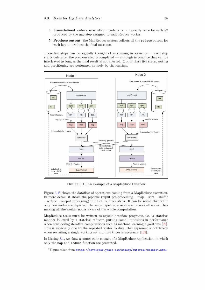
3.3. Tools for Big Data Analytics 35
4. User-defined reduce execution: reduce is run exactly once for each k2produced by the map step assigned to each Reduce worker.
5. Produce output: the MapReduce system collects all the reduce output foreach key to produce the final outcome.
These five steps can be logically thought of as running in sequence — each stepstarts only after the previous step is completed — although in practice they can beinterleaved as long as the final result is not affected. Out of these five steps, sortingand partitioning are performed natively by the runtime.
Figure 3.1: An example of a MapReduce Dataflow
Figure 3.13 shows the dataflow of operations coming from a MapReduce execution.In more detail, it shows the pipeline (input pre-processing – map – sort – shuffle– reduce – output processing) in all of its inner steps. It can be noted that whileonly two nodes are depicted, the same pipeline is replicated across all nodes, thusmaking all the worker nodes aware of the whole computation.
MapReduce tasks must be written as acyclic dataflow programs, i.e. a statelessmapper followed by a stateless reducer, putting some limitations in performancewhen considering iterative computations such as machine learning algorithms [99].This is especially due to the repeated writes to disk, that represent a bottleneckwhen revisiting a single working set multiple times is necessary [132].
In Listing 3.1, we show a source code extract of a MapReduce application, in whichonly the map and reduce function are presented.
3Figure taken from https://developer.yahoo.com/hadoop/tutorial/module4.html

36 Chapter 3. Overview of Big Data Analytics Tools
1 public class WordCount {
2 public static class TokenizerMapper extends Mapper<Object,Text,Text,
IntWritable>{
3 private final static IntWritable one = new IntWritable(1);
4 private Text word = new Text();
5
6 public void map(Object key, Text value, Context context) throws IOException,
InterruptedException{
7 StringTokenizer itr = new StringTokenizer(value.toString());
8 while (itr.hasMoreTokens()) {
9 word.set(itr.nextToken());
10 context.write(word, one);
11 }
12 }
13 }
14 }
15
16 public static class IntSumReducer extends Reducer<Text,IntWritable,Text,
IntWritable> {
17 private IntWritable result = new IntWritable();
18 public void reduce(Text key, Iterable<IntWritable> values, Context context)
throws IOException, InterruptedException {
19 int sum = 0;
20 for (IntWritable val : values) {
21 sum += val.get();
22 }
23 result.set(sum);
24 context.write(key, result);
25 }
26 }
Listing 3.1: The map and reduce functions for a JavaWord Count class example in MapReduce.
3.3.2 Microsoft Dryad
Dryad [79] is a Microsoft research framework for distributed processing of coarse-grain data parallel applications. A Dryad application is a Dataflow graph wherecomputational vertexes are connected among each other with communication chan-nels. Dryad runs the application by executing the graph’s vertexes on a set ofavailable computers, communicating through files, TCP pipes, and shared-memoryFIFO queues. Kernel functions executed by the vertexes are sequential functions(with no threads creation or data contention) provided by the user. Concurrencyarises from scheduling vertexes to run simultaneously on shared memory or on dis-tributed systems. A Dryad application developer can specify an arbitrary directedacyclic graph to describe the application’s communication patterns, and express thedata transport mechanisms (files, TCP pipes, and shared memory FIFO queues)between the computation vertexes. Dryad is notable for allowing graph vertexesto use an arbitrary number of inputs and outputs, while MapReduce restricts allcomputations to take a single input set and generate a single output set. AlthoughDryad provides a nice alternative to MapReduce, Microsoft terminated developmenton Dryad in 2011.
A Dryad application DAG
In Dryad, graphs are created by combining subgraphs or by using simple vertexes. Agraph is formally defined as a tuple G = 〈VG, EG, IG, OG〉 where VG and EG are setof vertexes and edges, while IG ⊆ VG and OG ⊆ VG are input and output vertexes,respectively. No graph can contain edges entering an input vertex nor can containedges exiting an output vertex. Edges are created in two ways: 1) by applying acomposition of two existing graphs (a single vertex is considered a graph), and 2) by

3.3. Tools for Big Data Analytics 37
merging graphs by the union of their vertexes and edges. Edges represent channels.By default, channels are implemented as temporary files where the producer vertexwrites to and the producer vertex reads from. Users can even choose to use channelimplemented as shared memory FIFO queues or TCP channels. Once created, aDryad DAG is optimized using various heuristics. The Dryad runtime parallelizesthe application graph by distributing the computational vertexes across variousexecution engines (in shared memory or shared nothing). Note that replicatingthe whole application graph is also a valid distribution, to exploit data parallelism.Scheduling of the computational vertexes on the available hardware is handled bythe runtime.
3.3.3 Microsoft Naiad
Naiad is an investigation of data-parallel dataflow computation, successor of Dryad,focusing on low-latency streaming and cyclic computations [96]. Naiad’s authorsintroduced a new computational model called Timely Dataflow, which enrichesdataflow computation with timestamps that represent logical points in the com-putation. This model provides the user with the possibility of implementing itera-tive computations, thanks to feedback loops in the dataflow. Stateful nodes in thedataflow can manage a global status for coordination: they asynchronously receivemessages and notifications of global progress, used also in loop management.
Timely Dataflow and Naiad programming model
Timely Dataflow is a model of data-parallel computation that extends traditionaldataflow by associating each communication event with a virtual time that does notneed to be ordered. As in the Time Warp mechanism [81], virtual times serve todifferentiate between data in different phases or aspects of a computation, for exam-ple, data associated with different batches of inputs and different loop iterations.A formal definition of Timely Dataflow can be found in [3]. In this model, eachnode may request different notifications about completions for loops, for instance,thus allowing asynchronous processing. Timely Dataflow graphs are directed graphswhere vertexes are organized into possibly nested loop contexts. Edges entering aloop context must pass through an ingress vertex and edges leaving a loop contextmust pass through an egress vertex. Additionally, every cycle in the graph mustbe contained entirely within some loop context, and must include at least one feed-back vertex that is not nested within any inner loop context. Every token flowingon edges carries a timestamp of the form Timestamp := (e ∈ N, 〈 c1, . . . cn〉 ∈ Nk).The value e represents an epoch, corresponding to integer timestamp representingthe id of the item within the stream, while k is the depth of nesting in a timestamphaving k ≥ 0 loop counters.
The programming model is quite straightforward: a Naiad program is implementedby means of Dataflow nodes created by extending the Vertex<T> interface. Suchvertex is a possibly stateful object that sends and receives messages, and requestsand receives notifications. Message exchange and notification delivery are asyn-chronous. Vertexes can modify arbitrary state in their callbacks, and send mes-sages on any of their outgoing edges. Parallelism is obtained by creating multipleinstances of some vertexes, thus exploiting data parallelism in operators, inter-operators parallelism and loop parallelism. A Naiad application may be run onshared memory and on distributed systems. The smallest unit of computation isthe Worker, namely a single thread, called a shard. Processes are larger unit ofcomputation, which may contain one or more Workers (thus executing one or morevertexes). A single machine may host one or more processes.
Listing 3.2 presents a code fragment implementing a MapReduce style computation.

38 Chapter 3. Overview of Big Data Analytics Tools
1 // 1a. Define input stages for the dataflow.
2 var input = controller.NewInput<string>();
3
4 // 1b. Define the timely dataflow graph.
5 var result = input.SelectMany(y => map(y))
6 .GroupBy(y => key(y), (k, vs) => reduce(k, vs));
7
8 // 1c. Define output callbacks for each epoch
9 result.Subscribe(result => { ... });
10
11 // Step 2. Supply input data to the query.
12 input.OnNext(/* 1st epoch data */);
13 input.OnNext(/* 2nd epoch data */);
14 input.OnNext(/* 3rd epoch data */);
15 input.OnCompleted();
Listing 3.2: A LINQ MapReduce computationexample in Naiad (taken from [96]).
Step 1a defines the source of data, and Step 1c defines what to do with output datawhen produced. Step 1b constructs a Timely Dataflow graph using SelectMany
and GroupBy library calls, which are pre-defined vertexes. SelectMany applies itsargument function to each message (thus it is a map function), and GroupBy groupsresults by a key function before applying its reduction function reduce. Once thegraph is built, in step 2 OnNext supplies the computation with epochs of inputdata. The Subscribe stage applies its callback to each completed epoch of datait observes. Finally, OnCompleted indicates that no further epochs of input dataexist, so the runtime can drain messages and shut down the computation.
3.3.4 Apache Spark
As mentioned in previous sections, MapReduce is not suitable for iterative algo-rithms or interactive analytics, not because it is not possible to implement iterativejobs, but because data have to be repeatedly stored and loaded at each iteration.Furthermore, data can be replicated on the distributed file system between succes-sive jobs. Apache Spark [133, 131, 132] design is intended to solve this problemby reusing the working dataset by keeping it in memory, For this reason, Sparkrepresents a landmark in Big Data tools history, having a strong success in the com-munity. The overall framework and parallel computing model of Spark is similar toMapReduce, while the innovation is in the data model, represented by the ResilientDistributed Dataset (RDD), which are immutable multisets. In this Section, weonly give an overview of Spark, which will be further investigated in Chapter 4.
A Spark program can be characterized by the two kinds of operations applicable toRDDs: transformations and actions. Those transformations and actions composethe directed acyclic graph (DAG) representing the application. Transformationsare the functional style operations applicable to collections, such as map, reduce,flatmap, that are uniformly applied to whole RDDs [131]. Actions return a value tothe user after running a computation on the dataset, thus they effectively start theprogram execution. Transformations in Spark are lazy, in that they do not computetheir results right away. Instead, they just store the transformations applied to somebase dataset, and they are computed when an action requires a result to be returnedto the driver program, that is, the main program written by the programmer.

3.3. Tools for Big Data Analytics 39
Listing 3.3 shows the source code for a simple Word Count application in the JavaSpark API.
1 JavaRDD<String> textFile=sc.textFile("hdfs://...");
2
3 JavaRDD<String> words =
4 textFile.flatMap(new FlatMapFunction<String, String>() {
5 public Iterable<String> call(String s) {
6 return Arrays.asList(s.split(" "));
7 }
8 });
9
10 JavaPairRDD<String, Integer> pairs =
11 words.mapToPair(new PairFunction<String, String, Integer>() {
12 public Tuple2<String, Integer> call(String s) {
13 return new Tuple2<String, Integer>(s, 1);
14 }
15 });
16
17 JavaPairRDD<String, Integer> counts =
18 pairs.reduceByKey(new Function2<Integer, Integer, Integer>() {
19 public Integer call(Integer a, Integer b) {
20 return a + b;
21 }
22 });
23 counts.saveAsTextFile("hdfs://...");
Listing 3.3: A Java Word Count example in Spark.
For stream processing, Spark implements an extension through the Spark Stream-ing module, providing a high-level abstraction called discretized stream or DStream[133]. Such streams represent results in continuous sequences of RDDs of the sametype, called micro-batch. Spark’s execution model relies on the Master-Workermodel: a cluster manager (e.g., YARN) manages resources and supervises the ex-ecution of the program. It manages application scheduling to worker nodes, whichexecute the application logic (the DAG) that has been serialized and sent by themaster.
Resilient Distributed Datasets
An RDD is a read-only collection of objects partitioned across a cluster of computersthat can be operated on in parallel. A Spark application consists of a driver programthat creates RDDs from, for instance, HDFS files or an existing Scala collectionas well as creating RDDs from queries to databases. The driver program maytransform an RDD in parallel by invoking supported operations with user-definedfunctions, which returns another RDD. Since RDDs are read-only collections, eachtransformation on such collections creates a new RDD containing the result of thetransformation. This new collection is not materialized, nor kept in memory: it isthe result of an expression rather than a value and it is computed each time thetransformation is called. The driver can also persist an RDD in memory, allowingit to be reused efficiently across parallel operations without recomputing it. In fact,the semantics of RDDs have the following properties:
• Abstract: elements of an RDD do not have to exist in physical memory. Inthis sense, an element of an RDD is an expression rather than a value. Thevalue can be computed by evaluating the expression when necessary (i.e.,when executing an action).
• Lazy and Ephemeral: RDDs can be created from a file or by transformingan existing RDD such as map, filter, groupByKey, reduceByKey, join, etc.However, RDDs are materialized on demand when they are used in someoperation, and are discarded from memory after use. This thus performs asort of lazy evaluation.

40 Chapter 3. Overview of Big Data Analytics Tools
• Caching and Persistence: a dataset can be cached in memory across oper-ations, which allows future actions to be much faster since they not haveto be reconstructed. Caching is a key tool for iterative algorithms and fastinteractive use cases and it is actually one special case of persistence that al-lows different storage levels, e.g. persisting the dataset on disk or in memorybut as serialized Java objects (to save space), replicating it across nodes, orstoring it off-JVM heap.
• Fault Tolerance: if any partition of an RDD is lost, the lost block will auto-matically be recomputed using only the transformations that originally cre-ated it.
The operations on RDDs take user-defined functions, which are considered closuresin functional programming style features provided by the Scala programming lan-guage, used to implement the Spark runtime. A closure can refer to variables inthe scope when created, which will be copied to the workers when Spark runs aclosure. We recall that, exploiting the JVM and serialization features, it is possibleto serialize closures and send them to Workers.
Operations on RDDs take user-defined functions as arguments, which act as closuresthat can refer to non-local variables from the scope where they were created. Thesecaptured variables will be copied to the workers when Spark runs a closure. Werecall that, exploiting the JVM and serialization features, it is possible to serializeclosures and send them to workers.
Spark also offers two kinds of shared variables:
• Broadcast variables, which are copied to the workers once, and appropriatewhen large read-only data is used in multiple operations
• Accumulators, which are states local to Workers that are only “updated”through an associative operation and can therefore be efficiently supportedin parallel. Accumulators can thus be used to implement counters or sums.Only the driver program can read the accumulator’s value. Spark nativelysupports accumulators of numeric types.
By reusing cached data in RDDs, Spark offers great performance improvement overHadoop MapReduce [131], thus making it suitable for iterative machine learningalgorithms. Similar to MapReduce, Spark is independent of the underlying storagesystem. It is the application developer’s duty to organize data on distributed nodes— i.e., by partitioning and collocating related datasets, etc. — if a distributedfile system is not available. These are critical for interactive analytics, since justcaching is insufficient and not effective for extremely large data.
Spark Streaming
For stream processing, Spark implements an extension through the Spark Streamingmodule, providing a high-level abstraction called discretized stream or DStream[133]. Such streams represent results in continuous sequences of RDDs of the sametype, called micro-batch. Operations over DStreams are “forwarded” to each RDDin the DStream, thus the semantics of operations over streams is defined in termsof batch processing according to the simple translation op(a) = [op(a1), op(a2), . . .],where [·] refers to a possibly unbounded ordered sequence, a = [a1, a2, . . .] is aDStream, and each item ai is a micro-batch of type RDD. All RDDs in a DStreamare processed in order, whereas data items inside an RDD are processed in parallelwithout any ordering guarantees.

3.3. Tools for Big Data Analytics 41
3.3.5 Apache Flink
Formerly known as Stratosphere [21], Apache Flink [42] focuses on stream program-ming. The abstraction used is the DataStream, which is a representation of a streamas a single object. Operations are composed (i.e, pipelined) by calling operators onDataStream objects. Flink also provides the DataSet type for batch applications,that identifies a single immutable multiset—a stream of one element. A Flink pro-gram, either for stream or batch processing, is a term from an algebra of operatorsover DataStreams or DataSets, respectively.
Flink, differently from Spark, is a stream processing framework, meaning that bothbatch and stream processing are based on a streaming runtime. It can be consid-ered one of the more advanced stream processors as many of its core features werealready considered in the initial design [42]. A strong attention is put on providingexactly-once processing guarantee, reached by implementing an algorithm based onChandy-Lamport algorithm for distributed snapshots [44]. In this algorithm, water-mark items are periodically injected into the data stream and trigger any receivingcomponent to create a checkpoint of its local state. On success, all local checkpointsfor a given watermark comprise a distributed global system checkpoint. In a failurescenario, all components are reset to the last valid global checkpoint and data isreplayed from the corresponding watermark. Since data items may never overtakewatermark items, acknowledgment does not happen on a per-item basis.
Other aspects of Flink will be further investigated in Chapter 4.
Flink Programming and Execution Model
Flink adopts a programming model similar to Spark, in which operations are appliedto datasets and streams in a object oriented fashion. The basic building blocks arestreams and transformations (note that a DataSet is internally also a stream). Astream is an intermediate result, and a transformation is an operation that takesone or more streams as input, and computes one or more result streams.
Listing 3.4 shows Flink’s source code for the simple Word Count application.
1 public class WordCountExample {
2 public static void main(String[] args) throws Exception {
3 final ExecutionEnvironment env =
4 ExecutionEnvironment.getExecutionEnvironment();
5 DataSet<String> text = env.fromElements("Text...");
6 DataSet<Tuple2<String, Integer>> wordCounts =
7 text.flatMap(new LineSplitter())
8 .groupBy(0)
9 .sum(1);
10
11 wordCounts.print();
12 }
13
14 public static class LineSplitter
15 implements FlatMapFunction<String, Tuple2<String, Integer>> {
16 @Override
17 public void flatMap(String line,
18 Collector<Tuple2<String, Integer>> out) {
19 for (String word : line.split(" ")) {
20 out.collect(new Tuple2<String, Integer>(word, 1));
21 }
22 }
23 }
24 }
Listing 3.4: A Java Word Count example in Flink.
Flink programs are mapped to streaming dataflows, consisting of streams and trans-formation operators that build arbitrary directed acyclic graphs (DAGs). Each

42 Chapter 3. Overview of Big Data Analytics Tools
dataflow starts with one or more sources and ends in one or more sinks. Specialforms of cycles are permitted via iteration constructs that are discussed in Sec-tion 4.2.3.
Flink’s execution model relies on the Master-Worker model: a deployment has atleast one job manager process that coordinates checkpointing, recovery, and thatreceives Flink jobs. The job manager also schedules work across the task managerprocesses (i.e. workers) which usually reside on separate machines and in turnexecute the code. For distributed execution, Flink optimizes the DAG by chainingoperator subtasks together into tasks: it reduces the overhead of thread-to-threadhandover and buffering, and increases overall throughput while decreasing latency.Stateful stream operators are discussed in Section 4.2.3.
3.3.6 Apache Storm
Apache Storm [97, 117, 126] is a framework targeting only stream processing. It isperhaps the first widely used large-scale stream processing framework in the opensource world. Storm’s programming model is based on three key notions: Spouts,Bolts, and Topologies. A Spout is a source of a stream, that is (typically) connectedto a data source or that can generate its own stream. A Bolt is a processing element,so it processes any number of input streams and produces any number of new outputstreams. Most of the logic of a computation goes into Bolts, such as functions,filters, streaming joins or streaming aggregations. A Topology is the compositionof Spouts and Bolts resulting in a network. Storm uses tuples as its data model,that is, named lists of values of arbitrary type. Hence, Bolts are parametrized withper-tuple kernel code. Each time a tuple is available from some input stream, thekernel code gets activated to work on that input tuple. Bolts and Spouts are locallystateful, as we discuss in Section 4.2.3, while no global consistent state is supported.Globally stateful computations can be implemented since the kernel code of Spoutsand Bolts is arbitrary. However, eventual global state management would be thesole responsibility of the user, who has to be aware of the underlying executionmodel in order ensure program coordination among Spouts and Bolts. It is alsopossible to define cyclic graphs by way of feedback channels connecting Bolts.
While Storm targets single-tuple granularity in its base interface, the Trident API isan abstraction that provides declarative stream processing on top of Storm. Namely,Trident processes streams as a series of micro-batches belonging to a stream consid-ered as a single object. Listing 3.5 show Storm’s source code for the simple WordCount application.

3.3. Tools for Big Data Analytics 43
1 public class WordCountTopology {
2 public static class SplitSentence extends ShellBolt implements IRichBolt {
3 public SplitSentence() {
4 super("python", "splitsentence.py");
5 }
6
7 @Override
8 public void declareOutputFields(OutputFieldsDeclarer declarer) {
9 declarer.declare(new Fields("word"));
10 }
11
12 @Override
13 public Map<String, Object> getComponentConfiguration() {
14 return null;
15 }
16 }
17
18 public static class WordCount extends BaseBasicBolt {
19 Map<String, Integer> counts = new HashMap<String, Integer>();
20
21 @Override
22 public void execute(Tuple tuple, BasicOutputCollector collector) {
23 String word = tuple.getString(0);
24 Integer count = counts.get(word);
25 if (count == null) count = 0;
26 count++;
27 counts.put(word, count);
28 collector.emit(new Values(word, count));
29 }
30
31 @Override
32 public void declareOutputFields(OutputFieldsDeclarer declarer) {
33 declarer.declare(new Fields("word", "count"));
34 }
35 }
36
37 public static void main(String[] args) throws Exception {
38 TopologyBuilder builder = new TopologyBuilder();
39 builder.setSpout("spout", new RandomSentenceSpout(), 5);
40 builder.setBolt("split", new SplitSentence(), 8).shuffleGrouping("spout");
41 builder.setBolt("count", new WordCount(), 12).fieldsGrouping("split", new
Fields("word"));
42 Config conf = new Config();
43 conf.setDebug(true);
44 conf.setNumWorkers(3);
45 StormSubmitter.submitTopology(args[0], conf, builder.createTopology());
46 }
47
Listing 3.5: A Java Word Count example in Storm.
Tasks and Grouping
The execution of each and every Spout and Bolt by Storm is called a Task, whichis the smallest logical unit of a Topology. In simple words, a Task is either theexecution of a Spout or a Bolt. At a given time, each Spout and Bolt can havemultiple instances running in multiple separate threads. The execution model inStorm is based on a Master-Worker paradigm, in which Workers receive Tasks fromthe runtime. Apache Storm has two type of nodes, Nimbus (master node) and Su-pervisor (worker node). Nimbus is the central component of Apache Storm, runningthe Storm Topology. Nimbus analyzes the Topology and gathers the tasks to be ex-ecuted. Then, it distributes each task to an available supervisor. A Supervisor willhave one or more worker processes to which it delegates Tasks. Worker processeswill spawn as many executors as needed and run the task. Apache Storm uses aninternal distributed messaging system for the communication between Nimbus andSupervisors.

44 Chapter 3. Overview of Big Data Analytics Tools
Stream grouping controls how the tuples are routed in the Topology. There are fourmain built-in groupings:
• Shuffle Grouping: tuples are randomly distributed across the Bolt’s tasks sothat each Bolt is guaranteed to get an equal number of tuples
• Field Grouping: this performs a tuple partitioning, in which tuples with thesame field values are sent forward to the same worker executing the bolts
• Global Grouping: all the streams can be grouped and forwarded to one Bolt.This grouping sends tuples generated by all instances of the source to a singletarget instance.
• All Grouping: sends a single copy of each tuple to all instances of the receivingbolt. This kind of grouping is used to send signals to Bolt (i.e., broadcast).
3.3.7 FlumeJava
FlumeJava [43] is a Java library developed by Google for data-parallel pipelines. Itcan be considered the ancestor of Google Dataflow. Its core is centered on paralleloperators on parallel collections: internally, it implements parallel operations usingdeferred evaluation, thus the invocation of a parallel operation is stored with itsarguments in an internal execution plan graph structure. Once the execution planfor the whole computation has been constructed, FlumeJava optimizes the executionplan by, for example, fusing chains of parallel operations together into a smallnumber of MapReduce operations. FlumeJava supports only batch execution andwith a Bulk-synchronous model: the runtime executor traverses the operations inthe execution plan in forward topological order, executing each one in turn. Thesame program can execute completely locally when run on small inputs and usingmany parallel machines when run on large inputs.
Data Model and Transformations
In FlumeJava, there are several classes representing different data. The core ab-straction for representing data is the PCollection, containing ordered as well asunordered data. The second core abstraction is the PTable, representing data inthe form of key-value pairs, where the value is always a PCollection. PCollectionsare transformed via parallel operations, such as parallelDo (i.e., map) or join,for instance. Those parallel operations are executed lazily. Each PCollection objectis represented internally with a deferred (not yet computed) or materialized (com-puted) state. A deferred PCollection holds a pointer to the deferred operation thatcomputes it, holding references to the PCollections that are its arguments (whichmay themselves be deferred or materialized) and the deferred PCollections that areits results. When a FlumeJava operation like parallelDo() is called, it creates aParallelDo deferred operation object and returns a new deferred PCollection thatpoints to it. The result of executing a series of FlumeJava operations is thus adirected acyclic graph of deferred PCollections and operations, called the execu-tion plan. The execution plan is visited by the internal optimizer with the goal ofproducing the most efficient execution plan.
One of the most important operations is the MapShuffleCombineReduce (MSCR), inwhich FlumeJava optimizer transforms combinations of ParallelDo, GroupByKey,CombineValues, and Flatten operations into single MapReduce step. It extendsMapReduce by allowing multiple reducers and combiners. Furthermore it allowseach reducer to produce multiple outputs, by removing the requirement that areducer must produce outputs with the same key as the reducer input, and byallowing pass-through outputs, thereby making it a better target for the optimizer,which improves communication patterns.

3.3. Tools for Big Data Analytics 45
The code shown in Listing 3.6 presents a word count example in Apache Crunch [52],the Java library for creating FlumeJava pipelines.
1 public class WordCount {
2 public static void main(String[] args) throws Exception {
3 // Create an object to coordinate pipeline creation and execution.
4 Pipeline pipeline = new MRPipeline(WordCount.class);
5
6 // Reference a given text file as a collection of Strings.
7 PCollection<String> lines = pipeline.readTextFile(args[0]);
8
9 // Define a function that splits each line in a PCollection of Strings
10 // into a PCollection made up of the individual words in the file.
11 PCollection<String> words = lines.parallelDo(
12 new DoFn<String, String>() {
13 public void process(String line, Emitter<String> emitter) {
14 for (String word : line.split("\\s+")) {
15 emitter.emit(word);
16 }
17 }
18 },
19 Writables.strings() // Indicates the serialization format
20 );
21
22 // The count method applies a series of Crunch primitives and returns a
23 // map of the top 20 unique words in the input PCollection to their counts.
24 // We then read the results of the MapReduce jobs that performed the
25 // computations into the client and write them to stdout.
26 for (Pair<String, Long> wordCount: words.count().top(20).materialize()) {
27 System.out.println(wordCount);
28 }
29 }
30 }
Listing 3.6: A Complete Java Word Count example inCrunch API for FlumeJava.
3.3.8 Google Dataflow
Google Dataflow SDK [6] is part of the Google Cloud Platform [72]. Here, “Dataflow”is used refering to the “Dataflow model” to describe the processing and program-ming model of the Cloud Platform. This framework aims to provide a unified modelfor stream, batch and micro-batch processing. It is built based on four major con-cepts:
• Pipelines
• PCollections
• Transforms
• I/O Sources and Sinks
The base entity is the Pipeline, representing a data processing job consisting of aset of operations that can read a source of input data, transform that data, andwrite out the resulting output. The data and transforms in a pipeline are uniqueto, and owned by, that Pipeline, while multiple Pipelines cannot share data ortransforms. A Pipeline can be linear but it can also branch and merge, thus makinga Pipeline a directed graph of steps and its construction can create this directedgraph by using conditionals, loops, and other common programming structures. Itis possible to implement iterative algorithms only if a fixed and known number ofiterations is provided, while it may not be easy to implement algorithms wherethe Pipeline’s execution graph depends on the data itself. This happens becauseof the computation graph which is built in an intermediate language that is then

46 Chapter 3. Overview of Big Data Analytics Tools
optimized before being executed. With iterative algorithms, the complete graphstructure cannot be known beforehand, so it is necessary to know the number ofiteration in advance in order to replicate the subset of stages in the pipeline involvedin the iterative step.
The DAG resulting from a Pipeline is optimized and compiled into a language-agnostic representation before execution.
The execution of a Dataflow program is typically launched on the Google CloudPlatform. When run, Dataflow runtime enters the Graph Construction Time phasein which it creates an execution graph on the basis of the Pipeline, including allthe Transforms and processing functions. The execution graph is translated intoJSON format and it transmitted to the Dataflow service endpoint. Once validated,this graph is translated into a job on the Dataflow service, which automaticallyparallelizes and distributes the processing logic to the workers allocated by the userto perform the job.
Data Model and Transformations
A PCollection represents a potentially large, immutable bag of elements, that canbe either bounded or unbounded. Elements in a PCollection can be of any type, butthe type must be consistent. However, the user must provide the runtime with theencoding of the data type as a byte string in order to serialize and send data amongdistributed processing units. Dataflow’s Transforms use PCollections, that is, itis the only abstract data type accepted by operations. Each PCollection is localto a specific Pipeline object and has the following properties: 1) It is immutable;each transformation instantiates a new PCollection. 2) It does not support randomaccess to individual elements and, 3) A PCollection is private to a Pipeline.
The bounded (or unbounded) nature of a PCollection affects how Dataflow processesthe data. Bounded PCollections can be processed using batch jobs, that mightread the entire data set once, and perform processing in a finite job. UnboundedPCollections must be processed using streaming jobs, as the entire collection cannever be available for processing at any one time and they can be grouped by usingwindowing to create logical windows of finite size.
A Transform represents an operation on PCollections, that is, it is a stage of thePipeline. It accepts one (or multiple) PCollection(s) as input, performs an operationon the elements in the input PCollection(s), and produces one (or multiple) newPCollection(s) as output. Transforms are applied to an input PCollection by callingthe apply method on that collection. The output PCollection is the value returnedfrom PCollection.apply.

3.3. Tools for Big Data Analytics 47
For example, Listing 3.7 shows how to create a Word Count Pipeline.
1 public static void main(String[] args) {
2 // Create a pipeline parameterized by commandline flags.
3 Pipeline p = Pipeline.create(PipelineOptionsFactory.fromArgs(arg));
4 //The Count transform below returns a new PCollection of key/value
5 //pairs, where each key represents a unique word in the text.
6
7 p.apply(TextIO.Read.from("gs://...")) // Read input.
8 .apply(ParDo.named("ExtractWords").of(new DoFn<String, String>() {
9 @Override
10 public void processElement(ProcessContext c) {
11 for (String word : c.element().split("[^a-zA-Z’]+")) {
12 if (!word.isEmpty()) {
13 c.output(word);
14 }
15 }
16 }
17 }))
18 .apply(Count.<String>perElement())
19 .apply("FormatResults",
20 MapElements.via(new SimpleFunction<KV<String, Long>, String>() {
21 @Override
22 public String apply(KV<String, Long> input) {
23 return input.getKey() + ": " + input.getValue();
24 }
25 }))
26 .apply(TextIO.Write.to("gs://...")); // Write output.
27
28 // Run the pipeline.
29 p.run();
30 }
Listing 3.7: Java code fragment for a Word Countexample in Google Dataflow.
The ParDo is the core element-wise transform in Google Dataflow, invoking a user-specified function on each of the elements of the input PCollection to produce zeroor more output elements (flatmap semantics) collected into an output PCollection.Elements are processed independently, possibly in parallel across distributed cloudresources.
When executing a ParDo transform, the elements of the input PCollection are firstdivided up into a certain number of “bundles” (which can be considered like micro-batches). These are farmed off to distributed worker machines (or run locally). Foreach bundle of input elements, processing proceeds as follows:
1. A fresh instance of the argument DoFn (namely the class argument of theParDo transform) is created on a worker (through deserialization or othermeans).
2. The DoFn’s startBundle method is called to initialize the bundle, if overridden.
3. The DoFn’s processElement method is called on each of the input elements inthe bundle.
4. The DoFn’s finishBundle method is called to complete its work, if overridden.
The ParDo can take also additional “side input”, that is a state local to the ParDo
instance or a broadcast value.
Google Dataflow will be further investigated in Chapter 4.
3.3.9 Thrill
Thrill [34] is a prototype of a general purpose big data batch processing frameworkwith a data-flow style programming interface implemented in C++ and exploiting

48 Chapter 3. Overview of Big Data Analytics Tools
template meta-programming. Thrill uses arrays rather than multisets as its primarydata structure to enable operations like sorting, prefix sums, window scans, orcombining corresponding fields of several arrays (zipping). Thrill programs run ina collective bulk-synchronous manner similar to most MPI programs, focusing onfast in-memory computation, but transparently uses external memory when needed.The functional programming style used by Thrill enables easy parallelization, whichalso works well for shared memory parallelism. A consequence of using C++ is thatmemory management has to be done explicitly. However, memory management inmodern C++11 has been considerably simplified, and Thrill uses reference countingextensively. Thrill’s authors wanted to emphasize that, with the advent of C++11lambda-expressions, it has become easier to use C++ for big data processing usingan API comparable to currently popular frameworks like Spark or Flink.
Thrill execution model is similar to MPI programs, where the same program is runon different machines, i.e., SPMD (Single Program, Multiple Data). The binary isexecuted simultaneously on all machines and communication supports TCP socketsand MPI. Each machine is called a host and each thread on a host is called a worker.There is no master or driver host, as all communication is done collectively.
Distributed Immutable Arrays
Thrill’s data model is based on distributed immutable array (DIA). A DIA is an arrayof items distributed over the cluster, to which no direct access is permitted, that is,it is only possible to apply operations to the array as a whole. In a Thrill program,these operations are used to lazily construct a DIA data-flow graph in C++, asshown in Listing 3.8. The data-flow graph is only executed when an action operationis encountered. How DIA items are actually stored and in what way the operationsare executed on the distributed system remains transparent to the user. In thecurrent Thrill prototype, the array is usually distributed evenly among workers, inorder. DIAs can contain any C++ data type, provided serialization methods areavailable. Thrill provides built-in serialization methods for all primitive types andmost STL types; only custom non-trivial classes require additional methods. EachDIA operation is implemented as a C++ template class.
1 void WordCount(thrill::Context& ctx, std::string input, std::string output) {
2 using Pair = std::pair<std::string, size_t>;
3 auto word_pairs = ReadLines(ctx, input).template FlatMap<Pair>(
4 // flatmap lambda: split and emit each word
5 [](const std::string& line, auto emit) {
6 Split(line, ’ ’, [&](std::string_view sv) {
7 emit(Pair(sv.to_string(), 1));
8 });
9 });
10 word_pairs.ReduceByKey(
11 // key extractor: the word string
12 [](const Pair& p) { return p.first; },
13 // commutative reduction: add counters
14 [](const Pair& a, const Pair& b) { return Pair(a.first, a.second + b.second)
; }
15 )
16 .Map([](const Pair& p) { return p.first + ": " + std::to_string(p.second); })
17 .WriteLines(output);
18 }
Listing 3.8: A C++ complete Word Count example inThrill.
The immutability of a DIA enables functional-style dataflow programming. As DIAoperations can depend on other DIAs as inputs, these form a directed acyclic graph(DAG), which is called the DIA dataflow graph, where vertexes represent operationsand directed edges represent data dependencies.

3.3. Tools for Big Data Analytics 49
A DIA remains purely an abstract dataflow between two concrete DIA operations,allowing to apply optimizations such as pipelining or chaining, combining the logicof one or more functions into a single one (called pipeline). All independentlyparallelizable local operations (e.g., FlatMap, Map) and the first local computationsteps of the next distributed DIA operation are packed into one block of optimizedbinary code. Via this chaining, it is possible to reduce the data movement overheadas well as the total number of operations that need to store intermediate arrays.
3.3.10 Kafka
Apache Kafka [87] is an open-source stream processing platform implemented inScala and Java, aiming to provide a unified, high-throughput, low-latency platformfor handling real-time data feeds. Kafka is based on a producer-consumer modelexchanging streams of messages. Each stream of messages of a particular type iscalled a topic: a producer can publish messages to a topic, which are then storedat a set of servers called brokers, while a consumer can subscribe to one or moretopics from the brokers, and consume the subscribed messages by pulling data fromthe brokers. A feature of Kafka is that each message stream provides an iteratorinterface over the stream produced. The consumer can iterate over every messagein the stream and, unlike traditional iterators, the message stream iterator neverterminates and exposes a blocking behavior until new messages are published. SinceKafka is distributed, a Kafka cluster typically consists of multiple brokers, hence atopic is divided into multiple partitions and each broker stores one or more of those.A consumer consumes messages from a particular partition sequentially.
Producer-Consumer Distributed Coordination
Each producer can publish a message to either a randomly selected partition or apartition semantically determined by a partitioning key and a partitioning func-tion. Kafka implements the concept of consumer groups consisting of one or moreconsumers having subscribed to a set of topics. Different consumer groups consumeindependently the full set of subscribed messages without communication amonggroups, since they can be in different processes or machines. The consumer starts athread to pull data from each owned partition, starting the iterator over the streamfrom the offset stored in the offset registry. As messages get pulled from a partition,the consumer periodically updates the latest consumed offset in the offset registry.
When there are multiple consumers within a group, each will be notified of a brokeror consumer change. It is possible for a consumer to try to take ownership of apartition still owned by another consumer. In this case, the first consumer releasesall the partitions that it currently owns and retries the re-balance process after acertain timeout.
In this architecture, there is no master node, since consumers coordinates amongthemselves in a decentralized manner.
3.3.11 Google TensorFlow
Google TensorFlow [2] is a framework specifically designed for machine learningapplications, where the data model consists of multidimensional arrays called ten-sors and a program is a composition of operators processing tensors. A TensorFlowapplication is built as a functional-style expression, where each sub-expression canbe given an explicit name. The TensorFlow programming model includes controlflow operations and, notably, synchronization primitives (e.g., MutexAcquire and

50 Chapter 3. Overview of Big Data Analytics Tools
MutexRelease for critical sections). This latter observation implies that Tensor-Flow exposes the underlying (parallel) execution model to the user, who has toprogram the eventual coordination of operators concurring over some global state.TensorFlow allows expressing conditionals and loops by means of specific controlflow operators such as For operator.
Each node has firing rules that depend on the kind of incoming tokens. For example,control dependencies edges can carry synchronization tokens: the target node ofsuch edges cannot execute until all appropriate synchronization signals have beenreceived.
TensorFlow replicates actors implementing certain operators (e.g., tensor multi-plication) on tensors (input tokens). Hence, each actor is a data-parallel actoroperating on intra-task independent input elements—here, multi-dimensional ar-rays (tensors). Moreover, iterative actors/hierarchical actors (in case of cycles ona subgraph) are implemented with tags similar to the MIT Tagged-Token dataflowmachine [28], where the iteration state is identified by a tag and independent it-erations are executed in parallel. In iterative computations, it is worthwhile tounderline that in TensorFlow an input can enter a loop iteration whenever it be-comes available (as in Naiad), instead of imposing barriers after each iteration, asdone, for instance, in Flink.
A TensorFlow application
Listing 3.9 presents a code snippet of a TensorFlow application generating thedataflow graph in figure 3.2. The example computes the rectified linear unit functionfor neural network activations.
1 import tensorflow as tf
2 b = tf.Variable(tf.zeros([100])) # 100-d vector, init to zeroes
3 W = tf.Variable(tf.random_uniform([784,100],-1,1)) # 784x100 matrix w/rnd vals
4 x = tf.placeholder(name="x") # Placeholder for input
5 relu = tf.nn.relu(tf.matmul(W, x) + b) # Relu(Wx+b)
6 C = [...] # Cost as a function of Relu
7 s = tf.Session()
8 for step in xrange(0, 10):
9 input = ...construct 100-D input array ...# Create 100-d vector for input
10 result = s.run(C, feed_dict={x: input}) # Fetch cost, feeding x=input
11 print step, result
Listing 3.9: Example of a Python TensorFlow codefragment in [2].
Figure 3.2: A TensorFlow application graph
Figure 3.2 shows a TensorFlow application graph example from [2]. A node ofthe graph represents a tensor operation, which can also be a data generation one(nodes W , b, x): operators are mapped to actors that take as input single tokens

3.4. Fault Tolerance 51
representing Tensors (multi-dimensional arrays), and are activated once except foriterative computations.
3.3.12 Machine Learning and Deep Learning Frameworks
Besides we described only TensorFlow in our overview, different other Machineand Deep Learning frameworks are present in the community. In the following, weprovide common characteristics from both data and programming model perspectiveof some well known frameworks such as Caffe, Torch and Theano. We do not providea comprehensive list since focusing on Machine and Deep Learning it is out of thescope of this overview. A comparative study of such frameworks can be found inBahrampour et al. work [30].
Caffe [82] is a framework for Deep Learning providing the user with state-of-the-artalgorithms and a collection of reference models. It is implemented in C++ withPython and MATLAB interfaces. Furthermore, it provides support for offload-ing computations on GPUs. Caffe was first designed for vision, but it has beenadopted and improved by users in speech recognition, robotics, neuroscience, andastronomy. Its data model relies on the Blob, a multi-dimensional array used as awrapper over the actual data being processed, providing also synchronization ca-pability between the CPU and the GPU. From an implementation perspective, ablob is an N-dimensional array stored in a C-contiguous fashion. Blobs provide aunified memory interface holding data; e.g., batches of images, model parameters,and derivatives for optimization.
At a higher level, Caffe considers applications as Dataflow graphs. Each programimplements a Deep Network (or simply net): compositional models that are nat-urally represented as a collection of inter-connected layers that work on chunks ofdata. Caffe implements Networks in the concept of net, that is, a set of layers con-nected in a directed acyclic graph (DAG). Caffe does all the bookkeeping for anyDAG of layers to ensure correctness of the forward and backward passes. A typicalnet begins with a data layer that loads from disk and ends with a loss layer thatcomputes the objective for a task such as classification or reconstruction.
Theano [123] is a Python library that allows to define, optimize, and evaluate math-ematical expressions involving multi-dimensional arrays, called tensors, which arethe basic data model for neural network and deep learning programming. Like otherframeworks, it provides support for kernel offloading on GPUs. Its programmingmodel is similar to TensorFlow and, at higher level, applications are represented bydirected acyclic graphs (DAG): these graphs are composed of interconnected Apply,Variable and Op nodes, the latter representing the application of an Op to someVariable.
Torch [51] is a machine learning framework implemented in Lua that runs on Lua(JIT) compiler. Torch implements also CUDA and CPU backends. The core datamodel is represented by Tensors, which extends basic set of types in the Lua pro-gramming language, to provide an efficient multi-dimensional array type. ThisTensor library provides classic operations including linear algebra operations, im-plemented in C, leveraging SSE instructions on Intel platforms. Optionally, it canbind linear algebra operations to existing efficient BLAS/Lapack implementations(like Intel MKL). Torch provides a module for building neural networks using aDataflow based API.
3.4 Fault Tolerance
Fault tolerance is an important aspect to consider when implementing frameworksfor analytics. The main benefits of implementing fault tolerance is to guarantee

52 Chapter 3. Overview of Big Data Analytics Tools
recovery from faults: consider, for instance, when multiple instances of an applica-tion are running and one server crashes for some reason. In this case, the systemmust be able to recover autonomously and consistently from the system failure.Of course, enabling fault tolerance decreases performances of applications. In BigData analytics framework, fault tolerance includes both system failure and datarecovery with checkpointing techniques, but also a software level fault tolerance.The latter is implemented within the framework itself and requires also applicationrecovery from system failure, e.g., a remote worker node crashes and part of thecomputation must be restarted. This guarantees must be confirmed also when run-ning streaming applications. Real-time stream processing systems must be alwaysoperational, which requires them to recover from all kinds of failures in the system,comprehending also the need to store and recover a certain amount of data alreadyprocessed by the streaming application. Consider, for instance, Spark Streamingmanagement of fault tolerance. In a Spark Streaming application, data is usuallyreceived from sources like Kafka and Flume are buffered in the executor’s memoryuntil their processing has completed. If the driver fails, all workers and executorsfails as well, and data can not be recovered even if the driver is restarted. To avoidthis data loss, Write Ahead Logs have been introduced. Write Ahead Logs (alsoknown as a journal) are used in database and file systems to ensure the durabilityof any data operations. The intention of the operation is first stored into a durablelog , and then the operation is applied to the data. If the system fails in the middleof applying the operation, this can recovered and re-executed by reading the log.It worths nothing that such operations at run-time increase the application execu-tion time and decrease performance and resource utilization, but when running ondistributed systems fault tolerance has to be guaranteed.
3.5 Summary
In this Chapter we provided a definition of Big Data and the description of mostcommon tools for analytics and data management. Of course this list is not com-prehensive of all tools, since it would be a very hard task to collect all of them ina single place and it goes beyond the scope of this work. Nevertheless, we believethat the descriptions we provided could be useful to help the reader in having agood overview about the topic and the results of the effort of computer scientistsin the community.

53
Chapter 4
High-Level Model for BigData Frameworks
In this chapter we analyze some well-known tools—Spark, Storm, Flink and GoogleDataflow—and provide a common structure underlying all of them, based on theDataflow model [91] that we identified as the common model that better describes alllevels of abstraction, from the user-level API to the execution model. We instantiatethe Dataflow model into a stack of layers where each layer represents a dataflowgraph/model with a different meaning, describing a program from what is exposedto the programmer down to the underlying execution model layer.
4.1 The Dataflow Layered Model
With the increasing number of Big Data analytics tools, we witness a continu-ous fight among implementors/vendors in demonstrating how their tools are betterthan others in terms of performances and expressiveness. In this hype, for a userapproaching Big Data analytics (even an educated computer scientist), it might bedifficult to have a clear picture of the programming model underneath these toolsand the expressiveness they provide to solve some user defined problem. With thisin mind, we wanted to understand the features those tools provide to the user interms of API and how they are related to parallel computing paradigms.
We use the Dataflow model to describe these tools since it is expressive enoughto describe the batch, micro-batch and streaming models that are implemented inmost tools for Big Data processing. Being all realized under the same common idea,we show how various Big Data analytics tools share almost the same base concepts,differing mostly in their implementation choices.
Furthermore, we put our attention to a problem arising from the high abstractionprovided by the model that reflects into the examined tools. Especially when con-sidering stream processing and state management, non-determinism may arise whenprocessing one or more streams in one node of the graph, which is a well-knownproblem in parallel and distributed computing.
In Section 4.1.1, we outline an architecture that can describe all these models atdifferent levels of abstraction (Fig. 4.1) from the (top) user-level API to the (bottom-level) actual network of processes. In particular, we show how the Dataflow modelis general enough to subsume many different levels only by changing the semanticsof actors and channels.

54 Chapter 4. High-Level Model for Big Data Frameworks
Framework API
Program Semantics Dataflow
Parallel Execution Dataflow
Process Network Dataflow
Platform
User-level API
Semantics of the application in termsof dataflow graphs
Instantiation of semantic dataflowthat explicitly expresses parallelism
Runtime execution model(e.g., Master-Workers)
Runtime language or platform(e.g., JVM)
Figure 4.1: Layered model representing the levels of ab-stractions provided by the frameworks that were analyzed.
4.1.1 The Dataflow Stack
The layered model shown in Fig. 4.1 presents five layers, where the three inter-mediate layers are Dataflow models with different semantics, as described in theparagraphs below. Underneath these three layers is the Platform level, that is, theruntime or programming language used to implement a given framework (e.g., Javaand Scala in Spark), a level which is beyond the scope of our paper. On top is theFramework API level, that describes the user API on top of the Dataflow graph,which will be detailed in Section 4.2. The three Dataflow models in between are asfollows.
• Program Semantics Dataflow : We claim the API exposed by any of the con-sidered frameworks can be translated into a Dataflow graph. The top level ofour layered model captures this translation: programs at this level representthe semantics of data-processing applications in terms of Dataflow graphs.Programs at this level do not explicitly express any form of parallelism: theyonly express data dependencies (i.e., edges) among program components (i.e.,actors). This aspect is covered in Section 4.3.
• Parallel Execution Dataflow : This level, covered in Section 4.4, represents aninstantiation of the semantic dataflows in terms of processing elements (i.e.,actors) connected by data channels (i.e., edges). Independent units—notconnected by a channel—may execute in parallel. For example, a semanticactor can be replicated to express data parallelism, so that the given functioncan be applied to independent input data.
• Process Network Dataflow : This level, covered in Section 4.5, describes howthe program is effectively deployed and executed onto the underlying plat-form. Actors are concrete computing entities (e.g., processes) and edges arecommunication channels. The most common approach is for the actual net-work to be a Master-Workers task executor.
4.2 Programming Models
Data-processing applications are generally divided into batch vs.stream processing.Batch programs process one or more finite datasets to produce a resulting finiteoutput dataset, whereas stream programs process possibly unbounded sequences ofdata, called streams, doing so in an incremental manner. Operations over streams

4.2. Programming Models 55
may also have to respect a total data ordering—for instance, to represent timeordering.
Orthogonally, we divide the frameworks’ user APIs into two categories: declarativeand topological. Spark, Flink and Google Dataflow belong to the first category—they provide batch or stream processing in the form of operators over collections orstreams—whereas Storm, Naiad, Dryad belong to the second one—they providesan API explicitly based on building graphs.
4.2.1 Declarative Data Processing
This model provides building blocks as data collections and operations on those col-lections. The data model follows domain-specific operators, for instance, relationalalgebra operators that operate on data structured with the key-value model.
Declarative batch processing applications are expressed as methods on objects repre-senting collections (e.g. Spark, Google Dataflow and Flink) or as functions on values(e.g. PCollections, in Google Dataflow): these are algebras on finite datasets, whosedata can be ordered or not. APIs with such operations are exposing a functional-likestyle. Here are three examples of operations with their (multiset-based) semantics:1
groupByKey(a) = {(k, {v : (k, v) ∈ a})} (4.1)
join(a, b) = {(k, (va, vb)) : (k, va) ∈ a ∧ (k, vb) ∈ b} (4.2)
map〈f〉(a) = {f(v) : v ∈ a} (4.3)
The groupByKey unary operation groups tuples sharing the same key (i.e., the firstfield of the tuple); thus it maps multisets of type (K × V )∗ to multisets of type(K × V ∗)∗. The binary join operation merges two multisets by coupling valuessharing the same key. Finally, the unary higher-order map operation applies thekernel function f to each element in the input multiset.
Declarative stream processing programs are expressed in terms of an algebra oneventually unbounded data (i.e., stream as a whole) where data ordering eventuallymatters. Data is usually organized in tuples having a key field used for example toexpress the position of each stream item with respect to a global order—a globaltimestamp—or to partition streams into substreams. For instance, this allows ex-pressing relational algebra operators and data grouping. In a stream processingscenario, we also have to consider two important aspects: state and windowing;those are discussed in Section 4.2.3.
Apache Spark implements batch programming with a set of operators, called trans-formations, that are uniformly applied to whole datasets called Resilient DistributedDatasets (RDD) [131], which are immutable multisets. For stream processing, Sparkimplements an extension through the Spark Streaming module, providing a high-level abstraction called discretized stream or DStream [133]. Such streams representresults in continuous sequences of RDDs of the same type, called micro-batch. Op-erations over DStreams are “forwarded” to each RDD in the DStream, thus thesemantics of operations over streams is defined in terms of batch processing ac-cording to the simple translation op(a) = [op(a1), op(a2), . . .], where [·] refers to apossibly unbounded ordered sequence, a = [a1, a2, . . .] is a DStream, and each itemai is a micro-batch of type RDD.
Apache Flink ’s main focus is on stream programming. The abstraction used is theDataStream, which is a representation of a stream as a single object. Operations arecomposed (i.e, pipelined) by calling operators on DataStream objects. Flink alsoprovides the DataSet type for batch applications, that identifies a single immutable
1Here, {·} denotes multisets rather than sets.

56 Chapter 4. High-Level Model for Big Data Frameworks
multiset—a stream of one element. A Flink program, either for stream or batchprocessing, is a term from an algebra of operators over DataStreams or DataSets,respectively. Stateful stream operators and iterative batch processing are discussedin Section 4.2.3.
Google Dataflow [6] provides a unified programming and execution model for stream,batch and micro-batch processing. The base entity is the Pipeline, representing adata processing job consisting of a set of operations that can read a source of inputdata, transform that data, and write out the resulting output. Its programmingmodel is based on three main entities: Pipeline, PCollection and Transformation.Transformations are basically Pipelines’ stages, operating on PCollections, that areprivate to each Pipeline. A PCollection represents a potentially large, immutablebag of elements, that can be either bounded or unbounded. Elements in a PCol-lection can be of any type, but the type must be consistent. One of the mainTransformations in Google Dataflow is the ParDo operation, used for generic par-allel processing. The argument that provided to ParDo must be a subclass of aspecific type provided by the Dataflow SDK, called DoFn. The ParDo takes eachelement in an input PCollection, performs some user defined processing function onthat element, and then emits zero, one, or multiple elements to an output PCollec-tion. The function provided is invoked independently, and in parallel, on multipleworker instances in a Dataflow job.
4.2.2 Topological Data Processing
Topological programs are expressed as graphs, built by explicitly connecting pro-cessing nodes and specifying the code executed by nodes.
Apache Storm is a framework that only targets stream processing. Storm’s pro-gramming model is based on three key notions: Spouts, Bolts, and Topologies. ASpout is a source of a stream, that is (typically) connected to a data source or thatcan generate its own stream. A Bolt is a processing element, so it processes anynumber of input streams and produces any number of new output streams. Mostof the logic of a computation goes into Bolts, such as functions, filters, streamingjoins or streaming aggregations. A Topology is the composition of Spouts and Boltsresulting in a network. Storm uses tuples as its data model, that is, named listsof values of arbitrary type. Hence, Bolts are parametrized with per-tuple kernelcode. Each time a tuple is available from some input stream, the kernel code getsactivated to work on that input tuple. Bolts and Spouts are locally stateful, as wediscuss in Section 4.2.3, while no global consistent state is supported. Yet, glob-ally stateful computations can be implemented since the kernel code of Spouts andBolts is arbitrary. However, eventual global state management would be the soleresponsibility of the user, who has to be aware of the underlying execution model inorder to ensure program coordination among Spouts and Bolts. It is also possibleto define cyclic graphs by way of feedback channels connecting Bolts.
While Storm targets single-tuple granularity in its base interface, the Trident API isan abstraction that provides declarative stream processing on top of Storm. Namely,Trident processes streams as a series of micro-batches belonging to a stream con-sidered as a single object.
4.2.3 State, Windowing and Iterative Computations
Frameworks providing stateful stream processing make it possible to express mod-ifications (i.e., side-effects) to the system state that will be visible at some futurepoint. If the state of the system is global, then it can be accessed by all systemcomponents. Another example of global state is the one managed in Naiad viatagged tokens in their Timely Dataflow model. On the other hand, local states can
4.2. Programming Models 57
be accessed only by a single system component. For example, the mapWithState
functional in the Spark Streaming API realizes a form of local state, in whichsuccessive executions of the functional see the modifications to the state made byprevious ones. Furthermore, state can be partitioned by shaping it as a tuple space,following, for instance, the aforementioned key-value paradigm.
Google Dataflow provides a form of state in the form of side-input, provided asadditional inputs to a ParDo transform. A side input is a local state accessible bythe DoFn object each time it processes an element in the input PCollection. Oncespecified, this side input can be read from within the ParDo transform’s DoFn whileprocessing each element.
Windowing is another concept provided by many stream processing frameworks.A window is informally defined as an ordered subset of items extracted from thestream. The most common form of windowing is referred as sliding window andit is characterized by the size (how many elements fall within the window) andthe sliding policy (how items enter and exit from the window). Spark providesthe simplest abstraction for defining windows, since they are just micro-batchesover the DStream abstraction where it is possible to define only the window lengthand the sliding policy. Storm and Flink allow more arbitrary kinds of grouping,producing windows of Tuples and WindowedStreams, respectively. Notice this doesnot break the declarative or topological nature of the considered frameworks, sinceit just changes the type of the processed data. Notice also that windowing can beexpressed in terms of stateful processing, by considering window-typed state.
Google Dataflow provides three kind of windowing patterns: fixed windows definedby a static window size (e.g. per hour, per second). Sliding windows defined by awindow size and a sliding period. The period may be smaller then the size, to allowoverlapping windows. Session windows capture some period of activity over a subsetof data partitioned by a key. Typically, they are defined by a timeout gap. Whenused with partitioning (e.g., grouping by key), Grouping transforms consider eachPCollection on a per-window basis. GroupByKey, for example, implicitly groupsthe elements of a PCollection by key first and then by window. Windowing canbe used with bounded PCollections, and it considers only the implicit timestampsattached to each element of a PCollection, and data sources that create fixed datasets assign the same timestamp to every element. All the elements are by defaultpart of a single, global window, causing the execution in classic MapReduce batchstyle.
Finally, we consider another common concept in batch processing, namely iter-ative processing. In Flink, iterations are expressed as the composition of ar-bitrary DataSet values by iterative operators, resulting in a so-called Iterative-DataSet. Component DataSets represent for example step functions—executed ineach iteration—or termination condition—evaluated to decide if iteration has to beterminated. Spark’s iteration model is radically simpler, since no specific constructis provided to implement iterative processing. Instead, an RDD (endowed withtransformations) can be embedded into a plain sequential loop. Google Dataflowiteration model is similar to Spark’s but it’s limited. It is possible to implement it-erative algorithms only if a fixed and known number of iterations is provided, whileit may not be easy to implement algorithms where the pipeline’s execution graphdepends on the data itself. This happens because of the computation graph buildin the intermediate language that is then optimized before being executed. Withiterative algorithms, the complete graph structure cannot be known in advance, soit is necessary to know the number of iteration in advance in order to replicate thesubset of stages in the pipeline involved in the iterative step.

58 Chapter 4. High-Level Model for Big Data Frameworks
m rA m(A) b
Figure 4.2: Functional Map and Reduce dataflow express-ing data dependencies.
4.3 Program Semantics Dataflow
This level of our layered model provides a Dataflow representation of the programsemantics. Such a model describes the application using operators and data depen-dencies among them, thus creating a topological view common to all frameworks.This level does not explicitly express parallelism: instead, parallelism is implicitthrough the data dependencies among actors (i.e., among operators), so that oper-ators which have no direct or indirect dependencies can be executed concurrently.
4.3.1 Semantic Dataflow Graphs
A semantic Dataflow graph is a pair G = 〈V, E 〉 where actors V represent opera-tors, channels E represent data dependencies among operators and tokens representdata to be processed. For instance, consider a map function m followed by a reducefunction r on a collection A and its result b, represented as the functional composi-tion b = r(m(A)). This is represented by the graph in Fig. 4.2, which represents thesemantic dataflow of a simple map-reduce program. Notice that the user programtranslation into the semantic dataflow can be subject to further optimization. Forinstance, two or more non-intensive kernels can be mapped onto the same actor toreduce resource usage.
(a) Flink JobGraph(b) Spark DAG
Figure 4.3: A Flink JobGraph (4.3a). Spark DAG of theWordCount application (4.3b).
Notably, the Dataflow representation we propose is adopted by the consideredframeworks as a pictorial representation of applications. Fig. 4.3b shows the seman-tic dataflow—called application DAG in Spark—related to the WordCount applica-tion, having as operations (in order): 1. read from text file; 2. a flatMap operatorsplitting the file into words; 3. a map operator that maps each word into a key-value

4.3. Program Semantics Dataflow 59
pair (w, 1); 4. a reduceByKey operator that counts occurrences of each word in theinput file. Note that the DAG is grouped into stages (namely, Stages 0 and 1),which divide map and reduce phases. This distinction is related to the underlyingparallel execution model and will be covered in Section 4.4. Flink also provides asemantic representation—called JobGraph or condensed view— of the application,consisting of operators (JobVertex) and intermediate results (IntermediateDataSet,representing data dependencies among operators). Fig. 4.3a(b) presents a smallexample of a JobGraph.
Figure 4.4: Example of a Google Dataflow Pipeline merg-ing two PCollections.
In Fig. 4.4 it is reported the semantics dataflow representing an application where,after branching into two PCollections, namely A and B, the pipeline merges the twotogether into a single PCollection. This PCollection contains all names that beginwith either A or B. The two PCollections are then merged into a final PCollectionafter the Flatten operator has merged PCollections of the same type. We canhighlight two aspects in this example. The first one is the branching node: thisnode’s semantics is to broadcast elements of the PCollection to A-extractor andB-extractor nodes, thus duplicating the input collection. The second aspect is themerging node, namely the Flatten node: it is a transform in the Google DataflowSDK merging multiple PCollection, having a from-all input policy and producing asingle output value.
4.3.2 Tokens and Actors Semantics
Although the frameworks provide a similar semantic expressiveness, some differencesare visible regarding the meaning of tokens flowing across channels and how manytimes actors are activated.
When mapping a Spark program, tokens represent RDDs and DStreams for batchand stream processing respectively. Actors are operators—either transformations oractions in Spark nomenclature—that transform data or return values (in-memorycollection or files). Actors are activated only once in both batch and stream pro-cessing, since each collection (either RDD or DStreams) is represented by a singletoken. In Flink the approach is similar: actors are activated only once in all scenar-ios except in iterative algorithms, as we discuss in Section 4.3.3. Tokens representDataSets and DataStreams that identify whole datasets and streams respectively.Google Dataflow follows an approach similar to Spark, in which tokens representPCollections either in batch and stream processing. Actors are represented byTransforms accepting PCollections in input and producing PCollections in output.
Storm is different since tokens represent a single item (called Tuple) of the stream.Consequently, actors, representing (macro) dataflow operators, are activated eachtime a new token is available.
From the discussion above, we can note that Storm’s actors follow a from-any policyfor consuming input tokens, while the other frameworks follow a from-all policy as

60 Chapter 4. High-Level Model for Big Data Frameworks
in the basic Dataflow model. In all the considered frameworks, output tokens arebroadcast onto all channels going out of a node.
4.3.3 Semantics of State, Windowing and Iterations
In Section 4.2.3 we introduced stateful, windowing and iterative processing as con-venient tools provided by the considered frameworks.
From a Dataflow perspective, stateful actors represent an extension to the basicmodel—as we sketched in Section 2.3.2—only in case of global state. In particu-lar, globally-stateful processing breaks the functional nature of the basic Dataflowmodel, inhibiting for instance to reason in pure functional terms about programsemantics (cf. Section 4.6). Conversely, locally-stateful processing can be emulatedin terms of the pure Dataflow model, as discussed in [91]. As a direct consequence,windowing is not a proper extension since windows can be stored within each actor’slocal state [60]. However, the considered frameworks treat windowing as a primitiveconcept. This can be easily mapped to the Dataflow domain by just consideringtokens of proper types.
Finally, iterations can be modeled by inserting loops in semantic dataflows. Inthis case, each actor involved in an iteration is activated each time a new tokenis available and the termination condition is not met. This implementation ofiterative computations is similar to the hierarchical actors of Lee & Parks [91], usedto encapsulate subgraphs modeling iterative algorithms.
4.4 Parallel Execution Dataflow
This level represents parallel implementations of semantic dataflows. As in theprevious section, we start by introducing the approach and then we describe howthe various frameworks instantiate it and what are the consequences this brings tothe runtime.
The most straightforward source of parallelism comes directly from the Dataflowmodel, namely, independent actors can run in parallel. Furthermore, some actorscan be replicated to increase parallelism by making replicas work over a partitionof the input data—that is, by exploiting full data parallelism. This is the case,for instance, of the map operator defined in Section 4.2.1. Both the above schemasare referred as embarrassingly parallel processing, since there are no dependenciesamong actors. Note that introducing data parallelism requires partitioning inputtokens into sub-tokens, distributing those to the various worker replicas, and thenaggregating the resulting sub-tokens into an appropriate result token—much likescatter/gather operations in message passing programs. Finally, in case of de-pendent actors that are activated multiple times, parallelism can still be exploitedby letting tokens “flow” as soon as each activation is completed. This well-knownschema is referred as stream/pipeline parallelism.
Fig. 4.5 shows a parallel execution dataflow for the MapReduce semantic dataflowin Fig. 4.2. In this example, the dataset A is divided in 8 independent partitionsand the map function m is executed by 8 actor replicas; the reduce phase is thenexecuted in parallel by actors enabled by the incoming tokens (namely, the results)from their “producer” actors.

4.4. Parallel Execution Dataflow 61
r
r
r
m m
r
m m
r
r
m m
r
m m
Figure 4.5: MapReduce execution dataflow with maximumlevel of parallelism reached by eight map instances.
(a) Spark Execution DAG
(b) Flink Execution Graph
Figure 4.6: Spark and Flink execution DAGs.
Spark identifies its parallel execution dataflow by a DAG such as the one shown inFig. 4.6a, which is the input of the DAG Scheduler entity. This graph illustratestwo main aspects: first, the fact that many parallel instances of actors are createdfor each function and, second, the actors are grouped into the so called Stages thatare executed in parallel if and only if there is no dependency among them. Stagescan be considered as the hierarchical actors in [91]. The actors grouping in stagesbrings another strong consequence, derived from the implementation of the Sparkruntime: each stage that depends on one or more previous stages has to wait fortheir completion before execution. The depicted behavior is analogous to the oneencountered in the Bulk Synchronous Parallelism paradigm (BSP) [128]. In a BSPalgorithm, as well as in a Spark application, a computation proceeds in a series ofglobal supersteps consisting in: 1) Concurrent computation, in which each actorexecutes its business code on its own partition of data; 2) Communication, whereactors exchange data between themselves if necessary (the so called shuffle phase);3) Barrier synchronization, where actors wait until all other actors have reached thesame barrier.
Flink transforms the JobGraph (Fig. 4.3a) into the Execution Graph [42] (Fig. 4.6b),in which the JobVertex (a hierarchical actor) is an abstract vertex containing acertain number of ExecutionVertexes (actors), one per parallel sub-task. A keydifference compared to the Spark execution graph is that a dependency does notrepresent a barrier among actors or hierarchical actors: instead, there is effectivetokens pipelining and actors can be fired concurrently. This is a natural imple-mentation for stream processing, but in this case, since the runtime is the same, itapplies to batch processing applications as well. Conversely, iterative processing isimplemented according to the BSP approach: one evaluation of the step function

62 Chapter 4. High-Level Model for Big Data Frameworks
Spark Flink Google Dataflow
Graphspecifica-tion
Implicit, OO-stylechaining of trans-formations
Idem Idem
DAG Join operation Idem Join and Merge opera-tion
Tokens RDD DataSet PCollection
Nodes Transformationsfrom RDD to RDD
Transformationsfrom DataSet toDataSet
Transformations fromPCollection to PCollec-tion
Parallelism Data parallelism intransformations +Inter-actor, taskparallelism, limitedby per-stage BSP
Data parallelism intransformations +Inter-actor taskparallelism
Idem
Iteration Using repetitive se-quential executionsof the graph
Using iterate &
iterateDelta
Using repetitive sequen-tial executions of thegraph
Table 4.1: Batch processing.
on all parallel instances forms a superstep (again a hierarchical actor), which is alsothe granularity of synchronization; all parallel tasks of an iteration need to completethe superstep before the next one is initiated, thus behaving like a barrier betweeniterations.
Storm creates an environment for the execution dataflow similar to the other frame-works. Each actor is replicated to increase the inter-actor parallelism and each groupof replicas is identified by the name of the Bolt/Spout of the semantics dataflowthey originally belong to, thus instantiating a hierarchical actor. Each of theseactors (actors group) represents data parallel tasks without dependencies. SinceStorm is a stream processing framework, pipeline parallelism is exploited. Hence,while an actor is processing a token (tuple), an upstream actor can process the nexttoken concurrently, increasing both data parallelism within each actors group andtask parallelism among groups.
In Google Dataflow the execution of a Dataflow program is typically launched onthe Google Cloud Platform. When run, Dataflow runtime enters the Graph Con-struction Time phase in which it creates an execution graph on the basis of thePipeline, including all the Transforms and processing functions. The parallel exe-cution dataflow is similar to the one in Spark and Flink, and parallelism is expressedin terms of data parallelism in Transforms (e.g., ParDo function) and inter-actorparallelism on independent Transforms. In Google Dataflow nomenclature, thisgraph is called Execution Graph. Similarly to Flink, pipeline parallelism is ex-ploited among successive actors.

4.4
.P
arallel
Execu
tionD
atafl
ow63
Google Dataflow Storm Spark Flink
Graphspecification
Implicit, OO-style chaining oftransformations
Explicit, Connections betweenbolts
Implicit, OO-style chaining oftransformations
Implicit, OO-style chaining oftransformations
DAG Join and Merge operation Multiple incoming/outgoing con-nections
Join operation Join operation
Tokens PCollection Tuple (fine-grain) DStream DataStream
Nodes Transformations from PCollectionto PCollection
Stateful with “arbitrary” emissionof output tuples
Transformations from DStream toDStream
Transformations from DataStreamto DataStream
Parallelism Data parallelism in transforma-tions +Inter-actor task parallelism
Data parallelism between differentbolt instances +Stream parallelism between streamitems by bolts
Analogous to Spark Batch paral-lelism
Analogous to Flink Batch paral-lelism+Stream parallelism between streamitems
Table 4.2: Stream processing comparison between Google Dataflow, Storm, Spark and Flink.

64 Chapter 4. High-Level Model for Big Data Frameworks
Summarizing, in sections 4.3 and 4.4 we showed how the considered frameworkscan be compared under the very same model from both a semantic and a parallelimplementation perspective. The comparison is summarized in Tables 4.1 for batchprocessing and 4.2 for stream processing.
4.5 Execution Models
This layer shows how the program is effectively executed, following the process andscheduling-based categorization described in Section 2.3.2.
4.5.1 Scheduling-based Execution
In Spark, Flink and Storm, the resulting process network dataflow follows theMaster-Workers pattern, where actors from previous layers are transformed intotasks. Fig. 4.7a shows a representation of the Spark Master-Workers runtime. Wewill use this structure also to examine Storm and Flink, since the pattern is similarfor them: they differ only in how tasks are distributed among workers and how theinter/intra-communication between actors is managed.
The Master has total control over program execution, job scheduling, commu-nications, failure management, resource allocations, etc. The master also relies ona cluster manager, an external service for acquiring resources on the cluster (likeMesos, YARN or Zookeper).
The master is the one that knows the semantic dataflow representing the currentapplication, while workers are completely agnostic about the whole dataflow: theyonly obtain tasks to execute, that represent actors of the execution dataflow themaster is running. It is only when the execution is effectively launched that thesemantic dataflow is built and eventually optimized to obtain the best executionplan (Flink, Google Dataflow). With this postponed evaluation, the master createsthe parallel execution dataflow to be executed.
Each framework has its own instance of the master entity: in Spark it is calledSparkContext, in Flink it is the JobManager and in Storm it is called Nimbus, inGoogle Dataflow it is called Cloud Dataflow Service. In Storm and Flink, the datadistribution is managed in a decentralized manner, that is, it is delegated to eachexecutor, since they use pipelined data transfers and forward tokens as soon asthey are produced. For efficiency, in Flink tuples are collected in a buffer whichis sent over the network once it is full or reach a certain time threshold. In Sparkbatch, data can be possibly dispatched by the master but typically each workerget data from a DFS. In Spark streaming, the master is the one responsible fordata distribution: it discretizes the stream into micro-batches that are buffered intoworkers’ memory.
The master generally keeps track of distributed tasks, decides when to schedule thenext tasks, reacts to finished vs. failed tasks, keeps track of the semantic dataflowprogress, and orchestrates collective communications and data exchange amongworkers. This last aspect is crucial when executing the so-called shuffle operation,which implies a data exchange among executors. Whereas workers do not have anyinformation about others, to exchange data they have to request information to themaster and, moreover, specify they are ready to send/receive data.
In Google Dataflow the Master is represented by the Cloud Dataflow managedservice that deploys and execute the DAG representing the application, built duringthe Graph Construction Time (see Sect. 4.4). Once on the Dataflow service, theDAG becomes a Dataflow Job. The Cloud Dataflow managed service automatically

4.5. Execution Models 65
(a) Master-Workers
(b) Worker hierarchy
Figure 4.7: Master-Workers structure of the Spark run-time (a) and Worker hierarchy example in Storm (b).
partitions data and distributes the Transforms code to Compute Engine instances(Workers) for parallel processing.
Workers are nodes executing the actor logic, namely, a worker node is a pro-cess in the cluster. Within a worker, a certain number of parallel executors isinstantiated, that execute tasks related to the given application. Workers have noinformation about the dataflow at any level since they are scheduled by the master.Despite this, the different frameworks use different nomenclatures: in Spark, Stormand Flink cluster nodes are decomposed into Workers, Executors and Tasks.
A Worker is a node of the cluster, i.e., a Spark worker instance. A node may hostmultiple Worker instances. An Executor is a (parallel) process that is spawned ina Worker process and it executes Tasks, which are the actual kernel of an actor ofthe dataflow. Fig. 4.7b illustrates this structure in Storm, an example that wouldalso be valid for Spark and Flink.
In Google Dataflow, workers are called Google Compute Engine, and occasionally arereferred to as Workers or VMs. The Dataflow managed service deploys ComputeEngine virtual machines associated with Dataflow jobs using Managed InstanceGroups. A Managed Instance Group creates multiple Compute Engine instancesfrom a common template and allows the user to control and manage them as agroup. The Compute Engines execute both serial and parallel code (e.g., ParDo
parallel code) related to a job (parallel execution DAG).

66 Chapter 4. High-Level Model for Big Data Frameworks
4.5.2 Process-based Execution
In TensorFlow, actors are effectively mapped to threads and possibly distributed ondifferent nodes. The cardinality of the semantic dataflow is preserved, as each actornode is instantiated into one node, and the allocation is decided using a placementalgorithm based on cost model optimization. This model is statically estimatedbased on heuristics or on previous dataflow execution of the same application. Thedataflow is distributed on cluster nodes and each node/Worker may host one or moredataflow actors/Tasks, that internally implement data parallelism with a pool ofthreads/Executors working on Tensors. Communication among actors is done usingthe send/receive paradigm, allowing workers to manage their own data movementor to receive data without involving the master node, thus decentralizing the logicand the execution of the application.
As we have seen in Sec. 3.3, a sort of mixed model is proposed by Naiad. Nodes rep-resent data-parallel computations. Each computer or thread, called shard, executesthe entire dataflow graph. It keeps its fraction of the state of all nodes resident inlocal memory throughout, as for a scheduling based execution. Execution occurs ina coordinated fashion, with all shards processing the same node at any time, andgraph edges are implemented by channels that route records between shards as re-quired. There is no Master entity directing the execution: each shard is autonomousalso in fault tolerance and recovering.
4.6 Limitations of the Dataflow Model
Reasoning about programs using the Dataflow model is attractive since it makes theprogram semantics independent from the underlying execution model. In particular,it abstracts away any form of parallelism due to its pure functional nature. The mostrelevant consequence, as discussed in many theoretical works about Kahn ProcessNetwork and similar models—such as Dataflow—is the fact that all computationsare deterministic.
Conversely, many parallel runtime systems exploit nondeterministic behaviors toprovide efficient implementations. For example, consider the Master-Workers pat-tern discussed in Section 4.5. A naive implementation of the Master node dis-tributes tasks to N Workers according to a round-robin policy—task i goes toworker i (mod N)—which leads to a deterministic process. An alternative policy,generally referred as on-demand, distributes tasks by considering the load level ofeach worker, for example, to implement a form of load balancing. The resultingprocesses are clearly nondeterministic, since the mapping from tasks to workersdepends on the relative service times.
Non-determinism can be encountered at all levels of our layered model in Fig. 4.1.For example, actors in Storm’s topologies consume tokens from incoming streams ac-cording to a from-any policy—process a token from any non-empty input channel—thus no assumption can be made about the order in which stream tokens are pro-cessed. More generally, the semantics of stateful streaming programs depends onthe order in which stream items are processed, which is not specified by the seman-tics of the semantic dataflow actors in Section 4.3. As a consequence, this preventsfrom reasoning in purely Dataflow—i.e., functional—terms about programs in whichactor nodes include arbitrary code in some imperative language (e.g., shared vari-ables).

4.7. Summary 67
4.7 Summary
In this chapter we analyzed Spark, Storm, Flink and Google Dataflow by showingthe common structure underlying all of them, based on the Dataflow model. Weprovided a stack of layers that can be useful to the reader to understand how thesame ideas, either if implemented differently, are common to these frameworks. Theproposed stack is composed by the following layers: Program Semantics Dataflowrepresenting the semantics of data-processing applications in terms of Dataflowgraphs, where no form of parallelism is expressed; Parallel Execution Dataflow :represents an instantiation of the semantic dataflows in terms of processing elements.For example, a semantic actor can be replicated to express data parallelism, so thatthe given function can be applied to independent input data; finally, the ProcessNetwork Dataflow describes how the program is effectively deployed and executedonto the underlying platform.

69
Chapter 5
PiCo Programming Model
In this Chapter, we propose a new programming model based on Pipelines andoperators, which are the building blocks of PiCo programs [65]. In the modelwe propose, we use the term Pipeline to denote a workflow that processes datacollections—rather than a computational process—as is common in the data pro-cessing community [72].
The novelty with respect to other frameworks is that all PiCo operators are poly-morphic with respect to data types. This makes it possible to 1) re-use the samealgorithms and pipelines on different data models (e.g., streams, lists, sets, etc);2) reuse the same operators in different contexts, and 3) update operators withoutaffecting the calling context, i.e., the previous and following stages in the pipeline.Notice that in other mainstream frameworks, such as Spark, the update of a pipelineby changing a transformation with another is not necessarily trivial, since it mayrequire the development of an input and output proxy to adapt the new transfor-mation for the calling context.
In the same line, we provide a formal framework (i.e., typing and semantics) thatcharacterizes programs from the perspective of how they transform the data struc-tures they process—rather than the computational processes they represent. Thisapproach allows to reason about programs at an abstract level, without taking intoaccount any aspect from the underlying execution model or implementation.
This chapter proceeds as follows. We formally define the syntax of a program, whichis based on Pipelines and operators whereas it hides the data structures producedand generated by the program. We define the Program Semantics layer of theDataflow stack as it has been defined in [120]. Then we provide the formalizationof a minimal type system defining legal compositions of operators into Pipelines.Finally, we provide a semantic interpretation that maps any PiCo program to afunctional Dataflow graph, representing the transformation flow followed by theprocessed collections.
5.1 Syntax
We propose a programming model for processing data collections, based on theDataflow model. The building blocks of a PiCo program are Pipelines and Opera-tors, which we investigate in this section. Conversely, Collections are not includedin the syntax and they are introduced in Section 5.2.1 since they contribute atdefining the type system and the semantic interpretation of PiCo programs.

70 Chapter 5. PiCo Programming Model
op
(a) Source
op
(b) Sink
op
(c) Processing
p p1
(d) Linear to
p1
p · ·
pn
(e) Non-linear to
p1
op
p2
(f) pair
p1
·
p2
(g) merge
Figure 5.1: Graphical representation of PiCo Pipelines
Pipeline Structuralproperties
Behavior
new op - data is processed by opera-tor op (i.e., unary Pipeline)
to p p1 . . . pn associativity for linear Pipelines:to (to pA pB) pC ≡to pA (to pB pC) ≡pA | pB | pC
destination commutativity:to p p1 . . . pn ≡to p pπ(1) . . . pπ(n)
for any π permutation of 1..n
data from Pipeline p issent to all Pipelines pi (i.e.,broadcast)
pair p1 p2 op - data from Pipelines p1 andp2 are pair-wise processedby operator op
merge p1 p2 associativity:merge (merge p1 p2) p3 ≡merge p1 (merge p2 p3) ≡p1 + p2 + p3
commutativity:merge p1 p2 ≡merge p2 p1
data from Pipelines p1 andp2 are merged, respectingthe ordering in case of or-dered collections
Table 5.1: Pipelines

5.1. Syntax 71
5.1.1 Pipelines
The cornerstone concept in the Programming Model is the Pipeline, basically aDAG-composition of processing operators. Pipelines are built according to the fol-lowing grammar1:
〈Pipeline〉 ::= new 〈unary-operator〉| to 〈Pipeline〉 〈Pipeline〉 . . . 〈Pipeline〉| pair 〈Pipeline〉 〈Pipeline〉 〈binary-operator〉| merge 〈Pipeline〉 〈Pipeline〉
We categorize Pipelines according to the number of collections they take as inputand output:
• A source Pipeline takes no input and produces one output collection
• A sink Pipeline consumes one input collection and produces no output
• A processing Pipeline consumes one input collection and produces one outputcollection
A pictorial representation of Pipelines is reported in Figure 5.1. We refer toFigs. 5.1a, 5.1b and 5.1c as unary Pipelines, since they are composed by a sin-gle operator. Figs. 5.1e and 5.1d represent, respectively, linear (i.e., one-to-one)and branching (i.e., one-to-n) to composition. Figs. 5.1f and 5.1g represent com-position of Pipelines by, respectively, pairing and merging. A dotted line means therespective path may be void (e.g., a source Pipeline has void input path). More-over, as we show in Section 5.2, Pipelines are not allowed to consume more thanone input collection, thus both pair and merge Pipelines must have at least onevoid input path.
The meaning of each Pipeline is summarized in Table 5.1.
5.1.2 Operators
Operators are the building blocks composing a Pipeline. They are categorizedaccording to the following grammar of core operator families:
〈core-operator〉 ::= 〈core-unary-operator〉 | 〈core-binary-operator〉
〈core-unary-operator〉 ::= 〈map 〉 | 〈combine 〉 | 〈emit 〉 | 〈collect 〉
〈core-binary-operator〉 ::= 〈b-map 〉 | 〈b-combine 〉
The intuitive meanings of the core operators are summarized in Table 5.2.
1For simplicity, here we introduce the non-terminal unary-operator (resp.binary-operator) that includes core and partitioning unary (resp. binary) operators.

72 Chapter 5. PiCo Programming Model
Operator family Categorization Decomposition Behavior
map unary,element-wise
no applies a user function to eachelement in the input collection
combine unary,collective
yes synthesizes all the elements inthe input collection into anatomic value, according to auser-defined policy
b-map binary,pair-wise
yes the binary counterpart of map:applies a (binary) user functionto each pair generated by pairing(i.e. zipping/joining) two inputcollections
b-combine binary,collective
yes the binary counterpart ofcombine: synthesizes all pairsgenerated by pairing (i.e.zipping/joining) two inputcollections
emit produce-only no reads data from a source, e.g.,regular collection, text file, tweetfeed, etc.
collect consume-only no writes data to some destination,e.g., regular collection, text file,screen, etc.
Table 5.2: Core operator families.
In addition to core operators, generalized operators can decompose their inputcollections by:
• partitioning the input collection according to a user-defined grouping policy(e.g., group by key)
• windowing the ordered input collection according to a user-defined windowingpolicy (e.g., sliding windows)
The complete grammar of operators follows:
〈operator〉 ::= 〈core-operator〉| 〈w-operator〉 | 〈p-operator〉 | 〈w-p-operator〉
where w- and p- denote decomposition by windowing and partitioning, respectively.
For those operators op not supporting decomposition (cf. Table 5.2), the followingstructural equivalence holds: op ≡ w-op ≡ p-op ≡ w-p-op.
Data-Parallel Operators
Operators in the map family are defined according to the following grammar:
〈map 〉 ::= map f | flatmap f

5.1. Syntax 73
where f is a user-defined function (i.e., the kernel function) from a host language.2
The former produces exactly one output element from each input element (one-to-one user function), whereas the latter produces a (possibly empty) boundedsequence of output elements for each input element (one-to-many user function)and the output collection is the merging of the output sequences.
Operators in the combine family synthesize all the elements from an input collectioninto a single value, according to a user-defined kernel. They are defined accordingto the following grammar:
〈combine 〉 ::= reduce ⊕ | fold+reduce ⊕1 z ⊕2
The former corresponds to the classical reduction, whereas the latter is a two-phase aggregation that consists in the reduction of partial accumulative states (i.e.,partitioned folding with explicit initial value). The parameters for the fold+reduceoperator specify the initial value for each partial accumulator (z ∈ S, the initialvalue for the folding), how each input item affects the aggregative state (⊕1 : S ×T → S, the folding function) and how aggregative states are combined into a finalaccumulator (⊕2 : S × S → S, the reduce function).
Pairing
Operators in the b-map family are intended to be the binary counterparts of map
operators:
〈b-map 〉 ::= zip-map f | join-map f| zip-flatmap f | join-flatmap f
The binary user function f takes as input pairs of elements, one from each of theinput collections. Variants zip- and join- corresponds to the following pairingpolicies, respectively:
• zipping of ordered collections produces the pairs of elements with the sameposition within the order of respective collections
• joining of bounded collections produces the Cartesian product of the inputcollections
Analogously, operators in the b-combine family are the binary counterparts ofcombine operators.
Sources and Sinks
Operators in the emit and collect families model data collection sources and sinks,respectively:
〈emit 〉 ::= from-file file | from-socket socket | . . .
〈collect 〉 ::= to-file file | to-socket socket | . . .2Note that we treat kernels as terminal symbols, thus we do not define the language in
which kernel functions are defined; we rather denote this aspect to a specific implementa-tion of the model.

74 Chapter 5. PiCo Programming Model
Windowing
Windowing is a well-known approach for overcoming the difficulties stemming fromthe unbounded nature of stream processing. The basic idea is to process parts ofsome recent stream history upon the arrival of new stream items, rather than storeand process the whole stream each time.
A windowing operator takes an ordered collection, produces a collection (with thesame structure type as the input one) of windows (i.e., lists), and applies the sub-sequent operation to each window. Windowing operators are defined according tothe following grammar, where ω is the windowing policy:
〈w-operator〉 ::= w-〈core-operator〉 ω
Among the various definitions from the literature, for the sake of simplicity weonly consider policies producing sliding windows, characterized by two parameters,namely, a window size |W |—specifying which elements fall into a window—and asliding factor δ—specifying how the window slides over the stream items. Bothparameters can be expressed either in time units (i.e., time-based windowing) or innumber of items (i.e., count-based windowing). In this setting, a windowing policyω is a term (|W |, δ, b) where b is either time or count. A typical case is when|W | = δ, referred as a tumbling policy.
The meaning of the supported windowing policies will be detailed in semantic terms(Section 5.3.1). Although the PiCo syntax only supports a limited class of window-ing policies, the semantics we provide is general enough to express other policiessuch as session windows [72].
As we will show in Section 5.2, we rely on tumbling windowing to extend boundedoperators3 and have them deal with unbounded collections; for instance, combineoperators are bounded and require windowing to extend them to unbounded collec-tions.
Partitioning
Logically, partitioning operators take a collection, produces a set (one per group)of sub-collections (with the same type as the input one) and applies the subsequentoperation to each sub-collection. Partitioning operators are defined according tothe following grammar, where π is a user-defined partitioning policy that mapseach item to the respective sub-collection:
〈p-operator〉 ::= p-〈core-operator〉 π
Operators in the combine, b-map and b-combine families support partitioning, so,for instance, a p-combine produces a bag of values, each being the synthesis of onegroup; also the natural join operator from the relational algebra is a particular caseof per-group joining.
The decomposition by both partitioning and windowing considers the former as theexternal decomposition, thus it logically produces a set (one per group) of collectionsof windows:
〈w-p-operator〉 ::= w-p-〈core-operator〉 π ω
5.2. Type System 75
Algorithm 1 A word-count Pipeline
f = λl.list-map (λw. (w, 1)) (split l)tokenize = flatmap f
⊕ = λxy. (π1(x), π2(x) + π2(y))keyed-sum = p-(reduce ⊕) π1
file-read = from-file input-filefile-write = to-file output-file
word-count = new tokenize | new keyed-sum
file-word-count = new file-read | word-count | new file-write
5.1.3 Running Example: The word-count Pipeline
We illustrate a simple word-count Pipeline in Algorithm 1. We assume an hy-pothetical PiCo implementation where the host language provides some commonfunctions over basic types—such as strings and lists—and a syntax for defining andnaming functional transformations. In this setting, the functions f and ⊕ in theexample are user-defined kernels (i.e., functional transformations) and:
• split is a host function mapping a text line (i.e., a string) into the list of wordsoccurring in the line
• list-map is a classical host map over lists
• π1 is the left-projection partitioning policy (cf. example below, Section 5.3.1,Definition 3)
The operators have the following meaning:
• tokenize is a flatmap operator that receives lines l of text and produces, foreach word w in each line, a pair (w, 1);
• keyed-sum is a p-reduce operator that partitions the pairs based on w (ob-tained with π1, using group-by-word) and then sums up each group to (w, nw),where w occurs nw times in the input text;
• file-read is an emit operator that reads from a text file and generates alist of lines;
• file-write is a collect operator that writes a bag of pairs (w, nw) to a textfile.
5.2 Type System
Legal Pipelines are defined according to typing rules, described below. We denotethe typing relation as a : τ , if and only if there exists a legal inference assigningtype τ to the term a.
5.2.1 Collection Types
We mentioned earlier (Section 5.1) that collections are implicit entities that flowacross Pipelines through the DAG edges. A collection is either bounded or un-bounded ; moreover, it is also either ordered or unordered. A combination of the
3We say an operator is bounded if it can only deal with bounded collections.

76 Chapter 5. PiCo Programming Model
Operator Type
Unary
map Tσ → Uσ,∀σ ∈ Σcombine, p-combine Tσ → Uσ,∀σ ∈ Σbw-combine, w-p-combine Tσ → Uσ, ∀σ ∈ Σoemit ∅ → Uσcollect Tσ → ∅
Binary
b-map, p-b-map Tσ × T ′σ → Uσ, ∀σ ∈ Σbw-b-map, w-p-b-map Tσ × T ′σ → Uσ,∀σ ∈ Σo
Table 5.3: Operator types.
op : Tσ → Uσ, σ ∈ Σo
w-op ω : Tσ′ → Uσ′ , σ′ ∈ Σo
w-
Figure 5.2: Unbounded extension provided by windowing
mentioned characteristics defines the structure type of a collection. We refer to eachstructure type with a mnemonic name:
• a bounded, ordered collection is a list
• a bounded, unordered collection is a (bounded) bag
• an unbounded, ordered collection is a stream
A collection type is characterized by its structure type and its data type, namely thetype of the collection elements. Formally, a collection type has form Tσ where σ ∈ Σis the structure type, T is the data type—and where Σ = {bag, list, stream} is theset of all structure types. We also partition Σ into Σb and Σu, defined as the sets ofbounded and unbounded structure types, respectively. Moreover, we define Σo asthe set of ordered structure types, thus Σb ∩ Σo = {list} and Σu ∩ Σo = {stream}.Finally, we allow the void type ∅.
5.2.2 Operator Types
Operator types are defined in terms of input/output signatures. The typing ofoperators is reported in Table 5.3. We do not show the type inference rules sincethey are straightforward.
From the type specification, we say each operator is characterized by its input andoutput degrees (i.e., the cardinality of left and right-hand side of the → symbol,respectively). All operators but collect have output degree 1, while collect hasoutput degree 0. All binary operators have input degree 2, emit has input degree0 and all the other operators have input degree 1.
All operators are polymorphic with respect to data types. Moreover, all operatorsbut emit and collect are polymorphic with respect to structure types. Conversely,each emit and collect operator deals with one specific structure type.4
As we mentioned in Section 5.2.1, a windowing operator may behave as the un-bounded extension of the respective bounded operator. This is formalized by the
4For example, an emitter for a finite text file would generate a bounded collection ofstrings, whereas an emitter for stream of tweets would generate an unbounded collectionof tweet objects.

5.2. Type System 77
op : τnew op : τ new
p : T ◦σ → Uσ pi : Uσ → (V ◦σ )i ∃i : (V ◦σ )i = Vσto p p1 . . . pn : T ◦σ → Vσ
to
p : T ◦σ → Uσ pi : Uσ → ∅to p p1 . . . pn : T ◦σ → ∅
to∅
p : T ◦σ → Uσ p′ : ∅ → U ′σ a : Uσ × U ′σ → V ◦σpair p p′ a : T ◦σ → V ◦σ
pair
p : ∅ → Uσ p′ : T ◦σ → U ′σ a : Uσ × U ′σ → V ◦σpair p p′ a : T ◦σ → V ◦σ
pair′
p : T ◦σ → Uσ p′ : ∅ → Uσ
merge p p′ : T ◦σ → Uσmerge
Figure 5.3: Pipeline typing
inference rule w- that is reported in Figure 5.2: given an operator op dealing with or-dered structure types (bounded or unbounded), its windowing counterpart w-op canoperate on any ordered structure type, including stream. The analogous principleunderlies the inference rules for all the w- operators.
5.2.3 Pipeline Types
Pipeline types are defined according to the inference rules in Figure 5.3. For sim-plicity, we use the meta-variable T ◦σ , which can be rewritten as either Tσ or ∅,to represent the optional collection type5. The awkward rule to covers the casein which, in a to Pipeline, at least one destination Pipeline pi has non-void out-put type Vσ; in such case, all the destination Pipelines with non-void output typemust have the same output type Vσ, which is also the output type of the resultingPipeline.
Finally, we define the notion of top-level Pipelines, representing Pipelines that maybe executed.Definition 1. A top-level Pipeline is a non-empty Pipeline of type ∅ → ∅.
Running Example: Typing of word-count
We present the types of the word-count components, defined in Section 5.1. Weomit full type derivations since they are straightforward applications of the typingrules.
The operators are all unary and have the following types:
tokenize : Stringσ → (String× N)σ,∀σ ∈ Σkeyed-sum : (String× N)σ → (String× N)σ,∀σ ∈ Σfile-read : ∅bag → Stringbag
file-write : (String× N)bag → ∅bag
5We remark the optional collection type is a mere syntactic rewriting, thus it does notrepresent any additional feature of the typing system.

78 Chapter 5. PiCo Programming Model
Pipelines have the following types:
word-count : Stringσ → (String× N)σ,∀σ ∈ Σfile-word-count : ∅ → ∅
We remark that word-count is polymorphic whereas file-word-count is a top-level Pipeline.
5.3 Semantics
We propose an interpretation of Pipelines in terms of semantic Dataflow graphs, asdefined in [120]. Namely, we propose the following mapping:
• Collections ⇒ Dataflow tokens
• Operators ⇒ Dataflow vertexes
• Pipelines ⇒ Dataflow graphs
Note that collections in semantic Dataflow graphs are treated as a whole, thus theyare mapped to single Dataflow tokens that flow through the graph of transforma-tions. In this setting, semantic operators (i.e., Dataflow vertexes) map an inputcollection to the respective output collection upon a single firing.
5.3.1 Semantic Collections
Dataflow tokens are data collections of T -typed elements, where T is the data typeof the collection. Unordered collections are semantically mapped to multi-sets,whereas ordered collections are mapped to sequences.
We denote an unordered data collection of data type T with the following, “{ . . . }”being interpreted as a multi-set (i.e., unordered collection with possible multipleoccurrences of elements):
m ={m0,m1, . . . ,m|m|−1
}(5.1)
A sequence (i.e., semantic ordered collection) associates a numeric timestamp toeach item, representing its temporal coordinate, in time units, with respect to timezero. Therefore, we denote the generic item of a sequence having data type Tas (ti, si) where i ∈ N is the position of the item in the sequence, ti ∈ N is thetimestamp and si ∈ T is the item value. We denote an ordered data collection of
data type T with the following, where(b)= holds only for bounded sequences (i.e.,
lists):s = [(t0, s0), (t1, s1), (t2, s2), . . . • ti ∈ N, si ∈ T ]
= [(t0, s0)] ++ [(t1, s1), (t2, s2), . . .]= (t0, s0) :: [(t1, s1), (t2, s2), . . .](b)=[(t0, s0), (t1, s1), . . . , (t|s|−1, s|s|−1)
] (5.2)
The symbol ++ represents the concatenation of sequence [(t0, s0)] (head sequence)with the sequence [(t1, s1), (t2, s2), . . .] (tail sequence). The symbol :: represents theconcatenation of element (t0, s0) (head element) with the sequence [(t1, s1), (t2, s2), . . .](tail sequence).
We define the notion of time-ordered sequences.

5.3. Semantics 79
Definition 2. A sequence s = [(t0, s0), (t1, s1), (t2, s2), . . .] is time-ordered when thefollowing condition is satisfied for any i, j ∈ N:
i ≤ j ⇒ ti ≤ tj
We denote as −→s any time-ordered permutation of s. The ability of dealing withnon-time-ordered sequences, which is provided by PiCo, is sometimes referred asout-of-order data processing [72].
Before proceeding to semantic operators and Pipelines, we define some preliminarynotions about the effect of partitioning and windowing over semantic collections.
Partitioned Collections
In Section 5.1.2, we introduced partitioning policies. In semantic terms, a parti-tioning policy π defines how to group collection elements.Definition 3. Given a multi-set m of data type T , a function π : T → K and akey k ∈ K, we define the k-selection σπk (m) as follows:
σπk (m) = {mi • x ∈ mi ∧ π(mi) = k} (5.3)
Similarly, the k-selection σπk (s) of a sequence s is the sub-sequence of s such thatthe following holds:
∀(ti, si) ∈ s, (ti, si) ∈ σπk (s) ⇐⇒ π(si) = k (5.4)
We define the partitioned collection as the set of all groups generated according toa partitioning policy.Definition 4. Given a collection c and a partitioning policy π, the partitionedcollection c according to π, noted c(π), is defined as follows:
c(π) = {σπk (c) • k ∈ K ∧ |σπk (c)| > 0} (5.5)
We remark that partitioning has no effect with respect to time-ordering.
Example: The group-by-key decomposition, with π1 being the left projection,6
uses a special case of selection where:
• the collection has data type K × V
• π = π1
Windowed Collections
Before proceeding further, we provide the preliminary notion of sequence splitting.A splitting function f defines how to split a sequence into two possibly overlappingsub-sequences, namely the head and the tail.Definition 5. Given a sequence s and a splitting function f , the splitting of saccording to f is:
f(s) = (h(s), t(s)) (5.6)
where h(s) is a bounded prefix of s, t(s) is a proper suffix of s, and there is a prefixp of h(s) and a suffix u of t(s) such that s = p++u.
6π1(x, y) = x

80 Chapter 5. PiCo Programming Model
In Section 5.1.2, we introduced windowing policies. In semantic terms, a windowingpolicy ω identifies a splitting function f (ω). Considering a split sequence fω(s), thehead hω(s) represents the elements falling into the window, whereas the tail tω(s)represents the remainder of the sequence.
We define the windowed sequence as the result of repeated applications of windowingwith time-reordering of the heads.Definition 6. Given a sequence s and a windowing policy w, the windowed view ofs according to w is:
s(ω) = [−→s0 ,−→s1 , . . . ,
−→si , . . .] (5.7)
where si = hω(tω(tω(. . . tω︸ ︷︷ ︸i
(s) . . .)))
Example: The count-based policy ω = (5, 2, count) extracts the first 5 items fromthe sequence at hand and discards the first 2 items of the sequence upon sliding,whereas the tumbling policy ω = (5, 5, count) yields non-overlapping contiguouswindows spanning 5 items.
5.3.2 Semantic Operators
We define the semantics of each operator in terms of its behavior with respect totoken processing by following the structure of Table 5.3. We start from boundedoperators and then we show how they can be extended to their unbounded coun-terparts by considering windowed streams.
Dataflow vertexes with one input edge and one output edge (i.e., unary operatorswith both input and output degrees equal to 1) take as input a token (i.e., a datacollection), apply a transformation, and emit the resulting transformed token. Ver-texes with no input edges (i.e., emit)/no output edges (i.e., collect) execute aroutine to produce/consume an output/input token, respectively.
Semantic Core Operators
The bounded map operator has the following semantics:
map f m = {f(mi) •mi ∈ m}map f s =
[(t0, f(s0)), . . . , (t|s|−1, f(s|s|−1))
] (5.8)
where m and s are input tokens (multi-set and list, respectively) whereas right-handside terms are output tokens. In the ordered case, we refer to the above definition asstrict semantic map, since it respects the global time-ordering of the input collection.
The bounded flatmap operator has the following semantics:
flatmap f m =⋃{f(mi) •mi ∈ m}
flatmap f s = [(t0, f(s0)0), (t0, f(s0)1), . . . , (t0, f(s0)n0)] ++
[(t1, f(s1)0), . . . , (t1, f(s1)n1)] ++ . . .++[
(t|s|−1, f(s|s|−1)0) . . . , (t|s|−1, f(s|s|−1)n|s|−1)] (5.9)
where f(si)j is the j-th item of the list f(si), that is, the output of the kernelfunction f over the input si. Notice that the timestamp of each output item is thesame as the respective input item.

5.3. Semantics 81
The bounded reduce operator has the following semantics, where ⊕ is both asso-ciative and commutative and, in the ordered variant, t′ = max
(ti,si)∈sti:
reduce ⊕ m = {⊕{mi ∈ m}}
reduce ⊕ s =[(t′, (. . . (s0 ⊕ s1)⊕ . . .)⊕ s|s|−1)
](a)=[(t′, s0 ⊕ s1 ⊕ . . .⊕ s|s|−1)
](c)= [(t′,
⊕Π2(s))]
(5.10)
meaning that, in the ordered variant, the timestamp of the resulting value is the
same as the input item having the maximum timestamp. Equation(a)= holds since
⊕ is associative and equation(c)= holds since it is commutative.
The fold+reduce operator has a more complex semantics, defined with respect toan arbitrary partitioning of the input data. Informally, given a partition P of theinput collection, each subset Pi ∈ P is mapped to a local accumulator ai, initializedwith value z; then:
1. Each subset Pi is folded into its local accumulator ai, using ⊕1;
2. The local accumulators ai are combined using ⊕2, producing a reduced valuer;
The formal definition—that we omit for the sake of simplicity—is similar to thesemantic of reduce, with the same distinction between ordered and unordered pro-cessing and similar considerations about associativity and commutativity of userfunctions. We assume, without loss of generality, that the user parameters z and⊕1 are always defined such that the resulting fold+reduce operator is partition-independent, meaning that the result is independent from the choice of the partitionP .
Semantic Decomposition
Given a bounded combine operator op and a selection function π : T → K, thepartitioning operator p-op has the following semantics over a generic collection c:
p-op π c ={op c′ • c′ ∈ c(π)
}For instance, the group-by-key processing is obtained by using the by-key partition-ing policy (cf. example below definition 3).
Similarly, given a bounded combine operator op and a windowing policy ω, thewindowing operator w-op has the following semantics:
w-op ω s = op s(ω)0 ++ . . .++ op s
(ω)
|s(ω)|−1(5.11)
where s(ω)i is the i-th list in s(ω) (cf. Definition 6).
As for the combination of the two partitioning mechanisms, w-p-op, it has thefollowing semantics:
w-p-op π ω s ={w-op ω s′ • s′ ∈ s(π)
}Thus, as mentioned in Section 5.1.2, partitioning first performs the decomposition,and then processes each group on a per-window basis.

82 Chapter 5. PiCo Programming Model
Unbounded Operators
We remark that none of the semantic operators defined so far can deal with un-bounded collections. As mentioned in Section 5.1.2, we rely on windowing forextending them to the unbounded case.
Given a (bounded) windowing combine operator op, the semantics of its unboundedvariant is a trivial extension of the bounded case:
w-op ω s = op s(ω)0 ++ . . .++ c s
(ω)i ++ . . . (5.12)
The above incidentally also defines the semantics of unbounded windowing andpartitioning combine operators.
We rely on the analogous approach to define the semantics of unbounded operatorsin the map family, but in this case the windowing policy is introduced at the seman-tic rather than syntactic level, since map operators do not support decomposition.Moreover, the windowing policy is forced to be batching (cf. Example below Defini-tion 5). We illustrate this concept on map operators, but the same holds for flatmapones. Given a bounded map operator, the semantics of its unbounded extension isas follows, where ω is a tumbling windowing policy:
Jmap f sKω = map f s(ω)0 ++ . . .++ map f s
(ω)i ++ . . . (5.13)
We refer to the above definition as weak semantic map (cf. strict semantic map inEquation 5.8), since the time-ordering of the input collection is partially dropped. Inthe following chapters, we provide a PiCo implementation based on weak semanticoperators for both bounded and unbounded processing.
Semantic Sources and Sinks
Finally, emit/collect operators do not have a functional semantics, since theyproduce/consume collections by interacting with the system state (e.g., read/writefrom/to a text file, read/write from/to a network socket). From the semantic per-spective, we consider each emit/collect operator as a Dataflow node able to pro-duce/consume as output/input a collection of a given type, as shown in Table 5.3.Moreover, emit operators of ordered type have the responsibility of tagging eachemitted item with a timestamp.
5.3.3 Semantic Pipelines
The semantics of a Pipeline maps it to a semantic Dataflow graph. We definesuch mapping by induction on the Pipeline grammar defined in Section 5.1. Thefollowing definitions are basically a formalization of the pictorial representation inFigure 5.1.
We also define the notion of input, resp. output, vertex of a Dataflow graph G,denoted as vI(G) and vO(G), respectively. Conceptually, an input node representsa Pipeline source, whereas an output node represents a Pipeline sink.
The following formalization provides the semantics of any PiCo program.
• (new op) is mapped to the graph G = ({op}, ∅); moreover, one of the follow-ing three cases hold:
– op is an emit operator, then vO(G) = op, while vI(G) is undefined
– op is a collect operator, then vI(G) = op, while vO(G) is undefined

5.3. Semantics 83
– op is an unary operator with both input and output degree equal to 1,then vI(G) = vO(G) = op
• (to p p1 . . . pn) is mapped to the graph G = (V,E) with:
V = V (Gp) ∪ V (Gp1) ∪ . . . ∪ V (Gpn) ∪ {µ}E = E(Gp) ∪
⋃ni=1E(Gpi) ∪
⋃ni=1 {(vO(Gp), vI(Gpi))}∪⋃|G′|
i=1 {(vO(G′i), µ)}
where µ is a non-determinate merging node as defined in [91] and G′ ={Gpi • dO(Gpi) = 1}; moreover, vI(G) = vI(Gp) if dI(Gp) = 1 and undefinedotherwise, while vO(G) = µ if |G′| > 0 and undefined otherwise.
• (pair p p′ op) is mapped to the graph G = (V,E) with:
V = V (Gp) ∪ V (Gp′) ∪ {o} pE = E(Gp) ∪ E(Gp′) ∪ {(vO(Gp), op) , (vO(Gp′), op)}
moreover, vO(G) = op, while one of the following cases holds:
– vI(G) = vI(Gp) if the input degree of p is 1
– vI(G) = vI(Gp′) if the input degree of p′ is 1
– vI(G) is undefined if both p and p′ have output degree equal to 0
• (merge p p′) is mapped to the graph G = (V,E) with:
V = V (Gp) ∪ V (Gp′) ∪ {µ}E = E(Gp) ∪ E(Gp′) ∪ {(vO(Gp), µ) , (vO(Gp′), µ)}
where µ is a non-determinate merging node; moreover, vO(G) = µ, while oneof the following cases holds:
– vI(G) = vI(Gp) if the input degree of p is 1
– vI(G) = vI(Gp′) if the input degree of p′ is 1
– vI(G) is undefined if both p and p′ have output degree equal to 0
Running Example: Semantics of word-count
The tokens (i.e., data collections) flowing through the semantic Dataflow graphresulting from the word-count Pipeline are bags of strings (e.g., lines producedby file-read and consumed by tokenize) or bags of string-N pairs (e.g., countsproduced by tokenize and consumed by keyed-sum). In this example, as usual,string-N pairs are treated as key-value pairs, where keys are strings (i.e., words)and values are numbers (i.e., counts).
By applying the semantic of flatmap, reduce and p-(reduce ⊕) to Algorithm 1,the result obtained is that the token being emitted by the combine operator is abag of pairs (w, nw) for each word w in the input token of the flatmap operator.
The Dataflow graph resulting from the semantic interpretation of the word-countPipeline defined in Section 5.1 is G = (V,E), where:
V = {tokenize, keyed-sum}E = {(tokenize, keyed-sum)}
Finally, the file-word-count Pipeline results in the graph G = (V,E) where:
V = {file-read, tokenize, keyed-sum, file-write}E = {(file-read, tokenize) ,
(tokenize, keyed-sum) ,(keyed-sum, file-write)}

84 Chapter 5. PiCo Programming Model
5.4 Programming Model Expressiveness
In this section, we provide a set of use cases adapted from examples in Flink’suser guide [68]. Besides they are very simple examples, they exploit grouping,partitioning, windowing and Pipelines merging. We aim to show the expressivenessof our model without using any concrete API, to demonstrate that the model isindependent from its implementation.
5.4.1 Use Cases: Stock Market
The first use case is about analyzing stock market data streams. In this use case,we:
1. read and merge two stock market data streams from two sockets (algorithm 2)
2. compute statistics on this market data stream, like rolling aggregations perstock (algorithm 3)
3. emit price warning alerts when the prices change (algorithm 4)
4. compute correlations between the market data streams and a Twitter streamwith stock mentions (algorithm 5)
Algorithm 2 The read-price Pipeline
read-prices = new from-socket s1 + new from-socket s2
Read from multiple sources Algorithm 2 shows the stock-read Pipeline,which reads and merges two stock market data streams from sockets s1 and s2.Assuming StockName and Price are types representing stock names and prices, re-spectively, then the type of each emit operator is the following (since emit operatorsare polymorphic with respect to data type):
∅ → (StockName× Price){stream}
Therefore it is also the type of read-prices since it is a merge of two emit
operators of such type.
Algorithm 3 The stock-stats Pipeline
min = reduce (λxy.min(x, y))max = reduce (λxy.max(x, y))sum-count = fold+reduce (λax.((π1(a)) + 1, (π2(a)) + x)) (0, 0)
(λa1a2.(π1(s1) + π1(a2), π2(a1) + π2(a2)))normalize = map (λx.π2(x)/π1(x))ω = (10, 5, count)
stock-stats = to read-pricesnew w-p-(min) π1 ωnew w-p-(max) π1 ω(new w-p-(sum-count) π1 ω | new normalize)
Statistics on market data stream Algorithm 3 shows the stock-statsPipeline, that computes three different statistics—minimum, maximum and mean—for each stock name, over the prices coming from the read-prices Pipeline. These

5.4. Programming Model Expressiveness 85
statistics are windowing based, since the data processed belongs to a stream possiblyunbound. The specified window policy ω = (10, 5, count) creates windows of 10elements with sliding factor 5.
The type of stock-stats is ∅ → (StockName× Price){stream}, the same as read-prices.
Algorithm 4 The price-warnings Pipeline
collect = fold+reduce (λsx.s ∪ {x}) ∅(λs1s2.s1 ∪ s2)
fluctuation = map (λs.set-fluctuation(s))high-pass = flatmap (λδ.if δ ≥ 0.05 then yield δ)ω = (10, 5, count)
price-warnings = read-prices |new w-p-(collect) π1 ω | new fluctuation
new high-pass
Generate price fluctuation warnings Algorithm 4 shows the Pipelineprice-warnings, that generates a warning each time the stock market data withina window exhibits high price fluctuation for a certain stock name—yield is a host-language method that produces an element.
In the example, the fold+reduce operator fluctuation just builds the sets, oneper window, of all items falling within the window, whereas the downstream map
computes the fluctuation over each set. This is a generic pattern that allows tocombine collection items by re-using available user functions defined over collectivedata structures.
The type of price-warnings is again ∅ → (StockName× Price){stream}.
Algorithm 5 The correlate-stocks-tweets Pipeline
read-tweets = new from-twitter | new tokenize-tweets
ω = (10, 10, count)
correlate-stocks-tweets = pair price-warnings read-tweetsw-p-(correlate) π1 ω
Correlate warnings with tweets Algorithm 5 shows correlate-stocks-tweets, a Pipeline that generates a correlation between warning generated byprice-warnings and tweets coming from a Twitter feed. The read-tweetsPipeline generates a stream of (StockName×String) items, representing tweets eachmentioning a stock name. Stocks and tweets are paired according to a join-by-keypolicy (cf. definition 3), where the key is the stock name.
In the example, correlate is a join-fold+reduce operator that computes thecorrelation between two joined collections. As we mentioned in Section 5.1.2, we relyon windowing to apply the (bounded) join-fold+reduce operator to unboundedstreams. In the example, we use a simple tumbling policy ω = (10, 10, count) inorder to correlate items from the two collections in a 10-by-10 fashion.

86 Chapter 5. PiCo Programming Model
5.5 Summary
In this chapter we proposed a new programming model based on Pipelines andoperators, which are the building blocks of PiCo programs, first defining the syntaxof programs, then providing a formalization of the type system and semantics.
The contribution of PiCo with respect to the state-of-the-art is also in the definitionand formalization of a programming model that is independent from the effectiveAPI and runtime implementation. In the state-of-the-art tools for analytics, thisaspect is typically not considered and the user is left in some cases to its owninterpretation of the documentation. This happens particularly when the imple-mentation of operators in state-of-the-art tools is conditioned in part or totally bythe runtime implementation itself.

87
Chapter 6
PiCo Parallel ExecutionGraph
In this chapter, we show how a PiCo program is compiled into a graph of parallelprocessing nodes. The compilation step takes as input the direct acyclic dataflow(DAG) resulting from a PiCo program (the Semantic DAG) and transforms it,with a set of rules, into a graph that we call the Parallel Execution (PE) Graph,representing a possible parallelization of the Semantic DAG.
The resulting graph is a classical macro-Dataflow network [91], in which tokensrepresent portions of data collections and nodes are persistent processing nodesmapping input to output tokens, according to a pure functional behavior.
Dataflow networks naturally express some basic forms of parallelism. For instance,non-connected nodes (i.e., independent nodes) may execute independently from eachother, exploiting embarrassing parallelism. Moreover, connected nodes (i.e., data-dependent nodes) may process different tokens independently, exploiting pipelineor task parallelism. Finally, each PiCo operator is compiled into a Dataflow (sub-)graph of nodes, each processing different portions of the data collection at hand,exploiting data parallelism.
We also provide a set of rewriting rules for optimizing the compiled graphs, similarlyto what is done by an optimizing compiler over intermediate representations.
In this chapter, we define the Parallel Execution layer of the Dataflow stack as ithas been defined in [120]. We remark, as stressed in the aforementioned work, thatthe parallel execution model discussed in this chapter is abstract with respect toany actual implementation. For instance, it may be implemented in shared memoryor through a distributed runtime. Moreover, a compiled (and optimized) Dataflowgraph may be directly mapped to an actual network of computing units (e.g., com-municating threads or processes) or executed by a macro-Dataflow interpreter.
This chapter proceeds as follows. We first define the target language and showthe compilation of each single operator with respect to different compilation envi-ronments. Then we show compilations of Pipelines constructors new, merge andto. Finally, we show the optimization phase in which operators, while creatingPipelines, are simplified into more compact and efficient target objects.
6.1 Compilation
In this section we describe how PiCo operators and Pipelines are compiled intoparallel execution (PE) graphs [120]. The target language is composed of Dataflowgraphs and it is inspired by the FastFlow library architecture.
The schema is the following: given a PiCo program, it is mapped to an intermediaterepresentation (IR) graph that expresses the available parallelism; then an IR graph

88 Chapter 6. PiCo Parallel Execution Graph
p1 · · · pn
(a) PE pipe
p1
E C
pn
(b) PE farm
w
(c) PE processing node
w1
E C
wn
(d) PE operator-farm
Figure 6.1: Grammar of PE graphs
optimization is performed, resulting into the actual parallel execution (PE) graph.Both the IR and the PE graphs are expressed in terms of the target language.Top-level terms (cf. definition 1) are compiled into executable PE graphs.
We only consider PiCo terms in the respective normal form, that is, the form inducedby applying all the structural equivalences reported in table 5.1. For the sake ofsimplicity, we limit the discussion by considering the PiCo subset not includingbinary operators, since they can be treated in an analogous way as unary operators.
We represent the compilation of a PiCo term p as the following, where ρ is acompilation environment:
C JpKρ
We include such environments at this level to reflect the fact that operators andPipelines with the same syntax can be mapped to different PE graphs. We considersimple compilation environments composed only by a set of structure types thatallow compilations depending from the collection structure types processed—PiCoterms are polymorphic (cf. Section 5.2). Thus, a Pipeline p can be compiled intotwo different PE graphs C JpKδ1 and C JpKδ2 , where δ1 ⊆ Σ and δ2 ⊆ Σ. Theselection of the actual compilation is unique when it comes to (sub-terms of) top-level Pipelines, since the environment is propagated top-down by the compilationprocess (i.e., through inherited attributes). Moreover, we omit the compilationenvironment if it can be easily inferred from the context.
Figure 6.1 graphically represents the target language’s grammar. A PE graph isone of the following symbols:
• PE operators (Figures 6.1c and 6.1d), representing PiCo operators and sin-gleton Pipelines (i.e., new)
• PE farms (Figure 6.1b), representing branching to and merge Pipelines
• PE pipes (Figure 6.1a), representing linear to Pipelines

6.1. Compilation 89
In
(a)C Jfrom-file fK{bag}C Jfrom-socket sK{stream}
Out
(b)C Jto-file fK{bag}C Jto-socket sK{stream}
w1
E C
wn
(c)
C Jmap fKΣ
C Jflatmap fKΣ
C Jreduce ⊕KΣband decomposing variants
C Jfold+reduce ⊕1 z ⊕2KΣband decomposing variants
Figure 6.2: Operators compilation in the target language.
A PE operator can be either a processing node (Figure 6.1c) or a farm-compositionof n processing nodes and additional mediator nodes (Figure 6.1d). Processingnodes are atomic processing units, whereas mediator nodes are generic entitiesresponsible for inter-node communication. For instance, a mediator can be a treecomposition of processing units.
6.1.1 Operators
Each operator defined in Section 5.1.2 is compiled into a single PE operator. Thecompilation of any PE node has at least one input and one output port, since itexchanges synchronization tokens in addition to data.
Figure 6.2 schematizes the compilation of PiCo operators into the target language.All the PE operators have a single entry point and a single exit point in order tobe connected to other operators.
The compilation results are composed by the following entities:
• Processing nodes are executing user code. In figure 6.2c, they are the workersin the PE graphs for map, flatmap and reduce; moreover, In and Out nodesin Figures 6.2a and 6.2b are processing nodes that execute some host-languageroutine (possibly taking some user code as parameter) to process input andoutput collections.
• Emitters are mediator nodes, identified by E, dispatching collection elementsto processing nodes, possibly coming from upstream nodes. The dispatchingmay have different policies with respect to windowing and/or partitioning.
• Collectors are mediator nodes, identified by C, collecting items from Workersand possibly forwarding results to the downstream nodes. Collector nodesmay have to reorder items in case of ordered collections before forwarding.

90 Chapter 6. PiCo Parallel Execution Graph
PE nodes have varied flavors since they have varied roles. For instance, a PE nodecan be stateless or stateful depending on the role it plays. We provide some exem-plified specialization of various PE nodes, with respect to the respective compilationsubjects.
We consider two different compilation approaches: fine-grained and batching. Theformer approach is the most naive, in which data collections are decomposed down totheir atomic components with respect to a specific operator; in the latter approach,collections are decomposed into non-atomic portions (sometimes referred as batchesor micro-batches) to enable more efficient implementations.
Fine-grained PE graphs
In the naive fine-grained compilation approach, the tokens flowing through the PEgraph represent the smallest portions of the data collection at hand. For instance,a multi-set is decomposed down to its single items—a token for each item—whenprocessed by a PE operator resulting from the compilation of a map operator; in
the case of windowing operators, a token represents an entire window s(ω)i (cf.
Equation 5.11).
• C Jmap fKΣ: the Emitter distributes tokens to the Workers that execute thefunction f over each input token (i.e., a single item from the input collec-tion). Workers and Emitter are stateless. In the simplest case of unorderedprocessing, also the Collector is stateless and it simply gathers and forwardsthe tokens coming from the workers. In the case of ordered processing, theCollector is deputed to item reordering and it may rely on buffering—in whichcase it is stateful. As we discuss later, this approach poses relevant challengesin the case of stream processing.
• C Jreduce ⊕KΣb: the Emitter is analogous to the previous case. The Work-
ers calculate partial results and send them to the Collector that computesthe final result. All computations apply the ⊕ function on the collecteddata. Therefore, Workers are stateful since they need to store locally thecollected data. Notice that, from the semantic reduction in Equation 5.10,time-ordering is irrelevant in this case.
• C Jp-(reduce ⊕) πKΣb: the partitioning policy π is encoded into the Emitter,
that distributes items to Workers by mapping a given key k to a specificWorker. This is not required in principle, but it simplifies the implementationsince only the Emitter needs to be aware of the partitioning policy; moreover,since all the processing for a given key k is localized in the same Worker, theCollector is a simple forwarding node and kernels relying on partitioned stateare supported without any need for coordination control.1 Workers apply the⊕ function to compute the reduce of each group and emit the results to theCollector, that simply gathers and forwards the results. Also in this case,time-ordering can be safely ignored.
• C Jw-(reduce ⊕) ωKΣo: as discussed in [60], windowing stream processing
can be regarded as a form of stateful processing, since each computationdepends on some recent stream history. In the aforementioned work, sev-eral patterns for sliding-windows stream processing are proposed in terms ofDataflow farms. In the Window Farming (WF) pattern, each window canbe processed independently by any worker. We consider the PE operator athand as an instance of the WF pattern, since each window can be reducedindependently. The main issue with this scenario is that, since windows mayoverlap, each stream item may be needed by more than one worker. In theproposed approach, windows are statically mapped to Workers, therefore the
1Although the current PiCo formulation does not support this feature.

6.1. Compilation 91
(stateless) Emitter simply computes the set of windows that will contain acertain item and sends each item to all the workers that need it. Each Workermaintains an internal state to produce the windows and applies the (sequen-tial) reduction over each window once it is complete. The Collector relieson buffering to reconstruct the time-ordering between windows. We remarkonly parallelism among different windows is exploited, whereas each Workerprocesses each input window sequentially.
• C Jw-p-(reduce ⊕) π ωKΣo: in the Key Partitioning (KP) pattern [60], the
stream is logically partitioned into disjoint sub-streams and the time-orderingmust be respected only within each sub-stream. Thus it is natural to considerthe PE operator at hand as an instance of the KP pattern, where sub-streamsare constructed according to the partitioning policy π. The resulting PEoperator-farm is analogous to the previous case, except from the Collectorthat in this case is simpler since no time-reordering is required.
As we show in Figure 6.2, all the PE graphs resulting from the compilation ofdata-parallel operators (cf. Section 5.1.2) are structurally identical.
Batching PE graphs
The first problem with the fine-grained compilation approach is related to the com-putational granularity, which is a well-known issue in the domain of parallel pro-cessing performance. Setting the Workers to process data at the finest granularityinduces a high communication traffic between the computational units of any un-derlying implementation. Therefore, the fine-grained approach increases the ratioof communication over computation, which is one of the main factors of inefficiencywhen it comes to parallel processing. In particular, the discussed issue would havea relevant impact in any distributed implementation, in which the communicationbetween processing nodes is expensive.
The second problem with the fine-grained approach is more subtle and is relatedto the semantics of PiCo operators as defined in Section 5.3.2. Let us considerthe compilation of a map operator over lists (i.e., bounded sequences) with strictsemantics (cf. Equation 5.8). In the PE operator resulting from its compilation,the Collector has to restore the time-ordering among all the collection items, thusin the worst case it has to buffer all the results from the Workers before startingto emit any token. Moreover, it is not possible to implement an unbounded strictsemantic map. For instance, in the fine-grained compilation setting, this wouldrequire infinite buffering by the Collector. Conversely, if we consider the weaksemantics (cf. Equation 5.13), the relative service times of the Workers for eachitem determine the order in which the Collector receives the items to be reordered.Therefore, it is impossible to implement the weak semantic map without passing allthe information about the original time-ordering from the Emitter to the Collector.
The aspects discussed above make an eventual implementation of the fine-grainedapproach cumbersome and inherently inefficient. To overcome such difficulties, wepropose to use instead a batching compilation approach. The idea is simple: thestream is sliced according to a tumbling windowing policy and the processing iscarried on a per-slice setting. Therefore all the data is processed on a per-windowbasis, such that the tokens flowing through PE graphs represent portions of datacollections rather than single items.
We already introduced per-window processing in the fine-grained compilation ofwindowing operators w-(reduce ⊕) and w-p-(reduce ⊕), which we retain in thebatching approach.
The batching compilation of a reduce operator is a simplified version of the com-pilation of a w-reduce operator (i.e., an instance WF pattern). The simplification

92 Chapter 6. PiCo Parallel Execution Graph
comes from the windowing policy is a tumbling one (cf. Example above Defini-tion 5), thus each stream item falls into exactly one window. Moreover there isno need for time-reordering by the Collector due to the semantics of the reduce
operator. The Workers perform the reduction at two levels: over the elements of aninput window (i.e., an input token) and over such reduced values—one per window.Partial results are sent to the Collector that performs the final reduction.
In the same line, the batching compilation of a p-reduce operator is analogous tothe compilation of a w-p-reduce operator (i.e., an instance of the KP pattern).
The batching compilation of a map operator is based on the weak semantic map. Itfollows the same schema as the batching reduce, but the Emitter keeps an internal
buffer to build the time-ordered permutations s(ω)i (cf. Equation 5.11) prior to send-
ing the items to the Workers. This enforces the time-ordering within each window,while the time-ordering between different windows is guaranteed by the reorderingCollector.
Finally, the batching compilation of a flatmap operator is analogous to the map
case, where tokens emitted by each Worker includes all the items produced whileprocessing the respective input window, in order to respect the weak semantics inEquation 5.13.
Compilation environments
We introduced compilation environments ρ in order to allow parametric compilationof executable PiCo terms into executable PE graphs, depending for instance onthe structure type accepted by the subject term. As a use case for compilationenvironments, we combine parametric batching compilation with the distinctionbetween so-called batch and stream processing.
We define the compilation of a map operator over unbounded streams (i.e., ρ ={stream}) to result into a PE farm, in which the Emitter iteratively waits foran incoming data token—namely, a window, since we are considering batchingcompilation—and dispatches it to the proper farm Worker. This schema is com-monly referred as stream processing. The idea underlying stream processing is thatprocessing nodes are somehow reactive, in order to process incoming data and syn-chronization tokens and minimize latency.
Conversely, the compilation of a map operator over bounded collections (e.g., ρ ={bag}) could result into a farm in which the Emitter waits for a collective datatoken (i.e., a whole data bag), distributes bag portions to the farm Workers (i.e.,scattering) and then suspends itself to avoid consuming computational resources;it may be eventually waken up again to distribute another bag. Both the non-free waking mechanism and the data buffering induced by such batch processingschema introduce some delay, but in the meanwhile the emitter avoids consumingcomputational resources.
We provide more details about stream processing in Section 6.3.
6.1.2 Pipelines
In this section we show the compilation of PiCo Pipelines into PE graphs. Thenew constructor creates a new Pipeline starting from a single unary operator,thus its compilation coincides with operators compilations previously defined inSection 6.1.1, so we will only consider merge and to constructors.

6.1. Compilation 93
Merging Pipelines
The merge operator unifies n Pipelines producing a single output collection thatis the union of the inputs. This operator is both associative and commutative asreported in Table 5.1.
C Jp1K
E C
C JpnK
Figure 6.3: Compilation of a merge Pipeline
Figure 6.3 shows the compilation of C Jp1 + . . .+ pnK, a Pipeline that merges nPipelines. In this case, the Emitter is simply managing synchronization messagesand it is used as a connection point if the resulting pipe is to be composed withanother one. The Collector is performing the actual merging, reading input itemsaccording to a from-any policy and producing a single output. Namely, the Collectornode is a classical non-determinate merge, as defined in [91].
Notice that it never happens for a merge-farm to be nested into another merge-farm since this is precluded by the associativity of merge.
Connecting Pipelines
The to constructor connects a Pipeline to one or more different Pipelines by broad-casting its output values. This operator is both associative and commutative asreported in Table 5.1.
C Jp1K
C JpK E C
C JpnK
(a) C Jto p p1 . . . pnK
C Jp1K · · · C JpnK
(b) C Jp1 | . . . | pnK = C Jp1K ◦ . . . ◦ C JpnK
Figure 6.4: Compilation of to Pipelines
Figure 6.4 shows the compilation of a branching one-to-n Pipeline (Fig. 6.4a) and asequence of n linear one-to-one Pipelines (Fig. 6.4b). In the case shown in Fig. 6.4a,
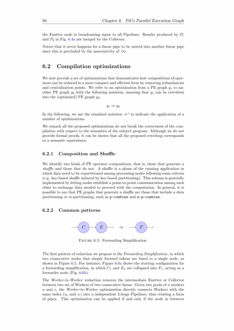
94 Chapter 6. PiCo Parallel Execution Graph
the Emitter node is broadcasting input to all Pipelines. Results produced by P1
and P2 in Fig. 6.4a are merged by the Collector.
Notice that it never happens for a linear pipe to be nested into another linear pipesince this is precluded by the associativity of to.
6.2 Compilation optimizations
We now provide a set of optimizations that demonstrates how compositions of oper-ators can be reduced in a more compact and efficient form by removing redundanciesand centralization points. We refer to an optimization from a PE graph g1 to an-other PE graph g2 with the following notation, meaning that g1 can be rewritteninto the (optimized) PE graph g2:
g1 ⇒ g2
In the following, we use the standard notation ⇒∗ to indicate the application of anumber of optimizations.
We remark all the proposed optimizations do not break the correctness of the com-pilation with respect to the semantics of the subject program. Although we do notprovide formal proofs, it can be shown that all the proposed rewriting correspondsto a semantic equivalence.
6.2.1 Composition and Shuffle
We identify two kinds of PE operator compositions, that is, those that generate ashuffle and those that do not. A shuffle is a phase of the running application inwhich data need to be repartitioned among processing nodes following some criteria(e.g. key-based shuffle induced by key-based partitioning). This schema is generallyimplemented by letting nodes establish a point-to-point communication among eachother to exchange data needed to proceed with the computation. In general, it ispossible to say that PE graphs that generate a shuffle are those that include a datapartitioning or re-partitioning, such as p-combine and w-p-combine.
6.2.2 Common patterns
C E ⇒ F
Figure 6.5: Forwarding Simplification
The first pattern of reduction we propose is the Forwarding Simplification, in whichtwo consecutive nodes that simply forward tokens are fused to a single node, asshown in Figure 6.5. For instance, Figure 6.6a shows the starting configuration fora forwarding simplification, in which C1 and E2 are collapsed into F1, acting as aforwarder node (Fig. 6.6b).
The Worker-to-Worker reduction removes the intermediate Emitter or Collectorbetween two set of Workers of two consecutive farms. Given two pools of n workersu and v, the Worker-to-Worker optimization directly connects Workers with thesame index (ui and vi) into n independent 2-stage Pipelines, thus creating a farmof pipes. This optimization can be applied if and only if the node in between

6.2. Compilation optimizations 95
the two pools is only forwarding data or synchronization tokens. For instance, aWorker-to-Worker optimization is applied in the optimization of Figure 6.6b intoFigure 6.6c.
It is also possible to apply a further optimization to the Worker-to-Worker scenario,that we call Workers Fusion. It consists in fusing two connected workers (as theresult of a Worker-to-Worker optimization) into a single node, thus eliminating anyintermediate communication. However for simplicity we do not show the WorkersFusion in the following sections even where it is applicable.
The All-to-All optimization is valid when a shuffle is required. The starting con-figuration of nodes is the same as for the Worker-to-Worker optimization. Thecentralization point is defined by an emitting node partitioning data following a πpolicy. This centralization can be dropped by connecting all worker nodes with anall-to-all pattern and moving the partitioning logic to each upstream worker ui. Forinstance, this optimization is applied in Figure 6.8. When optimizing Figure 6.8binto Figure 6.8c, the partitioning policy is moved to each map node, that are deputedto send data to the correct destination Worker.
If the Emitter node is also preparing data for windowing (as in Figure 6.10), thisrole has to be moved to the downstream workers. Since each downstream workerreceives data from any upstream peer, some protocol is needed in order to guaranteethe time-ordering is preserved within each partition.

96 Chapter 6. PiCo Parallel Execution Graph
6.2.3 Operators compositions
Following, we show some applications of the optimization patterns defined above.
Composition of map and flatmap
u1 v1
E1 C1 E2 C2
un vn
(a)C Jmap fK ◦ C Jmap gKC Jflatmap fK ◦ C Jflatmap gK
⇓
u1 v1
E1 F1 C2
un vn
(b) Result of Forwarding Simplification optimization
⇓
u1 v1
E1 C2
un vn
(c) Final network resulting from the Worker-to-Worker optimization.
Figure 6.6: Compilation of map-to-map and flatmap-to-flatmap composition.
In Figure 6.6 we describe the compilation of a composition of two consecutive map
or flatmap operators—compiling the to composition of two Pipelines having asmap and flatmap operators that produces the same outcome. In this example, bothWorker-to-Worker and Forwarding Simplification optimizations are applied.

6.2. Compilation optimizations 97
Composition of map and reduce
u1 v1
E1 C1 E2 C2
un vn
(a) C Jmap fK ◦ C Jreduce ⊕K
⇓∗
u1 v1
E1 C2
un vn
(b) Final network resulting from Worker-to-Worker and Forwarding Simplification.
Figure 6.7: Compilation of map-reduce composition.
The optimization of a map-reduce composition, shown in Figure 6.7, is analogousto the map-map case. This is possible since the flat reduce (i.e. neither windowingnor partitioning) poses no requirement on ordering of data items.

98 Chapter 6. PiCo Parallel Execution Graph
Composition of map and p-reduce
u1 v1
E1 C1 p-E2 C2
un vn
(a) C Jmap fK ◦ C Jp-(reduce ⊕) πK
⇓
u1 v1
E1 p-F1 C2
un vn
(b) Result of a Forwarding Simplification optimization
⇓
p-u1 v1
E1 C2
p-un vn
(c) Optimized shuffle by All-to-All optimization
Figure 6.8: Compilation of map-to-p-reduce composition.
Figure 6.8 shows the compilation of a map-to-p-reduce composition. This caseintroduces the concept of shuffle: between the map and p-reduce operators, thedata is said to be shuffled (sometimes referred as parallel-sorted), meaning thatdata is moved from the map workers (i.e., the producers) to the reduce workers(i.e., the consumers) in which data will be reduced by following a partitioningcriteria. By shuffling data, it is possible to assign, to each worker, data belongingto a given partition, and the reduce operator produces a single value for eachpartition. In general, data shuffling produces an all-to-all communication pattern

6.2. Compilation optimizations 99
among map and reduce workers. The all-to-all shuffle is highlighted by the dottedbox in Fig. 6.8c. As an optimization, it is possible to move part of the reducingphase into the map workers, so that each reduce worker computes the final resultfor each key by combining partial results coming from map workers.
Composition of map and w-reduce
u1 w-v1
E1 w-F1 C2
un w-vn
Figure 6.9: Compilation of map-to-w-reduce composition.Centralization in w-F1 for data reordering before w-reduce
workers.
Figure 6.9 shows the compilation of a map-to-w-reduce composition. The first opti-mization step is the same as the one for map-to-w-reduce optimization (Fig. 6.8a),thus this step is not described for simplicity since it shows the forwarding nodesreduction. The centralization point w-F1 is required to reorder items of the streambefore windowing. The final reordering or the reduce value for each window isguaranteed by the C2 Collector.

100 Chapter 6. PiCo Parallel Execution Graph
Composition of map and w-p-reduce
u1 w-v1
E1 w-p-F1 C2
un w-vn
(a) Centralization in w-p-F1 for data reordering before w-p-reduce workers
⇓
p-u1 w-v1
E1 C2
p-un w-vn
(b) Final network resulting from All-to-All simplification, where partitioning is doneby map workers and windowing (for each partition) is done by reduce workers.
Figure 6.10: Compilation of map-to-w-p-reduce composi-tion.
Figure 6.10 shows the compilation of a map-to-w-p-reduce composition. Again weomit the Forwarding Simplification optimization for simplicity. As resulting fromthe first Forwarding Simplification optimization, a centralization point w-p-F1 isneeded to reorder stream items. By applying the All-to-All optimization, it ispossible to make the map operator partition data among downstream nodes. Hencethe reducers reorder incoming data according to time-ordering, apply windowing oneach partition and produce a reduced value for each window.
By comparing the optimized graphs in Figures 6.9 and 6.10, it can be noticed thatadding a partitioning nature to windowed processing enables further optimization.This is not surprising since, as is discussed in [60], the KP pattern is inherentlysimpler than WF. The former can be implemented in such a way that each streamitem is statically mapped to a single Worker, thus reducing both data traffic andcoordination between processing units.

6.3. Stream Processing 101
6.3 Stream Processing
In this section, we discuss some aspects of the proposed execution model from astream processing perspective. In our setting, streams are defined as unboundedordered sequences (cf. Section 5.3.1), thus we consider Dataflow graphs in whichnodes process infinite sequences of tokens.
Historically, all the data-parallel operators we included in the PiCo syntax (e.g.,map, reduce) are defined only for bounded data structures. Although at the syn-tactic level we allow the application of data-parallel operators to streams (e.g., bycomposing an unbounded emit to a map operator), this ambiguity is resolved at thesemantic level, since the semantics of each unbounded operator is defined in termsof its bounded counterpart. For instance, the operators in the combine family aredefined for unbounded collections only if they are endowed with a windowing policy.The semantics of the resulting windowing operator processes each window (i.e., abounded list) by means of the respective bounded semantics (cf. Equation 5.12).
Let us consider the semantic map over streams. As we showed in Section 6.1.1, it isnot possible to implement a strict unbounded semantic map since this would requirereordering all the (infinite) collection at hand. For this reason, we introduced theweak semantic map that can be easily extended to the unbounded case. The resultingsemantics is defined in terms of its bounded counterpart and exploits a batchingmechanism (cf. Equation 5.13).
This approach immediately exposes a trade-off: the width of the batching windows isdirectly proportional to the amount of time-ordering enforced, but it is also directlyproportional to the latency for processing a single item. If a stream is time-ordered(cf. Definition 2), there is no need for reordering, thus the minimum batching (i.e.,width = 1) can be exploited to achieve the lowest latency. Conversely, if the streamis highly time-disordered and we want to restore the ordering as much as possible,we have to pay a price in terms of latency.
We remark that all the frameworks for data processing we consider for compari-son expose similar trade-offs in terms of operational parameters, such as windowtriggering policies [72, 67]. We propose a symmetric approach, in which this as-pect is embedded into the abstract semantics of PiCo programs—rather than theoperational semantics of the underlying runtime.
6.4 Summary
In this Chapter we discussed how a PiCo Pipelines and operators are compiled into adirected acyclic graph representing the parallelization of a given application, namelythe parallel execution dataflow. We showed how each operator is compiled into itscorresponding parallel version, providing a set of optimization applicable when com-posing parallel operators. DAG optimization is present in all analytics frameworkspresented previously in this thesis, and it is done at runtime. Once the applicationis executed, the execution DAG can be optimized by applying some heuristics thatcreate the best execution plan or by applying some pipelining (i.e., in Spark stages)among subsequent operators - thus a strategy similar to optimizations proposedin PiCo. The main strength in PiCo approach is that all proposed optimizationsare statically predefined and they can be provided as pre-built DAG implementeddirectly in the host language. Furthermore, optimizations do not involve operatorsand pipelines only, but it is also specific with respect to the structure type of thePipeline.


103
Chapter 7
PiCo API andImplementation
In this chapter, we provide a comprehensive description of the actual PiCo imple-mentation, both at user API level and at runtime level. We also present a completesource code example (Word Count), which is used to describe how a PiCo programis compiled and executed.
7.1 C++ API
In this section, we present a C++ API for writing programs that can be staticallymapped to PiCo Pipelines, defined in Sect. 5.1. By construction, this approachprovides a C++ framework for data processing applications, each endowed with awell-defined functional semantics (cf. Sect. 5.3) and a clear parallel execution model(cf. Chap. 6).
We opted for a fluent interface, exploiting method cascading (aka. method chaining)to relay the instruction context to a subsequent call. PiCo design exposed in previ-ous chapters makes it independent from the choice of the implementation language.We decided to implement PiCo runtime and API entirely in C++, so that we canexploit explicit memory management, a more efficient runtime in terms of resourcesutilization, and it is possible to take advantage compile time optimizations. Fur-thermore, with C++ it is possible to easily exploit hardware accelerators, makingit more suitable for high-performance applications. Besides this choice can affectportability, we think that the advantages carried by a C++ runtime can overcomethe advantages of having a compile-once-run-everywhere paradigm provided by theJVM. On the other hand, C++ poses some limitations in terms of compatibilitywith well established software for data management used in analytics stacks (Kafka,Flume, Hadoop HDFS), which in some cases provide a limited or no C++ frontend.Consider for instance access to HDFS: besides it exposes a C++ library for read andwrite operations, it is very limited and provides a strongly reduced set of operationswith respect to the Java API.
In the remainder of this section, we provide a full description of all entities in a C++PiCo program, providing also some source code extracts. The current implementa-tion is only for shared memory applications. In the future, an implementation ofthe FastFlow runtime for distributed execution by mean of a Global AsynchronousMemory(GAM) system model. A GAM system consists in a network of executors(i.e., FastFlow workers as well as PiCo operators) accessing a global dynamic mem-ory with weak sharing semantics. With this model, the programming model, thesemantics DAG and its compilation in the parallel execution DAG in PiCo will notchange.

104 Chapter 7. PiCo API and Implementation
7.1.1 Pipe
A C++ PiCo program is a set of operator objects composed into a Pipeline object,processing bounded or unbounded data. A Pipeline can be:
• created as the empty Pipeline, as in the first constructor
• created as a Pipeline consisting of a single operator, as in the second andthird constructors
• modified by adding an operator, as in the add member function
• modified by appending other Pipelines, as in the to member functions
• merged with another Pipeline, as in the merge member function
• paired with another Pipeline by means of a binary operator, as in the pair
member function
Pipe API
Pipe() Create an empty Pipe
template<typename T>
Pipe(const T& op) Create a Pipe from an initial operator
template<typename T>
Pipe(T&& op) Create a Pipe from an initial operator (move)
template<typename T>
Pipe& add(const T& op) Add a new stage to the Pipe
template <typename T>
Pipe& add(T&& op) Add a new stage to the Pipe (move)
Pipe& to(const Pipe& pipe) Append a Pipe to the current one
Pipe& to(std::vector<Pipe*>
pipes)
Append a set of independent Pipes taking inputfrom the current one
template<typename In1,
typename In2, typename Out>Pipe& pair(
const BinaryOperator
<In1, In2> out& a,
const Pipe& pipe)
Pair the current Pipe with a second pipe by a Bi-naryOperator that combines the two input items(a pair) with the function specified by the user
Pipe& merge(const Pipe& pipe) Merge data coming from the current Pipe and theone passed as argument. The resulting collectionis the union of the collection of the two Pipes
void print DAG() Print the DAG as adjacency list and by a BFSvisit
void run() Execute the Pipe
void to dotfile(std::string
filename)
Encode the DAG into a dot file
void pipe time() Return the execution time in milliseconds
Table 7.1: the Pipe class API.
Table 7.1 summarizes the Pipeline class API.

7.1. C++ API 105
In addition to the member functions for creating, modifying and combining Pipelineobjects, the last four member functions may only be called on executable Pipelines,namely those representing top-level PiCo Pipelines (cf. Definition 1). For a Pipelineobject, to be executable is a property that can be inferred from its type. We discussthe typing of Pipeline objects in Sect. 7.1.3.
7.1.2 Operators
The second part of the C++ PiCo API represents the PiCo operators. By followingthe grammar in Sect. 5.1.2, we organize the API in a hierarchical structure ofunary and binary operator classes. The design of the operators API is based oninheritance in order to follow in an easy way the grammar describing all operators,nevertheless we recognize that the use of template programming without inheritancewould improve runtime performance. The implementation makes use of dynamicpolymorphism when building the semantics DAG, where virtual member functionsare invoked to determine the kind of operator currently processed.
UnaryOperator is the base class representing PiCo unary operators, those with nomore than one input and/or output collection. For instance, a Map object takesa C++ callable value (i.e., the kernel) as parameter and represents a PiCo oper-ator map, which processes a collection by applying the kernel to each item. AlsoReadFromFile is a sub-class of UnaryOperator and it represents those PiCo op-erators that produce a (bounded) unordered collection of text lines, read from aninput file.
BinaryOperator is the base class representing operators with two input collectionsand one output collection. For instance a BinaryMap object represents a PiCooperator b-map, that processes pairs of elements coming from two different inputcollections and produces a single output for each pair. A BinaryMap object ispassed as parameter to Pipeline objects built by calling the pair member function(cf. Table 7.1).

106 Chapter 7. PiCo API and Implementation
Operator Constructors
template<typename In, typename Out>
Map(std::function<Out(In&)> mapf)Map constructor by defining its ker-nel function mapf : In→ Out
template<typename In, typename Out>
FlatMap(std::function<void(In&,
FlatMapCollector<Out>& flatmapf)
FlatMap constructor by defin-ing its kernel function flatmapf :〈In, F latMapCollector〈Out〉 〉 →void
template<typename In>
Reduce(std::function<In(In&, In&)>
reducef)
Reduce constructor by defin-ing its kernel function reducef :〈In, In〉 → In
template<typename In>
PReduce(std::function<In(In&, In&)>
preducef)
PReduce constructor by defin-ing its kernel function preducef :〈In, In〉 → In on partitioned in-put (i.e., reduce by key)
template<typename In1, typename In2>
BinaryMap(std::function<Out(In1&, In2&)>
bmapf)
BinaryMap constructor by defin-ing its kernel function bmapf :〈In1, In2〉 → Out
ReadFromFile()ReadFromFile constructor to readinput data from file, each line is re-turned to the user as std::string
template<typename Out>
ReadFromSocket(char delimiter)ReadFromSocket constructor toread input data from Socket, linesare separated by a user-defined de-limiter and returned to the user asstd::string
template<typename In>
WriteToDisk(std::function<std::string(In&)>
func)
WriteToDisk constructor to writeto the specified textfile by definingits kernel function: In→ void
template<typename In>
WriteToStdOut(std::function<std::string(In&)>
func)
WriteToStdOut constructor towrite to the standard outputby defining its kernel function:In→ void
Table 7.2: Operator constructors.
Table 7.2 summarizes the constructors of C++ PiCo operators. In the followingsections, we describe all the implemented classes, showing also their inheritanceclass diagrams.
The map family
Map is a UnaryOperator. As we anticipated above, it represents the PiCo operatormap, which process an input collection by applying a user-defined kernel (a C++callable value) to each item.
Similarly, FlatMap represents the flatmap operator, which produces zero, one ormore elements upon processing each item from the input collection. A FlatMap
object takes as input a FlatMapCollector object, representing the storage for theitems produced by each execution of the kernel. An example of the resulting inter-face is reported in Listing 7.1.

7.1. C++ API 107
Operator
UnaryOperator<In, Out>
FlatMap<In,Collector<Out>> Map<In, Out>
Figure 7.1: Inheritance class diagram for map and flatmap.
Operator
UnaryOperator<In, In>
Reduce<In> PReduce<In>
Figure 7.2: Inheritance class diagram for reduce andp-reduce.
In case of ordered collections, we opted for implementing the above classes in theirweak semantic version (defined in Sect. 5.3.2, Eq. 5.13 for map operator) for bothbounded and unbounded processing. This allows to design a simpler and moreefficient runtime, as we will discuss later.
Fig. 7.1 reports the inheritance class diagram for Map and FlatMap classes.
The combine family
Reduce is the UnaryOperator representing the PiCo operator reduce. It synthesizesall the elements in the input collection into an atomic value, according to a user-defined binary kernel (a C++ callable value).
PReduce represents the PiCo operator p-reduce, thus it produces one synthesizedvalue for each partition extracted from the input collection by the partitioningpolicy.
Fig. 7.2 reports the inheritance class diagram for Reduce and PReduce classes.
A windowing policy can be added to Reduce and PReduce objects by invoking thewindow member function. A windowing Reduce (or PReduce) logically splits theinput collections into windows, according to the user-provided policy, and producesone synthesized value for each window.
Since we only provide a prototypical implementation, we only support the commonby-key partitioning policy, thus only supporting reduction of key-value collections.Moreover, we only provide count-based tumbling windows.
Listing 7.1 illustrates a Pipeline using the partitioning and windowing variant ofReduce. In the example, the windowing policy is tumbling and count-based withwidth 8.

108 Chapter 7. PiCo API and Implementation
1 // define batch windowing
2 size_t size = 8;
3
4 // define a generic word-count pipeline
5 Pipe countWords;
6 countWords
7 .add(FlatMap<std::string, std::string>(tokenizer))
8 .add(Map<std::string, KV>([&](std::string in)
9 {return KV(in,1);}))
10 .add(PReduce<KV>([&](KV v1, KV v2)
11 {return v1+v2;}).window(size));
Listing 7.1: creating a simple Pipeline in the C++PiCo API.
Sources and Sinks
As we will discuss in Sect. 7.1.3, source and sink objects play the crucial role ofspecifying the type of the collections processed by the Pipeline they belong to.
ReadFromFile and ReadFromSocket are sub-classes of InputOperator, a class rep-resenting PiCo sources, that produce the collections to be processed by the down-stream Pipeline objects. The data populating the collections is read from either atext file, as for ReadFromFile, or a TCP/IP socket, as for ReadFromSocket.
Operator
UnaryOperator<void, Out>
InputOperator<Out>
ReadFromFile<Out> ReadFromSocket<Out>
Figure 7.3: Inheritance class diagram for ReadFromFile
and ReadFromSocket.
Figure 7.3 reports the inheritance class diagram for the InputOperator classes.
WriteToDisk and WriteToStdOut are sub-classes of OutputOperator, a class rep-resenting PiCo sinks, which consume the collections produced by the upstreamPipeline objects. The data is written to either a text file, as for WriteToDisk, orthe standard output, as for WriteToStdOut. Moreover, a user-defined kernel (aC++ callable value) is used to process the data prior to writing them to the properdestination.

7.1. C++ API 109
Operator
UnaryOperator<In, void>
OutputOperator<In>
WriteToDisk<In> WriteToStdOut<In>
Figure 7.4: Inheritance class diagram for WriteToDisk andWriteToStdOut.
Figure 7.4 reports the inheritance class diagram for the OutputOperator classes.
Input file, output file, server name and port are passed to the application as argu-ments of the executable: -i and -o for the input and output file respectively, -s todefine server address and -p to define the listening port.
We remark the presented API is a prototypical implementation, therefore a limitedset of source and sink objects are provided only for exemplification.
7.1.3 Polymorphism
One distinguishing feature of the PiCo programming model, differently from state-of-the-art frameworks, is that the same syntactic object (e.g., a Pipeline or anoperator) can be used to process data collections having different types. For exam-ple, the word-count Pipeline in Algorithm 1 can be used to process bags, streamsand lists once combined with proper sources and sinks. This feature is enabledby the type system we defined in Sect. 5.2 that allows polymorphic Pipelines andoperators. More precisely, Pipelines and operators are polymorphic with respect toboth the data type (the type of the collection items) and the structure type (the“shape” of the collection, such as bag or stream).
In the proposed C++ API, the data type polymorphism is expressed at compile-time by implementing operators as template classes. As reported in Table 7.2, eachoperator takes a template parameter representing the data type of the collectionsprocessed by the operator. Moreover, each Pipeline object is decorated by the setof the supported structure type s.
We recall that all the polymorphism is dropped in top-level Pipelines. Therefore,executable Pipeline objects have an unique type. By construction, InputOperatorsplay the important role of specifying the unique structure type processed by the ex-ecutable Pipeline they belong to. For instance, a Pipeline starting with an operatorof ReadFromFile type will only process multi-sets, whereas a Pipeline starting withan operator of ReadFromSocket type will only process streams.
In the following paragraphs we provide some insight about the type checking andinference processes, which are an implementation of the type system discussed inSect. 5.2.
Although Pipeline types are not fully exposed by the C++ API, they are exploitedby the runtime to ensure only legal PiCo Pipelines are built, thus they are part ofthe API specification.
When a member function is called on a Pipeline object, the runtime performs thetwo following actions on the subject Pipeline:

110 Chapter 7. PiCo API and Implementation
1. it checks the legality of the call by inspecting the type of both the subjectPipeline and the call arguments (type checking)
2. it updates the type of the subject Pipeline (type inference)
We recall that each PiCo Pipeline has an input and output cardinality, either 0 or1. For instance, top-level Pipelines have both input and output cardinality equalto zero. We say a Pipeline with non-zero input cardinality is a consumer since itconsumes a collection, thus it needs to be prefixed by a source operator in orderto be executed. Similarly, we say a Pipeline with non-zero output cardinality is aproducer. For instance, the simple Pipe in Listing 7.1 is a producer.
When calling a member function on a Pipeline p object causing the addition of anoperator a (i.e., add or pair), the invocation fails if any of the following conditionsholds (i.e. type checking fails):
1. p is neither empty nor a producer, that is, it has already a sink operator (e.g.,a WriteToDisk)
2. data type compatibility check fails, for instance because the output data typeof p (i.e., the output data type of p’s last operator) differs from the the inputdata type of a
3. structure type s are incompatible, for instance a is a windowing operator andp only processes bags
Furthermore, after adding the operator a, the type of p is updated as follows:
1. p takes the a’s input or output degree if a is an input or output operator
2. the new p’s structure type is defined as the intersection of the structure types of p and a
When modifying p by appending another Pipeline q, the to member function failsif any of the following conditions holds:
1. p is neither empty nor a producer
2. p is not empty and q is not a consumer
3. data type or structure type compatibility check fails
When appending multiple Pipelines (resulting into a branching Pipeline), the pre-vious constraints are still checked for each Pipeline to be added.
In case of merging or pairing, in addition to the above conditions, it is also checkedthat at least one of the two Pipelines to be combined is a non-producer one. Thisway it is guaranteed that any Pipeline has 0 or 1 entry and exit points and thereforeit can be attached to other Pipelines and operators.

7.2. Runtime Implementation 111
7.1.4 Running Example: Word Count in C++ PiCo
Listing 7.2 shows a complete example of the Word Count benchmark.
1 typedef KeyValue<std::string, int> KV;
2
3 static auto tokenizer = [](std::string& in,FlatMapCollector<KV>& collector) {
4 std::istringstream f(in);
5 std::string s;
6 while (std::getline(f, s, ’ ’)) {
7 collector.add(KV(s,1));
8 }
9 };
10
11 int main(int argc, char** argv) {
12 // parse command line
13 parse_PiCo_args(argc, argv);
14
15 /* define a generic word-count pipeline */
16 Pipe countWords;
17 countWords
18 .add(FlatMap<std::string, std::string>(tokenizer)) //
19 .add(Map<std::string, KV>([&](std::string in)
20 {return KV(in,1);}))
21 .add(PReduce<KV>([&](KV v1, KV v2)
22 {return v1+v2;}));
23
24 /* define i/o operators from/to file */
25 ReadFromFile reader();
26 WriteToDisk<KV> writer([&](KV in) {
27 return in.to_string();
28 });
29
30 /* compose the pipeline */
31 Pipe p2;
32 p2 //the empty pipeline
33 .add(reader) // add single operator
34 .to(countWords) // append a pipeline
35 .add(writer); // add single operator
36
37 /* execute the pipeline */
38 p2.run();
39
40 return 0;
41 }
Listing 7.2: Word Count example in PiCo.
7.2 Runtime Implementation
The runtime of PiCo is implemented on top of the FastFlow library, so that weuse ff node, ff pipeline and ff farm as building blocks for the representa-tion of the parallel execution graph (as described in Chap. 6). In this section, wedescribe how each component of PiCo is effectively mapped to a FastFlow nodeor pattern. We recall that by exploiting the FastFlow runtime, it is possible tomove only pointers to data among ff nodes, using these pointers as capabilitiesfor synchronizations (see Sect. 2.4.1).
Pipe The Pipe class in the user API represents the main entity in a PiCo ap-plication. When the run() member function is invoked on a Pipe, the emptyff pipeline corresponding to the Pipe is created. After that, the semanticsDAG (Sect. 5) representing the application is visited and, recursively, ff farmsand ff nodes are added as stages to the ff pipeline, depending on the currentvisited node. We recall that, in FastFlow, each ff node is a thread.

112 Chapter 7. PiCo API and Implementation
Map, Flatmap, Reduce and PReduce operators are implemented asff farms. A parallelism parameter defines how many workers are created in eachfarm. The total number of threads per ff farm is one for the Emitter node, onefor the Collector node and parallelism number of threads for workers. Worker nodesexecute the kernel code specified at API level on each item received. The Collectornode receives data from workers in a from-any policy and forwards them to the nextstage of the Pipe.
A different implementation for Emitter and Collector is provided for the p-reduce
farm. In this case, the Emitter node has to take care of partitioning items on theirgroup basis (i.e., by key). More precisely, the Emitter partitions the key spaceamong workers, forwarding elements belonging to the same group always to thesame worker (of course, it is possible for one worker to receive more than one keyto process). The Collector will start gathering results only when workers are donewith partitioned reduce.
Input and output operators are implemented as single ff nodes. These nodeshave specialized code performing input and output operations. Moreover, inputnodes are instructed to send an End Of Stream (EOS) when the input generationcompletes. The EOS is implemented into two distinct tokens: the FF EOS isinternal to the FastFlow runtime and it instructs ff nodes to terminate after itsreception. The PICO EOS is internal to PiCo and processed by all ff nodes,and it does not cause the termination of ff nodes. It is used, for instance, by thep-reduce Emitter node to instruct workers that the end of stream/file is reachedand to forward their reduce results to the Collector before terminating with theFF EOS.
To and Merge are Pipe member functions for appending and merging pipes,respectively. In this paragraph, we consider the merge member function having sig-nature Pipe& merge(const Pipe& pipe). The merging invocation results in theinstantiation of a ff farm where the two Pipes to be merged are added as a work-ers as new ff pipelines—this is possible thanks to the FastFlow composabilityproperty (see Sect. 2.4.1).
Figure 7.5 shows an example of the DAG resulting from merging three pipelines.EntryPointMERGE is the ff farm Emitter node, while the Merge node is its Col-lector receiving all results to be forwarded to subsequent stages (in this case, awrite-to-disk ff node writing to void.txt file). The EntryPointMERGE broad-casts a PICO SYNC token to the Pipes to be merged in order to start generatinginput items (read from nopunct.txt file). Further information about the PICO -SYNC token are reported in Section 7.3.4. We recall that the order of items isrespected only locally to each Pipe, while there exists an interleaving order in theoutput from the Collector.
Figure 7.5: Semantics DAG resulting from merging threePipes.

7.3. Anatomy of a PiCo Application 113
We recall that the order of items is respected only locally to each Pipe, while thereexists a certain interleaving order in output from the Collector. When mergingpipelines, the Emitter is always the first stage of the PiCo pipeline.
7.3 Anatomy of a PiCo Application
In this section, we provide a description of the PiCo execution model. For the sakeof simplicity and completeness, we start from the source code of a PiCo applicationand we explain each step taken to reach the result.
7.3.1 User level
As a concrete example, shown in Listing 7.3, we use an application in which twoPipes are merged. These two Pipes take as input data from two files and map eachline into a <string, int> pair. Then, each pair is written to a file.
1 typedef KeyValue<std::string, int> KV;
2 parse_PiCo_args(argc, argv);
3 /* define the operators */
4
5 auto map1=Map<std::string, KV>([](std::string in)
6 {return KV(in, 1);});
7
8 auto map2=Map<std::string, KV>([](std::string in)
9 {return KV(in, 2);});
10
11 auto reader=ReadFromFile<std::string>();
12
13 auto wtd=WriteToDisk<KV>([](KV in) {
14 std::string value = "<";
15 value.append(in.Key())
16 .append(", ")
17 .append(std::to_string(in.Value()))
18 .append(">");
19 return value;
20 });
21
22 /* p1 read from file and process it by map1 */
23 Pipe p1(reader);
24 p1.add(map1);
25
26 /* p2 read from file and process it by map2 */
27 Pipe p2(reader);
28 p2.add(map2);
29
30 /* now merge p1 with p2 and write to file */
31 p1.merge(p2);
32 p1.add(wtd);
33
34 /* execute the pipeline */
35 p1.run();
Listing 7.3: Merging example in PiCo.
The input reader operator reads lines from a text file and simply returns each lineread unmodified. Since data is read from disk, the structure type determined bythe input operator is a bag (bounded, unordered). The output wtd operator takesall pairs of the type KeyValue KV and processes them with the user defined lambdaexpression.
Operators map1 and map2 take as input a line from their reader operator and pro-duce a KeyValue KV pair: the input line is the key and the C++ lambda auto

114 Chapter 7. PiCo API and Implementation
map1 = Map<std::string, KV>([](std::string in){return KV(in, 1)}) pro-duces key-value pairs having input lines as key and value 1 as value, whereas map2
gives value 2 to each pair. A copy of reader is used to compose the second pipePipe p2(reader), which is then merged to the p1 by p1.merge(p2). We recallthat compatibility check on structure type and the type check on last output typeand new operator’s input type is performed if the Pipe is not empty (Sect. 7.1.1).
7.3.2 Semantics dataflow
While composing the Pipe, the semantics dataflow graph is also created, that is, thedataflow representing the semantics of the (sequential) application in the form of adirected acyclic graph (see Chapter 4), where vertexes represent operators and edgesrepresent data dependencies. This step is done while calling Pipe modifiers, thusno further Pipe preprocessing is needed to build the semantics DAG, representedas an adjacency list and implemented by a std::map. It is possible to visualize theDAG by invoking the to dotfile() member function on the Pipe. The resultingDAG of the example application is shown in Figure 7.3.
Figure 7.6: Semantics DAG resulting from the applicationin listing 7.3.
The class representing each node holds the information about its role in the seman-tics DAG. The role determines if the node is a processing node (i.e., an operator) oran auxiliary node that does not process data (i.e., the EntryPointMERGE node).
The role can have three different values: 1) Processing, representing an operatorwith user-defined code; 2) EntryPoint/ExitPoint, as the EntryPointMERGE andMerge nodes in Fig. 7.6 when merging Pipes (as well as Merge node in Fig. 7.7);3) BCast node representing the starting point resulting from the invocation of theto(std::vector<Pipe*> pipes) member function as shown in Figure 7.7.
Figure 7.7: Semantics DAG resulting from connecting mul-tiple Pipes.
7.3.3 Parallel execution dataflow
When the run() member function is called on p1, the semantics dataflow is pro-cessed to create the parallel execution dataflow. This graph represents the applica-tion in terms of processing elements (i.e., actors) connected by data channels (i.e.,edges), where operators can be replicated to express data parallelism. This can bean intermediate representation of the possible parallelism exploitation, as shown inSect. 6.1, where we provided the compilation of each operator in terms of patterns(e.g., farm). We implemented this intermediate representation directly in FastFlowby using nodes, farms and pipelines patterns.
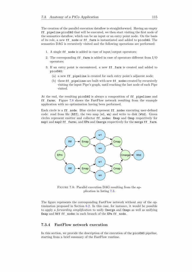
7.3. Anatomy of a PiCo Application 115
The creation of the parallel execution dataflow is straightforward. Having an emptyff pipeline picoDAG that will be executed, we then start visiting the first node ofthe semantics dataflow, which can be an input or an entry point node. On the basisof its role, a new ff node or ff farm is instantiated and added to picoDAG. Thesemantics DAG is recursively visited and the following operations are performed:
1. A single ff node is added in case of input/output operators;
2. The corresponding ff farm is added in case of operators different from I/Ooperators;
3. If an entry point is encountered, a new ff farm is created and added topicoDAG;
(a) a new ff pipeline is created for each entry point’s adjacent node;
(b) these ff pipelines are built with new ff nodes created by recursivelyvisiting the input Pipe’s graph, until reaching the last node of each Pipevisited.
At the end, the resulting picoDAG is always a composition of ff pipelines andff farms. Figure 7.8 shows the FastFlow network resulting from the exampleapplication with no optimization having been performed.
Each circle is a ff node. Blue circles represent ff nodes executing user-definedcode: read from file (Rff), the two map (w1, wn) and write to disk (Wtd). Greencircles represent emitter and collector ff nodes: Emap and Cmap respectively formap1 and map2 ff farms, and EPm and Cmerge respectively for the merge ff farm.
EPm
Rff
Rff
w1
wn
Emap
Emap
w1
wn
Cmap
Cmap
Cmerge Wtd
Figure 7.8: Parallel execution DAG resulting from the ap-plication in listing 7.3.
The figure represents the corresponding FastFlow network without any of the op-timization proposed in Section 6.2. In this case, for instance, it would be possibleto apply a forwarding simplification to unify Cmerge and Cmaps as well as unifyingEmap and Rff ff nodes in each branch of the EPm ff node.
7.3.4 FastFlow network execution
In this section, we provide the description of the execution of the picoDAG pipeline,starting from a brief summary of the FastFlow runtime.

116 Chapter 7. PiCo API and Implementation
From the orchestration viewpoint, the process model to be employed is a Communi-cating Sequential Processes CSP1/Actor hybrid model where processes (ff nodes)are named and the data paths between processes are explicitly identified (differentlyfrom the Actor model). The abstract units of communication and synchronizationare known as channels and represent a stream of data exchanged between two pro-cesses. Each ff node is a C++ class entering an infinite loop through its svc()
member function where:
1. it gets a task from input channel (i.e., a pointer);
2. it executes business code on the task;
3. it puts a task into the output channel (i.e., a pointer)
Representing communication and synchronization by a channel ensures that syn-chronization is tied to communication and allows layers of abstraction at higherlevels to compose parallel programs where synchronization is implicit. For a morecomplete review of FastFlow, please refer to Section 2.4.1.
Patterns to build a graph of ff nodes, such as farms, are defined in the core patternslevel of FastFlow stack reported in Figure 2.8. Since the graph of ff nodes is astreaming network, any FastFlow graph is built using two streaming patterns (farmand pipeline) and one pattern-modifier (loopback, to build cyclic networks). Thesepatterns can be nested to build arbitrarily large and complex graphs. Each ff node
in a ff pipeline or ff farm corresponds to a thread.
In a PiCo application, as the one in Fig. 7.8, a compiled DAG can start with aninput node or with an entry point obtained by the compilation of a merge operator.In the case of an entry point (such as the first stage of the ff pipeline in theexample), this node is instructed to send to all its neighbor nodes a token (specificto the PiCo runtime, called PICO SYNC ), using a round-robin policy.
This token makes the computation start on input nodes Rff shown in Figure 7.8.When the input tokens generation ends, the ff node corresponding to the Rff
operator sends a PICO EOS token and exits from the svc() member function2.On exit, it terminates its life-cycle by emitting the FastFlow FF EOS token. Dif-ferently from all other operators ff nodes, which are executed as many times asthe number of input data they process (i.e., on a stream of microbatches), an inputnode’s svc() is executed only once and stops on input termination.
In the running example, both Rff nodes read lines from a file that are then forwardedto their following node of the pipeline. Tokens are sent out at microbatch granularity(in this case, a microbatch is a fixed size array of lines read from the input file).
Following our example, the next stages of both Rffs are the Emitters of the map
farms. Since we implemented PiCo’s parallel operators following the weak seman-tic map (defined in Sect. 5.3.2, eq. 5.13 for map operator) on both bounded orunbounded processing, the map ff farms process microbatches instead of singletokens.
Each worker of the map ff farm processes the received microbatch by applyingthe user-defined function. Then each worker allocates a new microbatch to storethe result of the user-defined function, and then deleting the received microbatch.The new microbatch is forwarded to the next node. The general behavior of aworker during its svc() call is that it deletes each input microbatch (allocatedby the Emitter) after it has been processed and the results of the kernel function(applied to all elements of the microbatch) are stored into a new microbatch. When
1The CSP model describes a systems in terms of component processes operating inde-pendently, which interact with each other through message-passing communication.
2We recall that the svc() member function of a ff node executes the kernel code ofthe operator.

7.4. Summary 117
received, PICO EOS or PICO SYNC tokens are forwarded as well. When theCollector receives PICO EOS tokens from all workers, it then forwards the PiCoend of stream token to the next stage, namely the Cmerge node.
The Cmerge ff node implements a from-any policy to collect results. Then itforwards results to the next stage, in this case the output operator Wtd. This lastnode is a single sequential ff node (we recall that input and output processingnodes are always sequential), writing the received data to a specified file. WhenWtd receives PICO EOS, the file is closed and the computation terminates.
At this point, the FastFlow runtime manages ff nodes destruction and runtimecleanup.
7.4 Summary
In this Chapter we provided a description of the actual PiCo implementation, bothat user API level and at runtime level. PiCo API implementation follows a fluentinterface, exploiting method cascading (aka. method chaining) to relay the instruc-tion context to a subsequent call. It is implemented entirely in C++, so that we canexploit explicit memory management, a more efficient runtime in terms of resourcesutilization, and it is possible to take advantage compile time optimizations. Thedesign of the operators API is based on inheritance in order to follow in an easyway the grammar describing all operators, nevertheless we recognize that the useof template programming without inheritance would improve runtime performance.The implementation makes use of dynamic polymorphism when building the se-mantics DAG, where virtual member functions are invoked to determine the kindof operator currently processed.
We described the anatomy of PiCo runtime starting from a complete source codeexample (Word Count). The Pipeline described in the source code is first providedas the semantics DAG, then we went through the compilation step, in which thePipeline is compiled into the parallel execution graph (namely, the parallel exe-cution DAG). The parallel execution graph, which is agnostic with respect to theimplementation, is converted to a FastFlow network of patterns that results fromthe composition of ff pipeline and ff farms. Finally, the effective executionis described, which is available in shared memory only. In the future, an imple-mentation of the FastFlow runtime for distributed execution by mean of a GlobalAsynchronous Memory(GAM) system model. A GAM system consists in a networkof executors (i.e., FastFlow workers as well as PiCo operators) accessing a globaldynamic memory with weak sharing semantics.


119
Chapter 8
Case Studies andExperiments
This chapter provides a set of experiments based on examples defined in Sect. 5.4.We compare PiCo to Flink and Spark, focusing on expressiveness of the program-ming model and on performances in shared memory.
8.1 Use Cases
We tested PiCo with both batch and stream applications. A first set of experimentscomprehends the word count and stock market analysis. We now describe each usecase, also providing source code snapshots reporting classes related to the core ofeach application. All listings are reported in Appendix A.
8.1.1 Word Count
Considered as the “Hello, World!” of Big Data analytics, a word count applicationtypically belongs to batch processing.
The input is a text file, which is split into lines. Then, each line is tokenized intowords: this operation is implemented as a flatmap, which outputs a number ofitems depending on the input line. Each of these items, namely the words of theinput file, are processed by a map operator which produces a key-value pair < w, 1 >for each word w. After each word has been processed, all pairs are grouped by thevalues of each pair are reduced by a sum. The final result is a single pair for eachword, where the value represents the number of occurrences of a word in the text.
A PiCo word count application can be found in listing 7.2.
The source code for Flink and Spark Word Count are shown in listings A.3 and A.6respectively.
8.1.2 Stock Market
The following examples implements the use cases reported in Sect. 5.4. The first usecase implements the “Stock Pricing” program that computes a price for each optionread from a text file. Each line is parsed to extract stock names followed by stockoption data. A map operator then computes prices by means of the Black & Scholesalgorithm for each option and, finally, a reducer extracts the maximum price foreach stock name. In the following sections, we provide source codes extracts forimplementation in PiCo (listing A.1), Flink (listing A.4) and Spark (listing A.7).

120 Chapter 8. Case Studies and Experiments
8.2 Experiments
The architecture used for experiments is the Occam Supercomputer (Open Com-puting Cluster for Advanced data Manipulation) [127, 8], designed and managedby the University of Torino and the National Institute for Nuclear Physics.
Occam has the following technical characteristics:
• 2 Management Nodes: CPU - 2x Intel R© XeonR© Processor E5-2640 v38 core 2.6GHz, RAM - 64GB/2133MHz, Disk - 2x HDD 1Tb Raid0, Net -IB 56Gb + 2x10Gb + 4x1GB, FormFactor - 1U
• 4 Fat Nodes: CPU - 4x IntelR© XeonR© Processor E7-4830 v3 12 core/2.1Ghz,RAM - 768GB/1666MHz (48 x 16Gb) DDR4, Disk - 1 SSD 800GB + 1 HDD2TB 7200rpm, Net - IB 56Gb + 2x10Gb
• 32 Light Nodes: CPU - 2x IntelR© XeonR© Processor E5-2680 v3, 12 core2.5Ghz, RAM - 128GB/2133 (8x16 Gb), Disk - SSD 400GB SATA 1.8 inch,Net - IB 56Gb + 2x10Gb, FormFactor - high density (4 nodes x RU)
• 4 GPU Nodes: CPU - 2x IntelR© XeonR© Processor E5-2680 v3, 12 core2.1Ghz, RAM - 128GB/2133 (8x16Gb) DDR4, Disk - 1 x SSD 800GB sas 6Gbps 2.5 inch, Net - IB 56Gb + 2x10Gb, GPU - 2 x NVIDIA K40 on PCI-EGen3 x16
• Scratch Disk: Disk - HDD 4 TB SAS 7200 rpm, Capacity - 320 TB RAW+ 256 TB usable, Net - 2 x IB 56Gb FDR + 2 x 10Gb, File System - LustreParallel Filesystem
• Storage: Disk - 180 x 6 TB 7200 rpm SAS 6Gbps, Capacity - 1080 TB raw768 TB usable, Net - 2 x IB 56Gb + 4 x 10GbE, File System - NFS export,Fault Tolerance - RAID 6 Equivalent with Dynamic Disk Pools
• Network: IB layer - 56 Gbps, ETH10G layer - 10 Gbps, IB topology -FAT-TREE, ETH10G topology - FLAT
We performed tests on scalability and best execution time comparing PiCo to Sparkand Flink on batch and stream applications. The current experimentation is only onshared memory applications. In the future, an implementation of the FastFlow run-time for distributed execution by mean of a Global Asynchronous Memory(GAM)system model1, so that we will be able to have a performance evaluation also in adistributed memory model.
8.2.1 Batch Applications
In the first set of experiments, we run the Word Count and Stock Pricing examplesreported in the previous section. First, we show scalability obtained by PiCo withrespect to the number of parallel threads used for parallel operators.
We compute the scalability factor as the relation between the execution time withparallelism 1 (i.e., sequential operators) and the execution time obtained by exploit-ing more parallelism. It is defined as T1/Ti ∀ i ∈ {1, . . . , nc} with nc representingthe number physical cores of the machine. The maximum number of physical coresis 48 on Fat Nodes (4 x IntelR© XeonR© Processor E7-4830 v3 12 core/2.1Ghz).
1A GAM system consists in a network of executors (i.e., FastFlow workers as well asPiCo operators) accessing a global dynamic memory with weak sharing semantics.

8.2. Experiments 121
PiCo
By default, PiCo allocates a single worker thread in each farm corresponding toan operator, and allocates microbatches with size 8 to collect computed data (seeSect. 6.1.1 for batch semantics). We tested PiCo with different microbatch sizesto measure its scalability also with respect to number of microbatches allocations.The best size for microbatch is 512 elements, which naturally leads to a reductionof dynamic memory allocations.
To increase performance, we also used two different threads pinning strategy. Thedefault pinning strategy in Occam is interleaved on physical cores first, so that eachconsecutive operator of the pipeline is mapped to a different socket of the node. Inthis scenario, a linear mapping using physical cores first helped in reducing memoryaccess time to data, since allocations are done mainly in the memory near the threadthat is accessing that data.
Figure 8.1 shows scalability and execution times for the Word Count application:each value represents the average of 20 runs for each number of workers, the micro-batch size is 512, and the thread pinning strategy is physical cores first. The sizeof the input file is 600MB. It a text file of random words taken from a dictionary of1K words. In the Word Count pipeline, PiCo instantiates a total of 5 fixed threads(corresponding to sequential operators), plus the main thread, plus a user-definednumber of workers for the flatmap operator. To exploit at most 48 physical cores,we can run at most 42 worker threads.
0
5
10
15
20
25
1 2 4 8 12 16 32 42 48 0
5
10
15
20
25
Exe
cu
tio
n T
ime
(s)
Sca
lab
ility
Fa
cto
r
Parallelism
Pico Scalability and Execution Time on WordCount
Scalability FactorTime (s)
Figure 8.1: Scalability and execution times for Word Countapplication in PiCo.
With 16 and 32 workers for the map operator, mapped on physical cores, PiCoobtains similar average execution times: the best average execution time obtainedis 1.61 seconds with 16 workers and a scalability factor of 13.60.
Figure 8.2 shows scalability and execution times for the Stock Pricing application:each value represents the average of 20 runs for each number of workers, the micro-batch size is 512, and the thread pinning strategy is linear on physical cores first. In

122 Chapter 8. Case Studies and Experiments
the Stock Pricing pipeline, PiCo instantiates a total of 4 fixed threads (correspond-ing to sequential operators), plus the main thread, plus a user-defined number ofworkers for the map +p-reduce operator.
0
5
10
15
20
25
1 2 4 8 12 16 32 42 48 0
5
10
15
20
25
Exe
cu
tio
n T
ime
(s)
Sca
lab
ility
Fa
cto
r
Parallelism
Pico Scalability and Execution Time on StockPricing
Scalability FactorTime (s)
Figure 8.2: Scalability and execution times for Stock Pric-ing application in PiCo.
With 8 workers for the map + p-reduce operator, mapped on physical cores, PiCoobtains the best average execution time of 3.26 seconds and a scalability factorof 6.68.
Limitations on scalability. The applications tested in PiCo showed a com-mon behavior on the first node of each Pipeline—the Read From File (RFF) op-erator. As the number of workers increases, it increases also the execution time ofthe read from file, making it the application’s bottleneck. The RFF’s kernel codeis the following: each line of the input file is read in a std::string and stored intoa fixed-size microbatch. Once the microbatch is full, it is forwarded to the nextoperator and a new microbatch is allocated. This is repeated until the end of file isreached. As the microbatch size increases, the number of their allocation decreasesbut RFF still represents the bottleneck. In tables 8.2 and 8.1, we report executiontimes of a single run of Word Count and Stock Pricing with two different microbatchsizes (8 and 512), showing how the scalability on workers is still increasing despitethe bottleneck on RFF, giving room for improvement on the total execution time.

8.2. Experiments 123
Microbatch size 8 (execution time in ms)
workers exec. time read from file worker worker scalability1 21874.50 901.98 21685.10 1.002 10807.80 915.61 10786.20 2.018 2916.80 1016.87 2753.39 7.87
16 1718.20 1711.02 1535.38 14.1232 1755.85 1743.04 924.14 23.46
Microbatch size 512 (execution time in ms)
workers exec. time read from file worker worker scalability1 22091.60 869.07 22087.20 1.002 11030.70 861.86 11026.50 2.008 2841.45 932.27 2799.31 7.89
16 1635.55 1595.28 1607.74 13.7432 1603.78 1589.13 917.44 24.07
Table 8.1: Decomposition of execution times and scalabil-ity highlighting the bottleneck on ReadFromFile operator in
the Word Count benchmark.
Microbatch size 8 (execution time in ms)
workers exec. time read from file worker worker scalability1 22286.70 2391.62 22048.00 1.002 11549.10 2524.72 11430.20 1.938 3588.49 3586.57 3131.49 7.04
16 5135.71 5133.08 1730.37 12.7432 6096.26 6092.02 934.54 23.59
Microbatch size 512 (execution time in ms)
workers exec. time read from file worker worker scalability1 21775.10 2123.27 21766.70 12 11289.20 2201.70 10946.40 1.998 3328.80 3326.84 2967.67 7.33
16 3370.84 3768.64 2510.13 8.6732 4707.89 4704.69 868.11 25.07
Table 8.2: Decomposition of execution times and scalabil-ity highlighting the bottleneck on ReadFromFile operator in
the Stock Pricing benchmark.
Tables 8.1 and 8.2 show that, despite the high scalability reached by workers, thetotal execution time is limited by the execution time of the read from file. Timesfor read from file in table 8.2 are higher than in table 8.1 and this is due to thenumber of lines read in the Stock Pricing benchmark (10M lines with respect to2M in Word Count): this reflects to a 5x higher number of allocations. Workerscalability is still not affected by the bottleneck in RFF operator.
We believe that this behavior comes from allocation contention, which could berelaxed by using an appropriate allocator. For instance, FastFlow provides a spe-cialized allocator that allocates only large chunks of memory, slicing them up intolittle chunks all with the same size that can be reused once freed. Only one threadcan perform allocation operations while any number of threads may perform deal-locations using the allocator. An extension of the FastFlow allocator might be usedby any number of threads to dynamically allocate/deallocate memory. Both arebased on the idea of the Slab Allocator [38].
Comparison with other frameworks
We compared PiCo to Flink and Spark on both Word Count and Stock Pricingbatch applications. In this section, we provide a comparison on minimum execution

124 Chapter 8. Case Studies and Experiments
time obtained by each tool as the average of 20 runs for each application, a study onexecution times variability, and metrics on resources utilization. Table 8.3 reportsall configuration used to run the various tools.
PiCoParallelism Microbatch Size Other Conf
1-48 512 -
FlinkParallelism Task Slots Other Conf
1-32 48 Default
SparkParallelism Other Conf
1-48 - Default
Table 8.3: Execution configurations for tested tools.
In Flink, each process has one or more task slots, each of which runs one pipelineof parallel tasks, namely, multiple successive tasks such as, for instance, the n-thparallel instance of a map operator. It is suggested to set this value to the numberof physical cores of the machine. In Flink programs, the parallelism parameterdetermines how operations are split into individual tasks, which are assigned totask slots; that is, it defines parallelism degree for data parallel operators. Bysetting the parallelism to N , Flink tries to divide an operation into N parallel taskscomputed concurrently using the available task slots. The number of task slotsshould be equal to the parallelism to ensure that all tasks can be computed in atask slot concurrently but, unfortunately, by setting parallelism to a value greaterthan 32 the program crashes because of insufficient internal resource availability.
It is also possible to run Spark on a single node in parallel, by defining the numberof threads exploited by data parallel operators.
0
5
10
15
20
WordCount StockPricing
Exe
cu
tio
n T
ime
(s)
Benchmark
Minimum Execution Time (seconds)
FlinkSparkPiCo
Figure 8.3: Comparison on best execution times for WordCount and Stock Pricing reached by Spark, Flink and Pico.

8.2. Experiments 125
Figure 8.3 shows that PiCo reaches in both cases the best execution time. Table 8.4also shows the average and the variability of execution times obtained by all theexecutions, showing that all the frameworks suffer from limited scalability after 32cores. We remark that “parallelism” has different meanings for each tool that isdescribed in above in this paragraph. PiCo shows a lower coefficient of variation withrespect to Flink and Spark in almost all cases. To determine if any of the differencesbetween the means of all collected execution times are statistically significant, werun the ANOVA test on the execution times obtained with the configuration usedto obtain the best execution time. The test reported very low p-value even ifcoefficient of variation and standard deviations reported by Flink are very high.Therefore, according to the ANOVA test, the differences between the means arestatistically significant. Table 8.4 shows that Flink is generally less stable thanSpark, reaching a peak of 18.25% for the coefficient of variation. This behavior canbe associated to different task scheduling to different executors at runtime, causingunbalanced workload (we recall that, in Flink, a task is a pipeline containing asubset of consecutive operators of the application graph). In Spark, the wholegraph representing an application is replicated on all executors, so the probabilityof causing an unbalance is mitigated.

126 Chapter 8. Case Studies and Experiments
Spark
Word CountParallelism 1 2 4 8 16 32 48
avg (ms) 20983.24 12769.16 8846.12 5231.34 4159.26 3617.80 4211.80sd (s) 0.35 0.16 0.22 0.42 0.35 0.13 0.22
cv (%) 1.66 1.29 2.49 8.04 8.34 3.59 5.33avg Scal. 1 1.64 2.37 4.01 5.04 5.80 4.98
Stock PricingParallelism 1 2 4 8 16 32 48
avg (ms) 32970.27 20836.11 14719.28 6970.84 5158.77 4773.17 4983.87sd (s) 0.21 0.30 0.25 0.14 0.11 0.14 0.19
cv (%) 0.63 1.43 1.70 2.00 2.23 2.87 3.79avg Scal. 1 1.58 2.24 4.73 6.39 6.91 6.61
Flink
Word CountParallelism 1 2 4 8 16 32 48
avg (ms) 80095.40 44129.10 26043.35 16765.25 13622.20 12179.00 -sd (s) 571.17 1368.31 1718.55 1939.74 1702.42 2222.3 -
cv (%) 0.71 3.10 6.60 11.57 12.50 18.25 -avg Scal. 1 1.81 3.07 4.78 5.88 6.58 -
Stock PricingParallelism 1 2 4 8 16 32 48
avg (ms) 36513.6 19638.85 10807.9 6846.6 4787.2 4048.35 -sd (s) 450.67 317.02 179.88 108.35 153.46 154.05 -
cv (%) 1.23 1.61 1.66 1.58 3.20 3.80 -avg Scal. 1 1.86 3.38 5.33 7.63 9.02 -
PiCo
Word CountParallelism 1 2 4 8 16 32 48
avg (ms) 21938.15 10991.91 5510.19 2838.84 1612.42 1676.11 2135.24sd (s) 57.51 45.73 24.09 23.95 20.74 31.82 60.51
cv (%) 0.26 0.42 0.44 0.84 1.29 1.90 2.83avg Scal. 1 1.20 3.98 7.73 13.60 13.09 10.27
Stock PricingParallelism 1 2 4 8 16 32 48
avg (ms) 21807.41 11166.00 5673.48 3261.60 3865.59 4852.38 6305.70sd (s) 176.56 335.43 126.50 66.29 44.62 63.53 55.83
cv (%) 0.81 3.00 2.23 2.03 1.15 1.30 0.88avg Scal. 1 1.95 3.84 6.69 5.64 4.49 3.46
Table 8.4: Average, standard deviation and coefficient ofvariation on 20 runs for each benchmark. Best execution
times are highlighted.
To examine resource consumptions, we measured CPU and memory utilization usingthe sar tool, which collects and displays all system activities statistics. The sar toolis part of the global system performance analysis sysstat package on Unix systems.We executed 10 runs for each configuration of the examined tools: results obtainedshow a low variability, so that we do not report average and variance of collectedresults. Table 8.5 shows CPU utilization percentages throughout the total executiontime only for best execution times.

8.2. Experiments 127
Word Count (execution time in ms)
Best exec. time Parallelism CPU (%) RAM (MB)Flink 12179.00 32 21.39% 3538.94Spark 3617.80 32 12.94% 1494.22PiCo 1612.42 16 19.38% 157.29
Stock Pricing (execution time in ms)
Best exec. time Parallelism CPU (%) RAM (MB)Flink 4048.35 32 22.06% 3460.30Spark 4773.17 32 12.83% 1494.22PiCo 3261.61 8 13.59% 78.64
Table 8.5: User’s percentage usage of all CPUs and RAMused in MB, referred to best execution times.
Interesting results refer to the in RAM memory footprint, in which PiCo outper-forms the other tools. Table 8.5 shows RAM MegaBytes used by each tool for eachapplication. This confirms that both Spark and Flink maintain a constant amountof allocated resources in memory This is due to the fact that there is a resourcepreallocation managed by an internal allocator, which is in charge of reducing theoverhead induced by the Garbage Collector. Hence, independently from the inputsize that, (about 600MB and 650MB in Word Count and Stock Pricing respectively)it is not possible to evaluate a correlation between input size and global memoryfootprint. For instance, Spark’s Project Tungsten [59] introduces an explicit mem-ory manager based on the sun.misc.Unsafe package, exposing C-style memoryaccess (i.e., explicit allocation, deallocation, pointer arithmetic, etc.) in order tobypass the JVM garbage collection. As for Flink, it implements a Memory Man-ager pool, that is, a large collection of buffers (allocated at the beginning of theapplication) that are used by all runtime algorithms in which records are stored inserialized form. The Memory Manager allocates these buffers at startup and givesaccess to them to entities requesting memory. Once released, the memory is givenback to the Memory Manager. PiCo does not yet rely on any allocator, so there isstill room for improvement in its memory footprint.
8.2.2 Stream Applications
In this set of experiments, we compare PiCo to Flink and Spark when executingstream applications.
Spark implements its stream processing runtime over the batch processing one, thusexploiting the BSP runtime on stream microbatches, without providing a concreteform of pipelining and reducing the real-time processing feature. Flink and PiCoimplements the same runtime for batch and streaming.
The application we test is the Stock Pricing (the same as for batch experiment), towhich we added two more option pricing algorithms: Binomial Tree and ExplicitFinite Difference. The Binomial Tree pricing model traces the evolution of theoption’s key by means of a binomial lattice (tree), for a number of time stepsbetween the valuation and expiration dates. The Explicit Finite Difference pricingmodel is used to price options by approximating the continuous-time differentialequation describing how an option price evolves over time by a set of (discrete-time) difference equations. The final result of the Stock Pricing use case is, foreach stock, the maximum price variance obtained by the three algorithms (Black &Scholes, Binomial Tree, and Explicit Finite Difference). The input stream is of 10Mstock options: each item is composed by a stock name and a fixed number of optionvalues
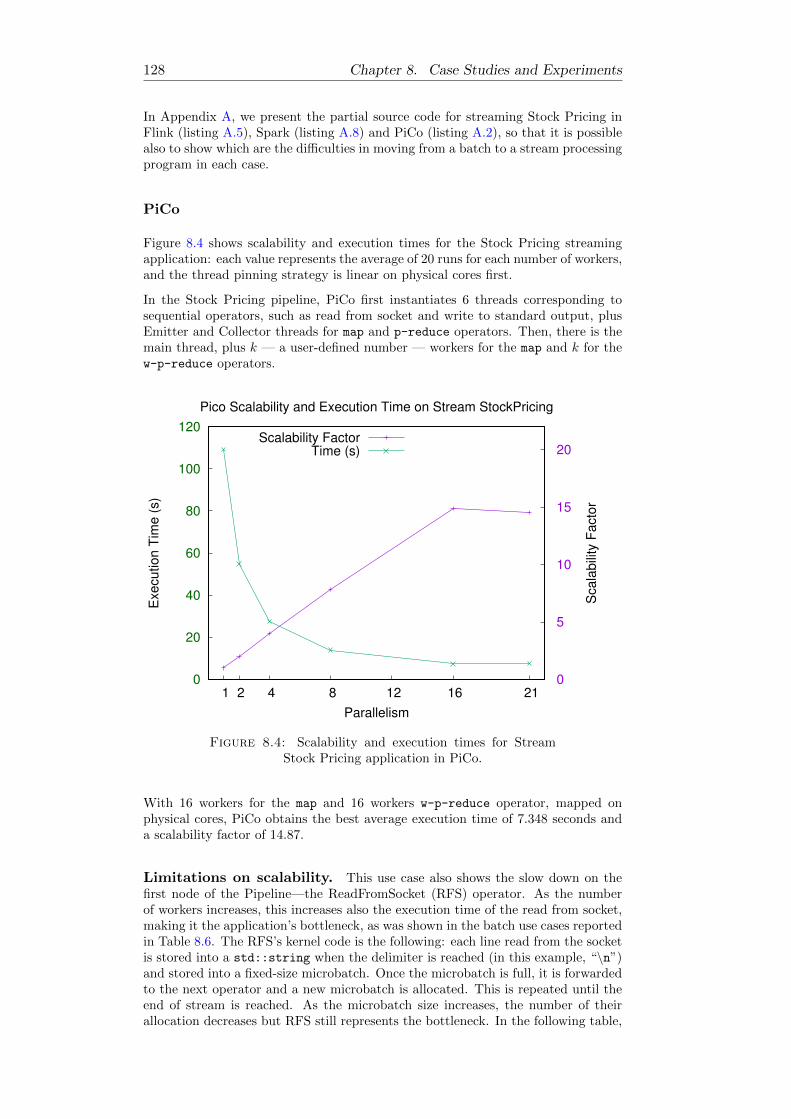
128 Chapter 8. Case Studies and Experiments
In Appendix A, we present the partial source code for streaming Stock Pricing inFlink (listing A.5), Spark (listing A.8) and PiCo (listing A.2), so that it is possiblealso to show which are the difficulties in moving from a batch to a stream processingprogram in each case.
PiCo
Figure 8.4 shows scalability and execution times for the Stock Pricing streamingapplication: each value represents the average of 20 runs for each number of workers,and the thread pinning strategy is linear on physical cores first.
In the Stock Pricing pipeline, PiCo first instantiates 6 threads corresponding tosequential operators, such as read from socket and write to standard output, plusEmitter and Collector threads for map and p-reduce operators. Then, there is themain thread, plus k — a user-defined number — workers for the map and k for thew-p-reduce operators.
0
20
40
60
80
100
120
1 2 4 8 12 16 21 0
5
10
15
20
Exe
cu
tio
n T
ime
(s)
Sca
lab
ility
Fa
cto
r
Parallelism
Pico Scalability and Execution Time on Stream StockPricing
Scalability FactorTime (s)
Figure 8.4: Scalability and execution times for StreamStock Pricing application in PiCo.
With 16 workers for the map and 16 workers w-p-reduce operator, mapped onphysical cores, PiCo obtains the best average execution time of 7.348 seconds anda scalability factor of 14.87.
Limitations on scalability. This use case also shows the slow down on thefirst node of the Pipeline—the ReadFromSocket (RFS) operator. As the numberof workers increases, this increases also the execution time of the read from socket,making it the application’s bottleneck, as was shown in the batch use cases reportedin Table 8.6. The RFS’s kernel code is the following: each line read from the socketis stored into a std::string when the delimiter is reached (in this example, “\n”)and stored into a fixed-size microbatch. Once the microbatch is full, it is forwardedto the next operator and a new microbatch is allocated. This is repeated until theend of stream is reached. As the microbatch size increases, the number of theirallocation decreases but RFS still represents the bottleneck. In the following table,

8.2. Experiments 129
we report execution times of a single run of Stock Pricing with microbatch size512, since previous tests showed that it represents the best granularity for goodperformance. We then compare execution times obtained with the two pinningstrategy (interleaved and linear). The table shows how the scalability on workersis still increasing despite the bottleneck on RFS and how the two different pinningstrategy help in reducing this effect, giving room for improvement on the totalexecution time. We show execution times for a number of workers up to a maximumof 21 for the map and w-p-reduce each, in order to exploit all physical cores of thenode (48).
Interleaved Pinning Strategy (execution time in ms)
workers exec. time read from socket map worker map scalability1 100966.00 3882.59 100966.00 1.002 50870.60 4315.00 50870.00 1.984 28093.00 4576.83 28023.50 3.60
16 8855.81 8847.47 8848.53 11.4121 8753.42 8745.43 8750.95 11.54
Linear Pinning Strategy (execution time in ms)
workers exec. time read from socket map worker map scalability1 109184.00 3962.74 109184.00 1.002 54747.90 3979.72 54747.50 1.994 27426.10 4064.94 27423.40 3.988 13927.80 4245.09 13926.20 7.84
16 7386.69 6341.60 7277.45 15.0021 7548.15 7539.83 7545.49 14.47
Table 8.6: Decomposition of execution times and scalabil-ity highlighting the bottleneck on ReadFromSocket operator.
Comparison with other tools
We compared PiCo to Flink and Spark on the Stock Pricing streaming application.In this section, we provide a comparison on minimum execution time obtained byeach tool as the average of 20 runs for each application, a study on execution timesvariability, and metrics on resources utilization. Configuration used for all tools arethe reported in Table 8.3. We executed PiCo with a maximum of 21 worker threadsfor each data parallel operator (map and w-p-reduce), as previously defined, inorder to exploit the maximum number of physical threads of the node. The windowis count-based (or tumbling) and has size 8 in Flink and PiCo. In Spark, it is notpossible to create count-based windows since only time-based ones are available, sowe created tumbling windows with duration of 10 seconds, by which the executiontime with one thread is similar to PiCo’s one. We have to remark that comparisonwith Spark is not completely fair, since the windowing is not performed in a count-based fashion. To the best of our knowledge, it is not possible to implement suchwindowing policy in Spark.
We briefly recall some aspects of Flink’s and Spark’s runtime. In Flink, each processhas one or more task slots, each of which runs one pipeline of parallel tasks (i.e., thenth instance of a map operator on the n-th partition of the input). The parallelismparameter determines how operations are split into individual tasks, which are as-signed to task slots, that is, it defines parallelism degree for data parallel operators.By setting the parallelism to N , Flink tries to divide an operation into N paralleltasks computed concurrently using the available task slots. The number of taskslots should be equal to the parallelism to ensure that all tasks can be computed ina task slot concurrently but, unfortunately, by setting parallelism to a value greaterthan 32, the program crashes because of insufficient internal resource availability.Due to this limitation, we run Flink with up to 21 worker threads, in order to bealigned with PiCo. We used the same maximum number of threads also in Spark,

130 Chapter 8. Case Studies and Experiments
even though it would be possible to exploit more parallelism: since Spark scalabil-ity in this use case is limited, it is not unfair to be aligned with PiCo’s parallelismexploitation.
For stream processing, Spark implements an extension through the Spark Streamingmodule, providing a high-level abstraction called discretized stream or DStream.Such streams represent results in continuous sequences of RDDs of the same type,called micro-batches. Operations over DStreams are “forwarded” to each RDD inthe DStream, thus the semantics of operations over streams is defined in terms ofbatch processing. All RDDs in a DStream are processed in order, whereas dataitems inside an RDD are processed in parallel without any ordering guarantees.Hence, Spark implements its stream processing runtime over the batch processingone, thus exploiting the BSP runtime on stream microbatches, without providing aconcrete form of pipelining and reducing the real-time processing feature.
Stream Stock Pricing Best Execution Time (ms)
Best exec. time Parallelism ScalabilityFlink 24784.60 16 9.21Spark 42216.21 16 2.24PiCo 7348.58 16 14.87
Table 8.7: Flink, Spark and PiCo best average executiontimes, showing also the scalability with respect to the aver-
age execution time with one thread.
Table 8.7 shows in a summarized manner the best execution times obtained by eachtool, extracted from Table 8.8.
The table shows that PiCo reaches the best execution time with a higher scalabilitywith respect to other tools, with a scalability of 14.87 in PiCo while 9.21 in Flinkand 2.24 Spark.
Table 8.8 also shows the average and the variability of execution times obtained byall the executions. We remark that “parallelism” has different meanings for eachtool, as described in the paragraph above. It shows that, also in this use case, Flinkis slightly less predictable2 than PiCo, reaching a peak of 2.06% for the coefficientof variation.
A strong variability is reported for Spark. We have seen, from the web user in-terface provided by Spark that the input rate from sockets has a great variability,introducing latencies that lead to a reported average of 5 seconds of task schedul-ing delay. Furthermore, it can be noticed that the best average execution time inSpark has a coefficient of variation of 38.90%, with a minimum execution time of 24seconds and a maximum of 74 seconds (values not reported) and that, in all cases,Spark and Flink suffer from scalability issues. PiCo outperforms both Spark andFlink in terms of standard deviation, and outperforms Spark in terms of coefficientof variation. We again validated results with the ANOVA test, which validated ourresults.
2We consider predictability of execution times since the execution happened to fail, aswe reported above in this section.

8.2. Experiments 131
Flink Stream Stock Pricing
Parallelism 1 2 4 8 16 21avg (ms) 228383.40 119669.30 65031.35 36786.20 24784.60 27000.85
sd (s) 1721.24 975.84 525.27 273.85 270.51 556.52cv (%) 0.75 0.81 0.81 0.74 1.09 2.06
avg Scal. 1.00 1.91 3.51 6.21 9.21 8.46
Spark Stream Stock Pricing
Parallelism 1 2 4 8 16 21avg (ms) 94400.00 74059.67 50886.67 52929.17 42216.21 85479.30
sd (s) 8961.03 20207.12 10037.38 5664.81 16424.54 77601.40cv (%) 9.49 27.28 19.72 10.70 38.90 90.78
avg Scal. 1 1.27 1.85 1.78 2.24 1.10
PiCo Stream Stock Pricing
Parallelism 1 2 4 8 16 21avg (ms) 109273.35 54789.40 27532.85 13914.29 7348.58 7536.46
sd (s) 54.96 49.16 147.78 31.68 74.67 45.89cv (%) 0.05 0.09 0.54 0.23 1.02 0.61
avg Scal. 1.00 1.99 3.97 7.85 14.87 14.50
Table 8.8: Average, standard deviation and coefficient ofvariation on 20 runs of the stream Stock Pricing benchmark.
Best execution times are highlighted.
We again measured CPU and memory utilization using the sar tool. We executed10 runs for each configuration: results obtained show a low variability, so thatwe do not report average and variance of collected results. Table 8.9 shows CPUutilization percentages only for average best execution times reported in table 8.8.
Stream Stock Pricing (execution time in ms)
Best exec. time Parallelism CPU (%) RAM (MB)Flink 24784.60 16 14.31% 4875.88Spark 42216.21 16 10.23% 3169.32PiCo 7348.58 16 38.85% 314.57
Table 8.9: User’s percentage usage of all CPUs and RAMused in MB, referred to best execution times.
Flink and Spark show a memory utilization of 4 and 3 GB respectively, that is, oneorder of magnitude greater than PiCo, using only 314 MB and outperforming othertools in resource utilization.
Throughput Values for 10M Stock Options
Best exec. time (s) Parallelism Stocks per SecondFlink 24.78 16 403476.35Spark 42.22 16 236875.81PiCo 7.35 16 1360806.94
Table 8.10: Stream Stock Pricing: Throughput valuescomputed as the number of input stock options with respect
to the best execution time.
Finally, we provide throughput values computed with respect to the number ofstock options in the input stream in the best execution time scenario reported inTable 8.8. We remark that the comparison with Spark is not completely fair sincewindowing is not performed in a count-based fashion. Table 8.10 shows that PiCo

132 Chapter 8. Case Studies and Experiments
processes more than 1.3M stock options per second, outperforming Flink and Spark,which processes about 400K and 200K stock options per second respectively.
8.3 Summary
In this Chapter we provided a set of experiments based on examples defined inSect. 5.4, comprehending both batch and stream applications. We compared PiCoto Flink and Spark, focusing on expressiveness of the programming model andon performances in shared memory. The current experiments are run on sharedmemory only. By comparing execution times in both batch and stream applications,we reached the best execution time when comparing to state-of-the-art frameworksSpark and Flink. Nevertheless, results showed high dynamic allocation contention ininput generation nodes, which limits PiCo scalability. An extension of PiCo usingthe FastFlow allocator might be used by any number of threads to dynamicallyallocate/deallocate memory. We also measured RAM and CPU utilization with thesar tool, which confirmed a lower memory consumption by PiCo with respect tothe other frameworks when compared on batch application (Word Count and StockPricing) and stream application (Stock Pricing streaming): these results rely on thestability of a lightweight C++ runtime, in contrast to Java. What we reported inthis Chapter is a preliminary experimental phase. We re working on providing morerelevant benchmark, such as the Sort/Terasort, and support for HDFS is neededfor such benchmarks.
133
Chapter 9
Conclusions
In this thesis, we presented PiCo, a new C++ DSL for data analytics pipelines. Westarted by studying and analyzing a large number of Big Data analytics tools, amongwhich we identified the most representative ones: Spark [131], Storm [97], Flink [67]and Google Dataflow [5]. By analyzing in depth these frameworks, we identified theDataflow model as the common model that better describes all levels of abstraction,from the user-level API to the execution model. Being all realized under the samecommon idea, we showed how various Big Data analytics tools share almost thesame base concepts, differing mostly in their implementation choices. We theninstantiated the Dataflow model into a stack of layers where each layer representsa dataflow graph/model with a different meaning, describing a program from whatthe programmer sees down to the underlying, lower-level, execution model layer(Chapter 4).
This study led to the specification and formalization of the minimum kernel of op-erations needed to create a pipeline for data analytics. As one of the strength ofPiCo, we implemented a framework in which the data model is also hidden to theprogrammer, thus allowing the possibility to create a model that is polymorphicwith respect to data model and processing model (i.e., stream or batch processing).This make it possible to 1) re-use the same algorithms and pipelines on differentdata models (e.g., stream, lists, sets, etc.); 2) reuse the same operators in differentcontexts, and 3) update operators without affecting the calling context. These as-pects are fundamental for PiCo, since they differentiate it from all other frameworksexposing different data types to be used in the same application, forcing the user tore-think the whole application when moving from one operation to another. Fur-thermore, another goal reached, which is missing in other frameworks which usuallyprovide the API description, is the one of formally defining the syntax of a programbased on Pipelines and operators, hiding the data structures produced and gener-ated by the program as well as providing a semantic interpretation that maps anyPiCo program to a functional Dataflow graph — graph that represents the transfor-mation flow followed by the processed collections (Chapter 5). This is in completecontrast with the unclear approach used by implementors of commercial-orientedBig Data analytics tools.
The formalization step concludes by showing how a PiCo program is compiled intoa graph of parallel processing nodes. The compilation step takes as input the directacyclic dataflow graph (DAG) resulting from a PiCo program (the Semantic DAG)and transforms it, using a set of rules, into a graph that we call the Parallel Execu-tion (PE) Graph, representing a possible parallelization of the Semantic DAG. Weprovided this compilation step in a way that is abstract with respect to any actualimplementation. For instance, it may be implemented in shared memory or througha distributed runtime. Moreover, a compiled (and optimized) Dataflow graph maybe directly mapped to an actual network of computing units (e.g., communicatingthreads or processes) or executed by a macro-Dataflow interpreter (Chapter 6).
We succeed to implement our model into a C++14 compliant DSL whose aim is tofocus on ease of programming with a clear and simple API, exposing to the user

134 Chapter 9. Conclusions
a set of operator objects composed into a Pipeline object, processing bounded orunbounded data. This API was designed to exhibit a functional style over C++14standard by defining a library of purely functional data transformation operatorsexhibiting 1) a well-defined functional and parallel semantics because of our formal-ization and 2) a fluent interface based on method chaining to improve code writingand readability (Chapter 7). Moreover, our API is data-model agnostic, that is, aPiCo program can address both batch and stream processing with a unique API anda unique runtime simply by having the user specify the data source as the first nodeof the Pipeline in a PiCo application. The type system described and implementedwill check if the Pipeline built is compliant with respect to the kind of data beingprocessed.
The current version of PiCo is built to run on shared memory only, but it will bepossible to easily exploit distributed memory platforms thanks to its runtime levelimplemented on top of FastFlow which already supports execution on distributedsystems. Furthermore, we remark that choosing FastFlow as the runtime for PiCogives us almost for free the capability to realize a distributed memory implementa-tion by still maintaining the very same implementation, only by changing communi-cation among processes. To achieve this goal, we will provide an implementation ofthe FastFlow runtime for distributed execution by mean of a Global AsynchronousMemory(GAM) system model. The GAM system consists in a network of execu-tors (i.e., FastFlow workers as well as PiCo operators) accessing a global dynamicmemory with weak sharing semantics, allowing operators to communicate to eachother in predefined communicators where they can exchange C++ smart pointers.
It is also possible to envision exploiting an underlying memory model such as PGASor DSM: since FastFlow moves pointers and not data in communication channelsamong nodes, the same approach can be used to avoid data movement in a dis-tributed scenario with an ad hoc relaxed consistency model. Another goal reach-able by PiCo is the easily offloading of kernels to external devices such as GPU,FPGA, etc. This is possible for two reasons: the first is because of the C++ lan-guage, which naturally targets libraries and API for heterogeneous programming.The second is within the FastFlow runtime and API, which provides support foreasily offloading tasks to GPUs. This is obviously a strength in the choice of imple-menting PiCo in C++ instead of Java/Scala, which also provide libraries for GPUoffloading that are basically wrapper or extension for OpenCL or CUDA, based onauto-generated low-level bindings, but no such library is yet officially recognized asa Java extension.
From the actual performance viewpoint, we aim to solve dynamic allocation con-tention problems we are facing in input generation nodes, as showed in Chapter 8,which limits PiCo scalability. As future work, we could provide PiCo with theFastFlow allocator: this is a specialized allocator that allocates only large chunks ofmemory, slicing them up into little chunks of the same size which can be reused oncefreed. The FastFlow allocator relies on malloc and free, which makes it unfeasibleto be used with C++ Standard Containers and with modern C++ in general. Anextension of the FastFlow allocator in this direction might be used by any numberof threads to dynamically allocate/deallocate memory.
In PiCo, we rely on the stability of a lightweight C++ runtime, in contrast toJava. We measured RAM and CPU utilization with the sar tool, which confirmeda lower memory consumption by PiCo with respect to the other frameworks whencompared on batch application (Word Count and Stock Pricing) and stream ap-plication (Stock Pricing streaming). As another future work, we will provide PiCowith fault tolerance capabilities for automatic restore in case of failures. Anotherimprovement for PiCo implementation on distributed systems would be to exploitthe very same runtime on PGAS or DSMs, in order to still be able to use FastFlow’scharacteristic of moving pointers instead of data, thus allowing a high portability

Chapter 9. Conclusions 135
at the cost of just managing communication among actors in a different memorymodel, which is left to the runtime.
In the experiments chapter, we showed that we achieved the goal of having alightweight runtime able to better exploit resources (outperforming in memory uti-lization), obtaining a better execution time on benchmarks we tested with respectto Flink and Spark, which are two the most used tools nowadays. PiCo obtainedgood results even though it is still in a prototype phase, ensuring that it will bepossible for us to still improve performances by providing special allocators to re-duce dynamic memory allocation contentions, one the current performance issue inPiCo (Chapter 8).
With this thesis we aimed at bringing some order to the confused world of Big Dataanalytics, and we hope the readers will agree that we have reached our goal—atleast in part. We believe that PiCo makes a step forward by giving C++ a chanceof entering into a world almost completely Java-dominated—often considered moreuser-friendly. Starting from our preliminary work, we can envision a complete C++framework that will provide all expected features of a fully equipped environmentand that can be easily used by the data analytics scientists community.


137
Appendix A
Source Code
In this Appendix we provide source code snapshots reporting classes related to thecore operations of each application.
PiCo
Stock Pricing
1 Pipe stockPricing((ReadFromFile()));
2 stockPricing
3 .to(blackScholes).add(PReduce<StockAndPrice>([]
4 (StockAndPrice p1, StockAndPrice p2){
5 return std::max(p1,p2);}))
6 .add(WriteToDisk<StockAndPrice>([](StockAndPrice kv){
7 return kv.to_string();
8 }));
9
10 /* execute the pipeline */
11 stockPricing.run();
Listing A.1: Batch Stock Pricing C++ pipeline inPiCo.
1 size_t window_size = 8;
2 Pipe stockPricing(ReadFromSocket(’\n’));
3 stockPricing
4 .to(varianceMap).add(PReduce<StockAndPrice>([]
5 (StockAndPrice p1, StockAndPrice p2) {
6 return std::max(p1,p2);
7 })
8 .window(window_size))
9 .add(WriteToStdOut<StockAndPrice>([](StockAndPrice kv)
10 {return kv.to_string();}
11 ));
12
13 /* execute the pipeline */
14 stockPricing.run();
15
Listing A.2: Stream Stock Pricing C++ pipeline inPiCo.

138 Appendix A. Source Code
Flink
Word Count
1 public class WordCount {
2 // set up the execution environment
3 final ExecutionEnvironment env =
4 ExecutionEnvironment.getExecutionEnvironment();
5 // get input data
6 DataSet<String> text = env.readTextFile(params.get("input"));
7
8 DataSet<Tuple2<String, Integer>> counts =
9 // split up the lines in pairs (2-tuples) containing: (word,1)
10 text.flatMap(new Tokenizer())
11 // group by the tuple field "0" and sum up tuple field "1"
12 .groupBy(0)
13 .sum(1);
14
15 // emit result
16 if (params.has("output")) {
17 counts.writeAsCsv(params.get("output"), "\n", " ");
18 env.execute("WordCount Example");
19 } else {
20 System.out.println("Printing result to stdout. Use --output to specify
output path.");
21 counts.print();
22 }
23
24 /**
25 * Implements the string tokenizer that splits sentences into words as a user-
defined
26 * FlatMapFunction. The function takes a line (String) and splits it into
27 * multiple pairs in the form of "(word,1)" ({@code Tuple2<String, Integer>}).
28 */
29 public static final class Tokenizer
30 implements FlatMapFunction<String, Tuple2<String, Integer>> {
31 @Override
32 public void flatMap(String value, Collector<Tuple2<String, Integer>> out)
33 {
34 // normalize and split the line
35 String[] tokens = value.toLowerCase().split("\\W+");
36 // emit the pairs
37 for (String token : tokens) {
38 if (token.length() > 0) {
39 out.collect(new Tuple2<String, Integer>(token, 1));
40 }
41 }
42 }
43 }
44 }
Listing A.3: Word Count Java class in Flink.

Appendix A. Source Code 139
Stock Pricing
1 public class StockPricing {
2 // set up the execution environment
3 final ExecutionEnvironment env =
4 ExecutionEnvironment.getExecutionEnvironment();
5 DataSet<String> text = env.readTextFile(params.get("input"));
6 DataSet<Tuple2<String, Double>> max_prices =
7 // parse the lines in pairs containing: (stock,option)
8 text.map(new OptionParser())
9 // compute the price of each stock option
10 .map(new BlackScholes())
11 // group by the tuple field "0" and extracts max on tuple field "1"
12 .groupBy(0).max(1);
13
14 // emit result
15 if (params.has("output")) {
16 max_prices.writeAsCsv(params.get("output"), "\n", " ");
17 env.execute("StockPricing Example");
18 } else {
19 System.out.println("Printing result to stdout. Use --output to specify
output path.");
20 max_prices.print();
21 }
22 }
Listing A.4: Batch Stock Pricing Java class in Flink.
1 // get the execution environment
2 final StreamExecutionEnvironment env = StreamExecutionEnvironment.
getExecutionEnvironment();
3 env.setBufferTimeout(20);
4
5 // get input data by connecting to the socket
6 DataStream<String> text = env.socketTextStream("localhost", port, "\n");
7
8 DataStream<Tuple2<String, Double>> max_prices =
9 // parse the lines in pairs containing: (stock,option)
10 text.map(new OptionParser())
11 // compute the price of each stock option
12 .map(new varianceMap())
13 // group by the tuple field "0" and extracts max on
14 // tuple field "1"
15 .keyBy(0).countWindow(8).max(1);
16
17 // print the results with a single thread, rather than in parallel
18 max_prices.print().setParallelism(1);
Listing A.5: Stream Stock Pricing Java class in Flink.
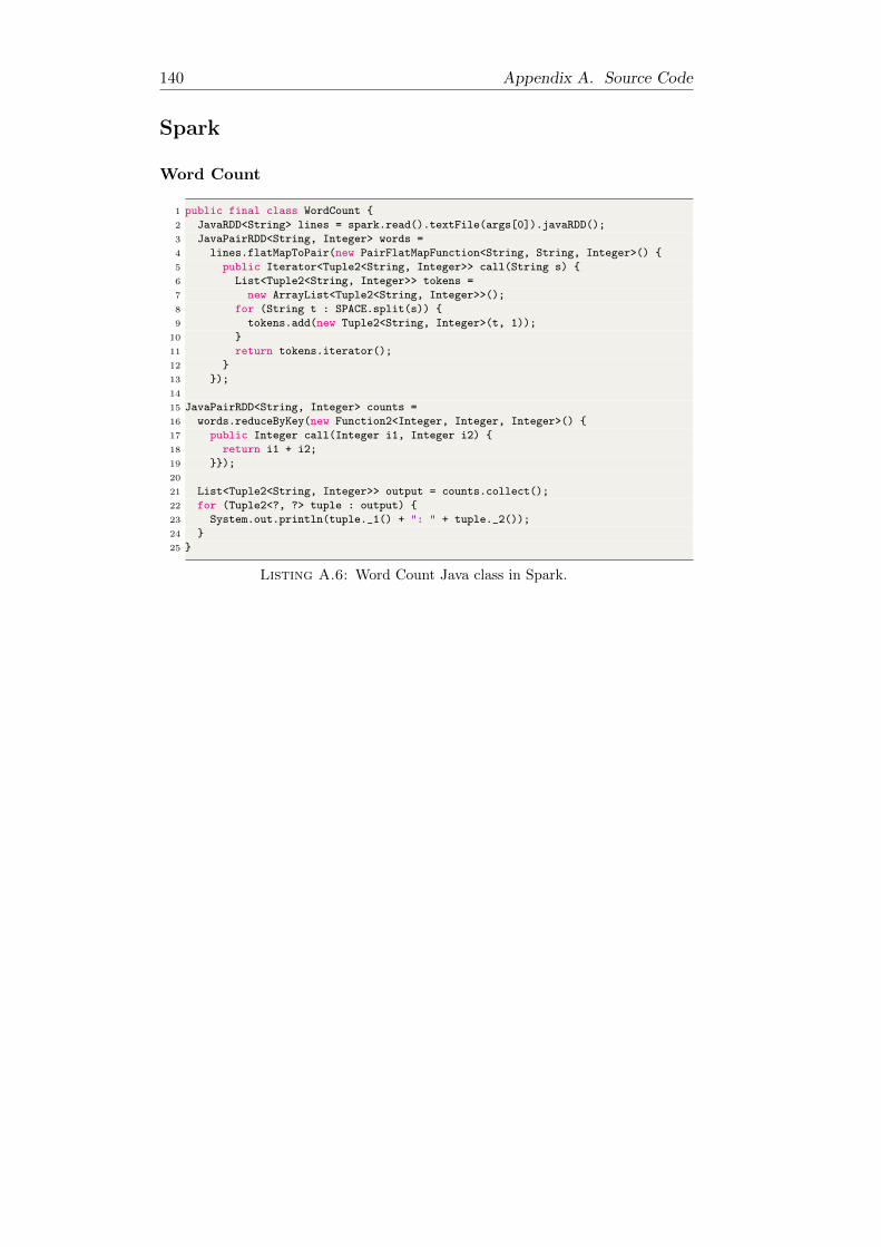
140 Appendix A. Source Code
Spark
Word Count
1 public final class WordCount {
2 JavaRDD<String> lines = spark.read().textFile(args[0]).javaRDD();
3 JavaPairRDD<String, Integer> words =
4 lines.flatMapToPair(new PairFlatMapFunction<String, String, Integer>() {
5 public Iterator<Tuple2<String, Integer>> call(String s) {
6 List<Tuple2<String, Integer>> tokens =
7 new ArrayList<Tuple2<String, Integer>>();
8 for (String t : SPACE.split(s)) {
9 tokens.add(new Tuple2<String, Integer>(t, 1));
10 }
11 return tokens.iterator();
12 }
13 });
14
15 JavaPairRDD<String, Integer> counts =
16 words.reduceByKey(new Function2<Integer, Integer, Integer>() {
17 public Integer call(Integer i1, Integer i2) {
18 return i1 + i2;
19 }});
20
21 List<Tuple2<String, Integer>> output = counts.collect();
22 for (Tuple2<?, ?> tuple : output) {
23 System.out.println(tuple._1() + ": " + tuple._2());
24 }
25 }
Listing A.6: Word Count Java class in Spark.

Appendix A. Source Code 141
Stock Pricing
1 JavaRDD<String> lines = spark.read().textFile(args[0]).javaRDD();
2
3 JavaPairRDD<String, OptionData> stock_options =
4 lines.mapToPair(new PairFunction<String, String, OptionData>() {
5 public Tuple2<String, OptionData> call(String value) {
6 // tokenize the line
7 String[] tokens = value.split("[\t ]");
8 int i = 0;
9 // parse stock name
10 String name = tokens[i++];
11 // parse option data
12 OptionData opt = new OptionData();
13 // parsing options..
14 return new Tuple2<String, OptionData>(name, opt);
15 }
16 });
17
18 JavaPairRDD<String, Double> stock_prices=stock_options.mapToPair(new
BlackScholes());
19
20 JavaPairRDD<String, Double> counts =
21 stock_prices.reduceByKey( new Function2<Double, Double, Double>() {
22 public Double call(Double i1, Double i2) {
23 return i1 + i2;
24 }
25 });
26
27 List<Tuple2<String, Double>> output = counts.collect();
28 for (Tuple2<?,?> tuple : output) {
29 System.out.println(tuple._1() + ": " + tuple._2());
30 }
31
Listing A.7: Batch Stock Pricing Java class in Spark.
1 // Create a DStream that will connect to hostname:port
2 JavaReceiverInputDStream<String> lines = jssc.socketTextStream("localhost",
4000, StorageLevels.MEMORY_AND_DISK_SER);
3
4
5 @SuppressWarnings("serial")
6 JavaPairDStream<String, OptionData> stock_options = lines //
7 .mapToPair(new PairFunction<String, String, OptionData>() {
8 public Tuple2<String, OptionData> call(String value) {
9 // tokenize the line
10 String[] tokens = value.split("[\t ]");
11 int i = 0;
12
13 // parse stock name
14 String name = tokens[i++];
15
16 OptionData opt = new OptionData();
17 // parse option data ...
18 return new Tuple2<String, OptionData>(name, opt);
19 }
20 });
21
22 JavaPairDStream<String, Double> stock_prices = stock_options //
23 .mapToPair(new varianceMap());
24
25 JavaPairDStream<String, Double> counts = stock_prices.reduceByKey(new Function2<
Double, Double, Double>() {
26 public Double call(Double i1, Double i2) {
27 return Math.max(i1, i2);
28 }
29 });
Listing A.8: Stream Stock Pricing Java class in Spark.


143
Bibliography
[1] IEEE standard for floating-point arithmetic. IEEE Std 754-2008, pages 1–70,Aug 2008.
[2] M. Abadi et al. TensorFlow: Large-Scale Machine Learning on HeterogeneousSystems. http://tensorflow.org/, 2015.
[3] M. Abadi and M. Isard. Timely dataflow: A model. In FORTE, pages 131–145, 2015.
[4] S. V. Adve and K. Gharachorloo. Shared memory consistency models: Atutorial. Computer, 29(12):66–76, Dec. 1996.
[5] T. Akidau, R. Bradshaw, C. Chambers, S. Chernyak, R. J. Fernandez-Moctezuma, R. Lax, S. McVeety, D. Mills, F. Perry, E. Schmidt, and S. Whit-tle. The dataflow model: A practical approach to balancing correctness, la-tency, and cost in massive-scale, unbounded, out-of-order data processing.Proc. VLDB Endow., 8(12):1792–1803, Aug. 2015.
[6] T. Akidau, R. Bradshaw, C. Chambers, S. Chernyak, R. J. Fernandez-Moctezuma, R. Lax, S. McVeety, D. Mills, F. Perry, E. Schmidt, and S. Whit-tle. The dataflow model: A practical approach to balancing correctness, la-tency, and cost in massive-scale, unbounded, out-of-order data processing.Proceedings of the VLDB Endowment, 8:1792–1803, 2015.
[7] M. Aldinucci. eskimo: experimenting with skeletons in the shared addressmodel. Parallel Processing Letters, 13(3):449–460, Sept. 2003.
[8] M. Aldinucci, S. Bagnasco, S. Lusso, P. Pasteris, and S. Rabellino. The OpenComputing Cluster for Advanced data Manipulation (occam). In The 22ndInternational Conference on Computing in High Energy and Nuclear Physics(CHEP), San Francisco, USA, Oct. 2016.
[9] M. Aldinucci, S. Campa, P. Ciullo, M. Coppola, S. Magini, P. Pesciullesi,L. Potiti, R. Ravazzolo, M. Torquati, M. Vanneschi, and C. Zoccolo. Theimplementation of ASSIST, an environment for parallel and distributed pro-gramming. In H. Kosch, L. Boszormenyi, and H. Hellwagner, editors, Proc.of 9th Intl Euro-Par 2003 Parallel Processing, volume 2790 of LNCS, pages712–721, Klagenfurt, Austria, Aug. 2003. Springer.
[10] M. Aldinucci, M. Coppola, M. Danelutto, M. Vanneschi, and C. Zoccolo. AS-SIST as a research framework for high-performance grid programming envi-ronments. In J. C. Cunha and O. F. Rana, editors, Grid Computing: Softwareenvironments and Tools, chapter 10, pages 230–256. Springer, Jan. 2006.
[11] M. Aldinucci and M. Danelutto. Skeleton based parallel programming: func-tional and parallel semantic in a single shot. Computer Languages, Systemsand Structures, 33(3-4):179–192, Oct. 2007.
[12] M. Aldinucci, M. Danelutto, M. Drocco, P. Kilpatrick, Claudia Misale,G. Peretti Pezzi, and M. Torquati. A parallel pattern for iterative stencil +reduce. Journal of Supercomputing, pages 1–16, 2016.
[13] M. Aldinucci, M. Danelutto, and P. Kilpatrick. Towards hierarchical manage-ment of autonomic components: a case study. In D. E. Baz, T. Gross, and

144 BIBLIOGRAPHY
F. Spies, editors, Proc. of Intl. Euromicro PDP 2009: Parallel Distributed andnetwork-based Processing, pages 3–10, Weimar, Germany, Feb. 2009. IEEE.
[14] M. Aldinucci, M. Danelutto, P. Kilpatrick, M. Meneghin, and M. Torquati.An efficient unbounded lock-free queue for multi-core systems. In Proc. of18th Intl. Euro-Par 2012 Parallel Processing, volume 7484 of LNCS, pages662–673, Rhodes Island, Greece, Aug. 2012. Springer.
[15] M. Aldinucci, M. Danelutto, P. Kilpatrick, and M. Torquati. Fastflow: high-level and efficient streaming on multi-core. In S. Pllana and F. Xhafa, ed-itors, Programming Multi-core and Many-core Computing Systems, Paralleland Distributed Computing, chapter 13. Wiley, Oct. 2014.
[16] M. Aldinucci, M. Danelutto, and P. Teti. An advanced environment support-ing structured parallel programming in Java. Future Generation ComputerSystems, 19(5):611–626, July 2003.
[17] M. Aldinucci, M. Drocco, G. Peretti Pezzi, Claudia Misale, F. Tordini,and M. Torquati. Exercising high-level parallel programming on streams: asystems biology use case. In Proc. of the 2014 IEEE 34th Intl. Conference onDistributed Computing Systems Workshops (ICDCS), Madrid, Spain, 2014.IEEE.
[18] M. Aldinucci, M. Meneghin, and M. Torquati. Efficient Smith-Waterman onmulti-core with fastflow. In M. Danelutto, T. Gross, and J. Bourgeois, editors,Proc. of Intl. Euromicro PDP 2010: Parallel Distributed and network-basedProcessing, pages 195–199, Pisa, Italy, Feb. 2010. IEEE.
[19] M. Aldinucci and M. Torquati. FastFlow website, 2009. http://
mc-fastflow.sourceforge.net/.
[20] M. Aldinucci, M. Torquati, C. Spampinato, M. Drocco, Claudia Misale,C. Calcagno, and M. Coppo. Parallel stochastic systems biology in the cloud.Briefings in Bioinformatics, 15(5):798–813, 2014.
[21] A. Alexandrov, R. Bergmann, S. Ewen, J.-C. Freytag, F. Hueske, A. Heise,O. Kao, M. Leich, U. Leser, V. Markl, F. Naumann, M. Peters,A. Rheinlander, M. J. Sax, S. Schelter, M. Hoger, K. Tzoumas, andD. Warneke. The stratosphere platform for big data analytics. The VLDBJournal, 23(6):939–964, Dec. 2014.
[22] Apache Software Foundation. Hadoop, 2013. http://hadoop.apache.org/.
[23] Apache Software Foundation. HDFS, 2013. http://hadoop.apache.org/
docs/r1.2.1/hdfs_user_guide.html.
[24] Apache Software Foundation. Cassandra, 2016. http://cassandra.apache.org.
[25] Apache Software Foundation. HBase, 2016. http://hbase.apache.org/.
[26] Apache Software Foundation. Yarn, 2016. https://hadoop.apache.org/
docs/r2.7.1/hadoop-yarn/hadoop-yarn-site/YARN.html.
[27] Apache Software Foundation. ZooKeeper, 2016. http://zookeeper.apache.org/.
[28] K. Arvind and R. S. Nikhil. Executing a program on the MIT tagged-tokendataflow architecture. IEEE Trans. Comput., 39(3):300–318, Mar. 1990.
[29] K. Asanovic, R. Bodik, J. Demmel, T. Keaveny, K. Keutzer, J. Kubiatowicz,N. Morgan, D. Patterson, K. Sen, J. Wawrzynek, D. Wessel, and K. Yelick.A view of the parallel computing landscape. Communications of the ACM,52(10):56–67, 2009.

BIBLIOGRAPHY 145
[30] S. Bahrampour, N. Ramakrishnan, L. Schott, and M. Shah. Compara-tive study of caffe, neon, theano, and torch for deep learning. CoRR,abs/1511.06435, 2015.
[31] Basho. Riak, 2016. http://basho.com/riak/.
[32] M. A. Beyer and D. Laney. The importance of big data: A definition. Tech-nical report, Stamford, CT: Gartner, June 2012.
[33] R. Bhardwaj, A. Sethi, and R. Nambiar. Big data in genomics: An overview.In 2014 IEEE International Conference on Big Data (Big Data), pages 45–49,Oct 2014.
[34] T. Bingmann, M. Axtmann, E. Jobstl, S. Lamm, H. C. Nguyen, A. Noe,S. Schlag, M. Stumpp, T. Sturm, and P. Sanders. Thrill: High-performance algorithmic distributed batch data processing with C++. CoRR,abs/1608.05634, 2016.
[35] H. Bischof, S. Gorlatch, and R. Leshchinskiy. DatTel: A data-parallel C++template library. Parallel Processing Letters, 13(3):461–472, 2003.
[36] H.-J. Boehm. Threads cannot be implemented as a library. SIGPLAN Not.,40(6):261–268, June 2005.
[37] H.-J. Boehm and S. V. Adve. Foundations of the c++ concurrency memorymodel. In Proceedings of the 29th ACM SIGPLAN Conference on Program-ming Language Design and Implementation, PLDI ’08, pages 68–78, NewYork, NY, USA, 2008. ACM.
[38] J. Bonwick and S. Microsystems. The slab allocator: An object-caching kernelmemory allocator. In In USENIX Summer, pages 87–98, 1994.
[39] E. A. Brewer. Towards robust distributed systems (abstract). In Proceed-ings of the Nineteenth Annual ACM Symposium on Principles of DistributedComputing, PODC ’00, pages 7–, New York, NY, USA, 2000. ACM.
[40] D. R. Butenhof. Programming with POSIX Threads. Addison-Wesley Long-man Publishing Co., Inc., Boston, MA, USA, 1997.
[41] F. Cappello and D. Etiemble. MPI versus MPI+OpenMP on IBM SP for theNAS benchmarks. In Proc. of the 2000 ACM/IEEE conference on Supercom-puting (CDROM), Supercomputing ’00. IEEE Computer Society, 2000.
[42] P. Carbone, G. Fora, S. Ewen, S. Haridi, and K. Tzoumas. Lightweightasynchronous snapshots for distributed dataflows. CoRR, abs/1506.08603,2015.
[43] C. Chambers, A. Raniwala, F. Perry, S. Adams, R. Henry, R. Bradshaw,and Nathan. FlumeJava: Easy, efficient data-parallel pipelines. In ACMSIGPLAN Conference on Programming Language Design and Implementation(PLDI), pages 363–375, 2 Penn Plaza, Suite 701 New York, NY 10121-0701,2010.
[44] K. M. Chandy and L. Lamport. Distributed snapshots: Determining globalstates of distributed systems. ACM Trans. Comput. Syst., 3(1):63–75, Feb.1985.
[45] B. Choi, R. Komuravelli, H. Sung, R. Smolinski, N. Honarmand, S. V. Adve,V. S. Adve, N. P. Carter, and C.-T. Chou. Denovo: Rethinking the memoryhierarchy for disciplined parallelism. In Proceedings of the 2011 InternationalConference on Parallel Architectures and Compilation Techniques, PACT ’11,pages 155–166, Washington, DC, USA, 2011. IEEE Computer Society.

146 BIBLIOGRAPHY
[46] P. Ciechanowicz, M. Poldner, and H. Kuchen. The Munster skeleton libraryMuesli — a comprehensive overview. In ERCIS Working paper, number 7.ERCIS – European Research Center for Information Systems, 2009.
[47] C. Cole and M. Herlihy. Snapshots and software transactional memory. Sci.Comput. Program., 58(3):310–324, 2005.
[48] M. Cole. Algorithmic Skeletons: Structured Management of Parallel Compu-tation. MIT Press, 1991.
[49] M. Cole. Bringing skeletons out of the closet: A pragmatic manifesto forskeletal parallel programming. Parallel Computing, 30(3):389–406, 2004.
[50] M. Cole. Skeletal Parallelism home page, 2009. http://homepages.inf.ed.ac.uk/mic/Skeletons/.
[51] R. Collobert, K. Kavukcuoglu, and C. Farabet. Torch7: A matlab-like envi-ronment for machine learning. In BigLearn, NIPS Workshop, 2011.
[52] Crunch. Apache Crunch website. http://crunch.apache.org/.
[53] M. Danelutto, R. D. Meglio, S. Orlando, S. Pelagatti, and M. Vanneschi.A methodology for the development and the support of massively parallelprograms. Future Generation Compututer Systems, 8(1-3):205–220, 1992.
[54] M. Danelutto and M. Stigliani. SKElib: parallel programming with skeletonsin C. In A. Bode, T. Ludwing, W. Karl, and R. Wismuller, editors, Proc.of 6th Intl. Euro-Par 2000 Parallel Processing, volume 1900 of LNCS, pages1175–1184, Munich, Germany, Aug. 2000. Springer.
[55] M. Danelutto and M. Torquati. Loop parallelism: a new skeleton perspectiveon data parallel patterns. In M. Aldinucci, D. D’Agostino, and P. Kilpatrick,editors, Proc. of Intl. Euromicro PDP 2014: Parallel Distributed and network-based Processing, Torino, Italy, 2014. IEEE.
[56] M. Danelutto and M. Torquati. Structured parallel programming with “core”fastflow. In V. Zsok, Z. Horvath, and L. Csato, editors, Central EuropeanFunctional Programming School, volume 8606 of LNCS, pages 29–75. Springer,2015.
[57] J. Darlington, A. J. Field, P. Harrison, P. H. J. Kelly, D. W. N. Sharp, R. L.While, and Q. Wu. Parallel programming using skeleton functions. In Proc.of Parallel Architectures and Langauges Europe (PARLE’93), volume 694 ofLNCS, pages 146–160, Munich, Germany, June 1993. Springer.
[58] J. Darlington, Y.-k. Guo, H. W. To, and J. Yang. Parallel skeletons for struc-tured composition. In Proceedings of the Fifth ACM SIGPLAN Symposium onPrinciples and Practice of Parallel Programming, PPOPP ’95, pages 19–28,New York, NY, USA, 1995. ACM.
[59] Databricks. Spark Tungsten website. https://databricks.com/blog/2015/04/28/project-tungsten-bringing-spark-closer-to-bare-metal.
html.
[60] T. De Matteis and G. Mencagli. Parallel patterns for window-based statefuloperators on data streams: an algorithmic skeleton approach. InternationalJournal of Parallel Programming, pages 1–20, 2016.
[61] J. Dean and S. Ghemawat. MapReduce: Simplified data processing on largeclusters. In Usenix OSDI ’04, pages 137–150, Dec. 2004.

BIBLIOGRAPHY 147
[62] D. del Rio Astorga, M. F. Dolz, L. M. Sanchez, J. G. Blas, and J. D. Garcıa.A C++ generic parallel pattern interface for stream processing. In Algo-rithms and Architectures for Parallel Processing - 16th International Con-ference, ICA3PP 2016, Granada, Spain, December 14-16, 2016, Proceedings,pages 74–87, 2016.
[63] M. Drocco, Claudia Misale, and M. Aldinucci. A cluster-as-accelerator ap-proach for SPMD-free data parallelism. In Proc. of Intl. Euromicro PDP 2016:Parallel Distributed and network-based Processing, pages 350–353, Crete,Greece, 2016. IEEE.
[64] M. Drocco, Claudia Misale, G. Peretti Pezzi, F. Tordini, and M. Aldinucci.Memory-optimised parallel processing of Hi-C data. In Proc. of Intl. Euromi-cro PDP 2015: Parallel Distributed and network-based Processing, pages 1–8.IEEE, Mar. 2015.
[65] M. Drocco, Misale, Claudia, G. Tremblay, and M. Aldinucci. A formal se-mantics for data analytics pipelines. https://arxiv.org/abs/1705.01629, May2017.
[66] J. Enmyren and C. W. Kessler. Skepu: A multi-backend skeleton program-ming library for multi-GPU systems. In Proceedings of the Fourth Interna-tional Workshop on High-level Parallel Programming and Applications, HLPP’10, pages 5–14, New York, NY, USA, 2010. ACM.
[67] Flink. Apache Flink website. https://flink.apache.org/.
[68] Flink. Flink streaming examples, 2015. [Online; accessed 16-November-2016].
[69] M. J. Flynn. Very high-speed computing systems. Proceedings of the IEEE,54(12):1901–1909, 1966.
[70] M. Fowler. Kappa-Architecture website. https://www.martinfowler.com/
bliki/FluentInterface.html.
[71] H. Gonzalez-Velez and M. Leyton. A survey of algorithmic skeleton frame-works: High-level structured parallel programming enablers. Software: Prac-tice and Experience, 40(12):1135–1160, Nov. 2010.
[72] Google. Google Cloud Dataflow, 2015. https://cloud.google.com/
dataflow/.
[73] J. L. Hennessy and D. A. Patterson. Computer Architecture: A QuantitativeApproach. Elsevier, fifth edition, 2011.
[74] M. Herlihy and N. Shavit. The Art of Multiprocessor Programming. MorganKaufmann Publishers Inc., San Francisco, CA, USA, 2008.
[75] IBM. What is big data? http://www-01.ibm.com/software/data/
bigdata/what-is-big-data.html, 2013.
[76] Intel. Intel R© C++ Intrinsics Reference, 2010.
[77] Intel. Intel R© AVX-512 instructions, 2013. https://software.intel.com/
en-us/blogs/2013/avx-512-instructions.
[78] Intel Corp. Threading Building Blocks, 2011.
[79] M. Isard, M. Budiu, Y. Yu, A. Birrell, and D. Fetterly. Dryad: Distributeddata-parallel programs from sequential building blocks. In Proceedings ofthe 2Nd ACM SIGOPS/EuroSys European Conference on Computer Systems2007, EuroSys ’07, pages 59–72, New York, NY, USA, 2007. ACM.

148 BIBLIOGRAPHY
[80] J. Jeffers and J. Reinders. Front-matter. In J. Jeffers and J. Reinders, editors,Intel Xeon Phi Coprocessor High Performance Programming, pages i – iii.Morgan Kaufmann, Boston, 2013.
[81] D. R. Jefferson. Virtual time. ACM Trans. Program. Lang. Syst., 7(3):404–425, July 1985.
[82] Y. Jia, E. Shelhamer, J. Donahue, S. Karayev, J. Long, R. Girshick,S. Guadarrama, and T. Darrell. Caffe: Convolutional architecture for fastfeature embedding. arXiv preprint arXiv:1408.5093, 2014.
[83] G. Kahn. The semantics of a simple language for parallel programming. InJ. L. Rosenfeld, editor, Information processing, pages 471–475, Stockholm,Sweden, 1974. North Holland, Amsterdam.
[84] Kappa-Architecture. Kappa-Architecture website. http://milinda.
pathirage.org/kappa-architecture.com/.
[85] Khronos Compute Working Group. OpenCL, Nov. 2009. http://www.
khronos.org/opencl/.
[86] M. Kiran, P. Murphy, I. Monga, J. Dugan, and S. S. Baveja. Lambda ar-chitecture for cost-effective batch and speed big data processing. In 2015IEEE International Conference on Big Data (Big Data), pages 2785–2792,Oct 2015.
[87] J. Kreps, N. Narkhede, and J. Rao. Kafka: A distributed messaging system forlog processing. In Proceedings of 6th International Workshop on NetworkingMeets Databases (NetDB), Athens, Greece, 2011.
[88] L. Lamport. How to make a multiprocessor computer that correctly executesmultiprocess programs. IEEE Trans. Comput., 28(9):690–691, Sept. 1979.
[89] L. Lamport. Specifying concurrent program modules. ACM Trans. Program.Lang. Syst., 5(2):190–222, 1983.
[90] D. Laney. 3D data management: Controlling data volume, velocity, andvariety. Technical report, META Group, February 2001.
[91] E. A. Lee and T. M. Parks. Dataflow process networks. Proc. of the IEEE,83(5):773–801, 1995.
[92] H. Li. Introduction to Big Data. http://haifengl.github.io/bigdata/,2016.
[93] B. C. Libraries. Boost Serialization documentation webpage.http://www.boost.org/doc/libs/1_63_0/libs/serialization/doc/
serialization.html.
[94] G. Malewicz, M. H. Austern, A. J. Bik, J. C. Dehnert, I. Horn, N. Leiser, andG. Czajkowski. Pregel: A system for large-scale graph processing. In Proceed-ings of the 2010 ACM SIGMOD International Conference on Management ofData, SIGMOD ’10, pages 135–146, New York, NY, USA, 2010. ACM.
[95] K. Matsuzaki, H. Iwasaki, K. Emoto, and Z. Hu. A library of constructiveskeletons for sequential style of parallel programming. In Proc. of the 1stInter. conference on Scalable information systems, InfoScale ’06, New York,NY, USA, 2006. ACM.
[96] D. Murray, F. McSherry, R. Isaacs, M. Isard, P. Barham, and M. Abadi.Naiad: A timely dataflow system. In Proceedings of the 24th ACM Symposiumon Operating Systems Principles (SOSP). ACM, November 2013.

BIBLIOGRAPHY 149
[97] M. A. U. Nasir, G. D. F. Morales, D. Garcıa-Soriano, N. Kourtellis, andM. Serafini. The power of both choices: Practical load balancing for dis-tributed stream processing engines. CoRR, abs/1504.00788, 2015.
[98] J. Nelson, B. Holt, B. Myers, P. Briggs, L. Ceze, S. Kahan, and M. Oskin.Latency-tolerant software distributed shared memory. In Proceedings of the2015 USENIX Conference on Usenix Annual Technical Conference, USENIXATC ’15, pages 291–305, Berkeley, CA, USA, 2015. USENIX Association.
[99] A. Y. Ng, G. Bradski, C.-T. Chu, K. Olukotun, S. K. Kim, Y.-A. Lin, andY. Yu. Map-reduce for machine learning on multicore. In NIPS, 12/20062006.
[100] B. Nicolae, C. H. A. Costa, Claudia Misale, K. Katrinis, and Y. Park.Leveraging adaptative I/O to optimize collective data shuffling patterns forbig data analytics. IEEE Transactions on Parallel and Distributed Systems,PP(99), 2016.
[101] B. Nicolae, C. H. A. Costa, Claudia Misale, K. Katrinis, and Y. Park.Towards memory-optimized data shuffling patterns for big data analytics. InIEEE/ACM 16th Intl. Symposium on Cluster, Cloud and Grid Computing,CCGrid 2016, Cartagena, Colombia, 2016. IEEE.
[102] NVIDIA Corp. CUDA website, June 2013 (last accessed). http://www.
nvidia.com/object/cuda_home_new.html.
[103] S. Oaks and H. Wong. Java Threads. Nutshell handbooks. O’Reilly Media,2004.
[104] Oracle. NoSQL, 2016. http://nosql-database.org/.
[105] P. S. Pacheco. Parallel programming with MPI. Morgan Kaufmann PublishersInc., San Francisco, CA, USA, 1996.
[106] I. Park, M. J. Voss, S. W. Kim, and R. Eigenmann. Parallel programmingenvironment for OpenMP. Scientific Programming, 9:143–161, 2001.
[107] D. A. Patterson and J. L. Hennessy. Computer Organization and Design:The Hardware/Software Interface. Morgan Kaufmann Publishers Inc., SanFrancisco, CA, USA, 3rd edition, 2007.
[108] M. Poldner and H. Kuchen. Scalable farms. In Proc. of Intl. PARCO 2005:Parallel Computing, Malaga, Spain, Sept. 2005.
[109] C. Ranger, R. Raghuraman, A. Penmetsa, G. Bradski, and C. Kozyrakis.Evaluating mapreduce for multi-core and multiprocessor systems. In Proceed-ings of the 2007 IEEE 13th International Symposium on High PerformanceComputer Architecture, HPCA ’07, pages 13–24, Washington, DC, USA, 2007.IEEE Computer Society.
[110] J. H. Rutgers. Programming models for many-core architectures: a co-designapproach. 2014.
[111] L. M. Sanchez, J. Fernandez, R. Sotomayor, and J. D. Garcia. A comparativeevaluation of parallel programming models for shared-memory architectures.In Proceedings of the 2012 IEEE 10th International Symposium on Paral-lel and Distributed Processing with Applications, ISPA ’12, pages 363–370,Washington, DC, USA, 2012. IEEE Computer Society.
[112] A. Secco, I. Uddin, G. Peretti Pezzi, and M. Torquati. Message pass-ing on infiniband RDMA for parallel run-time supports. In M. Aldinucci,D. D’Agostino, and P. Kilpatrick, editors, Proc. of Intl. Euromicro PDP 2014:Parallel Distributed and network-based Processing, Torino, Italy, 2014. IEEE.

150 BIBLIOGRAPHY
[113] J. Serot. Tagged-token data-flow for skeletons. Parallel Processing Letters,11(4):377–392, 2001.
[114] D. B. Skillicorn and D. Talia. Models and languages for parallel computation.ACM Comput. Surv., 30(2):123–169, June 1998.
[115] D. J. Sorin, M. D. Hill, and D. A. Wood. A Primer on Memory Consistencyand Cache Coherence. Morgan & Claypool Publishers, 1st edition, 2011.
[116] M. Steuwer and S. Gorlatch. Skelcl: Enhancing opencl for high-level pro-gramming of multi-GPU systems. In Proceedings of the 12th InternationalConference on Parallel Computing Technologies, pages 258–272, St. Peters-burg, Russia, Oct. 2013.
[117] Storm. Apache Storm website. http://storm.apache.org/.
[118] Claudia Misale. Accelerating bowtie2 with a lock-less concurrency approachand memory affinity. In Proc. of Intl. Euromicro PDP 2014: Parallel Dis-tributed and network-based Processing, Torino, Italy, 2014. IEEE. (Best paperaward).
[119] Claudia Misale, M. Aldinucci, and M. Torquati. Memory affinity in multi-threading: the bowtie2 case study. In Advanced Computer Architectureand Compilation for High-Performance and Embedded Systems (ACACES)– Poster Abstracts, Fiuggi, Italy, 2013. HiPEAC.
[120] Claudia Misale, M. Drocco, M. Aldinucci, and G. Tremblay. A comparisonof big data frameworks on a layered dataflow model. In Proc. of HLPP2016:Intl. Workshop on High-Level Parallel Programming, pages 1–19, Muenster,Germany, July 2016. arXiv.org.
[121] Claudia Misale, M. Drocco, M. Aldinucci, and G. Tremblay. A comparisonof big data frameworks on a layered dataflow model. Parallel ProcessingLetters, 27(01):1740003, 2017.
[122] Claudia Misale, G. Ferrero, M. Torquati, and M. Aldinucci. Sequence align-ment tools: one parallel pattern to rule them all? BioMed Research Interna-tional, 2014.
[123] Theano Development Team. Theano: A Python framework for fast com-putation of mathematical expressions. arXiv e-prints, abs/1605.02688, May2016.
[124] F. Tordini, M. Drocco, Claudia Misale, L. Milanesi, P. Lio, I. Merelli, andM. Aldinucci. Parallel exploration of the nuclear chromosome conformationwith NuChart-II. In Proc. of Intl. Euromicro PDP 2015: Parallel Distributedand network-based Processing. IEEE, Mar. 2015.
[125] F. Tordini, M. Drocco, Claudia Misale, L. Milanesi, P. Lio, I. Merelli,M. Torquati, and M. Aldinucci. NuChart-II: the road to a fast and scal-able tool for Hi-C data analysis. International Journal of High PerformanceComputing Applications (IJHPCA), 2016.
[126] A. Toshniwal, S. Taneja, A. Shukla, K. Ramasamy, J. M. Patel, S. Kulka-rni, J. Jackson, K. Gade, M. Fu, J. Donham, N. Bhagat, S. Mittal, andD. Ryaboy. Storm@twitter. In Proceedings of the 2014 ACM SIGMOD Inter-national Conference on Management of Data, SIGMOD ’14, pages 147–156,New York, NY, USA, 2014. ACM.
[127] UniTo-INFN. Occam Supercomputer website. http://c3s.unito.it/
index.php/super-computer.
[128] L. G. Valiant. A bridging model for parallel computation. CACM, 33(8):103–111, Aug. 1990.

BIBLIOGRAPHY 151
[129] O. Villa, V. Gurumoorthi, A. Marquez, and S. Krishnamoorthy. Effects offloating-point non-associativity on numerical computations on massively mul-tithreaded systems. In In Cray User Group meeting, CUG’09, 2009.
[130] T. White. Hadoop: The Definitive Guide. O’Reilly Media, Inc., 1st edition,2009.
[131] M. Zaharia, M. Chowdhury, T. Das, A. Dave, J. Ma, M. McCauley, M. J.Franklin, S. Shenker, and I. Stoica. Resilient Distributed Datasets: A Fault-tolerant Abstraction for In-memory Cluster Computing. In Proc. of the9th USENIX Conference on Networked Systems Design and Implementation,NSDI’12, Berkeley, CA, USA, 2012. USENIX.
[132] M. Zaharia, M. Chowdhury, M. J. Franklin, S. Shenker, and I. Stoica. Spark:Cluster computing with working sets. In Proceedings of the 2nd USENIXConference on Hot Topics in Cloud Computing, HotCloud’10, pages 10–10,Berkeley, CA, USA, 2010. USENIX Association.
[133] M. Zaharia, T. Das, H. Li, T. Hunter, S. Shenker, and I. Stoica. Discretizedstreams: Fault-tolerant streaming computation at scale. In Proc. of the 24thACM Symposium on Operating Systems Principles, SOSP, pages 423–438,New York, NY, USA, 2013. ACM.
[134] ZeroMQ. website, 2012. http://www.zeromq.org/.