physics graphing using open office. advantages of graphing with spreadsheet programs can be fast....
TRANSCRIPT
Physics Graphing Using Open Office

Advantages of Graphing with Spreadsheet Programs
• Can be fast. Handles lots of data and multiple calculations.
• Precise calculation of equations.
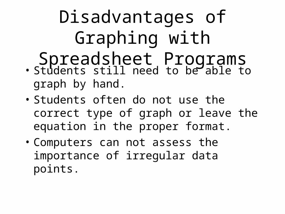
Disadvantages of Graphing with Spreadsheet Programs
• Students still need to be able to graph by hand.
• Students often do not use the correct type of graph or leave the equation in the proper format.
• Computers can not assess the importance of irregular data points.

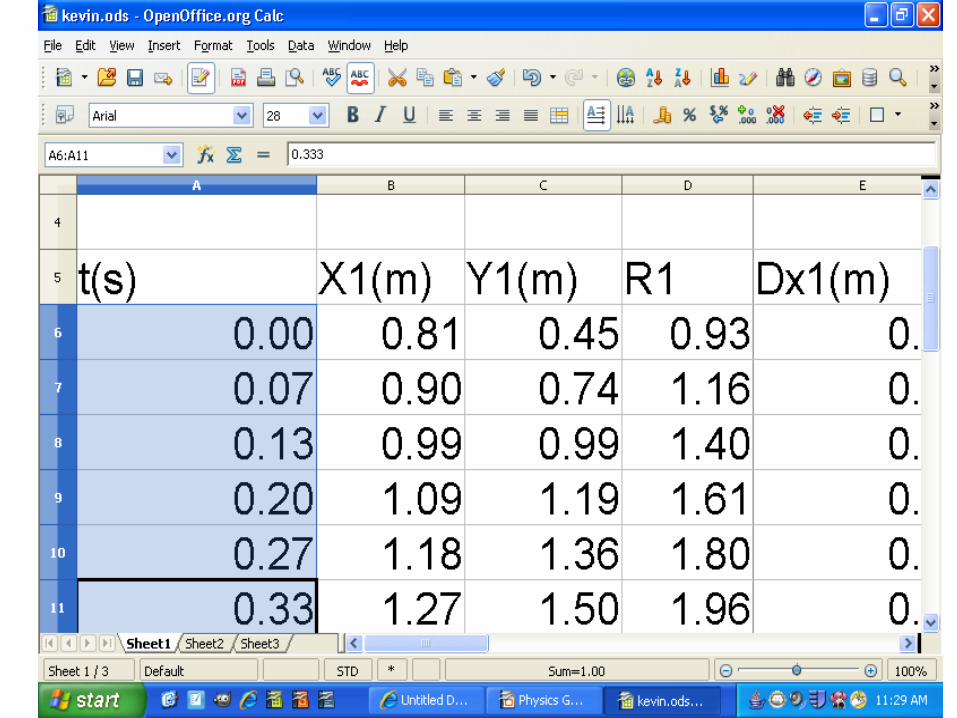
To graph data, it must be inputted into a spreadsheet program.Here is an example of data
collected by a student.


Change format: start by select all
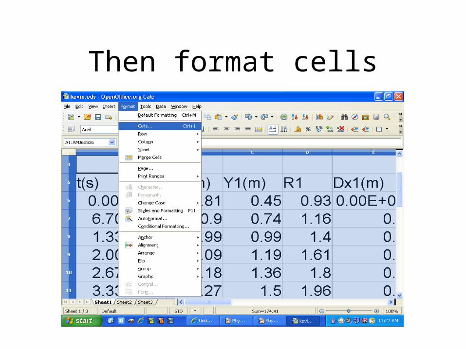
Then format cells

Then choose a reasonable format

To select the data to be graphed, left click on the first cell with the data you want on the x-axis and hold down the button while you move down over the data. To
select the y-data, hold down the ctrl button then left click and
drag down.

Click on Insert then Chart once the data has been selected.

Select x-y scatter plot with no lines.

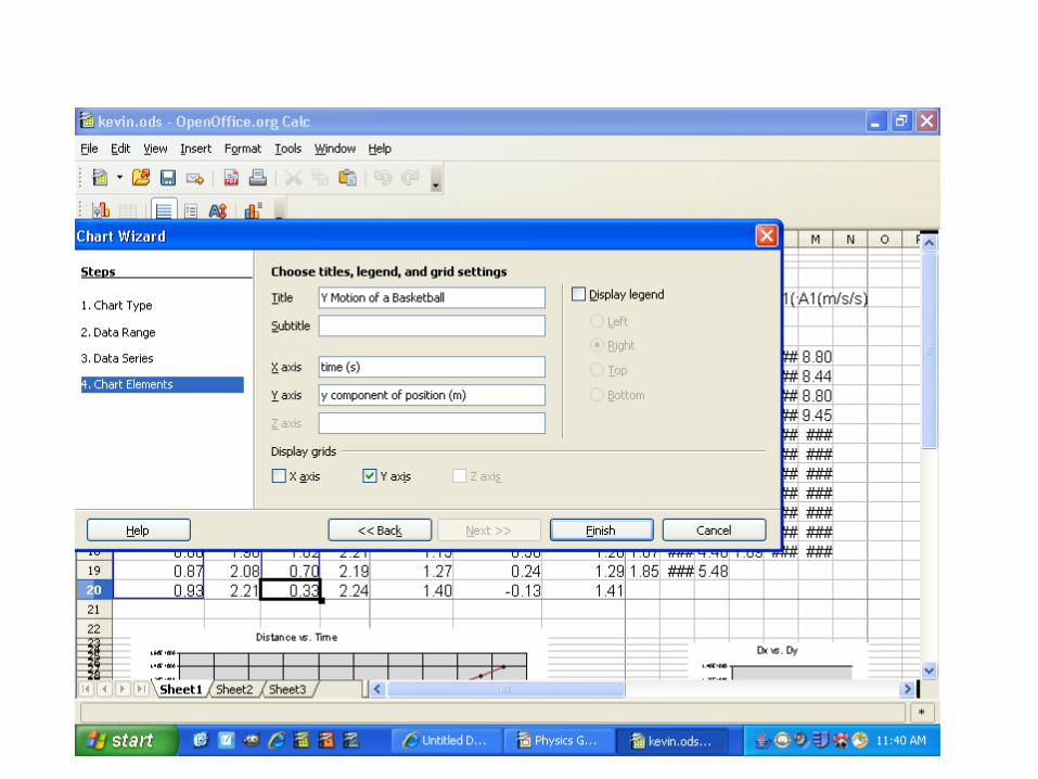
Include a descriptive title, and label each axis. For example, the title Dy vs t is
not descriptive. Be sure to include units.
Unclick the legend.

0 0.1 0.2 0.3 0.4 0.5 0.6 0.7 0.8 0.9 1
0.00
0.20
0.40
0.60
0.80
1.00
1.20
1.40
1.60
1.80

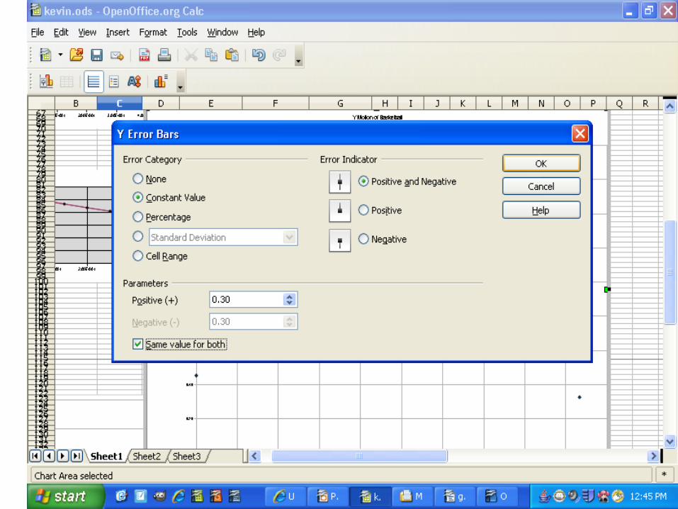
Once you have a graph, click on “insert” then y error bars (no x
bars in Open Office).• Give a value for the y error bars(the
uncertainty). Generally the uncertainty should be half the smallest unit measurable by your measuring device. You may have to calculate the value on the spreadsheet and input using the “cell range” selection.

Click on Insert and trendline.

Choose the correct type of treadline. For linear relationships like F=ma, choose “linear”. For
exponential relationships like d = ½ at2 + Vit choose “exponential”
(Vi = 0) or “polynomial” (Vi non
zero).Note: Non-linear graphs don't seem to work on Open Office.


Double click on the equation and change the font to a reasonable
size.


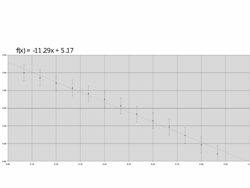
Once you have your equation, you cannot change the format. In
your lab writeup, replace the equation with the correct
variables, units and sig figs.


f(x) = -11.29x + 5.17
Should be replaced with
Vy = -11 m/s2 t + 5 m/s
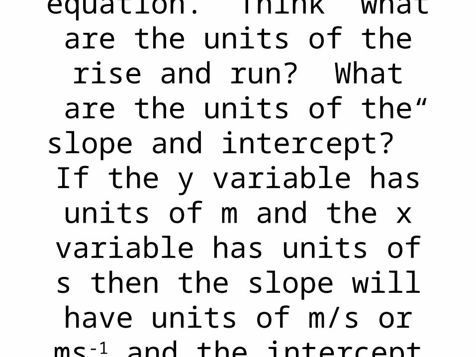
Include units in your equation. Think “what are the units of the rise and run? What are the units of the slope and intercept?” If
the y variable has units of m and the x variable has units of s then the slope will have units of m/s
or ms-1 and the intercept will have units of m.

Check that the graph is clear with the equation easily read. If necessary, resize portions of the graph by moving a corner or side.

Copy the data and calculations into a table in your report.
Display the equations you used (copy and paste them)
0.00 0.10 0.20 0.30 0.40 0.50 0.60 0.70 0.80 0.90 1.00
-6.00
-4.00
-2.00
0.00
2.00
4.00
6.00
f(x) = -11.29x + 5.17
If no labels come with the graph when you paste, put them in.

Vertical Velocity of Basketball
Vy Vy = -11 m/s2 t + 5 m/s
(m/s)
Time (s)
0.00 0.10 0.20 0.30 0.40 0.50 0.60 0.70 0.80 0.90 1.00
-6.00
-4.00
-2.00
0.00
2.00
4.00
6.00

Non-IBers, Done!IBers:
• IB requires that you determine the uncertainty in your graph using max-min lines. You can do this on the computer by just hand drawing two lines on your graph using the drawing tools or a pen.

Vertical Velocity of Basketball
Vy Vy = -11 m/s2 t + 5 m/s
(m/s)
Time (s)
0.00 0.10 0.20 0.30 0.40 0.50 0.60 0.70 0.80 0.90 1.00
-6.00
-4.00
-2.00
0.00
2.00
4.00
6.00

IBers
Calculate the slope of the two lines by hand and half the difference is your uncertainty.
Remeber, uncertainty is to one digit only and the value is rounded to the precision of the uncertainty.
11.1 +/- 2.1 BAD 11 +/- 2 GOOD

Vertical Velocity of Basketball
Vy Vy = (-11+/- 2) m/s2 t + (5+/-1) m/s
(m/s)
Time (s)
0.00 0.10 0.20 0.30 0.40 0.50 0.60 0.70 0.80 0.90 1.00
-6.00
-4.00
-2.00
0.00
2.00
4.00
6.00

You are finished the graph!Does the graph match your hypothesis? Compare the
deviation from theory to the uncertainty. What would account
for the observed relationship? How could you improve the
experiment?