Name ________________________________ Section _______

208R-­‐1C   1  

Physics 208 Laboratory

Interference and Diffraction Your TA will use this sheet to score your lab. It is to be turned in at the end of lab. You must use complete sentences and clearly explain your reasoning to receive full credit. What are we doing this time?

You will complete three related investigations. PART A:

Use a laser and narrow slits to produce multiple coherent light sources that demonstrate interference.

PART B: Determine the track spacing on a CD and DVD using diffraction.

PART C: Investigate thin-film interference by observing dichroic “art glass” and a multilayer plastic bow.

Why are we doing this?

Interference and diffraction are observed wherever there are waves. For instance sound waves, water waves, and light waves all show interference effects. In fact, the colors seen in some birds and insects are not from pigments, but from light interference generated by small-scale structures on their feathers/scales. What should I be thinking about before I start this lab?

You should be thinking about waves, and how the phase difference between waves causes constructive and destructive interference. Any safety issues?

The light source is a laser diode, with a wavelength of about 650 nm. Carefully read the laser handling precautions in the lab manual: the laser diode is a source of extremely intense light, which can damage your or someone else’s vision if mishandled.

When diffracting from the replica grating, CD, and DVD, the diffracted beams can go in unexpected directions. Make sure you aren’t beaming somebody in the eye!

2   208R-­‐1C  

Part A. Interference (This is similar to Experiment II in the lab manual) Here you will be investigating two-slit interference. The two slits illuminated by the

laser beam act as two sources of spherical waves of light that are of the same frequency and same phase. These spherical waves form an interference pattern throughout all space. That is, at all points in space, the total light is a superposition of light originating from the two slits. You investigate the interference pattern visually by looking at the reflection from a white screen, and you record quantitative information on the computer with a light detector that you move manually across the interference pattern.

Your equipment consists of: 1) A laser diode light source, 2) A circular wheel of single slits of various widths, 3) A circular wheel of double slits of various widths and spacings, as well as 4) A diffraction grating mounted to a holder that fits on the optical track 5) A light detector. The light detector also has a circular wheel in front of it, with

apertures of various larger widths. You move the light detector perpendicular to the beam path to quantitatively measure intensity variations of the interfering or diffracted light. The different slits set the spatial resolution of the light detector: slit #2 works well, with a sensitivity setting of “10” (slide switch on detector). If this is too sensitive (so that the detector saturates, as evidenced by flat tops to the diffraction peaks), you can use “1”. If it isn’t sensitive enough, use “100”.

6) A “beam block”. This is an aperture mounted to a holder that fits on the optical track. It is used to block reflections.

7) An optical track on which all these pieces can be mounted. Setup: Position the “Multiple slit set” circular wheel at 110 cm on the track, and

the laser diode directly behind it (this barely fits on the track). Make sure that the circular wheel itself lines up with the 110 cm mark, and not just some part of the plastic holder. This sets the slit-screen distance to 100 cm.

Turn the multiple slit wheel to position the “a=0.04 mm, d=0.25 mm” double slit in front of the laser beam.

Position the detector aperture (labeled “1” or “2” on the aperture wheel) near the center of the track.

If the diffraction pattern doesn’t fall on the detector aperture, use the thumbscrews on the back of the laser to adjust its angle

Put the white screen on the track in front of the light detector.

208R-­‐1C   3  

A1) Describe or sketch what you see on the white screen. A2) The wavelength of the diode laser is about 650 nm. Calculate approximately how many wavelengths of laser light are in the space between the slits and the white screen. A3) Now take off the white screen, and point your lab computer browser to the Physics 208 course web site. Navigate to the laboratories page, and click on the Lab 1 settings file to download it and start the data acquisition program. Use the computer to record the intensity pattern: click start and slowly move the photodetector across the interference pattern by turning the wheel with your hand. Enlarge the data on the computer so only the central peak and two peaks on either side fill the screen. Record the separation between the central maximum and the immediately adjacent minimum, and the next maximum.

From central peak to nearest minimum From central peak to neighbor peak

4   208R-­‐1C  

A4) Here is a sketch of your experimental setup, but not to scale. The slit spacing d is much smaller than shown, and the screen distance L is much larger than shown. The two slits act as two in-phase sources of light. The waves travel out in all directions, and hit the screen in all places – the lines are just to indicate the path of the light that hits the detector at point x.

We showed in class that one path is longer than the other by an amount

€

δ = d sinθ , as long as

€

L >> d . Here θ is the angle of the detector away from the dashed centerline. Using this relation, find the path length difference for the maximum and minimum in

the previous question. (Hint:

€

tanθ = x /L) 1st minimum Next maximum

θ

δ in millimeters

δ in nanometers

δ in wavelengths of laser light

A5) The waves from each slit start out in phase, but they propagate different distances to reach the detector. What is the condition on δ that they Interfere constructively? Interfere destructively?

d

L

Detector

Slits

x

€

δ = d sinθ = path length difference

208R-­‐1C   5  

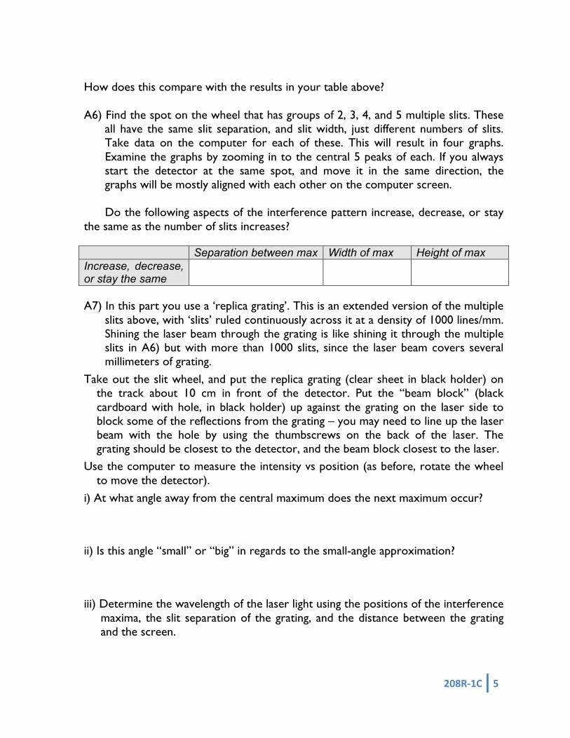
How does this compare with the results in your table above? A6) Find the spot on the wheel that has groups of 2, 3, 4, and 5 multiple slits. These

all have the same slit separation, and slit width, just different numbers of slits. Take data on the computer for each of these. This will result in four graphs. Examine the graphs by zooming in to the central 5 peaks of each. If you always start the detector at the same spot, and move it in the same direction, the graphs will be mostly aligned with each other on the computer screen.

Do the following aspects of the interference pattern increase, decrease, or stay

the same as the number of slits increases? Separation between max Width of max Height of max Increase, decrease, or stay the same

A7) In this part you use a ‘replica grating’. This is an extended version of the multiple

slits above, with ‘slits’ ruled continuously across it at a density of 1000 lines/mm. Shining the laser beam through the grating is like shining it through the multiple slits in A6) but with more than 1000 slits, since the laser beam covers several millimeters of grating.

Take out the slit wheel, and put the replica grating (clear sheet in black holder) on the track about 10 cm in front of the detector. Put the “beam block” (black cardboard with hole, in black holder) up against the grating on the laser side to block some of the reflections from the grating – you may need to line up the laser beam with the hole by using the thumbscrews on the back of the laser. The grating should be closest to the detector, and the beam block closest to the laser.

Use the computer to measure the intensity vs position (as before, rotate the wheel to move the detector).

i) At what angle away from the central maximum does the next maximum occur?

ii) Is this angle “small” or “big” in regards to the small-angle approximation?

iii) Determine the wavelength of the laser light using the positions of the interference maxima, the slit separation of the grating, and the distance between the grating and the screen.

6   208R-­‐1C  

B. Interference from a compact disc and digital video disc. CDs and DVDs have information recorded on closely-spaced tracks spiraling around the disc. Neighboring tracks are separated by a fixed distance. These tracks can act like the slits you used above, but in reflection. This is another type of ‘diffraction grating’. In this section you measure the track spacing on a CD and DVD by interference. Put the white barrier in front of the detector and tape the CD to it. The CD tracks should be vertical at the point the beam hits the CD. Be careful where the reflections from the CD end up – don’t hit somebody in the eye! It helps to turn off the laser when you are not using it. Take a blank sheet of paper, and make a hole about 1 cm diameter for the laser to shine through. Position the paper about 10 cm in front of the CD so that the laser shines through and hits the CD. B1) What do you see reflected on the paper? B2) Estimate the track separation on the CD from the pattern on the paper. (Hint: one easy way is to find the distance of the paper from the CD at which the two diffraction spots hit the (long) edges of the paper. Then you know that they are separated by 11 inches, and the distance from central max to a spot is 11 / 2 = 5.5 inches. This works best if the tracks are vertical where the laser beam hits)

Beam

208R-­‐1C   7  

B3) Repeat for the DVD. B4) Look up typical track spacings for a CD and DVD on the web, and compare. B5) Why do you see colors when white light reflects from the CD/DVD?

8   208R-­‐1C  

C. Thin film interference In parts A and B, you saw how the interference of regularly-spaced light sources can result in constructive or destructive interference. In the first part of the lab, each slit in the wheel or diffraction grating became a tiny source of transmitted light. In the second part, highly reflective tracks on a CD or DVD each became a tiny source of reflected light.

In both of these cases, the light sources were arranged regularly along a surface.

But there are many cases where the reflections are arranged through the thickness of the material. A common example is the soap bubble we discussed in lecture, where reflections from the top and bottom surface of the soap film act as two light sources, which interfere at your eye. When white light shines on the film, some wavelengths (colors) of the light will interfere constructively, and some destructively. You see the colors that interfere constructively.

C1) Make a numbered list of the factors that contribute to the phase difference at your eye of the two reflected beams.

nair=1.0

nfilm=1.5

nair=1.0

208R-­‐1C   9  

C2) Make a rough estimate of the thickness in millimeters of the thinnest film like the one above that would appear yellow (

€

λyellow ≈ 570nm ) when illuminated with white light.

C3) A film like the one above is extremely fragile because it is so thin. In the last ten years, companies have developed processes to efficiently produce microlayer plastic films consisting of hundreds of alternating polyester (n=1.8) and acrylic (n=1.5) layers.

This is analogous to a diffraction grating, with a reflection at each interface between layers in the plastic in the same way that the film interference on the previous page was analogous to two-slit interference.

Here the grating is through the thickness, rather than across the surface as in a CD/DVD.

The Luminesque Fireworks Bow is made from such plastic. Not all tables have these – borrow from another table if you don’t have one. You should at least have some multilayer plastic cut from a lower-quality bow, but it is not as uniform.

You should also have a piece of “dichroic” glass. This glass appears colored because of a multilayer thin-film deposited on its surface.

Look at the bow/glass in three different ways and describe what you see:

i) Hold the bow in front of a window (best) or other light source, and look through the front of the bow at the light source

ii) Continue to look through the bow at the light source. Tilt the bow in various ways, continuing to look at the transmitted light.

iii) Look at the light reflected from the bow.

10   208R-­‐1C  

C4). The figure below is a drawing of a multilayer plastic film as if it had only two layers rather than hundreds. Sketch four different paths the light could take to reach your eye in transmission.

C5) Choose two of the paths, and write down the phase difference between them. Do this in terms of one or both of the layer thicknesses tpolysester and tacrylic and one or both of the indices of refraction.

What layer thicknesses are required to give constructive interference for the observed wavelength (~450nm).

C6) What is one reason that the transmitted color might change when the bow is tilted?

Polyester (n=1.8)

Acrylic (n=1.5)

White light

Air (n=1)

Air (n=1)

Name _________________________________ Section ________

208R-­‐2C   1  

Physics 208 Laboratory

Lenses and the eye

Your TA will use this sheet to score your lab. It is to be turned in at the end of lab. You must use complete sentences and clearly explain your reasoning to receive full credit.

What are we doing this time?

You will complete three related investigations. PART A:

Use a single lens on the optical track to understand what it means to be “in focus”, the lens equation, and the difference between real and virtual images.

PART B: Build a microscope and a telescope on the optical track to understand how the image formed by the objective lens acts as an object for the eyepiece lens.

PART C: Investigate near-sightedness and far-sightedness using an eye model filled with water.

Why are we doing this?

The way lenses use refraction to bend and reform light rays to make an image has myriads of applications. Understanding this will help you get the most out of research instruments such as microscopes.

What should I be thinking about before I start this lab?

You should be thinking about images produced by lenses, and how either a real image or virtual image can act as an object for another lens, such as the one in your eye.

Any safety issues?

The light sources get a bit hot.

2   208R-­‐2C  

A. Lenses Aim your lab computer browser at the course web site laboratories page and click on

the “Virtual Optics Bench” for Lab 1. Click the top button for ‘Converging Lens’, and scroll the page to look at the lens system.

A1. Move the lens around to see the locations at which an image forms on the screen. Then move the screen closer and try again. Is there always the same number of lens positions at which a sharp image forms on the screen? Explain what you found.

Now you will use the Pasco track and light source, the color-coded converging lenses, and a white screen to view images. Position the light source accurately at 0 cm on the track, and the white screen at 30 cm. Put one of the red lenses on the track between the screen and the light source. A2. Find all the positions of one of the red lenses that give a sharp image on the screen

(there is more than one position, but there may not be four)

Lens position (cm)

Image distance (cm)

Object distance (cm)

Magnification

A3. From the data of A2, use the lens equation to calculate the red lens focal length.

208R-­‐2C   3  

B. Microscopes and Telescopes This section involves two-lens systems. These will make a lot more sense if you remember these things: 1. The first lens (objective) forms a real image. 2. The image formed by the objective is used as the object for the (eyepiece) lens 3. A real image will appear on a screen placed at the image location. A virtual image will

not, but your eye can focus the rays from a virtual image on your retina. Compound Microscope Go back to the “Virtual Optics Bench” from the course web site and click the

“Microscope” button. Move the objective with respect to the object and watch the image locations change. After moving them, scroll up and click the “Microscope” button to reset the lens locations to their standard microscope positions.

B1. How does the position of the image formed by the objective move when you change the objective position?

B2. Is the image formed by the objective real or virtual?

.

B3. How does the position of the image formed by the eyepiece move when you change the objective position?

B4. Does the eyepiece form a real or virtual image?

B5. Why does changing the distance between the objective and the object (moving the stage in a microscope) focus the microscope?

4   208R-­‐2C  

Now use the two red lenses to make a compound microscope, an instrument that makes a nearby sample appear larger. Use the light source on the track as a sample.

The objective (lens closest to sample) is used to make a larger, real image of the sample. The eyepiece (lens closest to your eye) is used as a magnifying glass to look more

closely at the image from the objective. B6. Use one of the red lenses as the microscope objective to form an image of the light

source on your white screen somewhere on the track. It is best to not make this first image too big – otherwise the microscope is difficult to set up. Measure the positions of the objective and image and fill in the following table:

Distance of objective from light source Distance of image from objective

B7. Approximately at what location on the track should you position the other red

lens (as the eyepiece) so that you can look through the eyepiece and see a magnified image of the light source? You use the eyepiece as a simple magnifier, whose object is the image formed by the objective.

B8. Complete your microscope by putting the eyepiece at the approximate location,

then moving the eyepiece slightly until you see a magnified image of the light source when you look through the eyepiece with your eye.

Objective lens location: Eyepiece lens location: B9. Now use the 125mm focal length lens (look on the bottom of the lens holder) for

the eyepiece. Objective lens location: Eyepiece lens location Looking through the eyepiece, how is this microscope different than the previous one?

208R-­‐2C   5  

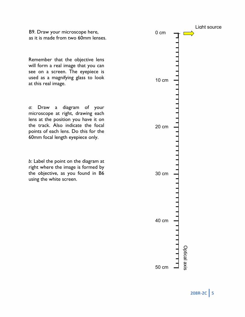
B9. Draw your microscope here, as it is made from two 60mm lenses. Remember that the objective lens will form a real image that you can see on a screen. The eyepiece is used as a magnifying glass to look at this real image. a: Draw a diagram of your microscope at right, drawing each lens at the position you have it on the track. Also indicate the focal points of each lens. Do this for the 60mm focal length eyepiece only. b: Label the point on the diagram at right where the image is formed by the objective, as you found in B6 using the white screen.

Optical axis

Light source 0 cm

10 cm

20 cm

30 cm

40 cm

50 cm

4 5 6 7 8 9 10 11

Data 1

B

6   208R-­‐2C  

Telescope A telescope is an optical instrument that uses two lenses to make a distant object appear closer. The objective lens points toward the distant object (such as the building across the street) and forms an image on the opposite side of the objective lens. The eyepiece is used as a simple magnifier to look more closely at this image.

Go back to the “Virtual Optics Bench” from the course web site and click the “Telescope” button. Change the location of the eyepiece and watch how the image locations change in order to answer the following question.

B10. A telescope is focused by changing the position of the eyepiece. Explain why this works.

Now build a telescope using a green lens (200mm focal length) and a red lens (60mm

focal length. Remove the light source from your track, and arrange the lenses on the track to make a telescope. The telescope is used to view objects far away, so aim the telescope out the window, or at a light board at the other end of the lab room. (You can prop up one end of the track on the eye-model light source)

B11. Use the green lens as the telescope objective to form an image of the distant object on your white screen somewhere on the track.

What is the distance of the image from the objective? B12. At what location should you position the red lens (as the eyepiece) so that you can

look through the eyepiece and see a magnified image of the distant object? B13. Complete your telescope by putting the eyepiece at the appropriate location and

look at various objects.

B14. Now use the orange lens (500mm focal length lens) for the objective, with red lens

as the eyepiece. Look again – how is the telescope different?

208R-­‐2C   7  

C. The eye Your eye also has multiple “lenses”, although they are referred to as the “cornea” and the “crystalline lens”. Both of them do some refracting – these are two closely-spaced lenses. If you wear eyeglasses, that is a third lens! Here is a diagram of your apparatus – it should be full of distilled water to model the vitreous humor.

Rh, R, and Rm are three positions for the retina, letting you model far-sighted, normal,

and near-sighted eyes. C is the cornea – this separates the fluid-filled eye interior from the outside. L is the crystalline lens – in a real eye its focal length by be adjusted by the ciliary

muscle. In your eye model, you adjust the focal length by replacing with different lenses from your box of lenses.

S1 and S2 are locations at which you can add lenses modeling corrective glasses.

You will use four lenses from your lens box: Converging spherical strength +7 diopters Converging spherical strength +20 diopters Converging spherical strength +2 diopters Diverging spherical strength -1.75 diopters

The image formed by the cornea is used as an object for the crystalline lens, just as in the microscope and telescope. But because the lenses are closely spaced, the image formed by the cornea is on the other side of the crystalline lens (the same side as the image formed by the crystalline lens). This means that when the crystalline lens uses this image formed by the cornea as its object, the object distance entered in the lens equation will be negative, since it is on the same side as the real image.

8   208R-­‐2C  

C1. ACCOMMODATION: With the retina in the normal position, point the eye model at a window or other bright object 4 to 5 meters away. Insert the +7 diopter lens in the water at the inside mount farthest from the cornea. An image of the bright object should be in focus on the retina. Next use as object the lamp box and place it about 30 cm from the cornea. The image is blurry until you replace the +7 diopter lens by the +20 diopter lens. This change illustrates accommodation. Eye muscles make the lens thicker for close vision. a) What are the focal lengths in air of the two lenses you used? (The power in diopters is stamped on the lens holders) b) How are the focal lengths of these lenses different when in water in the eye model (are they longer or shorter than for the lens in air?). Explain

c) Both the cornea and eye lens refract the rays to produce an image on the retina. But it can be easier to talk about this pair as a single lens with an ‘effective’ focal length (just as multi-element camera lens are labeled with a focal length). Assuming that this lens is halfway between the cornea and eye lens, what range of focal length was necessary to focus on objects at infinity and at 30 cm? This is the eye range of accommodation.

208R-­‐2C   9  

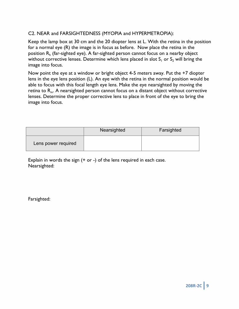
C2. NEAR and FARSIGHTEDNESS (MYOPIA and HYPERMETROPIA):

Keep the lamp box at 30 cm and the 20 diopter lens at L. With the retina in the position for a normal eye (R) the image is in focus as before. Now place the retina in the position Rh (far-sighted eye). A far-sighted person cannot focus on a nearby object without corrective lenses. Determine which lens placed in slot S1 or S2 will bring the image into focus.

Now point the eye at a window or bright object 4-5 meters away. Put the +7 diopter lens in the eye lens position (L). An eye with the retina in the normal position would be able to focus with this focal length eye lens. Make the eye nearsighted by moving the retina to Rm. A nearsighted person cannot focus on a distant object without corrective lenses. Determine the proper corrective lens to place in front of the eye to bring the image into focus.

Nearsighted Farsighted

Lens power required

Explain in words the sign (+ or -) of the lens required in each case. Nearsighted: Farsighted:

10   208R-­‐2C  

C3. Cataracts: A cataract is a cloudy crystalline lens, which usually requires surgical removal. Once the lens is removed, light rays are bent only by the cornea, which alone does not have enough refracting power to form a sharp image on the retina.

Put the retina back in the middle (normal vision) position, and carefully remove the eye

lens using your best surgical technique. Verify that without the eye lens a sharp image never forms on the retina, regardless of the light source location. Historically the eye lens was not replaced, and eyeglasses were used to provide the additional focusing power. In this case it is important to determine the focusing power (hence focal length) of the cornea alone.

a. Put in the +7 diopter lens (outside the eye, as glasses) and adjust the light source

distance so that a sharp image is formed on the retina. Draw your setup below, indicating positions of the object, image, eyeglass lens, and cornea.

Name________________________________________ Section___________

208R-­‐4C   1  

Physics 208 Laboratory Electric Fields and Electric Potentials

Your TA will use this sheet to score your lab. It is to be turned in at the end of lab. You must use complete sentences and clearly explain your reasoning to receive full credit.

What are we doing this time?

You will complete two related investigations. PART A:

Use a numerical simulation to plot on the screen equipotentials and electric field vectors various charge distributions, and see how the presence of additional neutral conductors .

PART B: Use the field plotting board to map the equipotentials of a dipole, and to determine how the potential difference ‘across’ a dipole depends on the angle with respect to the dipole axis.

PART C: Use the field-plotting board and the torso cutout to understand how an electrocardiogram measures properties of the heart electric dipole.

Why are we doing this?

To understand the electric potential energy around charges and conducting objects, and how to apply this understanding to interpreting an electrocardiogram

What should I be thinking about before I start this lab?

You should be thinking about the relation between electric potential, work, and energy.

Any safety issues?

No

2   208R-­‐4C  

A. Numerical Simulation Click on “EM Simulator” in the applets column on the course web site

“Laboratories” page. The electric field at each point is shown as a vector, but all the vectors have the same length: the magnitude of the electric field is indicated by color. White = large electric field Light Green = medium electric field Dark Green = small electric field You should be able to click and drag the positive charge around on the screen.

A1. The white line contours are equipotentials, connecting

points in space that have the same electric potential. Each contour is a different electric potential, and the electric potential difference between adjacent contours is a constant value ΔV.

Why do the equipotentials get farther apart as you move away from the charge? (Answer in terms of the relation between electric field and electric potential).

A2. Conducting Planes Under the setup menu choose ‘Conducting Planes’. Two plates appear, with equal and opposite electric potential. Move the plates around with your mouse to see the effects on the field lines and equipotentials.

When the plates are aligned, the equipotential lines are approximately equally-spaced between them. Explain why this is so.

208R-­‐4C   3  

Yellow indicates positive charge, and blue indicates negative charge. Explain how the

charge arrangement is consistent with the direction of the electric field between the plates.

Explain how the relative magnitude of the electric fields between the plates and outside

of the plates is consistent with the charge distribution. A3. Move the plates to the top and bottom of the screen. Select “Mouse=Add Conductor (Gnd)” from the Mouse

dropdown menu. Draw an empty box as indicated. Select “Mouse=Make Floater” and convert the grounded

conductor to a floating conductor by putting your mouse over it and clicking. It is now an isolated conductor with zero net charge.

Explain why the charge is distributed as it is on the box

that you drew. Select “Mouse=Move Object” from the Mouse dropdown menu, and move your box

around the screen. What is the electric field inside the box?

4   208R-­‐4C  

A4. Dipole and induced charges Under the setup menu choose ‘Dipole’. You should see +

and – point charges with the corresponding field lines and equipotentials.

Click and drag the charges so that the dipole is horizontal near the bottom of the screen, and takes up most of the screen.

Select ‘Mouse=Add Conductor (Gnd)’ and draw a filled rectangle near the top of the screen.

Select ‘Mouse=Make Floater’ and convert the grounded conductor to a floating conductor by putting your mouse over it and clicking. It is now an isolated conductor with zero net charge.

Select ‘Mouse=Move Object’ and drag the conductor around on the screen. The local charge density on the conductor is color coded, blue for negative and yellow for positive.

i) Drag the conductor down near or

between the dipole charges. Describe what happens to the charge distribution on the conductor, and how the electric fields change. What value do you think the electric field has inside the conductor? Explain what is going on.

ii) How can the presence of the conducting object affect the fields near the dipole? (Hint: how would you describe the induced charge distribution on the conducting

object, and how would this effect the fields? )

208R-­‐4C   5  

iii) Suppose the dipole is an electrogenic fish, i.e. a fish that can cause a charge separation in its own body between its head and tail. Suppose that the conducting object is its (conducting) prey. The electrogenic fish senses its prey by detecting changes in electric fields on its own skin caused by the conducting prey. Move the prey around and watch the electric fields in the region of the dipole.

What do you think are some of the factors that affect how close the conductor must

be to the fish before it noticeably affects the electric fields at the fish?

6   208R-­‐4C  

B: Analog simulation Here you use a piece of carbonized paper in which currents flow to simulate

electric fields and equipotential surfaces in vacuum. B1. Electric equipotential lines of an electric dipole. Field plotting board: Get a piece of graphite paper with two silver dots (representing

conducting spheres), one on each end. On the field plotting board, first put down a sheet of white printer paper, then a sheet of carbon paper (carbon side down), and finally the graphite paper on top.

Power supply: Use a red banana-plug cable to attach the +30V output (red) of the DC power supply to one magnet connector on the field plotting board, and a black cable to attach the ground output (black) to the other. Put the magnet connectors on top of the silver dots on the graphite paper. This maintains a constant potential difference between the two painted conductors on the graphite sheet.

Digital multimeter: Attach the red and black voltage probes to the Keithley digital multimeter (DMM) by attaching a BNC to banana-plug adaptor to each probe. Then connect a banana plug cable from the red probe to the DMM red connnection, and from the black probe to the DMM black connection. Sit one probe in each of the field plotting board electrical connections. Turn the multimeter on. The multimeter can measure multiple quantities (voltage, resistance, or current), so you have to tell it to measure voltage by pushing the ‘V’ button. Put it on the ‘automatic’ scale of the DC voltage measuring function by pushing the ‘Auto’ button.

Adjustments: Turn on the DC power supply and adjust the voltage until the multimeter reads about 20V (the switch just above the connections should be on ‘30V’ and not ‘1000V’). The display on the multimeter is the electric potential difference across its inputs, VRed – VBlack.

Voltage  supply  

208R-­‐4C   7  

B1. Electric equipotentials of a dipole:

You should have a graphite sheet with two silver dots representing different charges on a dipole. Rest the black probe from the voltmeter in the banana plug connected to the voltage supply black terminal. Map out equipotential lines using this procedure: 1) Pick a number between 0 and 20, and write it down (you’ll need it later). 2) Probe around with the red probe until you read that number on the DMM 3) Push down firmly with the red probe at that spot. This will cause some of the carbon

on the carbon paper to transfer to the white paper underneath. 4) Probe around and find another spot with the same potential. Push down firmly to

make another dot. Do this enough times so that later you will be able to connect the dots with a line that you can label with a numerical value for the potential.

6) This is an equipotential: a connected set of points with the same electric potential. 7) Pick another number and repeat. 8) When you have enough lines to make a nice picture, take off the graphite and carbon

paper, and connect the dots. You should have at least four lines. Draw your equipotential lines below, and label each with their potential:

20V 0V

8   208R-­‐4C  

B2. Electric potential differences around a dipole Now put the dipole back on the field plotting board (you won’t need the carbon paper or the white printer paper). Connect the banana plugs from the + and – terminals of the power supply to the silver dots on the graphite paper. Now pick up the red and black voltage probes connected to the voltmeter, one in each hand. Put the probes a fixed distance apart on the graphite paper at various angles with respect to the dipole axis as shown below, and read the voltage from the multimeter.

Record your data here for the given angles : Angle 30 45 60 90 120 135 150 VA - VB

Plot your results here. You will use this in interpreting the ECG in the next section. On the same plot above, draw in points based on your equipotentials of part B1. Comment below on similarities / differences.

Dipole axis

0V 20V

VB(90˚)

VA(90˚) VA (45˚)

VB (45˚)

VA (30˚)

VB (30˚)

VB(120˚)

VA(120˚)

ANGLE (DEGREES)

POTENTIAL DIFFERENCE ( V )

90˚ 180˚ 135˚ 45˚ 0˚

208R-­‐4C   9  

C. Electrocardiagrams and dipoles In this section you use the conducting sheet and the computer to make an electrocardiogram measurement.

Your heart is embedded in a conducting medium (your body), and is electrically active. This causes currents to flow in your body, and electric potentials develop throughout your body. An electrocardiogram measures potential differences at various points on the surface of your body, and tries to figure out what is happening at your heart. In this section you set up an electrical signal inside the conducting sheet, and investigate the dipole magnitude and direction by looking at potential differences on the outside. This is similar to the way an electrocardiogram obtains information about your heart. In a common approximation, the electrical activity of your heart can be characterized as an electric dipole, with a potential difference between the two poles. The electrocardiogram is trying to determine the orientation of a dipole in your heart by making measurements on the surface of your body.

How can a heart be a “dipole”? When your heart beats, it establishes a very complicated charge and potential distribution that changes in time as different parts of the heart are stimulated. Your heart accomplishes this by moving around positive and negative charge.

The total charge is always zero, just rearranged, so a dipole is a good approximation. The ‘fine-tuning’ charge distribution that differentiates the actual distribution from a dipole is not very important. It generates a potential that dies away rapidly as you move away from the heart. So from far enough away, the potentials in the body due to the heart are indistinguishable from those produced by a dipole.

Here is a picture of the heart dipole at an instant 240 ms into a heartbeat, and a plot showing the tip of the dipole vector as a function of time (dotted path). The heart dipole changes both direction and magnitude during the heartbeat.

px

Py

10   208R-­‐4C  

Remove the dipole graphite sheet and carbon paper, and substute the torso cutout (no carbon paper) as shown. The three main leads of an electrocardiogram are usually called Lead I, Lead II, and Lead III. These all give different views of the heart dipole. In terms of the electric potentials VRightArm (VRA), VLeftArm (VLA), and VLeftLeg (VLL), the voltages mesured by the three leads are: Lead I measures ______________

Lead II measures ______________

Lead III measures ______________

Download the settings file from the “Laboratories” page of the Physics 208 course web site. This opens the data acquisition program with the correct settings. You will use the large magnet electrodes to connect the leads to the arm and leg Input A of the Pasco interface for Lead I Input B of the Pasco interface for Lead II Input C of the Pasco interface for Lead III You will use the small magnet electrodes to connect the 30V output of the DC power supply to two of the heart dipole connections. Connect a banana plug cable from the red and black 30V connections to the heart dipole magnet electrodes to power your heart model.

VLA  

VLL  VRA  

208R-­‐4C   11  

Set the voltage supply to 10V. The heart now has an electric dipole moment, and each of the three leads will measure some electric potential difference. We will refer to these voltage signals as “resting voltage”.

You will change the heart electric dipole moment, to simulate the heart beat, by turning the knob on the power supply to increase and decrease the applied voltage.

Click ‘start’ on the data acquisition program, and use the knob on the voltage supply to increase the voltage to 20 or 25 volts, down below 10V, then back up to 10V, to simulate a heartbeat (ba-bump!). If you do this quickly, then wait a second, and then repeat, etc, it will look more like a heartbeat on an electrocardiogram.

Then move the small magnet electrodes to the other (perpendicular) pair of dots, and take another set of ECGs. C1) For your two different orientations of the heart dipole, measure the excursion

(positive or negative) from the resting voltage for leads I, II, and III. The resting voltage is the value of the signal with the voltage set at 10V, in between heartbeats.

Orientation Lead I Lead II Lead III

#1

#2

To generate this data, you used a fixed heart dipole direction, and varied the magnitude of the dipole by turning the knob on the power supply to simulate the heartbeat. You also used a different dipole direction (~ perpendicular to the first one) that gave a very different set of ECG traces.

This different dipole direction might indicate a heart problem. For instance, if part of the heart is enlarged, the extra tissue in that part leads to a bigger component of the dipole in that direction.

12   208R-­‐4C  

You obviously know the dipole directions you used for the two different data sets. But suppose you didn’t know, and you needed to use the ECG traces to determine the dipole direction and magnitude (pretend you are a cardiologist). For each of your data sets, use your work in part B2) to qualitatively determine the direction of the heart dipole. Print out your ECGs if it is easier for you to analyze them that way. C2) Explain below how you used the ECG data to determine the dipole direction. Here

are some questions to help you think about the problem.

Suppose one of the ECG leads gives a very small signal. How can you tell if this is because the dipole has a small magnitude, or because it has a particular orientation? Suppose two ECG leads give almost the same voltage signal. What does this mean about their orientation relative to the dipole? Suppose two ECG leads have the opposite sign of signal. How must the dipole be oriented?

Name _______________________________ Section ___________

208R-­‐5   1  

Physics 208 Laboratory Capacitor circuits and resistor circuits

Your TA will use this sheet to score your lab. It is to be turned in at the end of lab. You must use complete sentences and clearly explain your reasoning to receive full credit. What are we doing this time?

You will complete three related investigations. PART A:

Build capacitor circuits, investigating charge distributions and voltages. PART B:

Build a circuit with light bulbs, using the relative brightness of the bulbs to visualize the current flow.

PART C: Build resistor circuits, and measure current and voltage. Why are we doing this?

Capacitors are almost as ubiquitous as dipoles, showing up almost everywhere there is an insulator. Actually, capacitors have some similarities to dipoles, with equal and opposite charges on the electrodes. That charge has to flow through something to get to the capacitor. The same holds for resistors. The ideas of current flow, current splitting along different paths, and potential differences, are essential ideas in all circuits. What should I be thinking about before I start this lab?

You should be thinking about the aspects of capacitors you looked at in lecture and discussion. In particular, how the voltage across the capacitor is related to the charge on it, and how the current in a circuit delivers charge to a capacitor. Also how charge moves in a circuit, and that charge must always be conserved – it can be neither created nor destroyed.

2   208R-­‐5  

For the first part of the lab, you use the circuit board below.

Holes connected by black lines are electrically connected by conducting wires, so all points connected by black lines are at the same electric potential. You build a circuit by plugging in resistors and capacitors across the gap between crosses. The capacitors and resistors are built into plastic blocks with banana-plug connectors that exactly bridge the gaps. After you plug in a block, there will still be unused holes in each cross. You will use the remaining holes to connect the voltage source to supply your circuit with charge, and to connect the electrometer (capacitor circuits) or Keithley Digital Multimeter (resistor circuits) to measure potential differences and currents at various points in the circuit. The voltage source provides a constant voltage of 12 V.

These 5 points connected together

Resistor or capacitor block goes here

208R-­‐5   3  

A. Capacitor circuits. You use the electrometer and the voltage probes to measure voltages. Connect the red probe to the electrometer ‘input’ connection, and the black probe to the electrometer ‘ground’ input with black coaxial cables (not the banana plug cables). You don’t need any adaptors: the coaxial cable connects directly to the probe and to the electrometer.

1) Series capacitors: you will build the circuit below and measure it, but first predict how the 12V provided by the voltage source will split among the two series capacitors. V across C1: V across C2: Build the circuit below (note that the voltage source is not connected). a) First, temporarily short out each capacitor, by plugging it into the metal holder, to

make sure there is no charge separation between the plates. b) Touch the black and red voltage source leads across the series circuit, then

disconnect both the black and red leads from the circuit. c) Use the electrometer to measure the voltage drops across each capacitor

individually with the supply disconnected. Compare these to your prediction.

1.0 µF 0.47 µF

ConstantVoltage Source

C1 C2

4   208R-­‐5  

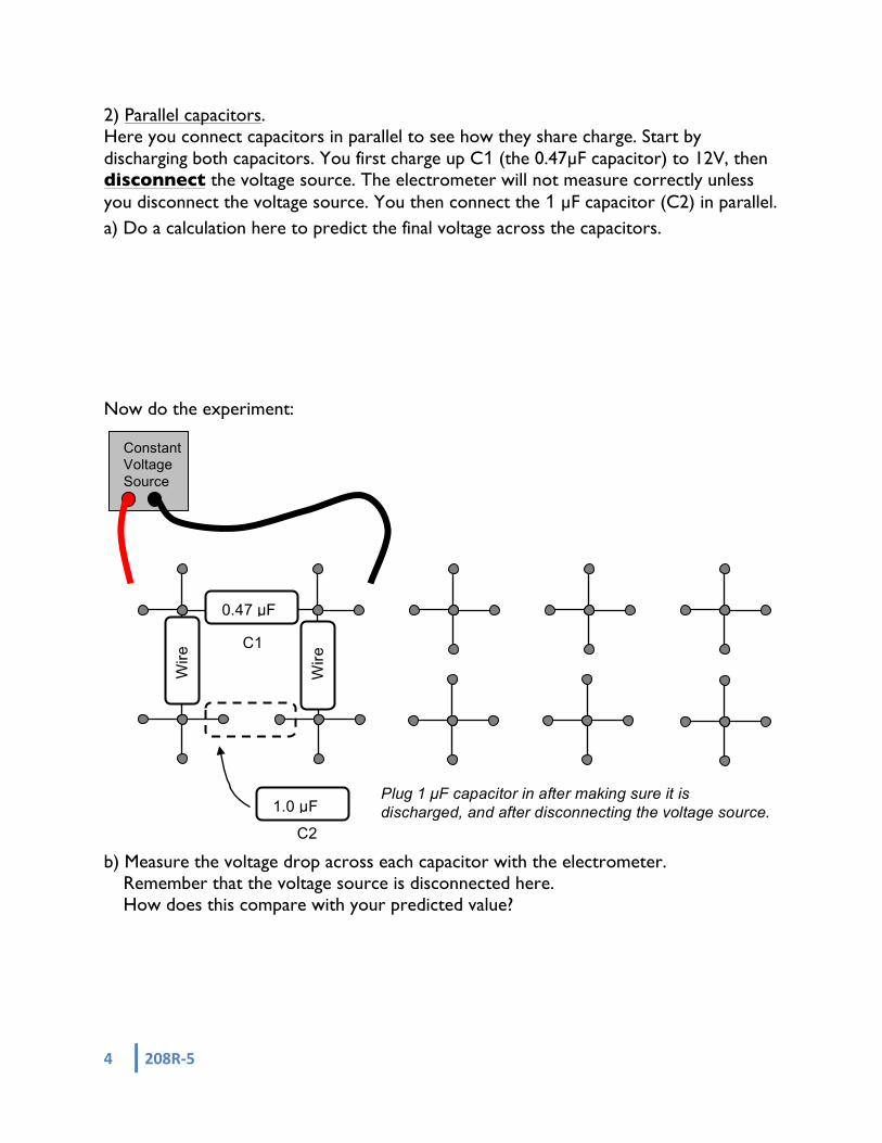
2) Parallel capacitors. Here you connect capacitors in parallel to see how they share charge. Start by discharging both capacitors. You first charge up C1 (the 0.47µF capacitor) to 12V, then disconnect the voltage source. The electrometer will not measure correctly unless you disconnect the voltage source. You then connect the 1 µF capacitor (C2) in parallel. a) Do a calculation here to predict the final voltage across the capacitors. Now do the experiment: b) Measure the voltage drop across each capacitor with the electrometer.

Remember that the voltage source is disconnected here. How does this compare with your predicted value?

C1

C2

Constant Voltage Source

1.0 µF

0.47 µF

Wire

Wire

Plug 1 µF capacitor in after making sure it is discharged, and after disconnecting the voltage source.

208R-­‐5   5  

B. Light Bulbs. Compare the brightness of several combinations of light bulbs. The brightness of the bulb is a good qualitative indication of how much current is flowing through the circuit. A brighter bulb means a larger current. 1 Amp of current represents the movement of 6.242x1018 electrons through the bulb each second. There are three identical incandescent light bulbs at the table. Begin by comparing a single bulb to two in series. Starting with a single bulb, build the following circuit: Next, add a second bulb after the first one, as shown below. Which bulb do you predict will be the brighter of the two?

Now do the experiment. Explain the relative brightnesses of the three bulbs in the above circuits, in terms of the movement of electrons through each bulb:

Which bulb is brighter?

Bulb Wire

Bulb Bulb

1

ConstantVoltage Source Source

2

Constant Voltage Source

Bulb Wire

6   208R-­‐5  

Next, compare the brightness of a single bulb to two bulbs wired in parallel. First, connect one bulb to the voltage source. Then add a second bulb in parallel with the first (see diagram below). Predict how the brightness of the first bulb will change when the second is added:

Now do the experiment.

How did the brightness of the first bulb change when the second was added? How did the voltage provided by the voltage source change when the second bulb was added? How did the current flowing out of the voltage source change when the second bulb was added? How does the current flowing through the first bulb compare to the current flowing through the second bulb? How does the current flowing through either bulb compare to the current that flowed through the single bulb in the first circuit described on the previous page?

Bulb

ConstantVoltage Source

Wire

Wire

Bulb

208R-­‐5   7  

Lastly, compare the brightness of two bulbs combined in series to one bulb connected in series with a pair of bulbs wired in parallel (see diagram below). Predict how the brightness of bulb A will change when the extra bulb is added:

How did the brightness of bulb A change when the extra bulb was added?

Using Ohm’s law, compare the equivalent resistances of the two circuits, with and without the extra bulb. Which has the larger equivalent resistance?

How did the voltage provided by the voltage source change when the extra bulb was added? How did the current flowing out of the voltage source change when the extra bulb was added? How does the current flowing through bulb A compare to the current flowing through the extra bulb?

Bulb Bulb

Constant Voltage Source

Wire

Wire

Bulb

A

8   208R-­‐5  

C. Resistor circuits. 1) Measuring current and voltage. Build the circuit below using first the resistor labeled

10kΩ resistor for R. Then use 20kΩ and 100kΩ.

The digital mulitimeter (DMM) can be configured to measure current, voltage, or resistance. Here you want to measure

current. Press the ‘A’ button for amps, then ‘2m’ for a 2 mA scale. The DMM now acts as an ammeter, and it displays how much current flows through it. In this mode it is very low resistance. So it acts like a connecting wire while measuring current, and doesn’t alter the properties of the circuit. Positive current flowing into the red terminal of the DMM and out of the black terminal gives a positive reading on the display. Which way do the electrons move? How much work is done by the power supply to move one electron around the circuit? Complete the following table. The resistor labels are ‘nominal’ values — the actual resistance is likely to be a little different. These resistors are guaranteed to be within 10% of their labeled value. Resistor Voltage V Current I V / I = Calc. Resistance 10 kΩ 12.0V 20 kΩ 12.0V 100 kΩ 12.0V

Constant Voltage Source

R

Keithley DMM

208R-­‐5   9  

2) Now build the circuit below, and measure the current. Here the ‘wire’ is a plug-in

block that is a metal conductor.

Explain in words whether the measured current will increase, decrease, or stay the same when you remove the 10 kΩ resistor. Then pull it out and see if you were right.

Calculate the value of the current you measured at the top of the page.

C

Constant Voltage Source

20 kΩ

Keithley DMM 10 kΩ

Wire

Wire

Current =

Value Units

10   208R-­‐5  

3) Voltage drops around the circuit, and measuring current with voltage drops. In part 2) you saw that the DMM can measure current directly, but it must be inserted in the path of the current so that current can flow through it. This makes it difficult to quickly probe current in different parts of the circuit.

Press the ‘V’ button on the DMM so that it displays the electric potential difference between its red and black terminals. In this mode, almost no current at all flows through the DMM – it acts like an extremely large resistor while measuring voltage.

Then press the ‘Auto’ button so that it changes scales automatically.

Explain why you use the DMM to measure the current through a resistor by measuring electric potential difference (voltage drop) between the two ends of the resistor. Now make the circuit below: Use the DMM as voltmeter to determine the current through each of the resistors by measuring voltage drops. Write the current below. Current through R1: Current through R2:

ConstantVoltage Source

100 kΩ 10 kΩ

R1 R2

208R-­‐5   11  

In the next step you will put a 20 kΩ resistor (call it R3) in parallel with R2. But before making the circuit, predict whether currents through R1 and R2 will increase or decrease.

Current through R1: Current through R2:

Explain: Now build the circuit below, and determine the voltages and currents.

Voltage across R1: Current through R1: Voltage across R2: Current through R2: Voltage across R3: Current through R3: Voltage across wire block: Current through wire block Explain how this agrees or disagrees with your prediction. Explicitly verify that current is conserved at the node indicated above by showing that the current flowing into the node is the same as the current flowing out.

R3

I1 I2

Constant Voltage Source

100 kΩ 10 kΩ

20 kΩ

Wire

Wire

R1 R2

I3

Show current conservation here

12   208R-­‐5  

This page intentionally blank

Name _______________________________ Section ___________

208R-­‐6C   1  

Physics 208 Laboratory Resistor-Capacitor (RC) Circuits

Your TA will use this sheet to score your lab. It is to be turned in at the end of lab. You must use complete sentences and clearly explain your reasoning to receive full credit. What are we doing this time?

You will complete two related investigations. PART A:

Build resistor-capacitor circuits, and measure time-dependent currents and voltages. PART B:

Use these ideas to measure and investigate a cell membrane electrical model, investigating propagation of an action potential down the cell membrane.

Why are we doing this?

Capacitors are almost as ubiquitous as dipoles, showing up almost everywhere there is an insulator. Actually, capacitors have some similarities to dipoles, with equal and opposite charges on the electrodes. And they almost always show up in combination with some non-insulator — a resistor-capacitor circuit! What should I be thinking about before I start this lab?

You should be thinking about the ideas of circuits you developed when looking at resistors and capacitors last week. In particular, how the voltage across the capacitor is related to the charge on it, and how the current in a circuit delivers charge to a capacitor.

2   208R-­‐6C  

For the first part of the lab, you use the same circuit board as you did last week. The board is shown below:

Holes connected by black lines are electrically connected by conducting wires, so all points connected by black lines are at the same electric potential. You build a circuit by plugging in resistors and capacitors across the gap between crosses. The resistors are built into plastic blocks with banana-plug connectors that exactly bridge the gaps. After you plug in a resistor, there will still be unused holes in each cross. You will use the remaining holes to connect the variable voltage source to supply your circuit with charge, and to connect the Keithley DMM or Pasco interface to measure currents and potential differences at various points in the circuit.

These 5 points connected together

Resistor or capacitor block goes here

208R-­‐6C   3  

A. Resistor-capacitor circuits. Here you connect a resistor and capacitor to investigate how a capacitor charges and

discharges. Turn the DC voltage source on and set it for zero volts output. Connect the DC voltage source and Keithley multimeter to the 10 MΩ resistor and 1 µF capacitor as shown below. Configure the multimeter to measure current by pressing the ‘A’ button, and then the ‘200µ’ to put it on the 200 µA scale.

Quickly increase the voltage on the DC supply to about 20 V and watch the current of the DMM. Wait until the current stabilizes (this could take a long time), then quickly turn the voltage supply to zero volts, and watch the current again. 1) What is the direction of the current after increasing the voltage from 0V to 20V? 2) The current represents a charge flow. What happens to this charge after it goes

through the resistor? 3) What is the direction of the current after decreasing the voltage 20V to 0V?

Remember that when the supply reads zero volts, there is no potential difference between the red and black terminals: it is as if a wire connects them.

10MΩ

1.0 µF

Wire

30V

DC voltage source

1000V

Multimeter

4   208R-­‐6C  

4) How do think the voltage across the capacitor changed as a function of time when you changed the power supply 0-20V? Why?

5) How does the capacitor voltage affect the current through the resistor? (Think

about Kirchoff’s loop law). 6) You saw that the current through the resistor changes smoothly with time. But it can be easier to think about this in short time steps. Calculate values for the following table to approximate the current as a function of time just after you increase the voltage from 0V to 20V. Don’t make experimental measurements here – just use your calculator. ΔQR is the charge that flowed through the resistor during the previous 2 sec. QC is the charge on the capacitor VC is the voltage drop across the capacitor; VR is the voltage drop across the resistor IR is the current through the resistor. IRprev is the current during the previous 2 sec.

Time ΔQR=IRprev

€

Δt QC VC VR IR 0 0 2 sec 4 sec 6 sec 8 sec 10 sec 12 sec 14 sec Using your table above, sketch the voltage across the capacitor as a function of time. 7) Now replace the 10MΩ resistor with a 100KΩ resistor and increase/decrease the supply voltage. How does the behavior compare with that of the 10MΩ circuit?

VC

TIME

208R-­‐6C   5  

Now you use the computer to measure the time-dependent current through the resistor. Use the 1 µF capacitor, and the 100 kΩ resistor. To make an accurate measurement, the voltage needs to be switched very quickly from 0V to 10V (the Pasco can measure only up to 10V), more quickly than you can do it by turning the knob. Set up the circuit below to quickly switch the voltage, with the power supply at 10V. 1) What will be the potential difference between points A and B when the switch is … a) all the way to the right? b) all the way to the left? 2) The Pasco inputs A, B, and C always measure voltage. What voltage does input A measure in this circuit? How can you use this voltage to determine the current flowing through the resistor? Now move the switch all the way to the right. Start the data acquisition program by clicking on the LabSettings1 file on the Laboratory page of the course web site. Click start and measure the time-dependence of the current through the resistor when you flip the switch all the way to the left, then all the way to the right, repeating several times. Your switch may have a center position — we don’t use it.

Switch

A

B

100KΩ

1.0 µF

Wire

Pasco interface A

30V

DC voltage source

1000V

6   208R-­‐6C  

3) What is your measured maximum measured current, and when does it occur? 4) Calculate the expected value of this maximum current, and compare to 3). 5) Directly from the data on the computer, determine the time constant τ of the circuit. 6) Calculate the time constant from the resistor and capacitor values and compare to

your measurement in 4).

7) Your data on the screen is ‘voltage across the resistor’ vs time, which you showed in 2) is proportional to the current vs time. Find the proportionality factor, and explain why the area under this curve times the proportionality factor is equal to the final charge on the capacitor.

8) Use the mouse to select the decay from maximum to zero current on your graph, and find the area under the curve by selecting ‘area’ from the ‘statistics’ ( Σ ) pull-down menu at the top of the graph. Multiply this area by the proportionality factor you found in 7) and enter it in the box below.

Area under curve Value Units

9) Calculate the expected value of this area from how the charge on the capacitor is

related to its electric potential (you don’t have to do any integration). How does your value compare to the measured one?

208R-­‐6C   7  

Now think about this circuit, but don’t build it or measure it. Why would you ever care about this circuit? Be patient — in the next section you use

this as a basis for a model of a nerve signal (action potential) propagating down a cell membrane.

1) Suppose the capacitors start out discharged, and you apply 10V across the circuit.

At the instant you apply the voltage, what are the currents through R1 and R2? 2) Where does the charge flowing at this instant end up? 3) Think about later time intervals. Why does C1 charge up sooner than C2? If the voltage rising above some threshold value across each capacitor triggered

something to happen, then that event would occur sooner at C1 and some time later at C2. In this way you can think about this as a signal propagating down the circuit (e.g. an action potential). In the next section you watch a voltage pulse propagate down a similar circuit.

R1=100 KΩ

C1=1 µF C2=1 µF

R2=100 KΩ

8   208R-­‐6C  

B. Electrical model of a cell membrane F Cell membrane equivalent circuit

As discussed in class, a cell membrane has a potential difference between its interior and exterior. The low-resistance cell exterior is modeled by a low-resistance wire. The medium resistance cell interior is modeled by 100 KΩ resistors. The capacitors model the insulating lipid bilayer. The potential difference arises from charges in the conducting fluids that form the electrodes of the cell-membrane capacitor. These charges move around in the fluids, making the potential difference vary with position. This makes an action potential (generated at the left end) that propagates down the cell membrane.

The switch models an ion channel that is triggered by some external stimulus, mechanical, chemical, or electrical. It could be a channel opening in response to a pinprick in your finger. This causes a change in potential difference at that location.

No other ion channels are modeled here. In a real cell membrane, there are voltage-triggered ion channels distributed throughout. We don’t include them here because these are not simple (

€

V ≠ IR) resistors. For instance, when the potential across the cell membrane reaches a threshold value, the non-Ohmic (

€

V ≠ IR) resistors reduce their resistance to quickly bring it back to its resting state. This makes the action potential a sharp pulse and sustains its amplitude. This also changes the propagation speed from that with Ohmic resistors.

We use a pulse generator to start the pulse, and also to bring the potential back to its resting value. Here only the resistor-capacitor network is modeled, and not the sustaining effect from the non-Ohmic resistors. So the pulse broadens and decays. But still our model is able to capture some aspects of the action potential propagation.

Hodgkin and Huxley shared the 1963 Nobel prize in physiology and medicine partly in recognition of their analysis of the full non-Ohmic electrical circuit model.

Pulse generator

Interior of cell

Exterior of cell

Lipid Bilayer

30V

DC voltage source

1000V

100 KΩ 100 KΩ 100 KΩ 100 KΩ 100 KΩ

WIRE

1 µ

F

1 µ

F

1 µ

F

1 µ

F

1 µ

F

WIRE WIRE WIRE WIRE

A1

B1

A2

B2

A3

B3

A4

B4

A5

B5

A6

B6

208R-­‐6C   9  

To start the action potential, you will (in the next section) introduce a voltage pulse at A1,B1, and watch it propagate down the cell membrane, similar to an action potential.

If you could measure all the potential differences Ai,Bi at two different instants in time (t1 [squares] and t2 [triangles]), you might see something like the following.

You can only measure potential differences across the capacitors – the squares and

triangles represent potential differences measured at these locations. The dashed line is what the voltage pulse might look like in an actual, continuous, cell membrane. The triangles correspond to the voltage differences at slightly later time ( t2 ) than the squares ( t1 ). This data indicates that the voltage pulse is traveling to the right at some speed, since the peak voltage position has moved.

You won’t be measuring the voltages across all the capacitors simultaneously

because there are not enough computer inputs. You will measure the voltage across each capacitor separately as a function of time. For instance, at position 2, the voltage is large at time t1 and then smaller at time t2. The voltage at position 3 is small at time t1, and has gotten larger at time t2.

Your job will be to record the voltage vs time for each capacitor in the membrane, and then reconstruct a graph like the figure above that shows a snapshot of the voltage pulse at different times as it propagates down the cell membrane.

SPATIAL POSITION

PO

TEN

TIA

L D

IFF.

( V

)

Cap. 1 Cap. 2 Cap. 3 Cap. 4 Cap. 5

Time t1

Time t2

10   208R-­‐6C  

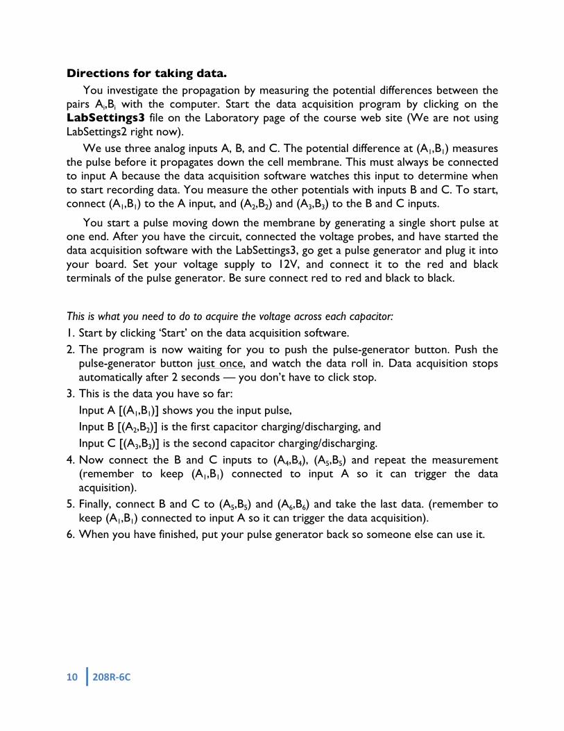
Directions for taking data. You investigate the propagation by measuring the potential differences between the

pairs Ai,Bi with the computer. Start the data acquisition program by clicking on the LabSettings3 file on the Laboratory page of the course web site (We are not using LabSettings2 right now).

We use three analog inputs A, B, and C. The potential difference at (A1,B1) measures the pulse before it propagates down the cell membrane. This must always be connected to input A because the data acquisition software watches this input to determine when to start recording data. You measure the other potentials with inputs B and C. To start, connect (A1,B1) to the A input, and (A2,B2) and (A3,B3) to the B and C inputs.

You start a pulse moving down the membrane by generating a single short pulse at one end. After you have the circuit, connected the voltage probes, and have started the data acquisition software with the LabSettings3, go get a pulse generator and plug it into your board. Set your voltage supply to 12V, and connect it to the red and black terminals of the pulse generator. Be sure connect red to red and black to black.

This is what you need to do to acquire the voltage across each capacitor: 1. Start by clicking ‘Start’ on the data acquisition software. 2. The program is now waiting for you to push the pulse-generator button. Push the

pulse-generator button just once, and watch the data roll in. Data acquisition stops automatically after 2 seconds — you don’t have to click stop.

3. This is the data you have so far: Input A [(A1,B1)] shows you the input pulse, Input B [(A2,B2)] is the first capacitor charging/discharging, and Input C [(A3,B3)] is the second capacitor charging/discharging.

4. Now connect the B and C inputs to (A4,B4), (A5,B5) and repeat the measurement (remember to keep (A1,B1) connected to input A so it can trigger the data acquisition).

5. Finally, connect B and C to (A5,B5) and (A6,B6) and take the last data. (remember to keep (A1,B1) connected to input A so it can trigger the data acquisition).

6. When you have finished, put your pulse generator back so someone else can use it.

208R-­‐6C   11  

You will now have on the computer voltage vs time for all of these positions, 0-5. Look at the data, and answer the following questions.

1) What is the duration and amplitude of the original voltage pulse? 2) What is the potential difference between A1 and B1 before, during, and after the

pulse? 3) Why do the potential differences across the capacitors start small, increase, then

decrease again? 4) Suppose a voltage pulse were propagating down the cell membrane. How would the

voltage vs time across one of the capacitors look? 5) Potential differences across capacitors farther down the cell membrane reach their

maximum later than the ones closer to the pulse generator. How is this consistent with a voltage pulse traveling down the cell membrane?

12   208R-­‐6C  

Now you analyze your data to look for a pulse that propagates down the cell membrane, and also determine how fast it moves.

To do this, pick at least three different times at which to plot voltage vs position on the plot below (see figure page 9). You can use the cross-hair tool to find values of the voltage across each capacitor at these three times.

How fast does the pulse propagate?

SPATIAL POSITION

0 Cap. 1 Cap. 2 Cap. 3 Cap. 4 Cap. 5

PO

TEN

TIA

L D

IFFE

RE

NC

E

Name_____________________________ Section_________

208R-­‐7   1  

Physics 208 Laboratory Magnetic Fields and Forces

This sheet is the lab document your TA will use to score your lab. It is to be turned in at the end of lab. To receive full credit you must use complete sentences and explain your reasoning clearly. What’s this lab about? In this lab you investigate magnetic fields and magnetic forces. There are two parts to the lab: PART A Map out magnetic fields using a magnetic dipole as a probe. PART B Observe and measure the force a magnetic field exerts on a moving charged particle. Why are we doing this? Magnetic fields are a bit more complicated than electric fields, but we usually have more experience with magnetic forces than electric forces. In this lab you can start to get a feel for the shape of magnetic fields, and how they exert forces on other magnets and on moving charged particles. What should I be thinking about before I start this lab?

As discussed in class, the fundamental ‘charge’ in magnetism is the magnetic dipole. Permanent magnets are approximations to magnetic dipoles. Compass needles also

are. You’ll use these in the first part of the lab to look at magnetic field lines, the forces between permanent magnets, and torques on magnetic dipoles. A uniform magnetic field will exert a torque on a magnetic dipole. The torque will rotate the dipole toward a direction where it aligns with the local magnetic field.

Magnetic fields also exert forces on moving charged particles. The faster the particle goes, the bigger the force. The direction of the force is perpendicular to both the particle velocity and the magnetic field.

This is the first of two labs on magnetism. This lab looks at magnetic fields that are not varying in time (static magnetic fields). In next week’s lab you discover some of the surprising behaviors of magnetic fields that change in time (for instance when you move a permanent magnet around with your hand).

2   208R-­‐7  

A. Mapping a Magnetic Field: The plastic board has two strong magnets mounted in rotating holders. These produce the magnetic fields that you will map. You map the fields by looking at how test dipole as aligns with the local field. You will use:

A compass A grid of small magnets enclosed in a plastic case.

1. Orient the magnets in the plastic so that red (North) of one magnet faces blue (South) of the other. Use the compass to map the direction of the magnetic field at the points indicated, and any others necessary to sketch the magnetic field lines in the space below.

S N S N

208R-­‐7   3  

2. Now orient the magnets red to red, and sketch the magnetic field lines using the compass as a test dipole.

Here is a side view of this setup. Find field direction at points indicated and sketch field

lines.

S N N S

S N N S

4   208R-­‐7  

B. Magnetic force on moving charged particles. In this section of the lab you use the huge apparatus that has been taking up most of

your lab table. It is a system in which you can launch an electron beam and measure the effect of an applied magnetic field on the path of the electron beam.

This effect is the Lorentz force,

€

F B = q v ×

B

A magnetic field can be created by the large rings of current (Helmholtz coils) above and below the glass globe. In each of these coils the current is in the same direction.

The two rings of current are similar to the two permanent magnets in sections 1 & 2. Which magnet orientation (aligned magnetic dipole moments or anti-aligned magnetic dipole moments) is similar to the Helmholtz coils? Explain

What does this suggest about the uniformity of the field between the coils? Explain. Connecting the experiment The first step in creating the electron beam is to eject them from a metal filament. To

do this, the filament is heated by passing a current of about 10 mA though it. Connect the Anode (filament) outputs to the top and bottom connections on the Teflon plastic connector block on the end of the glass globe.

The second step in creating the beam is to give the electrons some speed by accelerating them through a potential difference. This is done by applying an ‘accelerating’ voltage between the filament and the cylindrical anode. Do this by connecting a banana plug cable between the Anode output and the ‘side’ connection on the Teflon plastic connector block.

The accelerated electron beam escapes through a rectangular slit in the anode. They are moving at a speed v determiend by the accelerating potential ΔV.

ΔV

Filament

Anode Filament

Filament

Anode Accelerated

electron beam

Shown above is the piece inside the glass globe that generates the electron beam. This diagram helps you connect to the power supply

top connection

bottom connection

side connection

208R-­‐7   5  

1. What is the velocity of an electron accelerated from rest through a 22 V potential? 2. If the accelerating potential doubles, by what factor does the electron’s velocity

change? Explain. Now turn on the power supply. At this point you should have in place the connections

to produce the electron beam, but not yet connected to the Helmholtz coils. The ANODE Volts should be in its lower voltage position (21-22 V). Supply filament current by turning up the knob below the “ANODE milliamps” display

all the way to its maximum value. The “Filament On” lamp should light. You should see the ionization path from the electron beam (dimming the lights helps).

3. Use one of the cylindrical magnets to steer the electron beam (hold it up to the glass

globe and move it around). What is happening? Imagine the pattern of field lines from the magnet to determine the sign of the magnetic field at the electron beam.

Turn the cylindrical magnet upside down to check your reasoning.

6   208R-­‐7  

4. Now connect the “Field” outputs to the banana-plug connections on the Helmholtz coils, and increase the current to the coils until “FIELD Amps” reads about 2 Amps. What are the electrons doing? Vary the field and observe the results. Reverse the field direction by changing the current leads (turn the current down to zero before reversing the leads) and observe the results. Explain.

5. Set the current in the coils to the direction that gives a circular orbit for the

electrons. Set the accelerating potential to 44V by flipping the switch under the “ANODE Volts” display. What happens to the orbit? Explain.

6. Leave the anode voltage at 44V, and adjust the magnetic field so that the beam of

electrons hits each of the “cross-bars”. Crossbar No. Distance to Filament Radius of Beam Path

1 0.065 meter 0.0325 m 2 0.078 meter 0.039 m 3 0.090 meter 0.045 m 4 0.103 meter 0.0515 m 5 0.115 meter 0.0575 m

Do you need to increase or decrease the field to go from crossbar 5 to crossbar 1?

Explain.

208R-­‐7   7  

7. Adjust the magnetic field so that the beam hits crossbar 2. What is the current through the coils?

8. Here you determine the magnetic field generated by the coils. There are two coils

and the coils are positioned so that their separation is equal to their radius. This arrangement is called a Helmholtz pair, and generates a very uniform magnetic field in the region of the glass globe. Each coil has a radius of 0.33m, and has 72 turns of wire. The magnetic field on the axis of a single loop of radius R, a distance z from the

center of the loop, is

€

Bloop =µo

2IR2

z2 + R2( )3 / 2.

a) Find an expression for the total magnetic field at the center of the glass globe that is a constant times I, the current through the coils.

b) Calculate the magnetic field at the center of the glass globe for the current you used

in question 7. 9. Calculate the magnitude and direction of the force on a single electron in the beam

from this magnetic field.

8   208R-­‐7  

10. A particle moving at constant speed in a circular orbit is accelerating, since its velocity is continually changing direction. This ‘centripetal’ acceleration is directed toward the center of the orbit, and has magnitude

€

v 2 /r , where r is the radius of the circular orbit. (See table in question 6)

a) What force is producing this acceleration? b) Calculate the required magnitude of the force that produces the centripetal

acceleration. Compare to your answer to Question 9. c) How big is the magnetic field from the Earth? Did this cause much of an error in your

calculation? 11. Calculate e/m for an electron. Compare with the accepted value. Discuss any

discrepancy.

Name_____________________________ Section___________

208R-­‐8C   1  

Physics 208 Laboratory Time-varying magnetic fields and the Faraday effect

This sheet is the lab document your TA will use to score your lab. It is to be turned in at the end of lab. To receive full credit you must use complete sentences and explain your reasoning clearly. What’s this lab about? In this lab you investigate effects arising from magnetic fields that vary in time. PART A Move a bar magnet through a coil of wire to investigate induced EMF and current. PART B Drop a strong magnet through various metal tubes to investigate the forces caused

by induced current. PART C Quantitatively investigate Faraday’s law by using a time-dependent current through a

coil of wire to generate a time-dependent magnetic field. Why are we doing this? Time-varying magnetic fields are all around us. We most often see effects generated by physically moving permanent- or electro-magnets, or by changing the current through an electromagnet. The EMF, electric currents, and forces generated by these can be quite impressive, even enough to help brake a train or subway car.

What should I be thinking about before I start this lab? This week you discover some very unusual properties of time-varying magnetic fields. In particular, a time-varying magnetic field produces an electric field. This means that there is more than one way to make an electric field.

***Any safety issues?*** Yes, yes, YES!!! The permanent disk magnet you use in this lab is EXTREMELY powerful. As long as you have only one, you are reasonably safe. But two of them attracting together can pinch your skin between them quite painfully. Two of the disk magnets stuck to each other are almost impossible to get apart.

ALSO, keep the magnet away from your credit cards – it will erase them!

2   208R-­‐8C  

A. Induced fields in a loop of wire

You can make an electric field with electric charges, as around a point charge or between charged capacitor plates, but also an electric field accompanies a time-varying magnetic field. Wherever there is a time-varying magnetic field, there is also an electric field. For instance, waving a permanent magnet in the air produces an electric field. In this case the electric field is said to be induced by the time-varying magnetic field. This induced electric field exerts a force on charged particles, and so work is required to move a charged particle against this field. Pretty much like the electric fields we’ve worked with before, except that there aren’t any electric charges around producing this electric field.

A simple way to measure this induced electric field is to put a piece of wire where you want to measure the electric field. At any point in a conductor where there is an electric field, there is also a current, according to

€

j =σ

E , where

€

j is the current

density,

€

E is the electric field, and

€

σ is the conductivity.

This means that there can be an electric field in the wire, and a current in the wire, without a battery anywhere. Faraday’s law: Faraday discovered a quantitative relation between the induced electric field and the time-varying magnetic field. He found that the EMF around a closed loop is equal to the negative of the time rate of

change of the magnetic flux through a surface bounded by the loop:

€

ε = −dΦdt

.

The EMF around a closed loop represents the work/Coulomb required for you to move a positive charge around that closed loop.

208R-­‐8C   3  

A1. First you measure the EMF induced in coil of wire by a changing magnetic flux. You will start by using the 800-turn coil on your lab table. Remember that this induced EMF will cause a current to flow in the wire. So connect the 800-turn coil to the Digital Multimeter (DMM), making sure that the DMM is set to measure current.

The long arrow on the coil indicates that the coil is wound clockwise from the bottom terminal to the top terminal

Connect the top terminal to the red terminal of the DMM and the bottom terminal to the black terminal for this measurement. Note that the DMM displays a positive number when current flows into its red terminal and out of its black terminal.

Take the NdFeB disk magnet and hold it on top of the coil. Pull it away quickly, watching the current on the DMM. Do the other combinations indicated in the ‘motion’ column below, and fill in only the ‘Dir of induced current’ column based on your measurements.

Motion Sign of flux

Sign of change in flux

Dir of induced current

(CW/CCW)

Sign of flux from induced

current

Sign of voltage diff. Vred-Vblack

N pole down, pull away from coil

N pole down, push toward coil

S pole down, pull away from coil

S pole down, push toward coil

Now fill in the rest of the first four columns of the table (leave the last one blank for

now). For the sign of the flux, define a positive flux through the coil as produced by a magnet field directed down through the coil, and use the right-hand rule to determine the sign of the flux from your measured current direction.

A2. Explain how this table is consistent or inconsistent with Lenz’ law.

Red

Black

4   208R-­‐8C  

A3. Now switch the DMM to voltmeter mode on the “auto” scale, again move the disk magnet toward and away from the coil, and fill in the last column of the table.

A4. You now make a measurement of the EMF with the computer. Plug the coil

directly into channel A of the Pasco interface. Click on the LabSettings1 file from the course web site. Take data by holding the disk magnet directly above the coil as before, and pull the magnet very quickly upward away from the coil. Do this several times while recording the data, practicing until you get a consistent peak.

What is the value of the peak voltage? How does it depend on how fast you pull the magnet away? Explain

A5. Now measure the induced EMF in the 400-turn coil using the computer. Try to pull

your magnet away in the same way as you did with the 800-turn coil. How does your peak voltage compare to that measured in the 800-turn coil? Explain.

A6. Now center an index card over the coil, and slide the disk magnet from one end of

the card to the other while recording the voltage on the computer. Vary the sliding speed, and see how the signal changes. Turn the disk magnet over and repeat. Sketch the shape of the voltage signal vs time below, and explain in terms of the time-dependent flux.

How does the signal depend on the sliding speed?

Red

Black

TIME

VO

LTA

GE

208R-­‐8C   5  

A credit card swipe is based on the effect you just demonstrated in A6. The magnetic strip on the back is made up of many tiny magnetic particles acting as bar magnets. A tiny coil generates a current from the changing flux, reading out a string of 1’s and 0’s corresponding to N and S orientation of the magnetic particles that encode information about you. There is a card swipe attached to the computer by

the printer. It behaves as a keyboard, and will type whatever information is on your card into an open word-processing program, such as Microsoft Word.

A7. Swipe your card and see what information is on there. (Close the window and open a new one after!) Find the slowest swipe speed (cm/s) at which the card reader works. Why does the swipe speed matter?

There are three tracks of information on the stripe, arranged as below. You can’t see the individual tracks: they are just different defined regions of the magnetic strip.

The first track can hold numbers and letters: it starts with a “%” and ends with a “?”. On a credit card you’ll probably find your account # and name.

The second track can hold only numbers: it starts with a “;” and ends with a “?”. You’ll probably find your acct. #, expiration date, etc here.

The third track isn’t used very often: it starts with a “+” and ends with a “?”. The read head has three coils with the correct spacing to pick up the three tracks of

magnetically encoded information. Circuitry then translates the bits into numbers and letters that you see on the screen.

Track 1

Track 2

Track 3

Three-track read head

Just what might be on your credit card…

Swipe Motion

6   208R-­‐8C  

Drive Coil

Sense Coil

Power Amp

I(t)

8-pin gray cable, connect to back of power amp

B. Quantitative determination of induced fields. Moving permanent magnets near coils as in the last section produces clear signals, but it

is difficult to make quantitative measurements of induced currents. The magnetic field from a permanent magnet is complicated, and it is difficult to make the flux from it change at a known rate.

In this section you produce a magnetic field by passing a current through a large drive coil. This replaces the permanent magnet you used in the last section. The flux from it changes in time because the current through it changes in time. It takes a lot of power to make a reasonably sized field, so you use a power amplifier controlled by the computer to drive the coil. The sense coil is playing the same role as the coil in the last section.

Now hook things up.

1) Connect the power amplifier output to the white inputs of the large coil. The power amplifier will be controlled by the computer to set a time-varying voltage V(t) difference across the large coil. The current through the coil is V(t)/R, where R=7Ω is the coil resistance.

2) Use a voltage probe cable to connect Pasco channel A to the same white terminals of the large coil as the power amplifier.

3) Use another voltage probe cable to connect the 2000-turn sense coil to channel B.

4) Plug one end of the 8-pin gray cable into the back of the power amplifier and the other end into Pasco input C. Plug in and turn on power amplifier (switch on back).

5) Click on the LabSettings2 file to start up the data acquisition system. Click start to begin acquiring data.

The computer shows you real-time graphs of the voltage drop across the large drive coil, and any induced voltage in the 2000-turn sense coil.

208R-­‐8C   7  

If the 2000-turn sense coil is on the metal bar, take it off and move it around, watching the induced EMF (input B) on the computer screen. Then position the sense coil at the center of the large drive coil by sliding it onto the metal bar.

The computer makes the current through the large coil change in time. This produces a magnetic field that varies in time, just as when you moved the bar magnet in the previous section.

Again the time-dependent magnetic field induces an EMF in the small coil of wire. This time it is a movable 2000-turn “sense coil” on a plastic ‘wand’.

B1. This question is just to make sure you understand how you hooked things up.

i) Channel A measures a voltage. What voltage does channel A measure?

ii) Channel B also measures a voltage. What voltage does channel B measure?

B2. Verify that the voltage Vcoil(t) across the large drive coil is a 10 Hz triangle-wave with 4V amplitude. The current through the coil is given by Vcoil(t)/Rcoil where Rcoil=7Ω. Plot the current through the drive coil, and your measured voltage across the sense coil.

B3. Explain the shape of sense coil voltage waveform using Faraday’s law (e.g. why is it not a triangle wave like the drive?)

TIME

CU

RR

EN

T th

roug

h dr

ive

coil

TIME

VO

LTA

GE

ac

ross

se

nse

coil

8   208R-­‐8C  

B4. Take your disk magnet and move it around near the sense coil while the data acquisition is running. Look at your data and explain what is happening.

B5. Take the sense coil off the bar but keep it near the axis of the large drive coil. Slowly change direction of the axis of the coil (e.g. parallel/perpendicular to drive coil axis) and watch the display on the computer. Explain these results. Think about the direction of the magnetic field from the drive coil, and the flux through the sense coil.

B6. Put the sense coil back on the bar, and change the frequency of the triangle wave to 5 Hz. Describe how and explain why the sense coil voltage has changed from the value it had on the 10 Hz frequency setting.

208R-­‐8C   9  

C. Inducing currents in other conducting objects. A time-dependent magnetic flux will induce currents in any conductor. These are usually

called “eddy currents” when they are in an extended conductor. These in turn generate a magnetic field that adds to the original time-dependent flux. According to Lenz’ law, the direction of the induced current is such that the flux generated by the induced current opposes the change in the original flux.

C1. In the diagram, draw the direction of the induced current in the ring when the

magnet is moved as shown. C2. In the same diagram above, draw the direction of the force on the disk magnet

exerted by the induced current (you can think about the force on induced current by the bar magnet, then apply Newton’s law about action/reaction).

C3. Write a few words below about how you determined the current direction and the

force direction. C4. How do the current and force direction change if the magnet is flipped so that the

South pole points toward the loop, and you move it toward the loop as in C2?

S

10   208R-­‐8C  

C5. You have a 6” length of 1/8” wall copper tube, and a strong NdFeB disc magnet. Hold the tube vertically above the lab table, and drop the disc magnet down the tube. Start the magnet so that the disc surface is parallel to table. Describe below what happened.

C6. In this part you determine if the magnet changes its velocity as it falls. Drop the

magnet through one 6” length of 1” ID tube and time it. Now stack two 6” lengths of 1” ID tube, and time the magnet’s fall through a 12” length. Is the magnet accelerating as it falls? Time to fall 6” Time to fall 12” C7. There are two forces on the magnet as it falls:

1) a force downward from gravity, and 2) a force upwards from the currents induced in the tube (think of the tube as metal rings (as in C1) stacked on top of each other).

Suppose the upwards force is instantaneously smaller than the downwards force. What happens to the speed of the magnet at that time in its fall?

As a result of this change in speed, what happens to the induced EMF around the tube

and the currents induced in the tube, and what happens to the upwards force? Under what conditions will the speed of the magnet stop changing?

208R-­‐8C   11  

C8. Now you make a quantitative measurement of how long it takes the magnet to drift down various tubes. Use your stopwatch to time the drift. Do the measurement several times and average, then calculate the terminal velocity.

You will use: [ID = “Inside Diameter”] Two 6” copper (Cu) tubes ( 1/8” wall, 1” ID) doubled up lengthwise One 12” aluminum (Al) tube (1/8” wall, 1” ID)

Tube Length Time1 Time2 Time3 AveTime Term. Vel. (cm/s)

Cu 1/8 W, 1 ID 30.5cm

Al 1/8 W, 1 ID 30.5cm

Cu 1/8 W, 7/8 ID 15.25cm

C9. In this section you qualitatively explain the ordering of the terminal velocities (e.g. why the slowest is the slowest and why the fastest is the fastest). Think of the tube as several rings (as in C1) stacked on top of each other. The induced currents in the tube produce an upward force on the magnet that cancels gravity. The induced currents are determined from the EMF around the ring by the resistance.

i) First think about the two tubes of the same inner diameter (ID), but made from different materials (Al and Cu). The tubes have different resistivities, but have identical geometries.

In both tubes, the magnet falls at constant [although different] speeds. This means that there is zero acceleration, and hence zero net force — the force on the magnet from the induced currents exactly cancels the force from gravity.

Discuss why the currents induced in each tube must be the same, even though the magnets are falling at different speeds.

12   208R-­‐8C  

ii) The relation between the current density

€

j and the electric field

€

E is

€

j = E /ρ ,

where ρ is the resistivity. This E is the electric field induced by the changing magnetic flux from the falling magnet.

It’s direction is approximately around the circumference of the tube, so that the induced

€

EMF = E ⋅ d s ∫ ~ E × circumference( ). Look up the resistivities of Al and Cu

and determine the ratio of the EMFs induced around the tubes that is required to make the current densities equal.

iii) How is the induced EMF related to the falling speed of the magnet? Determine the

ratio of the falling speeds in the two different tubes that make equal current densities in the tubes. Compare to your experimental results.

Name_____________________________ Section___________

208R-­‐9   1  

Physics 208 Laboratory Polarization of Light

This sheet is the lab document your TA will use to score your lab. It is to be turned in at the end of lab. To receive full credit you must use complete sentences and explain your reasoning clearly. What’s this lab about? In this lab you investigate effects arising when using polarized light. PART A Use a polarizer to explore common occurrences of polarized light PART B Use a polariscope to understand how polarized light waves can be superposed, or

decomposed into components. PART C Create and investigate circular polarization. PART D Use the ideas of circular polarization and superposition to see how polarized light

interacts with biological sugar molecules. Why are we doing this? Understanding polarized light is important applications such as microscopy, as well as in understanding the properties of electromagnetic waves.

What should I be thinking about before I start this lab? Suppose an electromagnetic wave is propagating through your area at the speed of light.

If you could take a snapshot, you could freeze the electric and magnetic fields at a particular instant in time so that you could look at them. At each point in space around you, and at each instant in time, you would see electric and magnetic fields with these properties:

i)

€

E and

€

B are always perpendicular to each other, and also to the wave propagation

direction (such that

€

E × B is in the propagation direction)

ii) The magnitudes

€

E ≡ E and

€

B ≡ B are related as

€

B xo,yo,zo,to( ) = 1/c( )E xo,yo,zo,to( ) .

iii)

€

E and

€

B both oscillate in time with a frequency

€

f = v /λ (v is the propagation speed)

iv) It takes a time T=1/f (the period) for the fields to complete one complete cycle at a fixed point in space, and a distance λ (the wavelength) to complete one complete cycle at a fixed time.

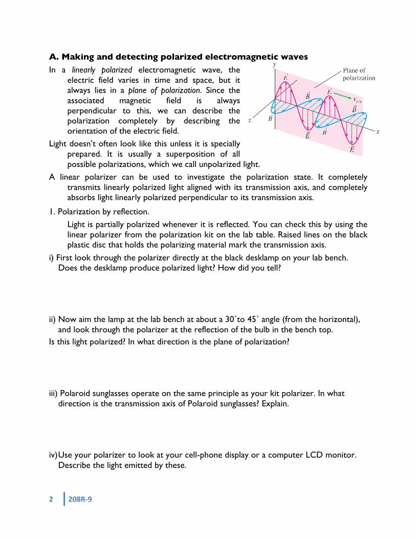
2   208R-­‐9  

A. Making and detecting polarized electromagnetic waves

In a linearly polarized electromagnetic wave, the electric field varies in time and space, but it always lies in a plane of polarization. Since the associated magnetic field is always perpendicular to this, we can describe the polarization completely by describing the orientation of the electric field.

Light doesn’t often look like this unless it is specially prepared. It is usually a superposition of all possible polarizations, which we call unpolarized light.

A linear polarizer can be used to investigate the polarization state. It completely transmits linearly polarized light aligned with its transmission axis, and completely absorbs light linearly polarized perpendicular to its transmission axis.

1. Polarization by reflection. Light is partially polarized whenever it is reflected. You can check this by using the linear polarizer from the polarization kit on the lab table. Raised lines on the black plastic disc that holds the polarizing material mark the transmission axis.

i) First look through the polarizer directly at the black desklamp on your lab bench. Does the desklamp produce polarized light? How did you tell?

ii) Now aim the lamp at the lab bench at about a 30˚to 45˚ angle (from the horizontal), and look through the polarizer at the reflection of the bulb in the bench top.

Is this light polarized? In what direction is the plane of polarization?

iii) Polaroid sunglasses operate on the same principle as your kit polarizer. In what direction is the transmission axis of Polaroid sunglasses? Explain.

iv) Use your polarizer to look at your cell-phone display or a computer LCD monitor.

Describe the light emitted by these.

208R-­‐9   3  

The polariscope

Your polariscope has two polarizers (even though one is called an analyzer!):

The bottom one sits directly over the (unpolarized) incandescent bulb, and is fixed in place. In a two-polarizer system, it is usually called the “polarizer”, since it produces linear polarized light from an unpolarized source.

The top one can rotate. It is usually in-line with the bottom polarizer, but can also be swung to the side. In a light microscope, it is usually called the “analyzer”, since it analyzes whether a sample placed above the bottom polarizer has altered the polarization.

1. Turn on your polariscope and look down into the top polarizer. Describe the

intensity variations while rotating the top polarizer through 360˚.

2. Find the transmission axis of the bottom polarizer with the small polarizer

(mounted in a black plastic ring) from your box. This one has its transmission axis marked with two ridges in the plastic. Explain your procedure and use a piece of masking tape to mark it on the rim of the polariscope.

Find the transmission axis of the top polarizer and mark it also. 3. What angle is between the transmission axes of the two polarizers when there is:

Maximum transmission? What about no transmission?

Unpolaized light

Polarizer

Analyzer

4   208R-­‐9  

B. Transmission through a polarizer: In the previous section, you found that a linear polarizer will transmit a light wave whose electric field vector is parallel to the transmission axis, and blocks (absorbs) one with electric field vector perpendicular to that direction. For angles not 0º or 90º with respect to the transmission axis the polarizer transmits the component of the E-field along the transmission axis and absorbs the rest. B1. Below is the electric field of an electromagnetic wave throughout its period T. It is

linearly-polarized 45˚ away from the y-axis. Draw the x-and y-components.

y

x

y

x

y

x

y

x

y

x

t=0 t=T/6 t=2T/6

y

x

t=3T/6 t=4T/6 t=5T/6

y

x

t=6T/6

If this wave has electric field amplitude Eo and is incident on a polarizer whose transmission axis is aligned along the y-axis, what is the electric field amplitude and polarization direction of the transmitted wave?

208R-­‐9   5  

B1. Set the analyzer on your polariscope so that no light is transmitted. Now insert the small round polarizer from your kit between them and rotate it.

Why does light now get through at some angles? B2. Rotate the middle polarizer through a full 360˚. From your experimental

observations, qualitatively sketch the intensity through the top analyzer vs angle of the middle polarizer transmission axis relative to the transmission axis of the bottom fixed polarizer.

B3. At what angles of the inner polarizer do you get maximum intensity?

Explain.

0˚ 90˚ 180˚ 270˚ 360˚

Kit polarizer

Unpolaized light

6   208R-­‐9  

C. Circular Polarization: The polarization state describes the electric field vector of the EM wave. The most common is the linear polarization of part B. Other polarization states can be understood as the superposition of linear polarization states. Circular polarization is an important one; it is a superposition of waves with a quarter period (90˚) phase shift.

1. The graphs below show the E-fields of the two linearly-polarized waves at time intervals Δt=T/8 (T is the wave period). Draw the vector sum of the two E-fields on each graph below. The vector with the big arrowhead is the E-field of the wave polarized along the y-axis. The vector with the small arrowhead is the E-field of wave polarized along the x-axis, that starts later in time. If a particular vector does not appear, the E-field of that wave at that time is zero.

0 T/8 2T/8 3T/8 4T/8 5T/8

x

y

y

x

y

x

y

x

y

x

y

x

t=0 t=T/8 t=2T/8

y

x

t=3T/8 t=4T/8 t=5T/8

y

x

t=6T/8

y

x

t=7T/8

y

x

t=T

208R-­‐9   7  

Fast axis Slow axis

¼ wave plate

Linear polarizer

Transmission axis

2. Describe the time-dependence of the total E-field (direction and magnitude). Does the magnitude change in time? Does the direction change in time?

When the horizontal component starts ¼ period earlier (-90˚ phase shift) rather than

later, the electric field vector rotates in the opposite direction. These two polarization states are right and left circular.

Making circularly polarized light As you showed above, you can make circularly polarized light by combining two linearly polarized waves, with their plane of polarizations at right angles, and with a relative delay of ¼ wavelength.

There is a very easy way to do this. Some materials are optically anisotropic, meaning that light waves polarized along different directions travel at different speeds. This means that the slower one is delayed relative to the faster one. The thickness of the plate is such that the time delay is ¼ of the wave oscillation period T (equivalent to a ¼ wavelength delay, or 90˚ in phase). These are called ¼-wave plates.

Analyzing circular polarization: Set the ¼ wave plate on the lower polarizer of the polariscope. Align the wave plate so that the linearly polarized light enters with its plane of polarization halfway between the fast and slow axes of the ¼ wave plate. (The fast axis is marked on the brass holder)

Now x- and y-components of the linearly polarized light have equal amplitude, and are aligned with the fast and slow axes of the ¼ wave plate.

4. Explain why this should produce circularly-polarized light.

5. Now rotate the top polarizer. The intensity of the light transmitted through the wave plate remains approximately constant as you rotate the analyzer (top polarizer) [you may need to slightly adjust the wave-plate angle]. Explain why this happens.

8   208R-­‐9  

D. Chiral molecules and polarized light We discuss circular polarization because many molecules interact differently with left-handed and right-handed light due to their molecular “chirality”, or “handedness”. Amino acids (shown at right in both chiralities) and sugars are chiral. Your body uses and produces only D-sugars (right-handed) and only L-amino acids (left-handed). 1. Explain why the molecules in the figure above are not identical. In a biological (right-handed) sugar solution, right and left circularly polarized light interact differently with the right-handed molecules. The result is that the EM waves propagate at different speeds. To observe this, we could have a race between right- and left-circularly polarized light. We would start them at the same time, and see which one arrived first at the other end of the sugar solution. Sounds complicated, but it turns out that right- and left-circularly polarized light together is something you’ve seen before:

2. Below are plots that let you superimpose two EM waves with right and left circular polarizations. At to both have their E-fields pointing along the y-axis. One rotates clockwise and the other counter-clockwise. Add the E-fields as vectors as you did the two linear polarizations in C1. Draw the resultant vector at each time step.

Describe the polarization of the EM wave that is the sum of these two circularly polarized waves. Is it circularly polarized? Linearly polarized? Explain.

to t1 t2

t3 t4 t5

x

y

208R-­‐9   9  

This means that you can race right- and left- circularly polarized light through a chiral solution by sending in linearly polarized light. In D2 above, the right and left-circularly polarized light start together (in-phase), ready to race.

But they propagate at different speeds, so that one will arrive sooner at the other end. This results in a relative delay between right- and left- circular polarization when they leave the chiral solution.

3. Below are plots that let you superimpose the electric field vectors of right and left

circularly polarized EM waves with a relative delay. The left-handed light is delayed

€

φleft −φright( )=90˚ (1/4 period) from the right-handed light. Add the E-fields as vectors

as you did the in D2. Draw the resultant vector at each time step.

Describe the polarization of the sum of these two circularly polarized waves.

4. The relation between the polarization angle θ of the resulting linear polarization, and the relative phase delay

€

φleft −φright between the left- and right-handed polarization

components, is

€

θpol = φleft −φright( ) /2. Explain how this is consistent with the plots you

made in D2 and D3.

to t1 t2

t3 t4 t5

x

y

10   208R-­‐9  

Now you do the experiment, sending linearly polarized light through a concentrated biological sugar solution. We use Karo corn syrup because it is a very concentrated chiral solution of right-handed molecules (sugars) only. If you don’t know what Karo syrup is, call your mother and ask her. She probably hasn’t heard from you in a while, and would enjoy talking with you.

The right- and left-circularly polarized components of the linearly polarized light propagate at different speeds. They start at the same time, but arrive at the other end with a relative delay, which you just showed appears as rotated linearly polarized light.

You have a set of four jars of Karo syrup (three small and one large, with different heights of syrup). Don’t tip them: the syrup takes time to run back down into the jar.

5. Place the large jar (lid off, open end up) on the polarizer and rotate the analyzer while looking through the polarizers and syrup. You should see colors in the syrup. In what order do the colors appear as you rotate the analyzer clockwise?

Since the rotation appears to be different for different colors (wavelengths), place a

color filter (colored transparency) under the syrup so you are only looking at “one color” (see spectral transmission below).

Rotate the analyzer so the light outside the jar is extinguished. Then rotate the analyzer until the light through the syrup is extinguished. The difference of these angles is the angle by which the Karo has rotated the light. 6. What direction (clockwise or counter-clockwise, looking from the top) is the plane

of polarization rotated? How did you tell? (Hint: a little bit of Karo rotates the polarization a little bit, and a lot rotates it more, so look at the jar with a little Karo).

0

20

40

60

80

100

400 500 600 700

Roscolux #122, Green Diffusion

TRA

NS

MIS

SIO

N (

% )

WAVELENGTH ( nm )

0

20

40

60

80

100

400 500 600 700

Roscolux #124, Red Cyc Silk

TRAN

SMIS

SIO

N (

% )

WAVELENGTH ( nm )

208R-­‐9   11  

Record the polarization rotation of the large jar for the red and green filters. Filter color: Relative rotation (deg):

7. Do this for the other jars and record all your data below.

Sugar depth Green angle Red angle

8. Plot the data for the two colors on the axes below.

Sugar Depth (cm)

Pola

rizat

ion

Rot

atio

n (d

eg)

0 2 4 6 8

20

40

60

80

100

0

120

140

12   208R-­‐9  

Now you analyze the data. 9. Suppose that the right-handed component moves at 0.999997 the speed of the left-

handed component (

€

vright /vleft = 0.999997). Then the left-handed component arrives at the top of the syrup a short time

€

Δt before the right-handed component.

What is

€

Δt after traversing 8 cm of Karo? (take

€

vleft =c

nKaro=3×108m /s

1.5= 2 ×108m /s).

The phase difference between the right- and left-handed components depends on the

arrival time difference

€

Δt and on the oscillation period T. For instance

€

Δt = T /2 corresponds to a phase shift of π (180˚).

€

Δt = T /4 gives a phase shift of π/2 (90˚). 10. The peak wavelength of red light you used above is about 660 nm in vacuum.

This has an oscillation period

€

T = λ /c = 2.20 ×10−15 s. What is the phase difference

€

φleft −φright between the left- and right-handed components for the time delay

€

Δt calculated in D9?

11. The peak wavelength of green light you used above is about 520 nm in vacuum.

This has an oscillation period of

€

T = λ /c =1.73×10−15 s What is the phase difference

€

φleft −φright between the left- and right-handed components for the time delay

€

Δt calculated in D9? 12. Using

€

θpol = φleft −φright( ) /2 from D4, what polarization rotations are these?

Red Light rotation: Green Light rotation:

208R-­‐9   13  

13. Why did the same arrival time difference result in different polarization rotations for different colors of light?

14. Explain whether your answer to the question above describes the order of the

colors you observed in D5, assuming that the arrival time delay does not depend on wavelength.

14   208R-­‐9  

This page intentionally blank.

Name_____________________________ Section___________

208-­‐R10   1  

Physics 208 Laboratory Spectroscopy and the hydrogen atom

This sheet is the lab document your TA will use to score your lab. It is to be turned in at the end of lab. To receive full credit you must use complete sentences and explain your reasoning clearly. What’s this lab about? This is the first lab about quantum mechanics. Your goal is to measure emission lines of the Hydrogen atom, and correlate them with transitions of the atom between different quantum states. You do this by measuring the wavelength of photons emitted by Hydrogen atoms in excited quantum states. You use a diffraction grating to disperse the wavelengths at different angles (by constructive interference), and a spectrometer to accurately measure the angles. Why are we doing this? Emission and absorption spectra can be a unique fingerprint of an atom or molecule. The photon energies and wavelengths are directly related to the allowed quantum energy states of the system.

What should I be thinking about before I start this lab? Think about what happens when a quantum system makes a transition from a high-

energy state to a low-energy state. Think about what the quantum states are for a hydrogen atom, and the connection between atomic transitions and photons.

Any safety issues?

The green plastic filter is in front of the Mercury source to block ultraviolet radiation from the bulb, so don’t remove it. The Mercury source also can become very hot – be careful not to touch it, or to let the black cloth rest against it.

Be careful not to touch the metal electrodes attached to the tube of the Hydrogen source. It is relatively high voltage, and can shock you.

2   208-­‐R10  

A. The diffraction grating

The equipment in this lab allows for very accurate measurements of the angles for which constructive interference occurs for light passing through a diffraction grating. Remember from the first lab of the semester that a CD or DVD, consisting of many closely spaced tracks acting as slits, behaves as a reflective diffraction grating. The grating you use in the spectrometer here works in transmission, but is otherwise the same: it has many closely spaced slits, with a density of 600 slits/mm.

This is actually close to the 1.6 µm track spacing that you found for the CD. In that experiment you aimed a red laser at the CD and found that each groove acted as a source of spherical waves, and these canceled by destructive interference except at particular angles

€

θ determined by the wavelength according to

€

mλ = d sinθ . Here d is the slit spacing and m an integer indicating the order of diffraction.

In that experiment you had a single wavelength. Here the incoming light may be made of several different wavelengths. Each wavelength will diffract constructively at particular angles given by the above formula. The job of the spectrometer is to accurately measure those angles, and so determine the wavelengths making up the incoming light.

A1. Suppose you see only four diffracted rays from the diffraction grating, at angles of

€

θ = 20˚ ,

€

θ = 23̊ ,

€

θ = 43.16˚, and

€

θ = 51.4˚. You detect these with your eye, so you know they are all in the visible spectrum. What wavelengths are in the incoming light?

208-­‐R10   3  

B. Measuring the diffracted angle with the spectrometer

The spectrometer has three main pieces (shown below)

1. A collimator (makes rays hitting the diffraction grating parallel)

2. Diffraction grating (discussed above)

3. An observation telescope (to accurately view the spectral lines)

There are also several mechanical adjustments, as shown in the figure above. Don’t

adjust K and L. These are to make the grating perpendicular to the collimator, and to adjust the angle scale so that it indicates 0˚ when the viewing telescope is aligned exactly on the axis of the collimator.

The collimator has a slit on the far end, and a lens on the near end that makes the light rays from the slit parallel. You turn the knurled knob C) to open and close the slit. Opening the slit gives a brighter image, but less angular resolution.

The viewing telescope can be focused, and its angle can be changed. Two adjustments to focus the viewing telescope: i) Slide the eyepiece tube in or out until the crosshairs are in focus. ii) Turn the knurled knob until the image of the slit (lit by desk lamp) is in focus Two ways to move the viewing telescope: i) loosen the telescope clamp and move the telescope with your hand (coarse adjust) ii) tighten the telescope clamp, and turn the fine-adjust knurled knob (fine adjust)

4   208-­‐R10  

C. Using the spectrometer First you look at light from an incandescent bulb. This light appears white to your eye, but is a continuous superposition of all wavelengths in the visible range. You view these wavelengths separately with the spectrometer.

Make sure the grating is in place, and turn on the desk lamp so it shines through the slit. Put the black cloth over the spectrometer to block out stray light. Unlock the telescope and rotate it left and right while viewing to find the continuous spectrum on either side of the central maximum. If you can’t see the continuous spectrum, part of the black cloth may be blocking the light. Try adjusting the slit width.

1. Is the order of the colors what you would expect from sind mθ λ= ? Explain

2. Pick a color or edge of a color in the spectrum with the telescope crosshairs and lock the telescope in place. Use the angle scale and vernier to determine the angle away from the central maximum. (Read carefully the description of measuring angles with the vernier scale on the last page of this handout.)

3. Unlock the telescope and align it with the same color or edge of a color on the

opposite side of the central maximum. Record the angles of the spectrometer away from the central maximum.

4. Average the two angle readings and compute the wavelength of color you chose.

Show your calculations. We use the average to account for slight misalignments of the grating, which should be, but isn’t, exactly perpendicular to the collimator.

208-­‐R10   5  

D. Accurately measure d, the line spacing of the grating

Your grating is a replica grating. It is plastic that is stamped like a CD from a master grating. Because of this it could be slightly stretched or compressed, so that the line spacing is not exactly as written on the grating holder. Here you accurately determine the line spacing by measuring the diffraction angle of the

€

λ = 546.1 nm spectral line of mercury.

Replace the desk lamp with the Hg lamp. Make sure the green safety filter is in place (the filter blocks the UV part of the spectrum).

D1. Following the same procedure as in part C, write down the angles (left and right) for the first order line for λ = 546.1 nm. It is by far the brightest green line in the spectrum. You should be able to see the green line, the doubled yellow line to the left, and some faint blue lines. If you can’t resolve the two yellow lines, reduce the width of the spectrometer entrance slit until you can.

D2. Use the known wavelength and your measured angle for the first order line to calculate d and the lines/mm for your grating. Show all your work and compare the result to the value written on your grating.

Use your measured value for the grating line spacing d in the next section.

6   208-­‐R10  

E. Measuring spectral lines of the hydrogen atom

Replace the Hg lamp with the hydrogen source and position it exactly in front of the slit (if it is not, the lines will not be bright enough to see). Repeat the measurement procedure for every line in the first order spectrum on both sides of the central maximum. Organize your data and calculations in the table at the end of this page.

1. Pick the line (color) farthest from the central maximum and fill in color, angle-left, and angle right in the table.

2. Determine θ from the average and write it in the table also. Show your work here.

3. Using your measured grating line spacing from section D to calculate the wavelength

of the hydrogen spectral line in nm.

4. Calculate the photon energy for this line and show your work here. Use

€

hc =1240 eV ⋅ nm .

5. Before going on make sure your procedure is sound and your numbers make sense. Ask your TA before going on if you are uncertain.

6. Repeat the above process for the rest of the lines in the spectrum to fill in the table. color angle-left angle-right θ λphoton Ephoton

208-­‐R10   7  

F. Atomic energy levels for hydrogen

F1. Using 2

13.6nE eV

n= − , mark the energy levels for

hydrogen on the graph at right.

F2. Determine which transitions are responsible for the spectral lines in your table. Mark those transitions on the energy level diagram with an arrow drawn from the initial state to the final state. Indicate which spectral line (color) goes with which arrow. Explain your reasoning and give examples of why other transitions cannot be responsible for these lines.

E (eV)

0

- 1

- 2

- 3

- 4

- 5

- 6

- 7

- 8

- 9

-10

-11

-12

-13

-14

8   208-­‐R10  

Appendix: Reading the vernier scale on the spectrometer The verniers have 30 divisions per half degree. Hence each division is (1/30)x(1/2) = (1/60)˚ or one minute (') of arc. The knurled ring about the collimator, B, controls the slit opening.

Staff have already focused the collimator for parallel light and have set collimator and telescope perpendicular to spectrometer's rotation axis. REMINDER ON READING A VERNIER

1) Position and tighten the telescope.

2) Move the magnifying glass to see the scale marking

3) Look where the zero mark on the upper scale is located. The degree reading is the first full degree mark to the left of the zero (210˚ in the top figure; 229˚ in the bottom figure).

4) Now make the minute reading: if the zero mark on the upper scale comes after a ½ degree mark (the short lines on the lower scale) then start at 30', otherwise at 0'.

5) Next look for the two lines which match up best between the two scales. Read the number of the appropriate line on the upper scale and add it to the zero mark is just past a degree mark so we begin with 30'. The 15' mark is the one that lines up best so we get 210˚15' for the top reading and 229˚46' for the bottom one.

6) Now convert to decimal degrees, in this case 15/60 = 0.25, so = 210.25˚