physics 143a - quantum mechanics i - github pages · physics 143a notes 5 does not have this...
TRANSCRIPT

Physics 143a - Quantum Mechanics I
Taught by Matthew ReeceNotes by Dongryul Kim
Spring 2017
This course was taught by Matthew Reece, at TTh 10-11:30 in Jefferson356. The textbook was A Modern Approach to Quantum Mechanics by JohnTownsend. There were 34 undergraduates and 1 graduate student enrolled andthe grading was based on weekly problem sets, two in-class midterm, and athree-hour final exam. The teaching fellow was Mobolaji Williams.
Contents
1 January 24, 2017 41.1 Introduction . . . . . . . . . . . . . . . . . . . . . . . . . . . . . . 41.2 Linear superpositions . . . . . . . . . . . . . . . . . . . . . . . . . 4
2 January 26, 2017 62.1 The Stern–Gerlach experiment . . . . . . . . . . . . . . . . . . . 62.2 Unitary transformations . . . . . . . . . . . . . . . . . . . . . . . 7
3 January 31, 2017 83.1 Linear operators . . . . . . . . . . . . . . . . . . . . . . . . . . . 83.2 Rotation matrices . . . . . . . . . . . . . . . . . . . . . . . . . . . 9
4 February 2, 2017 104.1 Projection operators . . . . . . . . . . . . . . . . . . . . . . . . . 11
5 February 7, 2017 125.1 Commutator of rotations . . . . . . . . . . . . . . . . . . . . . . . 125.2 Non-commuting observables and uncertainty . . . . . . . . . . . . 13
6 February 9, 2017 156.1 Representations of su(2) (1) . . . . . . . . . . . . . . . . . . . . . 15
7 February 14, 2017 177.1 Representations of su(2) (2) . . . . . . . . . . . . . . . . . . . . . 177.2 The uncertainty principle . . . . . . . . . . . . . . . . . . . . . . 18
1 Last Update: August 27, 2018

8 February 21, 2017 198.1 Classical story to the Hamiltonian . . . . . . . . . . . . . . . . . 198.2 Time evolution . . . . . . . . . . . . . . . . . . . . . . . . . . . . 19
9 February 23, 2017 229.1 Spin particle in a magnetic field . . . . . . . . . . . . . . . . . . . 22
10 February 28, 2017 2410.1 Position . . . . . . . . . . . . . . . . . . . . . . . . . . . . . . . . 2410.2 Position and momentum operators . . . . . . . . . . . . . . . . . 25
11 March 2, 2017 2711.1 Base change between position and momentum . . . . . . . . . . . 2711.2 Gaussian wave packet . . . . . . . . . . . . . . . . . . . . . . . . 27
12 March 7, 2017 2912.1 Particle in potential . . . . . . . . . . . . . . . . . . . . . . . . . 29
13 March 9, 2017 3113.1 Physical interpretation of oscillating solutions . . . . . . . . . . . 3113.2 Ladder operators . . . . . . . . . . . . . . . . . . . . . . . . . . . 33
14 March 21, 2017 3414.1 The harmonic oscillator . . . . . . . . . . . . . . . . . . . . . . . 34
15 March 23, 2017 3615.1 Coherent states . . . . . . . . . . . . . . . . . . . . . . . . . . . . 36
16 March 30, 2017 3816.1 Particles in three dimension . . . . . . . . . . . . . . . . . . . . . 3816.2 Multiparticle states . . . . . . . . . . . . . . . . . . . . . . . . . . 40
17 April 4, 2017 4117.1 Center-of-mass frame . . . . . . . . . . . . . . . . . . . . . . . . . 41
18 April 6, 2017 4318.1 Orbital angular momentum . . . . . . . . . . . . . . . . . . . . . 4318.2 Particle in a central potential . . . . . . . . . . . . . . . . . . . . 44
19 April 11, 2017 4619.1 Spherical harmonics . . . . . . . . . . . . . . . . . . . . . . . . . 4619.2 Boundary condition for the radial function . . . . . . . . . . . . . 47
20 April 13, 2017 4820.1 Radial function for the Coulomb potential . . . . . . . . . . . . . 49
2
21 April 18, 2017 5121.1 Entangled states . . . . . . . . . . . . . . . . . . . . . . . . . . . 5121.2 Density operator . . . . . . . . . . . . . . . . . . . . . . . . . . . 52
22 April 20, 2017 5322.1 Reduced density operator . . . . . . . . . . . . . . . . . . . . . . 5322.2 Decoherence and interpretation of quantum physics . . . . . . . . 5422.3 Bell’s inequality . . . . . . . . . . . . . . . . . . . . . . . . . . . . 55
23 April 25, 2017 5623.1 A quantum mechanical strategy . . . . . . . . . . . . . . . . . . . 5623.2 No-cloning theorem and quantum transportation . . . . . . . . . 58
3
Physics 143a Notes 4
1 January 24, 2017
There will be weekly problem sets due Tuesdays. There will be two in-classmidterms, on Feb 16 and Mar 28. Our textbook is Townsend, A Modern Ap-proach to Quantum Mechanics, 2nd edition. The main prerequisite will be linearalgebra. You don’t necessarily have to take Physics 15c to take this course.
1.1 Introduction
Quantum mechanics is more of a principle that underlies many theories, e.g.,classical mechanics. There are many forms of classical mechanics. The under-lying principle of Newtonian mechanics is ~F = m~a, the principle in Lagrangianmechanics is ∂L/∂q − (d/dt)∂L/∂q = 0. The universal law in Hamiltonianmechanics is q = ∂H/∂p and p = −∂H/∂q.
Once you have the universal principle, you can study different theories byapplying that law to different situations. Let me list a few of these theories.
• hydrogen atom: its energy levels and transitions (Ch. 10)
• quantum electrodynamics: relativistic theory of EM field (photons), elec-trons, positrons, . . .
• BCS superconductivity: Cooper pairs, . . .
• theory of nuclear matter
• cosmology: inflation and destiny perturbations
• standard model
• string theory
Most of the things here are things we won’t see in the course, but I wanted togive a sense of where you can go with quantum mechanics.
The logic of quantum mechanics is very weird, in the sense that it is differentfrom the classical world. Classical physics emerges from quantum mechanics oflarge numbers of particles. This emergence is largely due to entanglement anddecoherence. We will get a glipse by the end of the semester, but the real worldis quantum mechanical.
1.2 Linear superpositions
Consider the wave equation
∂2
∂t2f(x, t)− ∂2
∂x2f(x, t) = 0.
If f1(x, t) and f2(x, t) are solutions, then c1f1(x, t) + c2f2(x, t) is also a solutionfor any constants c1, c2. However, the equation
∂2
∂t2f(x, t)− ∂2
∂x2f(x, t) = εf(x, t)2

Physics 143a Notes 5
does not have this property.Quantum mechanics postulates that linear superpositions of physical states
are physical states. So linearity is built into quantum mechanics in a fundamen-tal way. This is a postulate that we assume because it matches experiment.
Example 1.1. Let us look at a “qubit”, a quantum bit. The classical bit takesvalues in 0 or 1. What happens in quantum mechanics is that the bit can takeany linear combination:
|ψ〉 = c0|0〉+ c1|1〉
These |0〉 and |1〉 are quantum states corresponding to the classical state, andc0 and c1 are complex numbers. This notation is something like the vectornotation ~v = v1~e1 + v2~e2 in mathematics. Sometimes we might change thenotation, e.g., |↑〉 and |↓〉 if it represents a spin, or |L〉 and |R〉 if it representslight polarization.
When we work with vectors, we take the dot product as
~w · ~v = w1v1 + w2v2 + w3v3 = wT v.
We are going to do something similar with quantum states. Assume we have anorthonormal basis,
〈0|1〉 = 1, 〈1|1〉 = 1, 〈0|1〉 = 0, 〈1|0〉 = 0.
I’ve introduced some funny notation here. For two quantum states |ψ〉 and|χ〉, we write the inner product as 〈χ|ψ〉. Suppose |ψ〉 = c0|0〉 + c1|1〉 and|χ〉 = d0|0〉+ d1|1〉. Then their inner product is
〈χ|ψ〉 = d∗0c0 + d∗1c1.
If we were taking the inner product in the other way, we would get
〈ψ|χ〉 = c∗0d0 + c∗1d1 = (〈χ|ψ〉)∗.
We will choose to work with normal states, i.e., 〈ψ|ψ〉 = 1. Note that if Idefine |ψ′〉 = eiθ|ψ〉 by rephasing it, then 〈ψ′|ψ′〉 = 〈ψ|ψ〉 = 1. Physics doesn’treally care about phase change, and so we can say that quantum states is acomplex vector space modulo scaling and phase change.
The reason we flipped the angle on the right is because the angle on the lefthas a meaning of its own:
if |ψ〉 = c0|0〉+ c1|1〉 then 〈ψ| = c∗0〈0|+ c∗1〈1|.
This is called the Dirac notation. The |ψ〉 is called a ket and 〈ψ| is calleda bra so that the inner product becomes a bracket. We can represent |ψ〉 ascolumn vectors and 〈ψ| as row vectors. In this context, the inner product is likew†v, where † is Hermitian conjugation.
Physics 143a Notes 6
2 January 26, 2017
2.1 The Stern–Gerlach experiment
An electron has an intrinsic spin ~S, and a non-uniform magnetic field exerts aforce. The force is given by
~F ∝ ~S · n.
When (non-polarized) particles pass though a Stern–Gerlach device, it turnsout that there are discrete outcomes observed, not a continuous pattern. Letus write the Stern–Gerlach device that checks the ~S · n by SGn. You can dothe experiment with multiple devices like letting the particles pass tough SGz,choose one of the beams, and then let us pass though SGx. The result is thatthe particles split into two deflection patterns, with 50% chance each.
At the early state of quantum mechanics, there were many confusing exper-iments like this. There is a mathematical formalism that matches the result.Let us write |+n〉 the quantum state that is definitely deflected up and |−n〉the quantum state that is definitely deflected down. Then we can write anyquantum state as
|ψ〉 = c+|+n〉+ c−|−n〉,
where |c+|2 + |c−|2 = 1.Now we make the following assumptions:
• If |ψ〉 goes through an SGn device, and the outgoing particle is detected,we see |+n〉 with probability |c+|2 and |−n〉 with probability |c−|2.
• After measuring, the state is is |+n〉 or |−n〉.
It turns out that the state space for an electron’s spin is really 2-dimensional.So we can choose a basis and write |ψ〉 = c+|+z〉 + c−|−z|. There should bestates |+x〉 and |−x〉 and so there must be presentations
|+x〉 = c+|+z〉+ c−|−z〉, |−x〉 = d+|+z〉+ d−|−z〉,
with |c+|2 = |c−|2 = |d+|2 = |d−|2 = 1/2 and d∗+c+ + d∗−c− = 0. There will alsobe states in the y direction. If you solve the equation, you can choose the states
|+x〉 =1√2|+z〉+
1√2|−z〉, |−x〉 =
1√2|+z〉 − 1√
2|−z〉
work. If you solve the equations, you see that
|+y〉 =1√2|+z〉+
i√2|−z〉, |−y〉 =
1√2|+z〉 − i√
2|−z〉
work.
Physics 143a Notes 7
2.2 Unitary transformations
For a vector |ψ〉+ c+|+z〉+ c−|−z〉, we associate a vector (c+ c−)T . If we havethe same vector in another bases, say |ψ〉 = c′+|+x〉+ c′−|−x〉, then(
c′+c′−
)=
(1/√
2 1/√
2
1/√
2 −1/√
2
)(c+c−
).
If we note |+z〉 = (〈+x|+ z〉)|+x〉+ (〈−x|+ z〉)|−x〉, we can abstractly write(〈+x|ψ〉〈−x|ψ〉
)=
(〈+x|+ z〉 〈+x| − z〉〈−x|+ z〉 〈−x| − z〉
)(〈+z|ψ〉〈−z|ψ〉
).
This matrix is unitary, i.e., U†U = UU† = 1. This is because
U =
(〈+x|+ z〉 〈+x| − z〉〈−x|+ z〉 〈−x| − z〉
), U† =
(〈+z|+ x〉 〈+z| − x〉〈−z|+ x〉 〈−z| − x〉
).
Note that the U† is then going from the x-basis to the z-basis. This shows thatU†U = 1.

Physics 143a Notes 8
3 January 31, 2017
One remark I would like to make is that when we measure the spin ~S, itsmagnitude is
|S| = ~2, ~ ≈ 6.6× 10⁻¹⁶eV · sec ≈ 1.1× 10⁻³⁴J · s.
Because this is a fundamental constant in nature, this allows us to write timeas inverse energy, or distance as inverse momentum. The reason why particlephysicists like to see what happens when particles collide with large momentumis because they want to know things in small length scale.
One other thing is, if you have a device that is a like SGz plus SG(−z) sothat the result is always the same, then you get |ψ〉 again. This is because wedon’t measure the state of the particle. A measurement is any physical processthat “strongly” depends on the result. When you measure something in a lab,you usually have something like when an electron comes in then some materialabsorb it and emits lots of photons. This kind of transports the information fromthe electron to the material. In short, the laws of quantum mechanics applies toeverything including measuring devices and there is nothing too special aboutmeasuring. It is just that the device has a complex structure and it is hard tofollow all the details in the device.
Finally, in the homework you found out that
|+n〉 = cosθ
2|+z〉+ eiφ sin
θ
2|−z〉.
Now this has two parameters θ and φ and so it is a 2-dimensional state. Ageneral quantum state is of the form α|+z〉+ β|−z〉 and so there are 4 degreesof freedom. In quantum mechanics we normalize our states and so that leaves 3.But we also don’t care about phase so that leaves 2. So there are 2 importantreal degrees of freedom, parameterized by
CP1 = {(z1, z2) ∈ C2 : (z1, z2) ∼ λ(z1, z2)}.
So problem 1.3 can be thought as giving a link S2 ∼= CP1.
3.1 Linear operators
Given a matrix M , its entries can be read of as Mij = eTi MeTj . So in quantummechanics, given basis states |1〉, |2〉, . . . , |n〉, we have
〈m|n〉 = δmn =
{1 m = n
0 m 6= n,Mij = 〈i|M |j〉.
We normalize states |ψ〉 to compute probabilities. But in general we do notnormalize M |ψ〉.
Physics 143a Notes 9
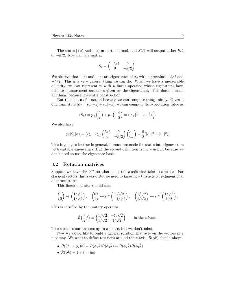
The states |+z〉 and |−z〉 are orthonormal, and SGz will output either ~/2or −~/2. Now define a matrix
Sz =
(+~/2 0
0 −~/2
).
We observe that |+z〉 and |−z〉 are eigenstates of Sz with eigenvalues +~/2 and−~/2. This is a very general thing we can do. When we have a measurablequantity, we can represent it with a linear operator whose eigenstates havedefinite measurement outcomes given by the eigenvalues. This doesn’t meananything, because it’s just a construction.
But this is a useful notion because we can compute things nicely. Given aquantum state |ψ〉 = c+|+z〉+ c−|−z〉, we can compute its expectation value as
〈Sz〉 = p+
(~2
)+ p−
(−~
2
)= (|c+|2 − |c−|2)
~2.
We also have
〈ψ|Sz|ψ〉 =(c∗+ c∗−
)(~/2 00 −~/2
)(c+c−
)=
~2
(|c+|2 − |c−|2).
This is going to be true in general, because we made the states into eigenvectorswith suitable eigenvalues. But the second definition is more useful, because wedon’t need to use the eigenstate basis.
3.2 Rotation matrices
Suppose we have the 90◦ rotation along the y-axis that takes +z to +x. Forclassical vectors this is easy. But we need to know how this acts on 2-dimensionalquantum states.
This linear operator should map(10
)7→(
1/√
2
1/√
2
),
(01
)7→ eiϕ
(1/√
2
−1/√
2
),
(1/√
2
i/√
2
)7→ eiϕ
′(
1/√
2
i√
2
).
This is satisfied by the unitary operator
R(π
2j)
=
(1/√
2 −1/√
2
1/√
2 1/√
2
)in the z-basis.
This matches our answers up to a phase, but we don’t mind.Now we would like to build a general rotation that acts on the vectors in a
nice way. We want to define rotations around the z-axis. R(φk) should obey:
• R((φ1 + φ2)k) = R(φ1k)R(φ2k) = R(φ2k)R(φ1k)
• R(φk) = 1 + (· · · )dφ.

Physics 143a Notes 10
4 February 2, 2017
We want a family of rotations given by R(θ, n). It is reasonable to ask thatif we do a rotation by θ1 then do a rotation by θ2 the result is a rotation byθ1 +θ2. Another thing we would like to require is that rotation by a small angleis almost the identity. This can be written as R(dφk) = 1 + Mdφ+O(dφ2). Weare going to write M = −i/~Jz for reasons that will become clear later.
We can write
R(Ndφk) = R(dφk)N =(
1− i
~Jzdφ+O(dφ2)
)N,
where φ = Ndφ. Thus
R(φk) = limN→∞
(1− i
~Jzφ
N
)N= exp
(− i~Jzφ
),
where exp(M) = 1 + M + M2/2 + M3/6 + · · · . This may seem intimidatingto compute, but there is a nice trick. If M is a diagonal matrix with diagonalentries m1, . . . ,mn, then
exp(M) = 1 +
m1 0. . .
0 mn
+1
2
m21 0
. . .
0 m2n
+ · · · =
em1 0
. . .
0 emn
.
For general matrices, we can diagonalize it and apply this formula. If M =UDU−1 then
exp(M) = exp(UDU−1) =
∞∑n=0
1
n!UDnU−1 = U exp(D)U−1.
Because the rotation matrices must not change the probability and innerproducts, we need R(φk) to be unitary. If we take φ to be a very small angle,we have
R ≈ 1− i
~Jzdφ, R−1 ≈ 1 +
i
~Jzdφ, R+ ≈ 1 +
i
~J+z dφ.
So unitarity of R implies Jz = J+z . That is, Jz is hermitian.
We also want R(φk)|+z〉 to be equal to |+z〉 possibly up to some phase
change. So we we want R(φk) and Jz to be diagonal matrices. We would also
want R(π/2k) to send |+x〉 to |+y〉 up to some phase. If you work these outand make some choices, you can see that
Jz =
(~/2 00 −~/2
)works.
Physics 143a Notes 11
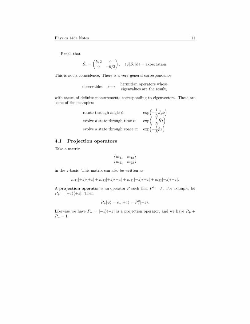
Recall that
Sz =
(~/2 00 −~/2
), 〈ψ|Sz|ψ〉 = expectation.
This is not a coincidence. There is a very general correspondence
observables ←→ hermitian operators whoseeigenvalues are the result,
with states of definite measurements corresponding to eigenvectors. These aresome of the examples:
rotate through angle φ: exp(− i~Jzφ
)evolve a state through time t: exp
(− i~Ht)
evolve a state through space x: exp(− i~px)
4.1 Projection operators
Take a matrix (m11 m12
m21 m22
)in the z-basis. This matrix can also be written as
m11|+z〉〈+z|+m12|+z〉〈−z|+m21|−z〉〈+z|+m22|−z〉〈−z|.
A projection operator is an operator P such that P 2 = P . For example, letP+ = |+z〉〈+z|. Then
P+|ψ〉 = c+|+z〉 = P 2+|+z〉.
Likewise we have P− = |−z〉〈−z| is a projection operator, and we have P+ +P− = 1.
Physics 143a Notes 12
5 February 7, 2017
This is going to be a midterm on Thursday, February 16. You will be given aformula sheet, which will be posted online soon. The reason we are having anexam early is that I want some feedback before the add-drop deadline.
We had these operators Jx, Jy, Jz, which are hermitian and have eigenvaluesand eigenvectors corresponding to measurement outcomes and states. We alsohad these rotations R(φk) = exp(−i/~Jzφ), which are unitary. These rotationsare generated by J .
5.1 Commutator of rotations
The rotations don’t commute in general; rotation by 90◦ around the x-axis andaround the z-axis do not commute. So although we have
R((φ1 + φ2)k) = R(φ1k)R(φ2k),
we don’t have R(φk)R(θj) 6= R(θj)R(φk). One way to measure the failure ofthis is to introduce the commutator
[A, B] = AB − BA.
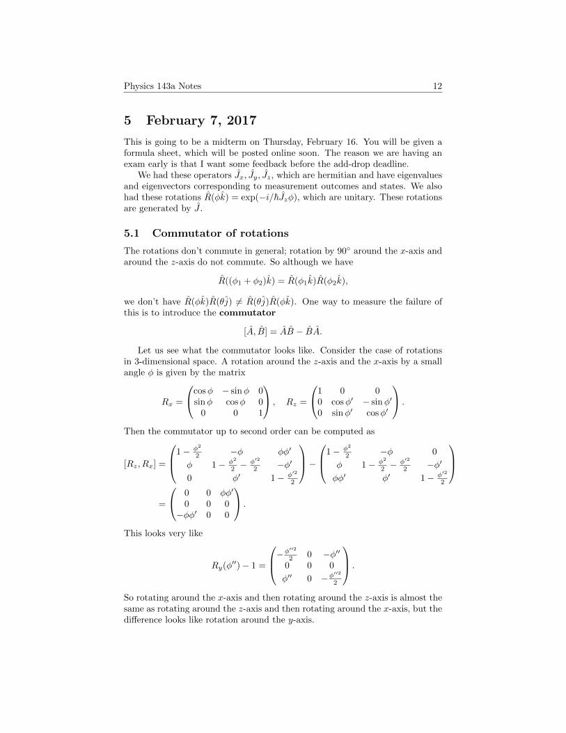
Let us see what the commutator looks like. Consider the case of rotationsin 3-dimensional space. A rotation around the z-axis and the x-axis by a smallangle φ is given by the matrix
Rx =
cosφ − sinφ 0sinφ cosφ 0
0 0 1
, Rz =
1 0 00 cosφ′ − sinφ′
0 sinφ′ cosφ′
.
Then the commutator up to second order can be computed as
[Rz, Rx] =
1− φ2
2 −φ φφ′
φ 1− φ2
2 −φ′2
2 −φ′
0 φ′ 1− φ′2
2
−1− φ2
2 −φ 0
φ 1− φ2
2 −φ′2
2 −φ′
φφ′ φ′ 1− φ′2
2
=
0 0 φφ′
0 0 0−φφ′ 0 0
.
This looks very like
Ry(φ′′)− 1 =
−φ′′2
2 0 −φ′′0 0 0
φ′′ 0 −φ′′2
2
.
So rotating around the x-axis and then rotating around the z-axis is almost thesame as rotating around the z-axis and then rotating around the x-axis, but thedifference looks like rotation around the y-axis.
Physics 143a Notes 13
We can also see this by looking at the generating matrices. We have R(φk) ≈1− i/~Jzφ. So
[Rz(φ), Rx(φ′)] ≈ [−i/~Jzφ,−i/~Jxφ′] = (−i/~)2φφ′[Jz, Jx]
≈ −i/~Jy(φφ′).
So we get
[Jz, Jx] = i~Jy,
and similarly
[Jx, Jy] = i~Jz, [Jy, Jz] = i~Jx.
5.2 Non-commuting observables and uncertainty
Let us first look at commuting observables. It is a fact that
~J2 = J2x + J2
y + J2z
commutes with Jx, Jy, Jz. Suppose we have a Stern-Gerlach device that can
measure Jz, and suppose we have another device that measures ~J2.Suppose we measure a particle using a SGz device. Take the particles that
give |+z〉, measure its J2, and then again measure using SGz. In this case thefirst outcome is always 3/4~2 and the second outcome is always |+z〉.
On the other hand, if you replace J2 with a SGx device, we know that theresults will split in the first outcome, and even if we use only the |+x〉 we againget a split result.
The first experiment is related to the fact that [ ~J2, Jz] = 0 but [Jx, Jz] 6= 0.That is, commuting observables can be measured without changing each other’svalues, while non-commuting observables cannot be measured without affectingeach other.
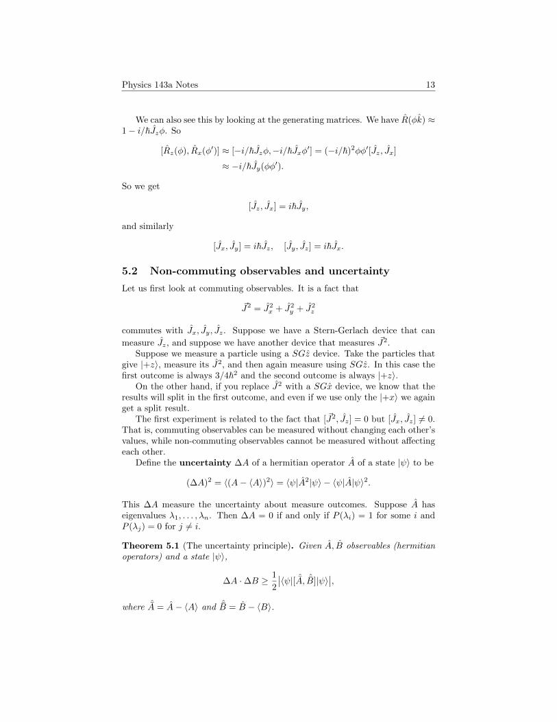
Define the uncertainty ∆A of a hermitian operator A of a state |ψ〉 to be
(∆A)2 = 〈(A− 〈A〉)2〉 = 〈ψ|A2|ψ〉 − 〈ψ|A|ψ〉2.
This ∆A measure the uncertainty about measure outcomes. Suppose A haseigenvalues λ1, . . . , λn. Then ∆A = 0 if and only if P (λi) = 1 for some i andP (λj) = 0 for j 6= i.
Theorem 5.1 (The uncertainty principle). Given A, B observables (hermitianoperators) and a state |ψ〉,
∆A ·∆B ≥ 1
2
∣∣〈ψ|[ ˆA, ˆB]|ψ〉∣∣,
where ˆA = A− 〈A〉 and ˆB = B − 〈B〉.

Physics 143a Notes 14
Proof. Define two kets (not necessarily normalized)
|x〉 = ˆA|ψ〉 = (A− 〈A〉)|ψ〉,
|y〉 = i ˆB|ψ〉 = i(B − 〈B〉)|ψ〉.
These states are constructed so that
〈x|x〉 = 〈ψ|(A− 〈A〉)2|ψ〉 = (∆A)2.
Similarly 〈y|y〉 = (∆B)2. By the Cauchy–Schwartz inequality,
〈x|x〉〈y|y〉 ≥ 1
4
∣∣〈x|y〉+ 〈y|x〉∣∣2.
Now
〈x|y〉 = i〈ψ| ˆA ˆB|ψ〉, 〈y|x〉 = −i〈ψ| ˆB ˆA|ψ〉.
So we get the inequality.

Physics 143a Notes 15
6 February 9, 2017
6.1 Representations of su(2) (1)
Last time we say that [Jx, Jy] = i~Jz ad that ~J2 = J2x + J2
y + J2z commute with
Jx, Jy, and Jz.These are what mathematicians call Lie algberas. They are collections of
objects with addition and the commutator [x, y] satisfying the Jacobi identity
[[x, y], z] + [[y, z], x] + [[z, x], y] = 0.
The physical interpretation is that these things correspond to some symmetries.In this class we are not going to see the general theory. This specific algebra ofJx, Jy, Jz is su(2). We can write rotations as 3 × 3 matrices and also as 2 × 2complex matrices. These two are different representations of su(2).
For ~J2 = J2x + J2
y + Jz, we claim that [ ~J2, Jx] = 0. This is because
[ ~J2, Jx] = [J2x , Jx] + [J2
y , Jx] + [J2z , Jx]
= 0 + Jy[Jy, Jx] + [Jy, Jx]J + Jz[Jz, Jx] + [Jz, Jx]Jz
= −i~JyJz − i~JzJy + i~JzJy + i~JyJz = 0.
Similarly [ ~J2, Jy] = [ ~J2, Jz] = 0. Also ~J2 is hermitian. Note that all the statesof a spin-1/2 particle is an eigenvector with eigenvalue 3/4~2.
Here are some examples satisfying the commutation relations. First we takethe matrices
Jx =~2
(0 11 0
), Jy =
~2
(0 −ii 0
), Jz =
~2
(1 00 −1
),
or alternatively, Ji = ~/2σi where σi are the Pauli matrices. Then ~J2 = 3~2
4 .We can also take
Jx =~√2
0 1 01 0 10 1 0
, Jy =~√2
0 −i 0i 0 −i0 i 0
, Jz = ~
1 0 00 0 00 0 −1
.
These also satisfies the relations [Jx, Jy] = i~Jz mathematically, but it has~J2 = 2~2. So different choices of matrices may give different ~J2.
There is a systematic way to find all such representations. Because [ ~J2, Jz] =0, they share the same eigenstates. Suppose I have a state |λ,m〉 such that
~J2|λ,m〉 = ~2λ|λ,m〉, Jz|λ,m〉 = ~m|λ,m〉.
We have 〈λ,m| ~J2|λ,m〉 = λ~2 because our states are normalized. On the otherhand,
〈λ,m| ~J2|λ,m〉 = 〈λ,m|J2x |λ,m〉+ 〈λ,m|J2
y |λ,m〉+ ~2m2 ≥ ~2m2.
Physics 143a Notes 16
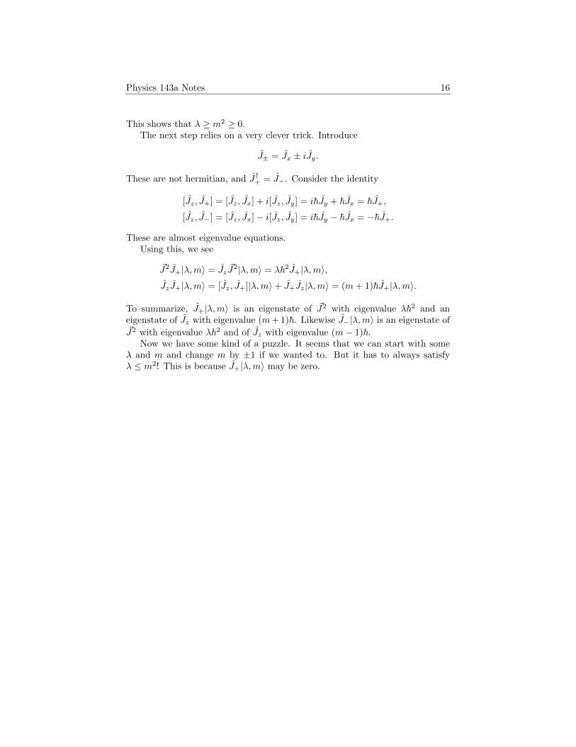
This shows that λ ≥ m2 ≥ 0.The next step relies on a very clever trick. Introduce
J± = Jx ± iJy.
These are not hermitian, and J†+ = J−. Consider the identity
[Jz, J+] = [Jz, Jx] + i[Jz, Jy] = i~Jy + ~Jx = ~J+,
[Jz, J−] = [Jz, Jx]− i[Jz, Jy] = i~Jy − ~Jx = −~J+.
These are almost eigenvalue equations.Using this, we see
~J2J+|λ,m〉 = Jz ~J2|λ,m〉 = λ~2J+|λ,m〉,
JzJ+|λ,m〉 = [Jz, J+]|λ,m〉+ J+Jz|λ,m〉 = (m+ 1)~J+|λ,m〉.
To summarize, J+|λ,m〉 is an eigenstate of ~J2 with eigenvalue λ~2 and aneigenstate of Jz with eigenvalue (m+ 1)~. Likewise J−|λ,m〉 is an eigenstate of~J2 with eigenvalue λ~2 and of Jz with eigenvalue (m− 1)~.
Now we have some kind of a puzzle. It seems that we can start with someλ and m and change m by ±1 if we wanted to. But it has to always satisfyλ ≤ m2! This is because J+|λ,m〉 may be zero.

Physics 143a Notes 17
7 February 14, 2017
We had the commutation relation [Jx, Jy] = i~Jz and [ ~J2, Jx] = 0. We define
J± = Jx ± iJy and showed that
[Jz, J±] = ±~J±,
which resembles the eigenvalue equation. For a eigenstate |λ,m〉 with
~J2|λ,m〉 = λ~2|λ,m〉, Jz|λ,m〉 = m~|λ,m〉,
we showed that λ ≥ m2 and that J± is proportional to |λ,m ± 1〉. This is thereason we introduced J±: the relation [Jz, J±] = ±~J± means that J± add orsubtract ~ from the Jz-eigenvalue.
So this means that we can act by J+ or J− to increase or decrease m by 1.This means that given |λ,m〉, the procedure has to stop somewhere.
7.1 Representations of su(2) (2)
For a fixed λ, label the largest m that makes sense as j. In other words, thereis a state |λ, j| with J+|λ, j〉 = 0. Additional we cam assume that no |λ, j + 1|exists. We know that J−J+|λ, j〉 = 0. Let us expand this out. We get
0 = (Jx − iJy)(Jx + iJy)|λ, j〉 = (J2x + J2
y + i[Jx, Jy])|λ, j〉
= ( ~J2 − J2z − ~Jz)|λ, j〉 = ~2(λ− j2 − j)|λ, j〉.
This implies that λ = j(j + 1). We check that for a spin-1/2 particle, λ =(1/2)(3/2) = 3/4. This agrees with what we know.
We now learned the relationship between λ (the eigenvalue of ~J2) and thelargest eigenvalue of Jz in the ladder, which is given by λ = j(j + 1). We cando this in the other direction. Consider the most negative eigenvalue j so thatJ−|λ, j〉 = 0. Then we would get λ = j(j − 1).
Because
λ = j(j + 1) = j(j − 1),
we have either j = −j or j = j + 1. But the latter doesn’t make sense becausej is the minimum. So we get j = −j.
Now we derived that J−|λ,m〉 = 0 only if m = −j. So if we want Jk−|λ, j〉 = 0for some large enough k, then we need −j to be j minus an integer. Thus j isan half-integer.
Now because j is nicer than λ, we introduce this new notation
~J2|j,m〉 = j(j + 1)~2|j,m〉, Jz|j,m〉 = m~|j,m〉.
A spin-j representation of angular momentum algebra has a basis |j,m〉for m = −j,−j + 1, . . . , j − 1, j. So a spin-0 representation has basis |0, 0〉, aspin-1/2 representation has basis |1/2, 1/2〉 = |+z〉 and |1/2,−1/2〉 = |−z〉.
Physics 143a Notes 18
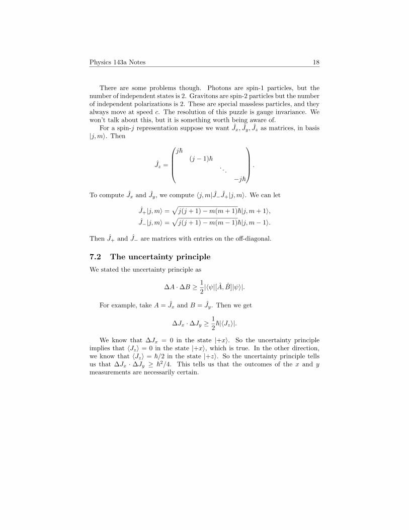
There are some problems though. Photons are spin-1 particles, but thenumber of independent states is 2. Gravitons are spin-2 particles but the numberof independent polarizations is 2. These are special massless particles, and theyalways move at speed c. The resolution of this puzzle is gauge invariance. Wewon’t talk about this, but it is something worth being aware of.
For a spin-j representation suppose we want Jx, Jy, Jz as matrices, in basis|j,m〉. Then
Jz =
j~
(j − 1)~. . .
−j~
.
To compute Jx and Jy, we compute 〈j,m|J−J+|j,m〉. We can let
J+|j,m〉 =√j(j + 1)−m(m+ 1)~|j,m+ 1〉,
J−|j,m〉 =√j(j + 1)−m(m− 1)~|j,m− 1〉.
Then J+ and J− are matrices with entries on the off-diagonal.
7.2 The uncertainty principle
We stated the uncertainty principle as
∆A ·∆B ≥ 1
2|〈ψ|[A, B]|ψ〉|.
For example, take A = Jx and B = Jy. Then we get
∆Jx ·∆Jy ≥1
2~|〈Jz〉|.
We know that ∆Jx = 0 in the state |+x〉. So the uncertainty principleimplies that 〈Jz〉 = 0 in the state |+x〉, which is true. In the other direction,we know that 〈Jz〉 = ~/2 in the state |+z〉. So the uncertainty principle tellsus that ∆Jx · ∆Jy ≥ ~2/4. This tells us that the outcomes of the x and ymeasurements are necessarily certain.

Physics 143a Notes 19
8 February 21, 2017
If you want to compute the exponential of a matrix, you should first diagonalizeit.
In Chapter 4, we are going to learn time evolution and the Hamiltonian. InChapter 6, we are going to deal with continuous systems, position, momentum.Then we would need to solve differential equation. In Chapter 7, we are goingto look at the example of a quantum harmonic oscillator.
8.1 Classical story to the Hamiltonian
In classical mechanics we study the “phase space” given by positions xi andmomenta pi. The key function is the Hamiltonian H, which is a function of thexis and pis. We interpret this as the total energy of the system.
Example 8.1. For a non-relativistic particle with mass m in a potential V , wehave
H =p2
2m+ V (x).
The equations of motion in Hamiltonian mechanics is given by
xi =∂H
∂pi, pi = −∂H
∂xi.
So in the case of a non-relativistic particle, we recover
∂H
∂p=
p
m= x, p = −∂H
∂x= −∂V
∂x= F.
This is precisely Newton’s laws.Given a function f(xi, pi, t), we have
df
dt=∂f
∂t+∑i
[ ∂f∂xi
dxidt
+∂f
∂pi
dpidt
]=∂f
∂t+∑i
[ ∂f∂xi
∂H
∂pi− ∂f
∂pi
∂H
∂xi
]=∂f
∂t+ {f,H},
where {f, g} is the Poisson bracket. This Poisson bracket is some complicatedobject that is not intuitive at all, in classical mechanics. In quantum mechanics,these become simply commutators of Hermitian operators.
8.2 Time evolution
The problem we want to solve is, given a quantum state |ψ(0)〉, what is |ψ(t)〉?We expect it to look like |ψ(t)〉 = U(t)|ψ(0)〉. We like to keep our state nor-malized, so we want U(t) to be unitary. We also expect that if dt is small, thenU(dt) = 1 +O(dt). It is reasonable to also assume
U(t1 + t2) = U(t1)U(t2) = U(t2)U(t1).
Physics 143a Notes 20
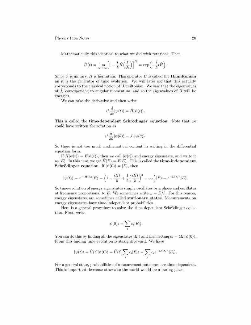
Mathematically this identical to what we did with rotations. Then
U(t) = limN→∞
[1− i
~H( tN
)]N= exp
(− i~tH).
Since U is unitary, H is hermitian. This operator H is called the Hamiltonianan it is the generator of time evolution. We will later see that this actuallycorresponds to the classical notion of Hamiltonian. We saw that the eigenvaluesof Jz corresponded to angular momentum, and so the eigenvalues of H will beenergies.
We can take the derivative and then write
i~d
dt|ψ(t)〉 = H|ψ(t)〉.
This is called the time-dependent Schrodinger equation. Note that wecould have written the rotation as
i~d
dθ|ψ(θ)〉 = Jz|ψ(θ)〉.
So there is not too much mathematical content in writing in the differentialequation form.
If H|ψ(t)〉 = E|ψ(t)〉, then we call |ψ(t)〉 and energy eigenstate, and write itas |E〉. In this case, we get H|E〉 = E|E〉. This is called the time-independentSchrodinger equation. If |ψ(0)〉 = |E〉, then
|ψ(t)〉 = e−iHt/~|E〉 =(
1− iHt
~+
1
2
( iHt~
)2
− · · ·)|E〉 = e−iEt/~|E〉.
So time-evolution of energy eigenstates simply oscillates by a phase and oscillatesat frequency proportional to E. We sometimes write ω = E/~. For this reason,energy eigenstates are sometimes called stationary states. Measurements onenergy eigenstates have time-independent probabilities.
Here is a general procedure to solve the time-dependent Schrodinger equa-tion. First, write
|ψ(0)〉 =∑i
ci|Ei〉.
You can do this by finding all the eigenstates |Ei〉 and then letting ci = 〈Ei|ψ(0)〉.From this finding time evolution is straightforward. We have
|ψ(t)〉 = U(t)|ψ(0)〉 = U(t)∑i
ci|Ei〉 =∑i
cie−iEit/~|Ei〉.
For a general state, probabilities of measurement outcomes are time-dependent.This is important, because otherwise the world would be a boring place.

Physics 143a Notes 21
Given a hermitian operator A, we have
d
dt〈A〉(t) =
d
dt〈ψ(t)|A(t)|ψ(t)〉
=( ddt〈ψ(t)|
)A(t)|ψ(t)〉+ 〈ψ(t)|
( ∂∂tA(t)
)|ψ(t)〉+ 〈ψ(t)|A(t)
( ddt|ψ(t)〉
)= 〈ψ(t)| ∂
∂tA|ψ(t)〉+
i
~〈ψ(t)|[H, A(t)]|ψ(t)〉.
So
d〈A〉dt
=⟨∂A∂t
⟩+i
~〈[H,A]〉.
This is the quantum analogue of the formula df/dt = ∂f/∂t− {H, f}.
Physics 143a Notes 22
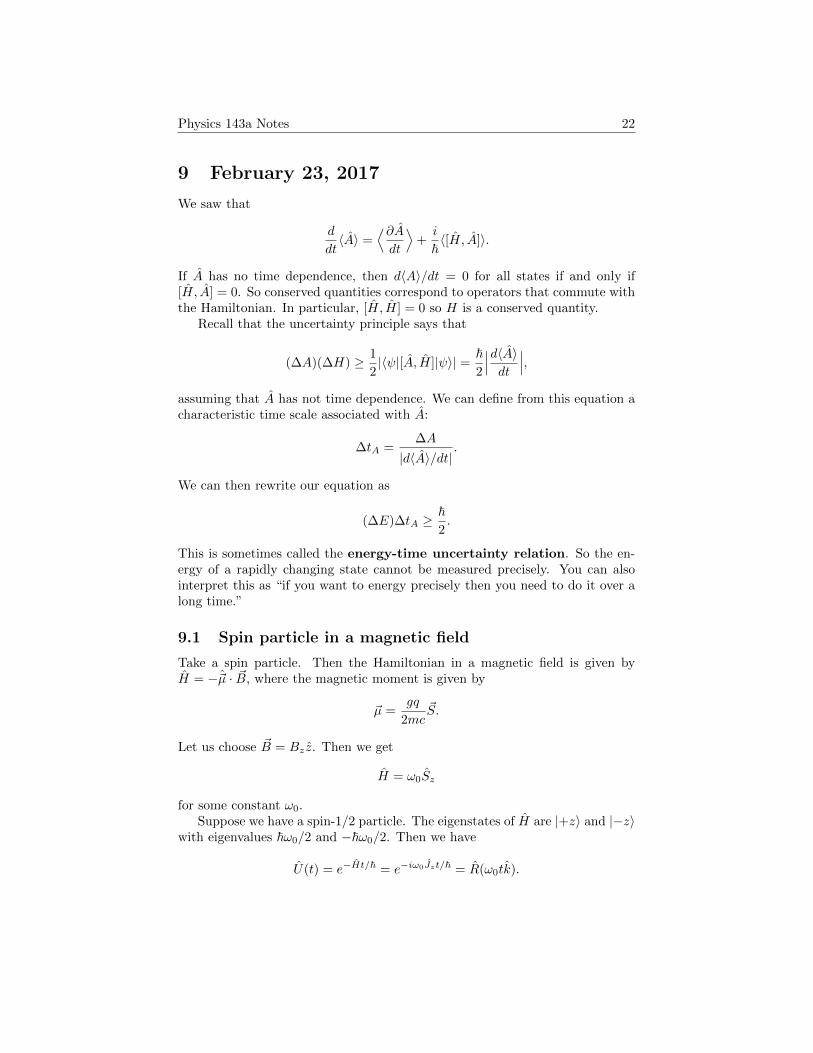
9 February 23, 2017
We saw that
d
dt〈A〉 =
⟨∂Adt
⟩+i
~〈[H, A]〉.
If A has no time dependence, then d〈A〉/dt = 0 for all states if and only if[H, A] = 0. So conserved quantities correspond to operators that commute withthe Hamiltonian. In particular, [H, H] = 0 so H is a conserved quantity.
Recall that the uncertainty principle says that
(∆A)(∆H) ≥ 1
2|〈ψ|[A, H]|ψ〉| = ~
2
∣∣∣d〈A〉dt
∣∣∣,assuming that A has not time dependence. We can define from this equation acharacteristic time scale associated with A:
∆tA =∆A
|d〈A〉/dt|.
We can then rewrite our equation as
(∆E)∆tA ≥~2.
This is sometimes called the energy-time uncertainty relation. So the en-ergy of a rapidly changing state cannot be measured precisely. You can alsointerpret this as “if you want to energy precisely then you need to do it over along time.”
9.1 Spin particle in a magnetic field
Take a spin particle. Then the Hamiltonian in a magnetic field is given byH = −~µ · ~B, where the magnetic moment is given by
~µ =gq
2mc~S.
Let us choose ~B = Bz z. Then we get
H = ω0Sz
for some constant ω0.Suppose we have a spin-1/2 particle. The eigenstates of H are |+z〉 and |−z〉
with eigenvalues ~ω0/2 and −~ω0/2. Then we have
U(t) = e−Ht/~ = e−iω0Jzt/~ = R(ω0tk).

Physics 143a Notes 23
So, for instance, if |ψ(0)〉 = |+x〉 we get
|ψ(t)〉 = U(t)|ψ(0)〉 = |+ cos(ω0t)x+ sin(ω0t)y〉
up to a phase.Now let us take a magnetic field
~B = B0k +B1 cos(ωt)i.
Then our Hamiltonian is H = ω0Sz + ω1 cos(ωt)Sx. The equation we have tosolve is
~2
(ω0 ω1 cosωt
ω1 cosωt −ω0
)(a(t)b(t)
)= i~
(da/dtdb/dt
).
We solve in the special case when ω1 � ω0. The strategy we are going toexploit is to write (
a(t)b(t)
)=
(c(t)e−iω0t/2
d(t)eiω0t/2
).
If ω1 = 0 then c(t) and d(t) are constants. If you just plug in the equation, weget
i
(dc/dtdd/dd
)=ω1
2cosωt
(d(t)eiω0t
c(t)e−iω0t
)=ω1
4
((ei(ω0−ω)t + ei(ω0+ω)t)d(t)
(e−i(ω0−ω)t + e−i(ω0+ω)t)c(t)
).
If ω0 = ω, then ei(ω0+ω)t average to zero. So then we get the smeared equation
i
(dc/dtdd/dt
)=ω1
4
(dc
).
This gives the approximate solution that are linear combinations of e±iω1t/4.

Physics 143a Notes 24
10 February 28, 2017
We are now going to look at continuous space. This is Chapter 6 of Townsend.
10.1 Position
Suppose there is a particle with discrete position so that particles can only beat positions x1, . . . , xn. Then the quantum state can be written as
|ψ〉 =
n∑i=1
ci|xi〉.
This is very much like what we have been doing so far. We would have 〈xi|xj〉 =δij . For instance, you might have some laboratory experiment where there arefinitely many potential wells. But more commonly we are used to continuousspace.
We generalize this to a continuous quantity. We have position x, which isa continuous quantity. Our state is going to be parametrized by a continuousfunction ψ(x), often called the wave function of the state.
In this case, the probability of the particle being at exactly position 0 isgoing to be zero. But we have this probability density
ψ(x) = 〈x|ψ〉.
Then the probability of the particle being found at x0 ≤ x ≤ x1 is∫ x1
x0
dx|ψ(x)|2 =
∫ x1
x0
dx|〈x|ψ〉|2.
We also note that we can also write
|ψ〉 =
∫ ∞−∞
(〈x|ψ〉)|x〉 =
∫ ∞−∞
dxψ(x)|x〉.
We note that we are only looking at position now, and we are going to ignorespin. You can look at particles that have both spin and position, but we aregoing to ignore these to make things simpler.
Analogously to the discrete case, we are going to define the inner product as
〈χ, ψ〉 =
∫dxχ∗(x)ψ(x).
A normalized state satisfies
〈ψ|ψ〉 =
∫dxψ∗(x)ψ(x) =
∫dx|ψ(x)|2 = 1.
We want |ψ〉 to have no units, because they are normalized. This implies
that ψ(x) has units of length−1/2 and so |x〉 also has units of length−1/2. The
Physics 143a Notes 25
position eigenstate |x〉 is not really a state, and in particular, 〈x|x〉 6= 1. Ourposition eigenstates of the inner product
〈x|x′〉 = δ(x− x′),
where δ is the Dirac delta. This is the closest we can get to orthonormality.
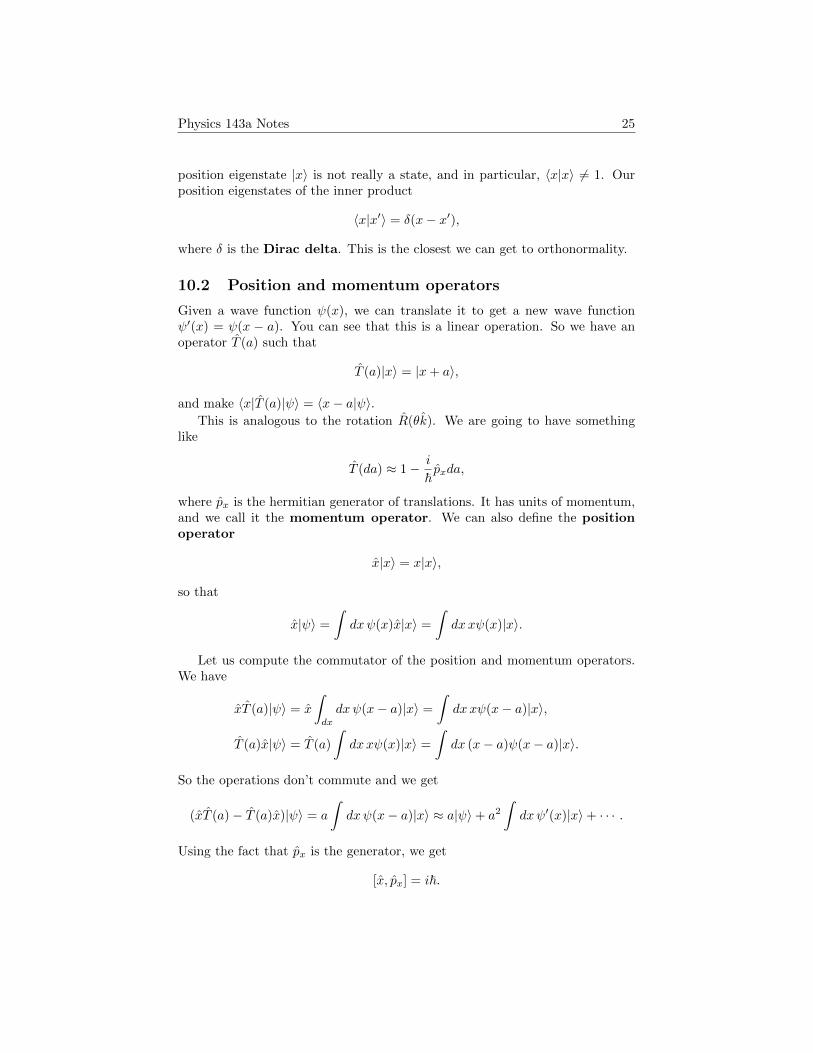
10.2 Position and momentum operators
Given a wave function ψ(x), we can translate it to get a new wave functionψ′(x) = ψ(x − a). You can see that this is a linear operation. So we have anoperator T (a) such that
T (a)|x〉 = |x+ a〉,
and make 〈x|T (a)|ψ〉 = 〈x− a|ψ〉.This is analogous to the rotation R(θk). We are going to have something
like
T (da) ≈ 1− i
~pxda,
where px is the hermitian generator of translations. It has units of momentum,and we call it the momentum operator. We can also define the positionoperator
x|x〉 = x|x〉,
so that
x|ψ〉 =
∫dxψ(x)x|x〉 =
∫dxxψ(x)|x〉.
Let us compute the commutator of the position and momentum operators.We have
xT (a)|ψ〉 = x
∫dx
dxψ(x− a)|x〉 =
∫dxxψ(x− a)|x〉,
T (a)x|ψ〉 = T (a)
∫dxxψ(x)|x〉 =
∫dx (x− a)ψ(x− a)|x〉.
So the operations don’t commute and we get
(xT (a)− T (a)x)|ψ〉 = a
∫dxψ(x− a)|x〉 ≈ a|ψ〉+ a2
∫dxψ′(x)|x〉+ · · · .
Using the fact that px is the generator, we get
[x, px] = i~.

Physics 143a Notes 26
The uncertainty principle implies that
(∆x)(∆px) ≥ ~2,
which is called Heisenberg’s uncertainty principle.Still we haven’t talked about what the momentum operator actually does.
This can be computed as
T (∆x)|ψ〉 =(
1− i
~px∆x
)|ψ〉 =
∫dxψ(x−∆x)|x〉 ≈ |ψ〉 −∆x
∫dxψ′(x)|x〉.
So we get
px|ψ〉 = −i~∫dxdψ(x)
dx|x〉.
That is, momentum operators act by taking derivatives.Let us find eigenstates of momentum. We have −i~(dψ/dx) = pψ(x), and
so ψ(x) = eipx/~. These are called plane waves. These are not normalizablejust like the position eigenstates |x〉. However we still have
〈p|p′〉 = δ(p− p′), 〈x|p〉 = ψp(x) =1√2π~
eipx/~.
For a nontrivial particle, the Hamiltonian is given by
H =1
2mp2x + V (x).
Then |ψ(t)〉 obeys the Schrodinger equation. Since this does not have explicittime dependence,
d
dt〈x〉 =
i
~〈ψ|[H, x]|ψ〉 =
1
m〈px〉.

Physics 143a Notes 27
11 March 2, 2017
We defined the momentum and position operators, each with eigenstates |p〉and |x〉. The relation between them are
〈x|x′〉 = δ(x− x′), 〈p|p′〉 = δ(p− p′), 〈x|p〉 =1√2π~
eipx/~.
11.1 Base change between position and momentum
We know that |x〉 states are a basis, and any state can be written as
|ψ〉 =
∫dxψ(x)|x〉.
The states |p〉 also is a basis, and thus we should be able to always write
|ψ〉 =
∫dp ψ(p)|p〉.
To change basis, we have
ψ(p) = 〈p|ψ〉 =
∫dx 〈p|x〉〈x|ψ〉 =
∫dx
e−ipx/~√2π~
ψ(x).
The inverse transform will be given by
ψ(x) =
∫dpe+ipx/~√
2π~ψ(p).
That is, basis change is given by a Fourier transform.Note that when we look at |x〉 in the momentum basis, the wave function is
given by
ψx(p) =1√2π~
e−ipx/~.
So x|p〉 is given by the wave function
xψx(p) = i~∂
∂pψx(p).
That is, x looks like i~(∂/∂p) in the |p〉-basis.
11.2 Gaussian wave packet
There is a Gaussian wave packet given by the formula
ψ(x) =1
π1/4a1/2e−x
2/2a2 ,

Physics 143a Notes 28
for some real constant a. This satisfies∫dx|ψ(x)|2 = 1. Given this function,
we can compute 〈x〉 = 0 and
〈x2〉 =
∫dxx2|ψ(x)|2 =
1
2a2.
So ∆x = a/√
2. If you look at the same state in momentum space,
ψ(p) =
∫ ∞−∞
1√2π~
e−ipx/~1
a1/2π1/4e−x
2/2a2
=1
(2~a)1/2π3/4
∫ ∞−∞
dx e−(x−x0)2/2a2e−p2a2/2~2
=a1/2
h1/2π1/4e−p
2a2/2~2
.
This is still a Gaussian form! The width is given by ~/a. Then we can compute〈px〉 = 0 and 〈p2
x〉 = ~2/2a2 and ∆p = ~/(√
2a). We can then calculate
∆x∆p =a√2
~√2a
=~2.
So it satisfies the equality for the Heisenberg uncertainty principle. Gaussianwave packets are minimum-uncertainty states, i.e., has the smallest possiblevalue of ∆x∆p.
If ψ(x) is a minimum-uncertainty state at t = 0, is it still at time t > 0?The answer will necessarily depend on the Hamiltonian. Let us consider thecase of a free particle, H = p2
x/2m. Notice that [H, px] = 0 and so energy andmomentum eigenstates are the same. Then |p〉 has energy Ep = p2/2m.
Now we can compute the time evolution of a free particle. We want to findψ(x, t). We have
ψ(p, 0) =a1/2
~1/2π1/4e−p
2a2/2~2
.
So we get
ψ(p, t) =a1/2
~1/2π1/4e−ip
2t/2m~e−p2a2/2~2
.
Taking the Fourier transform gives
ψ(x, t) =
∫dp
1√2π~
eipx/~e−ip2t/2m~ a1/2
~1/2π1/4e−p
2a2/2~2
∼ exp(− x2
2a2(1− i~t/ma2)
),
and this has uncertainty
∆x =a√2
(1 +
~2t2
m2a4
)1/2
.

Physics 143a Notes 29
12 March 7, 2017
For a free particle, the Hamiltonian is given by H = p2x/2m. This has kinetic
energy but no potential energy. The energy eigenstates are |p〉 and H|p〉 =(p2/2m)|p〉.
12.1 Particle in potential
For a particle in a potential, the Hamiltonian is given by
H =1
2mp2x + V (x)
for a potential function V .Let us solve an actual problem. Consider the potential well
V (x) =
{0 |x| < a/2,
V0 |x| > a/2,
for some V0 > 0 a real number. Then V (x) as an operator is
V (x)|x〉 = V (x)|x〉 =
{0 |x| < a/2
V0|x〉 |x| > a/2.
Clearly position eigenstates are always eigenstates of potential energy and mo-mentum eigenstates are always eigenstates of kinetic energy.
Given |ψ(0)〉 we want to know |ψ(t)〉. In the position basis, the time-dependent Schrodinger equation becomes[
− ~2
2m
∂2
∂x2+ V (x)
]ψ(x, t) = i~
∂
∂tψ(x, t).
To actually solve it, we look at the time-independent Schrodinger equation.We are then trying to solve
− ~2
2m
∂2
∂x2ψ(x) + V (x)ψ(x) = Eψ(x).
There are two regions:{d2
dx2ψ(x) = − 2mE~2 ψ(x), |x| < a/2,
d2
dx2ψ(x) = − 2m(E−V0)~2 ψ(x), |x| > a/2.
The solutions to these equations depend on the signs of the constants.

Physics 143a Notes 30
Consider first the range 0 < E < V0. Then in |x| < a/2 the solution is goingto be oscillating and in |x| > a/2 it is going to be exponential.1 Then
ψ(x) =
A sin kx+B cos kx, |x| < a/2,
Ceqx +De−qx, x > q/2,
F eqx +Ge−qx, x < −q/2,k =
√2mE
~2, q =
√2m(V0 − E)
~2.
Here, the wavefunction must not blow up as |x| → ∞. This shows that C =G = 0.
There are also some boundary conditions at x = ±a/2. We want to requireψ(x) to be continuous. Because we need to be able to take the derivative. Then
A sin(ka/2) +B cos(ka/2) = De−qa/2,
−A sin(ka/2) +B cos(ka/2) = Fe−qa/2.
In this case, we can also impose that dψ/dx is continuous, because d2ψ/dx2 islocally bounded by the equation we are trying to solve. So we get two moreequations. There is also a normalization constraint. That is, we won’t find asolution for all E and get a discrete spectrum.
You can solve the equation, but we are going to simplify it by sending V0 →∞. Then q →∞ and so ψ(x)→ 0 for all |x| > a/2. The equations become
A sin(ka/2) +B cos(ka/2) = 0,
−A sin(ka/2) +B cos(ka/2) = 0.
Because I don’t want A = B = 0, either sin(ka/2) = 0 or cos(ka/2) = 0. Thatmeans k = 0, π/a, 2π/a, 3π/a, . . .. Then
En =~2k2
n
2m=
~2n2π2
2ma2.
The solutions are given by
k1 =π
a, ψ1(x) =
√2
acos(πxa
),
k2 =2π
a, ψ2(x) =
√2
asin(2πx
a
), . . . .
For unbound particles, the eigenstates are going to be joined oscillatingfunctions. They are not normalizable and have a continuous spectrum. Butyou can add (integrate) them together to get normalizable states, like the freeparticle in Gaussian state.
1A general rule is that if E > V (x) the wave function will be locally oscillating and ifE < V (x) the wave function will be locally exponential. In classical mechanics, E < V (x)doesn’t make sense, and this is usually reflected in quantum mechanics by exponential decay.

Physics 143a Notes 31
13 March 9, 2017
For the time-independent Schrodinger equation, E < V gives an oscillatingsolution and E > V gives an exponentially growing or decreasing solution. Thebound solutions are going to have discrete energy, and the oscillating solutionsare going to be a continuum.
13.1 Physical interpretation of oscillating solutions
Although the oscillating states are not normalizable, there is some physics wecan extract from these solutions. Consider a potential given by
V (x) =
{0 x < 0
V0 x ≥ 0.
Let us look at the solutions for 0 < E < V0, i.e., solutions that exponentiallydecay on the right and oscillates on the left. They are going to look like
ψ(x) =
{Aeikx +Beikx x < 0,
Ce−qx x > 0,k =
√2mE
~2, q =
√2m(V0 − E)
~2.
The conditions ψ begin continuous and differentiable at x = 0 give A+B = Cand ikA− ikB = −qC. Then C = (2k/(k + iq))A = (2k/(k − iq))B. From thiswe see that |A| = |B|.
You can solve the similar problem for E > V0 and the answer is going tohave a slightly different form:
ψ(x) =
{Aeikx +Be−ikx x < 0,
Ceik′x +De−ik
′x x > 0,k =
√2mE
~2, k′ =
√2m(E − V0)
~2.
Let us just look at the solutions with D = 0. Then continuity of ψ and ψ′ againgives C = (2k/(k + k′))A = (2k/(k − k′))B. Here we observe |A| 6= |B|.
The time evolution of the energy eigenstates are given by
ψ(x, t) = e−iEt/~ψ(x).
Then eikx becomes ei(kx−ωt) where ω = E/~. This is a right moving wave, andlikewise e−ikx is a left moving wave.
In the case of E < V0, the interpretation is that there is stream of particlesgoing in the left direction and another stream of particles with same intensitygoing in the right direction, on the x < 0 region. From the classical perspective,you can think of these particle bouncing back from the potential wall.
Now what is happening for E > V0? We can think of A as particles that aremoving to the right. Then B are the particles that bounces back, and C are theparticles that get through.

Physics 143a Notes 32
There is a conservation law related to the conservation of the particles inthe interpretation. We define the probability current as
jx =~
2πi
(ψ∗∂ψ
∂x− ψ∂ψ
∗
∂x
).
If we write the probability density ρ = ψ∗ψ, then there is the conservation law
∂ρ
∂t+
∂
∂xjx = 0.
In the case of ψ = Aei(kx−ωt) +Bei(−kx−ωt), the current is given by
jx =~km
(|A|2 − |B|2
).
This ~k/m can be thought of as velocity and |A|2 can be thought of as right-moving flux and |B|2 as left-moving flux.
This let us define reflection/transmission coefficients. In the case ofE < V0, we have
jx =
{~km (|A|2 − |B|2) = 0 x < 0,
0 x > 0.
The reflection coefficient is given by
R =|B|2
|A|2= 1.
For the E > V0 case, the currents are
jtrans =~k′
m|C|2, jinc =
~km|A|2, jref =
~km|B|2.
Then the reflection and transmission coefficients are
R =jref
jinc=(k − k′k + k′
)2
, T =jtrans
jinc=
4kk′
(k + k′)2, R+ T = 1.
Consider potential that looks like
V (x) =
{0 |x| > a/2,
V0 |x| ≤ a/2.
If we send things from the left, there is something coming out from the right,unlike the classical case. This is called tunneling. I will not compute this, butthe result is
T =jtrans
jinc=
1
1 + k2+q2
2kq sinh2(qa)≈( 4kq
k2 + q2
)e−2qa.
The price you pay for tunneling is the exponential factor e−2qa.

Physics 143a Notes 33
13.2 Ladder operators
The Hamiltonian for the harmonic oscillator is given by
H =p2x
2m+
1
2mω2x2.
We have a useful fact that [x, px] = i~. In the case of J , we used the trick ofdefining J± = Jx ± iJy and showed that [Jz, J±] = ±~J±.
We are going to use a similar trick and find ladder operators a and a†
such that
[H, a] = −~ωa, [H, a†] = ~ωa†.
Note that [x2, px] is proportional to x and [p2x, x] is proportional to px. So we
can define
a =
√mω
2~
(x+
i
mωpx
).
Then [H, a] = −~ωa and [a, a†] = 1 and H = a†a+ 12~ω.
Physics 143a Notes 34
14 March 21, 2017
There is a midterm on March 28, which will cover mostly chapters 3, 4, 6, anda little bit of 1, 2, 7.
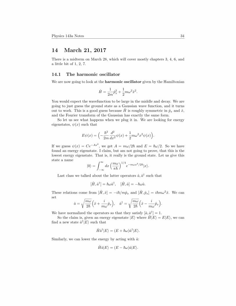
14.1 The harmonic oscillator
We are now going to look at the harmonic oscillator given by the Hamiltonian
H =1
2mp2x +
1
2mω2x2.
You would expect the wavefunction to be large in the middle and decay. We aregoing to just guess the ground state as a Gaussian wave function, and it turnsout to work. This is a good guess because H is roughly symmetric in px and x,and the Fourier transform of the Gaussian has exactly the same form.
So let us see what happens when we plug it in. We are looking for energyeigenstates, ψ(x) such that
Eψ(x) =(− ~2
2m
d2
dx2ψ(x) +
1
2mω2x2ψ(x)
).
If we guess ψ(x) = Ce−Ax2
, we get A = mω/2~ and E = ~ω/2. So we havefound an energy eigenstate. I claim, but am not going to prove, that this is thelowest energy eigenstate. That is, it really is the ground state. Let us give thisstate a name
|0〉 =
∫ ∞−∞
dx(mωπ~
)1/4
e−mωx2/2~|x〉.
Last class we talked about the latter operators a, a† such that
[H, a†] = ~ωa†, [H, a] = −~ωa.
These relations come from [H, x] = −i~/mpx and [H, px] = i~mω2x. We canset
a =
√mω
2~
(x+
i
mωpx
), a† =
√mω
2~
(x− i
mωpx
).
We have normalized the operators so that they satisfy [a, a†] = 1.So the claim is, given an energy eigenstate |E〉 where H|E〉 = E|E〉, we can
find a new state a†|E〉 such that
Ha†|E〉 = (E + ~ω)a†|E〉.
Similarly, we can lower the energy by acting with a:
Ha|E〉 = (E − ~ω)a|E〉.
Physics 143a Notes 35
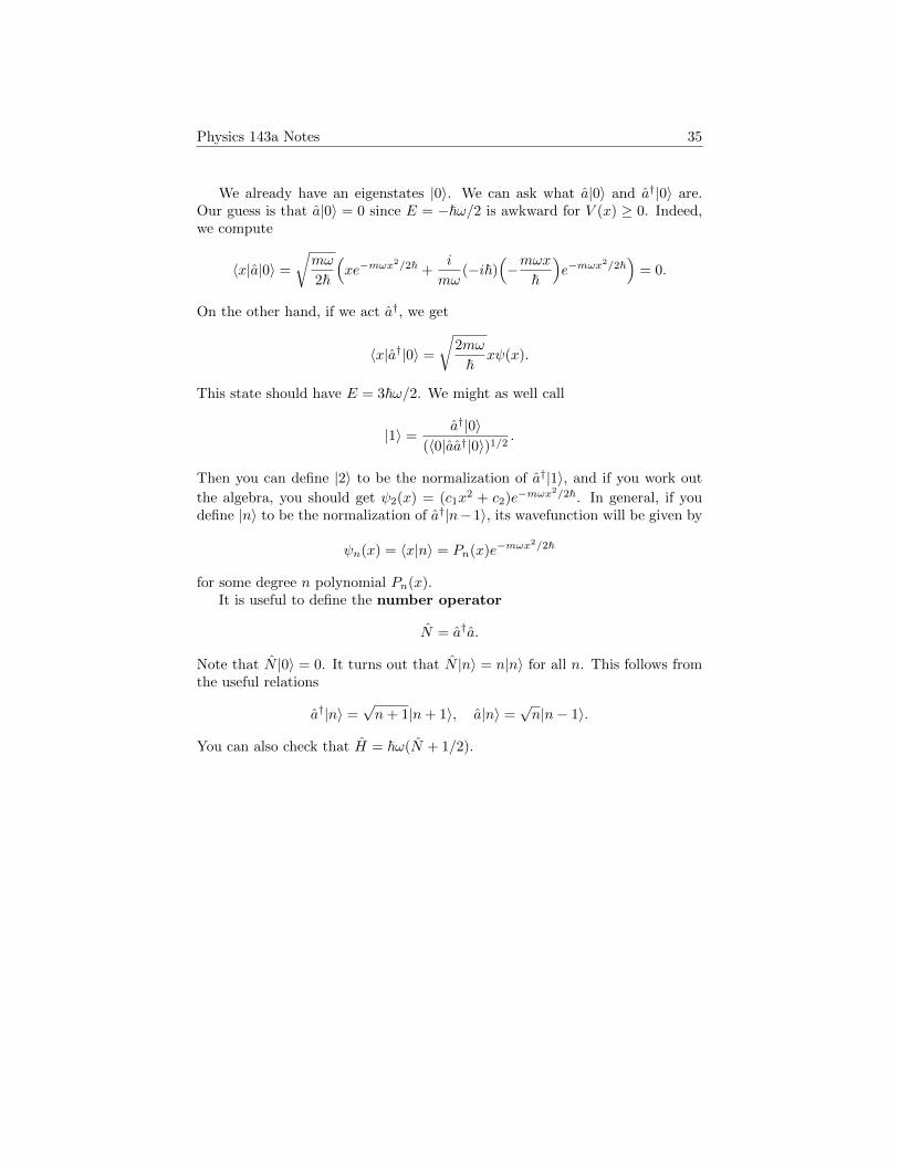
We already have an eigenstates |0〉. We can ask what a|0〉 and a†|0〉 are.Our guess is that a|0〉 = 0 since E = −~ω/2 is awkward for V (x) ≥ 0. Indeed,we compute
〈x|a|0〉 =
√mω
2~
(xe−mωx
2/2~ +i
mω(−i~)
(−mωx
~
)e−mωx
2/2~)
= 0.
On the other hand, if we act a†, we get
〈x|a†|0〉 =
√2mω
~xψ(x).
This state should have E = 3~ω/2. We might as well call
|1〉 =a†|0〉
(〈0|aa†|0〉)1/2.
Then you can define |2〉 to be the normalization of a†|1〉, and if you work out
the algebra, you should get ψ2(x) = (c1x2 + c2)e−mωx
2/2~. In general, if youdefine |n〉 to be the normalization of a†|n−1〉, its wavefunction will be given by
ψn(x) = 〈x|n〉 = Pn(x)e−mωx2/2~
for some degree n polynomial Pn(x).It is useful to define the number operator
N = a†a.
Note that N |0〉 = 0. It turns out that N |n〉 = n|n〉 for all n. This follows fromthe useful relations
a†|n〉 =√n+ 1|n+ 1〉, a|n〉 =
√n|n− 1〉.
You can also check that H = ~ω(N + 1/2).

Physics 143a Notes 36
15 March 23, 2017
This lecture was taught by Prateek Agrawal. We defined the raising operator
a† =
√mω
2~
(x− i
mωp),
and applying this operator gives higher eigenstates by a† =√n+ 1|n+ 1〉. The
wave functions have the pattern of ψn(−x) = (−1)nψn(x), and
ψn(x) = Pn(x)e−mω2x2/2~
for some degree n polynomial Pn(x). We can express this using the parityoperator
Π|n〉 = (−1)n|n〉.
This commutes with the Hamiltonian: [H, Π] = 0.
15.1 Coherent states
We want to find eigenfunctions of the lowering operator. Recall that if we setup a Gaussian wave function with a free particle, it spreads out. But for theHarmonic oscillator, this does not happen.
For n 6= 0, the states |n〉 are not minimum uncertainty states. Indeed,Gaussian wave functions are the only minimum uncertainty states. We wantour wave function to take the form of a Gaussian wave packet for any giventime. That is,
ψ(x, t) = Ceiφ(t)e−(x−x0(t))2/2a2(t)eip0(t)x/~.
Now we want this wave function to satisfy the Hamiltonian equation. Thenit has to satisfy the equations
d〈px〉dt
= −⟨∂V∂x
⟩= −mω2〈x〉, d〈x〉
dt=〈px〉m
.
Note that 〈x〉 = x0(t) and 〈px〉 = p0(t). This is then just the classical harmonicoscillator. It can be written as
x0(t) = A sin(ωt+ φ).
Using this, you can then compute a(t) =√~/mω and φ(t) = −ωt/2−p0(t)x0(t)/2~.
If you write out, we get
ψ(x, t) =(mωπ~
)1/4
e−i2 (ωt+
p0(t)x0(t)~ )e−mω(x−x0(t))2/2~eip0(t)x/~.
These have ∆x = a/√
2 and ∆x∆p = ~/2 at any time.
Physics 143a Notes 37
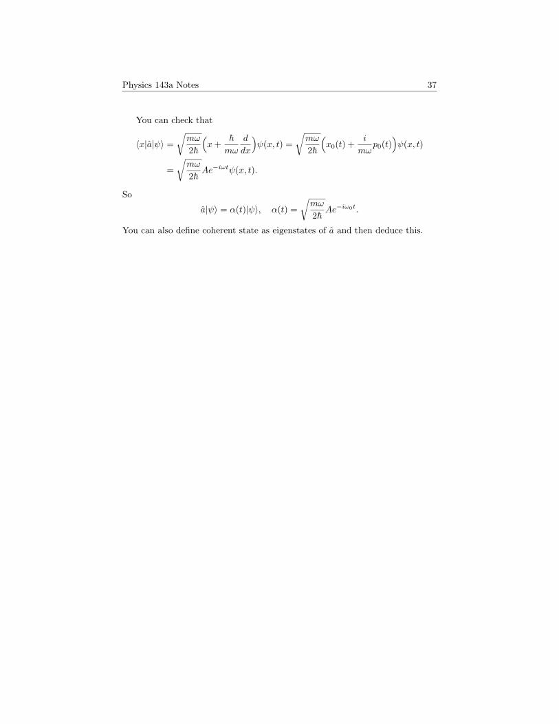
You can check that
〈x|a|ψ〉 =
√mω
2~
(x+
~mω
d
dx
)ψ(x, t) =
√mω
2~
(x0(t) +
i
mωp0(t)
)ψ(x, t)
=
√mω
2~Ae−iωtψ(x, t).
So
a|ψ〉 = α(t)|ψ〉, α(t) =
√mω
2~Ae−iω0t.
You can also define coherent state as eigenstates of a and then deduce this.

Physics 143a Notes 38
16 March 30, 2017
Coherent states are eigenstates of the lowering operator:
a|α〉 = α|α〉.
Here a is not hermitian and so |α〉 is not associated with a measurement. Ithink this is not a good motivation for coherent states.
The other way to characterize them is that they are minimum uncertaintystates. The ground state |0〉 is a Gaussian wave packet and so it is a minimumuncertainty state. But for |n〉, it is not a minimum uncertainty state. It isa special fact of the harmonic oscillator that there are minimum uncertaintystates that remain so under time evolution.
The wavefunctions of coherent states are given by
ψ(x, t) =(mωπ~
)1/4
e−i2 [ωt+ 1
~p0(t)x0(t)]e−12~mω(x−x0(t))2e
1~ ip0(t)x,
where x0(t) and p0(t) solve the classical equation of motion.If we look at |n〉 for n � 1, it looks complicated but it stays the same as
time evolves, up to a phase. If we take a coherent state, it looks like a Gaussian,but it oscillates as time evolves. So it is more closer to classical physics. Thisis used in experiments a lot because they have minimum uncertain.
Given a coherent state |α〉, the probability of finding energy En = ~ω(n+ 12 )
is
Pn = |〈n|α〉|2 =∣∣∣e− 1
2 |α|2 αn√
n!
∣∣∣2 = e−|α|2 |α|2n
n!.
Because 〈N〉 = 〈a†a〉 = |α|2, we can also write
Pn = e−〈N〉|N |n
n!.
This is a Poisson distribution. If 〈N〉 � 1, then the mean is 〈N〉 and itsstandard deviation is
√〈N〉. This means that states with higher energy are
more well explained by classical physics.
16.1 Particles in three dimension
We are now going to look at particles in higher dimension. There are differ-ent coordinates we can work with. In the future, we are going to solve theSchrodinger equation for the hydrogen atom. It is natural to work in sphericalcoordinates there.
In 3-dimension, there are going to be position operators in 3-dimensions: x,y, z. We assume that they commute with each other.
[x, y] = [y, z] = [z, x] = 0.
This allows us to talk about simultaneous eigenstates |x, y, z〉 such that
x|x, y, z〉 = x|x, y, z〉, y|x, y, z〉 = y|x, y, z〉, z|x, y, z〉.

Physics 143a Notes 39
Just as we did in the 1-dimensional problem, we can write a general state as
|ψ〉 =
∫ ∞−∞
dx
∫ ∞−∞
dy
∫ ∞−∞
dz ψ(x, y, z)|x, y, z〉 =
∫d3r ψ(~r)|~r〉.
A stated is normalized if ∫d3~r|ψ(r)|2 = 1.
We also chose
〈x, y, z|x′, y′, z′〉 = δ(x− x′)δ(y − y′)δ(z − z′).
We are going to write this as
〈~r|~r′〉 = δ3(~r − ~r′).
Define the (unitary) translation operator as
T (~a)|~r〉 = |~r + ~a〉.
Translations in different direction are supposed to commute. For instance, weshould have T (axi)T (ay j) = T (ay j)T (axi).
There are the (hermitian) momentum operators px, py, pz that generate thetranslation operators:
T (axi) = e−iaxpx/~.
For a general vector a, we can also define
T (~a) = e−i~p·~a/~, ~p = (py, py, pz).
This is well-defined because px, py, pz pairwise commute.In the case of 1-dimension, we had
[x, px] = i~, [y, py] = i~, [z, pz] = i~.
We can also ask about commutators with mixed directions. If I translate inthe y-direction and then act by x, this is the same as acting by x and thentranslating. So x and py should commute. So to summarize,
[xi, py] = i~δij .
If we act on a wavefunction, the momentum operators are going to look like
px 7→ −i~∂
∂x, py 7→ −i~
∂
∂y, pz 7→ −i~
∂
∂z.
Also the momentum eigenstates are going to look like
〈~r|~p〉 =1
(2π~)3/2ei~p·~r/~ = 〈x|px〉〈y|py〉〈z|pz〉.

Physics 143a Notes 40
16.2 Multiparticle states
Eventually we want to look at the hydrogen atom, and this is a system of twoparticles. If we have two particles, the position eigenstates has to contain thedata of the position of both particles. So we can write this eigenstate as
|~r1, ~r2〉 = |~r1〉1 ⊗ |~r2〉2 = |~r1〉1|~r2〉2.
If I have a general vector space V consisting of |ψ〉 =∑ni=1 ci|vi〉 then its
tensor product V ⊗ V consists of
|ψ〉 =
n∑i=1
n∑j=1
cij |vi〉1|vj〉2 =
n∑i=1
cij |vi, vj〉.
We will use both notations.

Physics 143a Notes 41
17 April 4, 2017
I want to resume what we are talking last time, which is states of two particles.We can label the position eigenstates as
|~r1, ~r2〉 = |~r1〉1|~r2〉2.
There are position operators that act as
x1|~r1, ~r2〉 = x1|~r1, ~r2〉, x2|~r1, ~r2〉 = x2|~r1, ~r2〉, y1|~r1, ~r2〉 = y1|~r1, ~r2〉, · · · .
There are also translation operators
T1(~a)|~r1, ~r2〉 = |~r1 + ~a,~r2〉, T2(~a) = |~r1, ~r2〉 = |~r1, ~r2 + ~a〉.
We can talk about their generators,
T1(~a) = e−i~p1·~a/~, T2(~a) = e−i~p2·~a/~,
where ~p1 and ~p2 are hermitian momentum operator. We can also talk about thetotal momentum,
~P = ~p1 + ~p2, Px = p1x + p2x, · · · .
Generally, a 2-particle Hamiltonian is going to be given by
H =1
2m1~p2
1 +1
2~p2
2 + V (~r1, ~r2).
We are interested in the special case of a central potential, given by V (~r1, ~r2) =V (|~r1 − ~r2|). For instance, in the case of the hydrogen atom, the Coulombpotential is given by
V (~r1, ~r2) = −e2/|~r1 − ~r2|.
Here V (~r1, ~r2) defines an operator
〈~r′1, ~r′2|V (~r1, ~r2)|ψ〉 = ψ(~r′1, ~r′2)V (~r′1, ~r
′2).
17.1 Center-of-mass frame
Our goal now is to go to the center-of-mass frame to simplify the problem. Weobserve that [H, ~p1] 6= 0 because [V (~r1, ~r2), ~p1] 6= 0 if V has any ~r1 dependence.
Likewise [H, ~p2] 6= 0 if V has any ~r2-dependence. However,
[H, ~P ] = 0
if V is translation invariant, i.e., V (~r1, ~r2) = V (~r1 − ~r2). This is because T (~a)
commutes with H. So we can talk about states |E, ~P 〉 because [H, ~P ] = 0 justas we have talked about states |j,m〉.
Physics 143a Notes 42
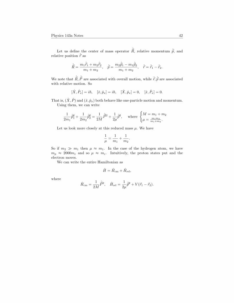
Let us define the center of mass operator ~R, relative momentum ~p, andrelative position ~r as
~R =m1~r1 +m2~r2
m1 +m2, ~p =
m2~p1 −m1~p2
m1 +m2, ~r = ~r1 − ~r2.
We note that ~R, ~P are associated with overall motion, while ~r, ~p are associatedwith relative motion. So
[X, Px] = i~, [x, px] = i~, [X, px] = 0, [x, Px] = 0.
That is, (X, P ) and (x, px) both behave like one-particle motion and momentum.Using them, we can write
1
2m1~p2
1 +1
2m2~p2
2 =1
2M~P 2 +
1
2µ~p2, where
{M = m1 +m2
µ = m1m2
m1+m2.
Let us look more closely at this reduced mass µ. We have
1
µ=
1
m1+
1
m2.
So if m2 � m1 then µ ≈ m1. In the case of the hydrogen atom, we havemp ≈ 2000me and so µ ≈ me. Intuitively, the proton states put and theelectron moves.
We can write the entire Hamiltonian as
H = Hcm + Hrel,
where
Hcm =1
2M~P 2, Hrel =
1
2µ~p2 + V (~r1 − ~r2).

Physics 143a Notes 43
18 April 6, 2017
Today we are going to talk about orbital angular momentum and spin.
18.1 Orbital angular momentum
Recall that the angular momentum algebra
[Jx, Jy] = i~Jz
followed from R ∼ e−iJθ/~ and properties of rotations. We introduce operatorsfor orbital angular momentum
~L = ~r × ~p, Lx = ypz − zpy, Ly = zpx − xpz, Lz = xpy − ypx.
If we compute the commutator between the two angular momentum opera-tors, we get
[Lx, Ly] = [ypx − zpy, zpx − xpz]= [ypz, zpx]− [zpy, zpx]− [ypz, xpz] + [zpy, xpz]
= ypx[pz, z] + xpy[z, pz] = i~Lz.
There are also the commutation relations
[Lx, y] = i~x, [Lx, x] = 0, [Lx, py] = i~pz, [Lx, px] = 0.
We also have [Lx, ~r2] = 0 and so
[~L, V (~r)] = 0
when V is a central potential. Likewise, [~L, ~p2] = 0. The conclusion is that,
[~L, H] = 0, if H =1
2µ~p2 + V (|~r|).
This is ignoring spin. If there is spin, the conserved quantity is going to be
~J = ~L+ ~S.
Because H and ~L commute, we can find a basis of simultaneous eigenstates.If you remember the case the spin system, we also had another commuting
operator ~J2. The analogue of this is
[~L2, Lz] = 0, [~L2, H] = 0.
So we can name the simultaneous eigenstates of L2 and Lz as
~L2|l,m〉 = l(l + 1)~2|l,m〉, Lz|l,m〉 = m~|l,m〉,
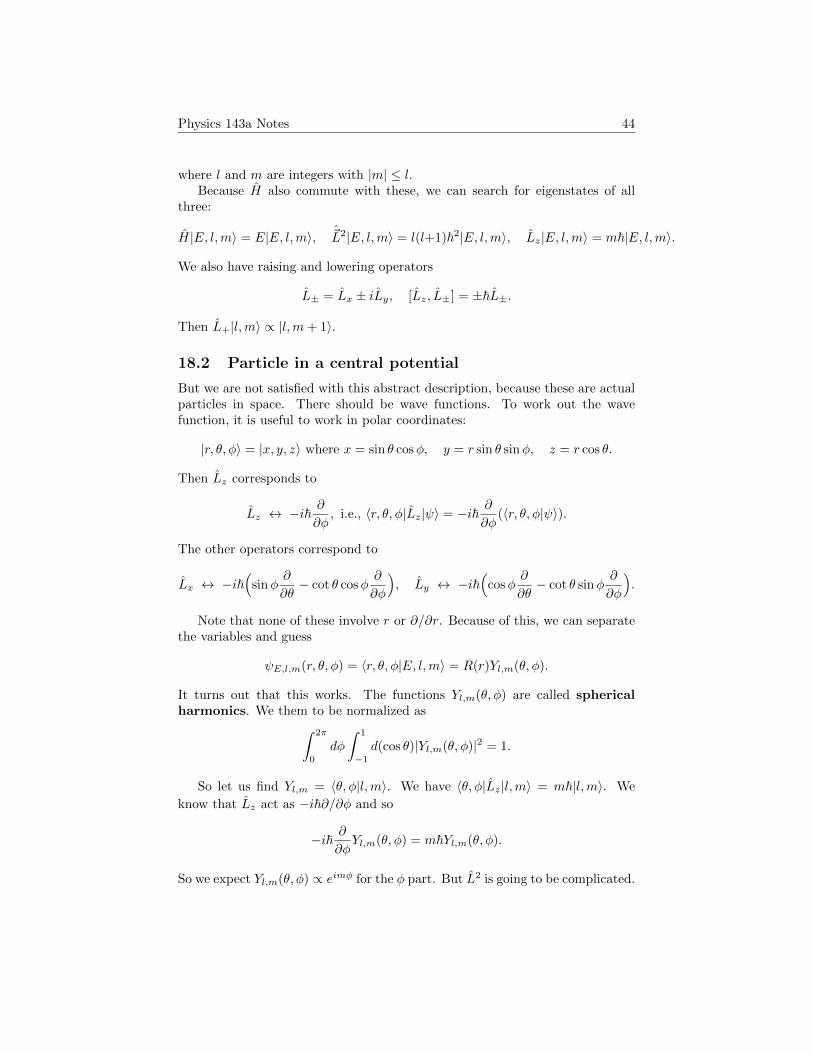
Physics 143a Notes 44
where l and m are integers with |m| ≤ l.Because H also commute with these, we can search for eigenstates of all
three:
H|E, l,m〉 = E|E, l,m〉, ~L2|E, l,m〉 = l(l+1)~2|E, l,m〉, Lz|E, l,m〉 = m~|E, l,m〉.
We also have raising and lowering operators
L± = Lx ± iLy, [Lz, L±] = ±~L±.
Then L+|l,m〉 ∝ |l,m+ 1〉.
18.2 Particle in a central potential
But we are not satisfied with this abstract description, because these are actualparticles in space. There should be wave functions. To work out the wavefunction, it is useful to work in polar coordinates:
|r, θ, φ〉 = |x, y, z〉 where x = sin θ cosφ, y = r sin θ sinφ, z = r cos θ.
Then Lz corresponds to
Lz ↔ −i~ ∂
∂φ, i.e., 〈r, θ, φ|Lz|ψ〉 = −i~ ∂
∂φ(〈r, θ, φ|ψ〉).
The other operators correspond to
Lx ↔ −i~(
sinφ∂
∂θ− cot θ cosφ
∂
∂φ
), Ly ↔ −i~
(cosφ
∂
∂θ− cot θ sinφ
∂
∂φ
).
Note that none of these involve r or ∂/∂r. Because of this, we can separatethe variables and guess
ψE,l,m(r, θ, φ) = 〈r, θ, φ|E, l,m〉 = R(r)Yl,m(θ, φ).
It turns out that this works. The functions Yl,m(θ, φ) are called sphericalharmonics. We them to be normalized as∫ 2π
0
dφ
∫ 1
−1
d(cos θ)|Yl,m(θ, φ)|2 = 1.
So let us find Yl,m = 〈θ, φ|l,m〉. We have 〈θ, φ|Lz|l,m〉 = m~|l,m〉. We
know that Lz act as −i~∂/∂φ and so
−i~ ∂
∂φYl,m(θ, φ) = m~Yl,m(θ, φ).
So we expect Yl,m(θ, φ) ∝ eimφ for the φ part. But L2 is going to be complicated.

Physics 143a Notes 45
Instead of expanding everything out, we use L+|l, l〉 = 0. We can write
L± = Lz ± iLy = ±i~e±iφ(±i ∂∂φ− cot θ
∂
∂φ
).
Using this, we can write ( ∂∂θ− l cot θ
)Yll(θ, φ) = 0
and so Yll(θ, φ) = cll(sin θ)leilφ.

Physics 143a Notes 46
19 April 11, 2017
We were studying a particle in a central potential
H =p2
2µ+ V (|~r|).
This gave rotationally invariant operators ~L2 and Lz that commute with H.
Our strategy is to look for states |E, `,m〉 which are eigenstates of H, ~L2, Lzsimultaneously. We are also going go work in polar coordinates. Because p2
decomposes into a radial part and an angular part, we can look for wavefunctions
〈r, θ, φ|E, `,m〉 = R`(r)Y`m(θ, ϕ).
Here we want
~L2|`,m〉 = `(`+ 1)~2|`,m〉, Lz|`,m〉 = m~|`,m〉.
In particular, Y`,m(θ, φ) are universal for all central potentials but R`(r) dependson V (|r|). So these functions are going useful for any central potentials.
Our goal is to solve this for the Coulomb potential
V (r) = −e2
r, where e2 ≈ 1
137~c.
19.1 Spherical harmonics
Last time we have worked out the operators
Lz → −i~∂
∂φ, L± → −i~e±iφ
(±i ∂∂θ− cot θ
∂
∂φ
).
From the first equation, we expect Y`,m(θ, φ) ∝ eimφ. Then we would expect
L+|`, `〉 = 0 and so (∂/∂θ − ` cot θ)Y`,`(θ, φ) = 0. This gives
Y`,`(θ, φ) = c`,`(sin θ)`ei`φ =
(−1)`
2``!
√(2`+ 1)!
4πei`φ(sin θ)`.
Here, note that if we want Y`,m(θ, φ) ∝ eimφ, then
Y`,m(θ, φ+ 2π) ∝ eim(φ+2π) =
{eimφ if m ∈ Z−eimφ if m ∈ Z + 1
2 .
Then if we want this to be a single-valued wave function, we would need `,m ∈ Z.But for spin particles, we did not require this because spin are not rotations.
Anyways, once we know |`,m〉, we can compute |`,m − 1〉 by applying L−and then normalizing it:
Y`,m−1(θ, φ) =1√
`(`+ 1)−m(m− 1)
1
~(−i~e−iφ)
(−i ∂∂θ− cot θ
∂
∂φ
)Y`,m(θ, φ).

Physics 143a Notes 47
The operator ~L2 is given by
~L2 = −~2[ 1
sin θ
∂
∂θ
(sin θ
∂ψ
∂θ
)+
1
sin2 θ
∂2ψ
∂φ2
].
Even though we have not solved the eigenvalue equation for ~L2, it is auto-matically going to be satisfied because we have used the raising and lowering
operators L±. You can explicitly check ~L2|`,m〉 = `(`+ 1)~2|`,m〉 if you want.
19.2 Boundary condition for the radial function
To compute the radial functions, we now actually need to solve the time-independent Schrodinger equation:⟨
r, θ, φ∣∣∣( p2
2µ+ V (|r|)
)∣∣∣E, `,m⟩ = EψE,`,m(r, θ, φ) = ERE,`(r)Y`,m(θ, φ).
Then the equation we want to solve is[− ~2
2µ
( ∂2
∂r2+
2
r
∂
∂r
)+
1
2µr2`(`+ 1)~2 + V (r)
]RE,`(r) = ERE,`(r)
after canceling out the angular part.The equation is getting is nicer but it is still ugly to solve. The trick is to
convert (∂2/∂r2 + (2/r)∂/∂r)R into a nice factor (∂2/∂r2)u. Note that
∂2
∂r2(rR) = r
( ∂2
∂r2+
2
r
∂
∂r
)R.
So uE,`(r) = rRE,`(r) satisfies the equation[− ~2
2µ
d2
dr2+`(`+ 1)~2
2µr2+ V (r)
]uE,`(r) = EuE,`(r).
If we can solve this for uE,`(r) for V (r) = −e2/r, we will have solved thehydrogen atom. This now just looks like a one-dimensional particle in a potentialwell, with
Veff(r) =`(`+ 1)~2
2µr2− Z e
2
r.
We’re looking for bound states with E < 0, since plane wave-like solutionsexist when E > 0. We are going to impose normalizability:∫
d3r|ψ(r)|2 = 1 = c
∫r2drR(r)2.
So we want r2R(r)2 to not grow too fast. The decay r2R2 ∼ r−1−ε is enough.

Physics 143a Notes 48
20 April 13, 2017
We are looking for solutions to ψE,`,m(r, θ, φ) = RE,`(r)Y`,m(θ, φ). If we defineuE,`(r) = rRE,`(r), then
− ~2
2µ
d2
dr2uE,`(r) + Veff(r)uE,`(r) = EuE,`(r),
where
Veff(r) = −Z e2
r+`(`+ 1)~2
2µr2.
The boundary condition for large r was that∫drr2|R(r)|2 < ∞. For small
r, we have (assuming that ` > 0)∣∣∣`(`+ 1)~2
2µr2
∣∣∣� ∣∣∣−Z e2
r
∣∣∣.Then the centrifugal term dominates and the equation looks like
− d2
dr2uE,`(r) +
`(`+ 1)
r2uE,`(r) ≈ E
2µ
~2uE,`(r).
If we guess that the leading term is uE,`(r) ∝ r−α, then
[−α(α+ 1)u−α−2 + · · · ] + [`(`+ 1)r−α−2 + · · · ] ≈ E 2µ
~2r−α.
So we get α(α+ 1) = `(`+ 1) and so either α = ` or α = −(`+ 1). But we againhave
∫drr2|R(r)|2 =
∫dr|u|2. This shows that the solution for α = ` grows
too fast and so α = −(`+ 1). So for ` ≥ 1, we want uE,`(r) ∼ r`+1 as r → 0.The case ` = 0 is a bit subtle. We only have the Coulomb term and so
− ~2
2µ
d2
dr2u(r)− Z e
2
ru(r) = Eu(r).
If we assume u(r) = r−α + · · · then the equation becomes
− ~2
2µα(α+ 1)r−α−2 + · · · − Ze2r−α−1 + · · · = Er−α + · · · .
So α = 0 or α = −1. Both of u ∼ r0 and u ∼ r1 satisfies normalizability.The “correct” choice is to pick u ∼ r1 and R ∼ const. The textbook gives
two reasons for this:
(1) problem 10.1: 〈pr〉 is not real if R ∼ r−1.
(2) Because ∇2r−1 = δ3(~r), and so the solution with R ∼ r−1 is really solvingthe Schrodinger equation with
V (r) = −Z e2
r+ bδ3(~r).

Physics 143a Notes 49
Really, it is not clear whether the interaction between the proton andthe electron is just −Ze2/r or −Ze2/r + bδ3(~r). This is an empiricalfact that in our universe, b is really small. So RE,`(r) = const is a goodapproximation.
Anyways, in both ` = 0 and ` ≥ 1, we have the boundary conditionsRE,`(r) ∼ r`as r → 0.
20.1 Radial function for the Coulomb potential
Now we really need to solve the equation. First choose units of length based on
ρ = κEr, E = −~2κ2E
2µ.
Note that this is possible since E < 0. The Schrodinger equation then becomes
− d2
dρ2uE,`(ρ) +
(−ξEr
+`(`+ 1)
ρ2
)uE,`(ρ) = −uE,`(ρ),
where ξE = 2µZe2/(κE~2).We know that the behavior of uE,`(ρ) as ρ→ 0 is like ρ`+1 and the behavior
as ρ→∞ is something like exponential decay. So we make an ansatz
uE,`(ρ) = ρ`+1e−ρFE,`(ρ).
This can be expected to go to a constant as ρ→ 0, and is somewhat controlledas ρ→∞.
Plugging this in, we get
d2FE,`dρ2
− 2(
1− `+ 1
ρ
)dFE,`dρ
+(ξE − 2`− 2
ρ
)FE,`(ρ) = 0.
If we try a series solution F (ρ) =∑∞n=0 anρ
n where a0 6= 0, we get
∞∑n=0
[ann(n− 1)ρn−2 − 2nanρn−1 + 2(`+ 1)nanρ
n−2 + (ξE − 2`− 2)anρn−1] = 0.
There are no ρ−2 terms, and ρ−1 terms give
(ξE − 2`− 2)a0 + 2(`+ 1)a1 = 0 and so a2 =2(`+ 1)− ξE
2(`+ 1)a0.
Next, ρ0 terms give
2a2 − 2a1 + 4(`+ 1)a2 + (ξE − 2`− 2)a1 = 0 and so a2 =(2`+ 3− ξE)a1
4`+ 6.
In general, we are going to see
an+1 = an(−ξE + 2n+ 2`+ 2)
(n+ 2`+ 2)(n+ 1).
Physics 143a Notes 50
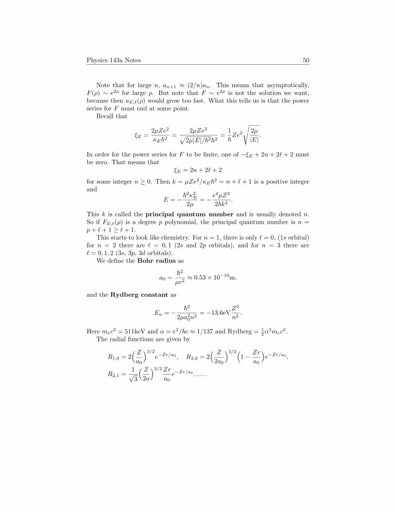
Note that for large n, an+1 ≈ (2/n)an. This means that asymptotically,F (ρ) ∼ e2ρ for large ρ. But note that F ∼ e2ρ is not the solution we want,because then uE,`(ρ) would grow too fast. What this tells us is that the powerseries for F must end at some point.
Recall that
ξE =2µZe2
κE~2=
2µZe2√2µ|E|/~2~2
=1
~Ze2
√2µ
|E|.
In order for the power series for F to be finite, one of −ξE + 2n+ 2`+ 2 mustbe zero. That means that
ξE = 2n+ 2`+ 2
for some integer n ≥ 0. Then k = µZe2/κE~2 = n+ `+ 1 is a positive integerand
E = −~2κ2E
2µ= −e
4µZ2
2~k2.
This k is called the principal quantum number and is usually denoted n.So if FE,`(ρ) is a degree p polynomial, the principal quantum number is n =p+ `+ 1 ≥ `+ 1.
This starts to look like chemistry. For n = 1, there is only ` = 0, (1s orbital)for n = 2 there are ` = 0, 1 (2s and 2p orbitals), and for n = 3 there are` = 0, 1, 2 (3s, 3p, 3d orbitals).
We define the Bohr radius as
a0 =~2
µe2≈ 0.53× 10⁻¹⁰m,
and the Rydberg constant as
En = − ~2
2µa20n
2= −13.6eV
Z2
n2.
Here mec2 = 511keV and α = e2/~c ≈ 1/137 and Rydberg = 1
2α2mec
2.The radial functions are given by
R1,0 = 2( Za0
)3/2
e−Zr/a0 , R2,0 = 2( Z
2a0
)3/2(1− Zr
a0
)e−Zr/a0 ,
R2,1 =1√3
( Z2a
)3/2Zr
a0e−Zr/a0 , . . . .

Physics 143a Notes 51
21 April 18, 2017
We found that the energy levels of hydrogen atom are given by En = 13.6eV/n2.There are various transitions of between the eigenstates, by emitting a photon.The Lyman series are the state transitions going down to n = 1, which corre-spond to ultraviolet light, and the Balmer series are the transitions to n = 2,and these are in the visible spectrum. This is useful in astronomy, because youcan calculate the velocity of a moving source since there is a Doppler shift.
We saw that that there are lots of degeneracy: the number n determine E,and there are ` = 0, 1, . . . , n−1 and m = −`, . . . , `. These all have equal energy.Also, electrons and protons have spin-1/2. There are various small effects, like
the spin-orbit coupling ~L · ~S, and these split the states. Also only ~J = ~L+ ~S isconserved.
21.1 Entangled states
We go back to chapter 5 and two distinct spin-1/2 particles. We are going tolabel the states like
|↑↑〉 = |↑〉1 ⊗ |↑〉2,where |↑〉 = |+z〉 and |↓〉 = |−z〉. Some states factor like
1√2|↑↑〉+
1√2|↓↑〉 =
1
2(|↑〉1 + |↓〉1)⊗ |↑〉2,
but other states like1√2|↑↑〉+
1√2|↓↓〉
do not factor. We call this an entangled state. Entanglement can be a usefulresource: quantum computing, quantum cryptography, quantum teleportation,etc. These entanglements can happen between particles with different spin.
A rule of thumb is that Hamiltonians H = [~S1 · ~S2]ω/~ that couple twoparticles tend to create entanglements.
We define spin operators for particles 1 and 2:
~S1 = ~S1 ⊗ 1, ~S2 = 1⊗ ~S2, ~S = ~S1 + ~S2.
For instance,
S1z|↑↓〉 = +~2|↑↓〉, S2z|↑↓〉 = −~
2|↑↓〉, Sz|↑↓〉 = 0.
We have [ ~S1, ~S2] = 0. You can check that
~S1 · ~S2 =1
2(S1+S2− + S1−S2+) + S1zS2z.
Here the lower operator S− = S1− + S2− acts like
S−|↑↓〉 = ~|↓↓〉, S−|↓↑〉 = ~|↓↓〉, S−|↑↑〉 = ~(|↓↑〉+ |↑↓〉), S−|↓↓〉 = 0.

Physics 143a Notes 52
If you look at this, it looks like a spin-1 particle, with levels
m = 1 : |↑↑〉, m = 0 :1√2
(|↓↑〉+ |↑↓〉), m = −1 : |↓↓〉.
You can check that ~S2|ψ〉 = 2~2|ψ〉 for these states. There is a fourth state
m = 0 :1√2
(|↑↓〉 − |↓↑〉)
that becomes 0 when acted on by either S+ or S−.So hydrogen can be in a spin-1 multiplet or a spin-0 multiplet. This can be
thought of as2× 2 = 3 + 1.
You can do the same thing for two spin-1 particles:
3× 3 = 5 + 3 + 1.
This is related to the representation theory of SU(2).The spin-0 hydrogen state
1√2
(|↑↓〉 − |↓↑〉)
is an entangled state. It turns out that this is the state with minimal angularmomentum.
21.2 Density operator
How do we know if a state is entangled? We will use the density operator(matrix) ρ. This is supposed to general the projection operator Pψ = |ψ〉〈ψ|.This also has the property
〈A〉 = |ψ|A|ψ〉 = tr(PψA).
The states |ψ〉 will be called pure states, and they have correspondingdensity operator
ρ = Pψ.
Now a mixed state as a classical probability of being a different pure state:probability pi of being |ψi〉. Note that a mixed state of a particle either being|↑〉 with probability 3/4 and |↓〉 with probability 1/4, is not the same as a√
3/2|↑〉+ 1/2|↓〉.Now the expectation in a mixed state can be computed as
〈A〉ρ =∑i
pi〈i|A|i〉 =∑i
pi tr(PψiA) = tr(ρA).
This is one way ρ generalizes Pψ.
Physics 143a Notes 53
22 April 20, 2017
We were talking about density operators:
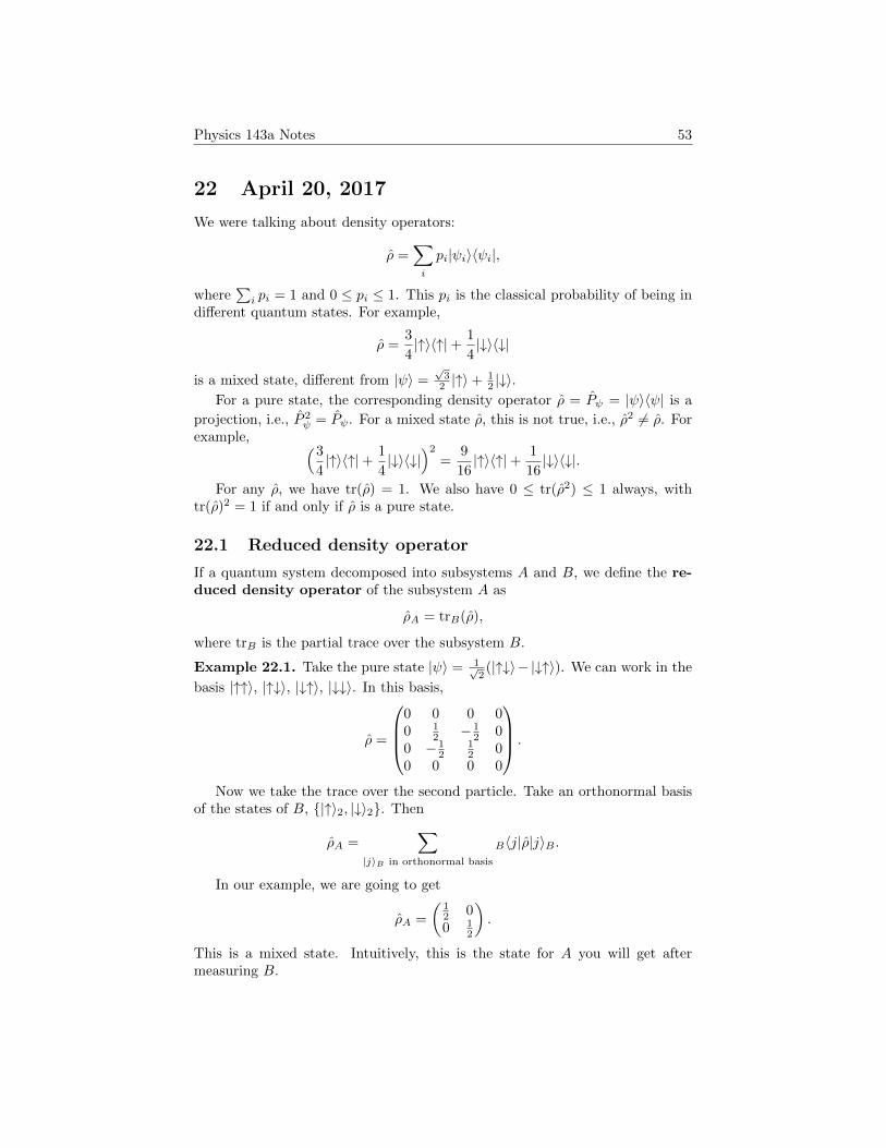
ρ =∑i
pi|ψi〉〈ψi|,
where∑i pi = 1 and 0 ≤ pi ≤ 1. This pi is the classical probability of being in
different quantum states. For example,
ρ =3
4|↑〉〈↑|+ 1
4|↓〉〈↓|
is a mixed state, different from |ψ〉 =√
32 |↑〉+ 1
2 |↓〉.For a pure state, the corresponding density operator ρ = Pψ = |ψ〉〈ψ| is a
projection, i.e., P 2ψ = Pψ. For a mixed state ρ, this is not true, i.e., ρ2 6= ρ. For
example, (3
4|↑〉〈↑|+ 1
4|↓〉〈↓|
)2
=9
16|↑〉〈↑|+ 1
16|↓〉〈↓|.
For any ρ, we have tr(ρ) = 1. We also have 0 ≤ tr(ρ2) ≤ 1 always, withtr(ρ)2 = 1 if and only if ρ is a pure state.
22.1 Reduced density operator
If a quantum system decomposed into subsystems A and B, we define the re-duced density operator of the subsystem A as
ρA = trB(ρ),
where trB is the partial trace over the subsystem B.
Example 22.1. Take the pure state |ψ〉 = 1√2(|↑↓〉− |↓↑〉). We can work in the
basis |↑↑〉, |↑↓〉, |↓↑〉, |↓↓〉. In this basis,
ρ =
0 0 0 00 1
2 − 12 0
0 − 12
12 0
0 0 0 0
.
Now we take the trace over the second particle. Take an orthonormal basisof the states of B, {|↑〉2, |↓〉2}. Then
ρA =∑
|j〉B in orthonormal basis
B〈j|ρ|j〉B .
In our example, we are going to get
ρA =
(12 00 1
2
).
This is a mixed state. Intuitively, this is the state for A you will get aftermeasuring B.
Physics 143a Notes 54
In this example,
ρ2A =
(1/4 00 1/4
)6= ρA
so the reduced density matrix is not a projection operator even though thecomplete 2-state is pure. This is the hallmark of entanglement. Subsystems Aand B and entangled if and only if ρA = trB ρ is not a projection operator.
22.2 Decoherence and interpretation of quantum physics
These are examples of open quantum systems. We have access to only a subsetof the degrees of freedom of the system. This is very important for the emergenceof classical physics from the microscopic law of quantum mechanics. There is atension in the laws of quantum mechanics:
(1) Given |ψ(0)〉 and H, you can tell me |ψ(t)〉 = e−iHt/~|ψ(0)〉.(2) If you measure a state, you change it to an eigenstate of what you measure,
with some probability.
You can consider the whole measuring device as a quantum state, but the firstlaw seems deterministic and the second law seems uncertain and random. Therehas been a lot of discussion on these among physicists and philosophers, andthere is a whole subject on interpretation of quantum physics.
This is related to the decoherence and measurement. Suppose I have a |+x〉particle and we feed it to a +z Stern–Gerlach device, with one light turning onif it goes up and another light turning on if it goes down. This whole apparatusis a very complex system:
1√2
(|+z〉+ |−z〉)⊗ |measuring device, lights off〉 ⊗ |air in the room〉 ⊗ · · · .
If our measuring device worked as we wanted, this is going to be[ 1√2
∣∣∣+z,upper lightsturned on
⟩+
1
2
∣∣∣−z, lower lightsturned on
⟩]⊗ |air in the room〉 ⊗ · · · .
If more time passes, you are going to get
1√2
∣∣∣+z,upper lightsturned on
,atoms in air
in state (# 1)
⟩+
1
2
∣∣∣−z, lower lightsturned on
,atoms in air
in state (# 2)
⟩.
So the measuring device correlate a microscopic quantum state with a hugenumber of other particles. You can never measure the entire air, and What youcan access is described by the reduced density density matrix tracing over theair’s state. This is effective like the classical probability.

Physics 143a Notes 55
22.3 Bell’s inequality
A lot of people tried to make different theories that agree with experimentalresults, but failed. Bell was one of those people, and in the course, he showedsomething that need to be true. Bell’s inequality is one of them, and I am goingto present one version from John Preskill’s lecture notes.
Two experimenters, Alice and Bob play a game. Each flip a coin, and theymay share some information beforehand. These information has to be classicalor an entangled quantum state
1√2
(|↑↑〉+ |↓↓〉).
They communicate a bit (classical 0 or 1) and the sefult of their coin flip. Theywin the game if “the XOR of the bits they send is 0 if and only if both coinsshow heads”.
Here is a classical strategy that winds 75% of the time. Both Alice say 0.Then they lose exactly when the coins are both heads.
It turns out this is the best possible strategy. This follows from the CHSH(Clauser–Horne–Shimony–Holt) inequality. For four number αH , αT , βH , βT ,each of which is ±1, we have
C = (αH + αT )βT + (αT − αH)βH = ±2
and so|〈αTβT 〉+ 〈αTβH〉+ 〈αHβT 〉 − 〈αHβH〉| ≤ 2.
Let αH = 1 if Alice says 0 if the when she sees H, and αH = −1 if Alicesays 1 when she sees T . Then if you work out,
|2(pTT + pTH + pHT + pHH)− 4| ≤ 2
and so the average winning probability is (1/4)∑pIj ≤ 3/4.
Physics 143a Notes 56
23 April 25, 2017
We were talking about Alice and Bob, who can share information in advance.They flip a coin, choose a bit and communicate the results. They win if bothcoins are heads and the XOR of their bits is true, or one of the coins are tailsand the XOR of their bits is false.
There is an easy classical 75% winning strategy: both say false always. Itturned out that this is the best possible due to the CHSH inequality, which issimilar to the Bell inequality. If αT is the random variable
αT =
{−1 if Alice says true when she sees tails,
1 if Alice says false when she sees tails,
and define other variables αH , βH , βT analogously, then the CHSH inequalitysays
|〈αTβT 〉+ 〈αTβH〉+ 〈αHβT 〉 − 〈αHβH〉| ≤ 2.
Now our claim is that 〈αTβT 〉 is 2pwinTT −1 where pwin
TT is the conditional prob-ability of winning when the coins are both tails. Similar interpretations work,and so the overall probability of winning is 1
4
∑i,j p
winij . Then the inequality
tells us ∣∣∣∣2∑i,j
pwinij − 4
∣∣∣∣ ≤ 1.
So the probability of wining for any strategy based on classical probability is atmost 75%.
23.1 A quantum mechanical strategy
Now suppose that Alice and Bob share an entangled pair of spins
〈ψ〉 =1√2
(|↑〉A ⊗ |↑|B − |↓〉A ⊗ |↓〉B).
Here is a strategy that wins more that 75% of the time.
• If Alice sees heads, she measures the spin’s z-component, and says true ifshe sees +~/2 and false if she sees −~/2.
• If Alice sees tails, she first act on her state with the unitary matrix
U =
(cos 3π/8 − sin 3π/8sin 3π/8 cos 3π/8
)and then measures the z-component of the spin, and says true if she sees+~/2 and false if she sees −~/2.
• Bob does the same thing, but gives the opposite answers: false if +~/2and true if −~/2.

Physics 143a Notes 57
Now let us calculate the probability of winning.
(1) Alice and Bob both see heads.
The winning condition is that they disagree. Then either they both sees↑ or both sees ↓. So they win 100% of the time.
(2) Alice sees heads, Bob sees tails.
It doesn’t matter, but let’s assume Alice first does the measurement. Then1/2 of the time she sees ↑ and says T , and 1/2 of the time she sees ↓ andsays F . If Alice sees ↑, this measurement effectively collapses Bob’s stateinto |↑〉B and after acting by U , it becomes
U
(10
)=
(cos 3π/8sin 3π/8
).
So Bob cos2 3π/8 of the time sees ↑ and says F , and sin2 3π/8 of the timesees ↓ and says T .
Alice sees ↓ for 1/2 of the time F , and says F . Likewise, Bob says Fwith probability sin2 3π/8 and T with probability cos2 3π/8. So they winsin2 3π/8 of the time in total.
(3) Alice sees tails, Bob sees heads.
This is going to be the same probability of sin2 3π/8 of winning, becauseit is basically case (2).
(4) Alice and Bob both see tails.
They win if they say the same thing. Suppose Alice goes first. The statebecomes
1√2
[cos
3π
8|↑↑〉+ sin
3π
8|↓↑〉+ sin
3π
8|↑↓〉 − cos
3π
8|↓↓〉
].
When Alice measures, 50% times of the time she sees |↑〉 and project Bobonto cos 3π/8|↑〉B + sin 3π/8|↓〉B . Now Bob sees tails so acting on U gives
U
(cos 3π/8sin 3π/8
)=
(cos 3π/4sin 3π/4
).
Then they in 50% of the time. Same goes for when Alice sees |↓〉. Sooverall they win 50% of the time.
So the overall chance of winning is
1
4
[1 + 2 sin2 3π
8+
1
2
]≈ 0.80 > 0.75.
The lesson of all this is that quantum entanglement is distinctly quantum phe-nomenon; no complicated classical theory can do the same thing.
Another lesson is that quantum entanglement can be a resource. This is thebasic premise behind quantum computing, quantum cryptography, . . . . If you’reinterested in these kinds of stuff, you can read Preskill’s lecture notes on quan-tum information, Nielson and Chuany’s Quantum Information and QuantumComputing.
Physics 143a Notes 58
23.2 No-cloning theorem and quantum transportation
This basically says that you can’t copy a quantum state. That is, there is nomap
U : |ψ〉 ⊗ |0〉 7→ |ψ〉 ⊗ |ψ〉.
This is because of linearity. If we assume U(|0〉 ⊗ |0〉) = |00〉 and U(|1〉 ⊗ |0〉) =|11〉, then for |ψ〉 = a|0〉+ b|1〉,
U(|ψ〉 ⊗ |0〉) = a|00〉+ b|11〉 6= (a|0〉+ b|1〉)⊗ (a|0〉+ b|1〉).
We can’t clone information, but could we transmit it?
|ψ〉 ⊗ |χ〉 7→ |ξ〉 ⊗ |ψ〉
We can do this if we share an entangled state, even without being at the sameplace.
Here is the idea. Let Alice have the qubit |ψ〉C = α|0〉C + β|1〉C . She wantsto send this to Bob. Suppose Alice and Bob share an entangled state
|Φ+〉 =1√2
(|00〉AB + |11〉AB).
The three particles state can be written as
|ψ〉C ⊗ |Φ+〉AB =1√2
(α|000〉CAB + α|011〉CAB + β|100〉CAB + β|111〉CAB)
=1
2|Φ+〉CA ⊗ (α|0〉B + β|1〉B) +
1
2|Φ−〉CA ⊗ (α|0〉B − β|1〉B)
+1
2|Ψ+〉CA ⊗ (α|1〉B + β|0〉B) +
1
2|Ψ−〉CA ⊗ (α|1〉 − β|0〉B),
where
|Φ±〉CA =1√2
(|00〉CA ± |11〉CA), |Ψ±〉CA =1√2
(|01〉CA ± |10〉CA).
Now Alice’s goal is to project onto one of |Φ±〉CA, |Ψ±〉CA. Note that shehas access to the particles C and A. If the outcome is |Φ+〉CA, then she knowsthat Bob’s state would be a copy. If the outcome is |Φ−〉CA, then Alice couldcall Bob and tell him to act with ( 1 0
0 −1 ). To project it, Alice can apply theCNOT operation.
You still need to send some classical information. So complete quantumtransportation is not possible faster than the speed of light.

Index
Bohr radius, 50
CHSH inequality, 55commutator, 12
density operator, 52reduced, 53
Dirac delta, 25Dirac notation, 5
energy-time uncertainty relation,22
entangled state, 51
Fourier transform, 27
Gaussian wave, 27
Hamiltonian, 20harmonic oscillator, 34hermitian, 10
ladder operators, 33Lie algbera, 15
mixed state, 52momentum operator, 25
number operator, 35
orbital angular momentum, 43
parity operator, 36plane wave, 26position operator, 25principal quantum number, 50probability current, 32projection operator, 11pure states, 52
qubit, 5
reflection coefficient, 32representation, 15Rydberg constant, 50
Schrodinger equation, 20spherical harmonics, 44spin-j representation, 17stationary state, 20
transmission coefficient, 32tunneling, 32
uncertainty, 13uncertainty principle, 13
Heisenberg’s, 26unitary matrix, 7
wave function, 24
59