Physica A 424 (2015) 34–43

Contents lists available at ScienceDirect

Physica A

journal homepage: www.elsevier.com/locate/physa

Some statistical equilibrium mechanics and stabilityproperties of a class of two-dimensional Hamiltonianmean-field modelsJ.M. Maciel a,b, M.-C. Firpo a,∗, M.A. Amato b

a Laboratoire de Physique des Plasmas, CNRS-Ecole Polytechnique, 91128 Palaiseau cedex, Franceb Instituto de Fisica, Universidade de Brasília, Brasília, DF, Brazil

h i g h l i g h t s

• Cold atoms may become a playground to prepare long-range systems in the laboratory.• In this purpose, a class of 2D long-range mean-field models is introduced.• The long-range interaction may be attractive, repulsive or a mixture of both cases.• Microcanonical Monte Carlo computations allow us to determine equilibrium.• A Bravais-like lattice is introduced to classify the low-energy real 2D-space structure.

a r t i c l e i n f o

Article history:Received 10 October 2014Received in revised form 16 December 2014Available online 5 January 2015

Keywords:Long-range interacting systemsMean-field modelsQuasi-stationary statesCold atomsMagnetic trapsLaser cooling

a b s t r a c t

A two-dimensional class of mean-field models that may serve as a minimal model to studythe properties of long-range systems in two space dimensions is considered. The statisticalequilibriummechanics is derived in themicrocanonical ensemble usingMonte Carlo simu-lations for different combinations of the coupling constants in the potential leading to fullyrepulsive, fully attractive andmixed attractive–repulsive potential along the Cartesian axisand diagonals. Then, having inmind potential realizations of long-range systems using coldatoms, the linear theory of this two-dimensionalmean-field Hamiltonianmodels is derivedin the low temperature limit.

© 2015 Elsevier B.V. All rights reserved.

1. Introduction

There is now a large amount of experimental and theoretical studies demonstrating that the classical picture of relax-ation driven by two-body collisions fails to correctly describe transport in long-range interacting systems [1]. Historically,the first striking identifications of the peculiar relaxation properties of long-range systems came from space observations. Inthe middle of the 1960s, it was found that the luminosity profiles of elliptical galaxies were regular, smooth and symmetric,which suggested that they had reached some equilibrium states. However, earlier calculations by Chandrasekhar [2] gaveestimations of the relaxation timescale due to two-body collisions much longer than the age of the universe contradictingan interpretation of the relaxation in terms of binary effects. This led Lynden-Bell to introduce the concept of ‘‘violent re-laxation’’ in his famous 1967 paper [3] as a collisionless scenario to account for the rapid evolution of the galaxies toward

∗ Corresponding author.E-mail address:marie-christine.firpo@lpp.polytechnique.fr (M.-C. Firpo).

http://dx.doi.org/10.1016/j.physa.2014.12.0300378-4371/© 2015 Elsevier B.V. All rights reserved.

brought to you by COREView metadata, citation and similar papers at core.ac.uk

provided by Elsevier - Publisher Connector

J.M. Maciel et al. / Physica A 424 (2015) 34–43 35

quasi-stationary or quasi-equilibrium states. Lynden-Bell’s proposal initiated a much debated and active field of researchthat progressively diffused from the space physics community to the statistical physics community. This was helped by theuse of simplified models of self-gravitating systems. In particular, much progress in the understanding of the relaxationproperties of systems interacting via long-ranges forces originated from numerical simulations of the one-dimensionalgravitational system. Various extensive numerical observations pointed to the following scenario: the relaxation of one-dimensional self-gravitatingN-body systems usually proceeds through a rapid approach to a quasi-stationary state (QSS) [4],in a sequence referred to as violent relaxation, followed by a very slow drift toward equilibrium [5,6]. A much investigatedissue has been the scalings with N of these different dynamical sequences, such as the lifetimes of QSSs [7]. Meanwhile, thecommunity of statistical physics began to study the intricate interplay between dynamics, ergodic properties and statisticalmechanics in long-range Hamiltonian systems through the use of even more simplified and reduced ‘‘toy’’ models, a well-known example being the so-called HamiltonianMean Field (HMF)model [8]. This model has proven to be a sort of minimaland paradigmatic model to study long-range effects [9]. It has been a key framework to investigate the conditions for theemergence of QSSs [10–14] and the much debated issue of their lifetimes [15–17].

The HMFmodel is however one-dimensional in space, which could be quite a stringent restriction for experimental real-izations. Indeed, a few years ago emerged the proposal to use Bose–Einstein condensates as a physical playground to preparelong-range systems in the laboratory. In particular, O’Dell et al. [18] offered a proof of principle that particular configura-tions of intense off-resonant laser beams could realize an attractive gravitation-like interatomic potential between atoms.Moreover, in the HMFmodel, studying diffusion implicitly means studying the diffusion in the action-angle space. In a two-dimensional model, one could study the diffusion in the real 2D space. This led Torcini and Antoni [19] to introduce in 1999a two-dimensional counterpart of the HMFmodel. This consisted in an N-body system interacting via a classical long-rangeinterparticle potential in a 2D Cartesian periodic space in which only the longest wavelength modes are retained.

In the present study, the class of N-body Hamiltonian models that will be considered reads H = K + V with

K =

Ni=1

p2i,x + p2i,y2

, (1)

V =12N

Ni,j=1

c1 + c2 + d − c1 cos

xi − xj

− c2 cos

yi − yj

− d cos

xi − xj

cos

yi − yj

. (2)

For each particle i, pi,x is the momentum conjugated to xi and pi,y is the momentum conjugated to yi. K is the kinetic energyand V is the potential energy. c1, c2 and d denote constants. Compared with the original model introduced by Antoni andTorcini [20,19] having c1 = c2 = d = 1, we shall not restrict here to the purely attractive, gravitational or ferromagnetic-like, case and allow the system to be fully attractive (if c1, c2, d > 0), fully repulsive (if c1, c2, d < 0) or mixed (in theremaining cases). The reference energy is chosen in such a way that the energy of the system vanishes when all the particleshave the same position (V = 0) and zero velocity (K = 0).

It is a simple task to realize that the above Hamiltonian models, coming from (1)–(2), are of a mean-field nature. Indeed,introducing the magnetization-like mean-fields

M1 =

1N

Ni=1

cos xi,1N

Ni=1

sin xi

≡ M1 (cosφ1, sinφ1) (3)

M2 =

1N

Ni=1

cos yi,1N

Ni=1

sin yi

≡ M2 (cosφ2, sinφ2) (4)

and the polarization-like mean-fields

P1 =

1N

Ni=1

cos (xi + yi) ,1N

Ni=1

sin (xi + yi)

≡ P1 (cosψ1, sinψ1) , (5)

P2 =

1N

Ni=1

cos (xi − yi) ,1N

Ni=1

sin (xi − yi)

≡ P2 (cosψ2, sinψ2) (6)

enables us to write the class of Hamiltonian systems H associated to (1)–(2) in the compact form

H =

Ni=1

p2i,x + p2i,y2

+12N

Ni,j=1

c1 + c2 + d − c1M2

1 − c2M22 −

d2(P2

1 + P22 )

, (7)

where the potential is a function of themoduli of the mean-fields only, and to obtain the corresponding one-particle Hamil-tonian systems h = H/N as

h =p2x2

+p2y2

+ c1 + c2 + d − c1M1 cos (x − φ1)− c2M2 cos (y − φ2)

− dP12

cos (x + y − ψ1)− dP22

cos (x − y − ψ2) . (8)

36 J.M. Maciel et al. / Physica A 424 (2015) 34–43

The objective of the present study is first to derive the equilibrium statistical mechanics of the above systems througha microcanonical Monte Carlo approach. This may be viewed as a prerequisite for future investigations of the relaxationproperties of the 2D mean-field models and will be presented in Section 2. Then, having in mind the potential applicationsof these models to cold atom systems, we shall turn to the derivation of the linear theory in the low temperature limit inSection 3. Some conclusions and perspectives are briefly drawn in Section 4.

2. Equilibrium statistical mechanics in the microcanonical ensemble

2.1. The microcanonical Monte Carlo method

Computer simulations using Monte Carlo methods are extensively used in theoretical physics [21–24]. In the originalform of the Monte Carlo method, one determines configurations using the Metropolis et al. algorithm, which generatesthe equilibrium configurations of the canonical ensemble [21,25,24]. In this respect, a useful presentation of the canonicalMetropolis Monte Carlo algorithm may be found in Ref. [26]. Pluchino et al. perform there some canonical Monte Carlosimulations of the one-dimensional HMF model and use them to probe the stability of QSSs. However systems with long-range interactions can present inequivalence between the microcanonical and the canonical ensembles [9]; hence it turnsout necessary to develop a Monte Carlo method which determines the equilibrium distribution of the microcanonicalensemble. The first attempt to develop a microcanonical algorithm was made by Creutz [27]. However his algorithm wasnot truly microcanonical since it introduces a demon which interacts with the system [24]. Then, Ray [21] developeda modified Metropolis algorithm that generates the microcanonical ensemble configurations. Ray’s differs from Creutz’salgorithm method in avoiding the random walk in the momenta space and also eliminating the demon trick. This puts theMicrocanonical Monte Carlo Algorithm (MMCA) on equal footing with the canonical Metropolis algorithm [21].

In the microcanonical ensemble, the phase space volume has the form

Ω(E, V ,N) = C(N)Θ[E − H(pi, qi)]

Ni=1

ddpiddqi (9)

whereΘ denotes the Heaviside step function, d is the dimension of the system and C(N) is a constant that depends only onN . If the Hamiltonian has the form H(pi, qi) =

Ni=1 pi

2/2m + V (qi) and one performs the integration over momentaspace, the phase space volume in Eq. (9) can be reduced to Ref. [21]

Ω(E, V ,N) = C ′(N)

[E − V (qi)]dN2 −1Θ[E − V (qi)]

Ni=1

ddqi, (10)

where C ′(N) is another constant, which depends only on N . By Eq. (10), the probability density is given by [21]

WE(qi) = C ′(N)[E − V (qi)]dN2 −1Θ[E − V (qi)], (11)

where the Heaviside step function avoids negative kinetic energies. In order to implement the microcanonical Monte Carlomethod, the acceptance probability of the Metropolis algorithm can be defined by Eq. (11) [21]

PE(qi → q′i) = min

1,

[K(q′

i)]dN2 −1Θ[K(q′

i)]

[K(qi)]dN2 −1

, (12)

where K(qi) = E − V (qi) is the kinetic energy of the system in the previous configuration and K(q′

i) = E − V (q′

i) isthe kinetic energy of the system in the new configuration. The entropy in the microcanonical ensemble is given by

S(E, V ,N) = kB lnΩ(E, V ,N). (13)

The usual thermodynamic properties can be obtained by differentiation of the entropy with respect to thermodynamicvariables [21]. In particular, the temperature is determined by the relation T−1

= ∂S/∂E yielding

T =

2

dNkB

⟨E − V (q)⟩ =

2

dNkB

⟨K(q)⟩ (14)

where the angular brackets imply averaging with respect to the probability density in Eq. (11).Practically, the MMCA has been implemented according to the following procedure:

1. Choose a particle nwith original position rn = r0n = (x0n, y0n).

2. Choose randomly a new position r′n = (x′n, y

′n) for the particle n.

3. Compute the kinetic energy of the system with particle n in the original configuration K(ri, rn = r0n) = K 0, using therelation K(ri) = E −

Nj,m=1 V (rj − rm).

4. Compute the kinetic energy of the system with particle n in the new configuration K(ri, rn = r′n) = K ′.5. If K 0

≤ K ′, the new configuration is accepted.

J.M. Maciel et al. / Physica A 424 (2015) 34–43 37

. .

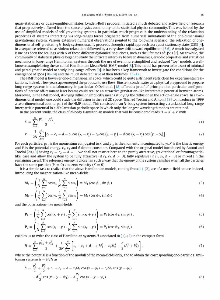
Fig. 1. Caloric curve and mean-field microcanonical ensemble averages for the fully attractive case obtained with N = 104 particles.

6. If K 0 > K ′, the new configuration is acceptedwith a probability P(r0n → r′n) given by Eq. (12): generate a randomnumberR and compare it to the probability, if R ≤ P(r0n → r′n), then the new configuration is accepted, if R > P(r0n → r′n), thenew configuration is rejected.

7. Redo steps 1–6 until the kinetic energy of the system reaches a stable value.8. Compute the temperature using Eq. (14).

2.2. Numerical results

In order to obtain the microcanonical thermodynamical curves, the MMCA has been implemented with N = 104 par-ticles. From our numerical simulations it turns out that, for N roughly above 100, the caloric and the mean fields curvesbecome roughly independent of the number of particles N apart from phase transition regions where finite-N effects maybe detected. The averages were taken from 106 to 2.106 MMC iterations, a range within which the convergence toward theequilibrium distribution was checked to be effective with the help of a kurtosis inspection. Due to the isotropy of choicesin c1 = c2 and d, the mean fields M1 ≈ M2 and P1 ≈ P2 as N increases. In the remaining of the article, the numericalapplications will restrict for the sake of simplicity to the cases c1 = c2 = ±1 and d = ±1.

In Fig. 1, the energy dependence of the temperature and of themean-fields for the totally attractive, gravitation-like, caseare reportedwith c1 = c2 = d = 1. These results are in good agreementwith previous results obtained in the fully attractivemodel [19,28,29]. The system presents two phases: a highly inhomogeneous single-cluster cold phase (SCP) for energieslower than a critical energy (0 ≤ ε ≤ UA

C ≈ 2), that exhibits a negative specific heat region in the range 1.25 ≤ ε ≤ UAC ,

and a homogeneous phase (HP) for values of energy higher than UC . The phase transition connecting the SCP with the HPphase is second order since the mean-field goes to zero continuously and the specific heat goes from a negative value to apositive value discontinuously. The SCP distribution is displayed in Fig. 2.

The completely repulsive case is reported in Fig. 3. This case is less interesting in terms of its equilibrium properties.The homogeneous state is thermodynamically stable at all energies, the specific heat is always positive and constant and nophase transition is present.

The results for the mixed attractive–repulsive case are reported in Fig. 4. The mean fields M1 and M2 were chosen to bethe repulsive mean-fields, while the P1 and P2 to be the attractive mean-fields. Due to the Hamiltonian invariance underrotation by multiples of π/4, swapping theM and P mean-fields, namely by choosingM1 andM2 as attractive and P1 and P2as repulsive mean fields, would yield similar results.

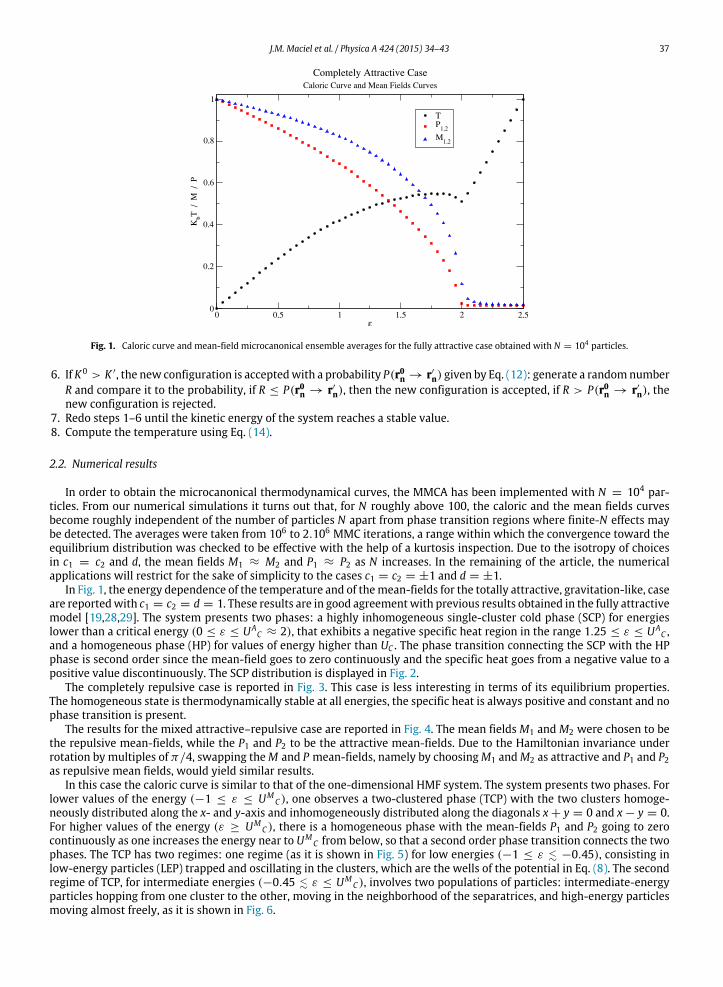
In this case the caloric curve is similar to that of the one-dimensional HMF system. The system presents two phases. Forlower values of the energy (−1 ≤ ε ≤ UM

C ), one observes a two-clustered phase (TCP) with the two clusters homoge-neously distributed along the x- and y-axis and inhomogeneously distributed along the diagonals x + y = 0 and x − y = 0.For higher values of the energy (ε ≥ UM

C ), there is a homogeneous phase with the mean-fields P1 and P2 going to zerocontinuously as one increases the energy near to UM

C from below, so that a second order phase transition connects the twophases. The TCP has two regimes: one regime (as it is shown in Fig. 5) for low energies (−1 ≤ ε . −0.45), consisting inlow-energy particles (LEP) trapped and oscillating in the clusters, which are the wells of the potential in Eq. (8). The secondregime of TCP, for intermediate energies (−0.45 . ε ≤ UM

C ), involves two populations of particles: intermediate-energyparticles hopping from one cluster to the other, moving in the neighborhood of the separatrices, and high-energy particlesmoving almost freely, as it is shown in Fig. 6.

38 J.M. Maciel et al. / Physica A 424 (2015) 34–43

Fig. 2. SCP real space distribution for ε = 0.3 in the fully attractive case. The particles are trapped in the single cluster structure.

Fig. 3. Caloric and mean-field curves for the fully repulsive case.

2.3. Low-energy real 2D-space structure: Bravais-like lattice

Due to the periodicity of the potential, one can increase the space period length by a multiple of 2π . So doing the systemforms a periodic structure which can be regarded as a two dimensional oblique Bravais-like lattice with a set of primitivevectors a1 = (π, π), and a2 = (2π, 0), shown in Fig. 7. This yields a1 =

√2π, a2 = 2π and φ = π/4, where ai are the

moduli of the primitive vectors andφ the angle between them. In solid state physics, the Bravais lattice specifies the periodicarray in which the repeated units of a crystal (in the present case group of particles) are arranged [30]. In this way the TCPphase can be seen as a solid phase.

3. Linear theory in the cold limit

In this section, the linear stability of the cold 2D HMF systems will be considered.

3.1. Kinetic limit

From the equation of the one-particle Hamiltonian (8), one derives the equations of motionsdxdt

= px,

J.M. Maciel et al. / Physica A 424 (2015) 34–43 39

Fig. 4. Caloric curve and the mean-field curves for the mixed attractive–repulsive case. For low energies, the system is in the TCP, with two clustershomogeneously distributed along the axes x and y, but inhomogeneously distributed along the diagonals x + y = 0 and x − y = 0, yielding to zeromagnetizationsM1 andM2 , but non-zero polarizations P1 and P2 .

Fig. 5. Real space distribution for the low-energy regime for the TCP in the mixed attractive–repulsive case. LEP trapped in clusters.

dydt

= py,

dpxdt

= −

c1M1 sin (x − φ1)+ d

P12

sin (x + y − ψ1)+ dP22

sin (x − y − ψ2)

,

dpydt

= −

c2M2 sin (y − φ2)+ d

P12

sin (x + y − ψ1)− dP22

sin (x − y − ψ2)

.

The class of 2D Hamiltonian models being of mean-field nature, the corresponding Vlasov equation for the particles can bestraightforwardly written as

∂ f∂t

+ px∂ f∂x

+ py∂ f∂y

−

c1M1 sin (x − φ1)+ d

P12

sin (x + y − ψ1)+ dP22

sin (x − y − ψ2)

∂ f∂px

−

c2M2 sin (y − φ2)+ d

P12

sin (x + y − ψ1)− dP22

sin (x − y − ψ2)

∂ f∂py

= 0. (15)

40 J.M. Maciel et al. / Physica A 424 (2015) 34–43

Fig. 6. Real space distribution for the intermediate-energy regime (ε = −0.1) in the mixed attractive–repulsive case. In addition to LEP, this regimepresents two other populations of particles: intermediate-energy particles hopping from cluster to cluster and high-energy particles moving almost freely.

Fig. 7. Bravais-like lattice generated by a set of discrete translation operations described by R = n1a1 + n2a2 corresponding to the low-energy regime(ε ≈ −1) two-clustered phase in the mixed attractive–repulsive case.

In this work, we shall derive the linear stability of the 2D Hamiltonianmean-field models only in the low temperature limit.This enables us to simplify the linear analysis by using a cold fluid assumption. Therefore this amounts to replace the linearstudy of the Vlasov kinetic equation (15) with that of a system of fluid equations. Let us introduce the moments of thedistribution function

n(r, t) = n(x, y, t) =

f (x, y, px, py, t) dpx dpy,

vx(r, t) =1

n(r, t)

pxf (x, y, px, py, t) dpx dpy,

vy(r, t) =1

n(r, t)

pyf (x, y, px, py, t) dpx dpy.

Let us then consider the moment equations of Eq. (15). The equation accounting for mass conservation reads

∂n∂t

+∂

∂x(n(r, t)vx(r, t))+

∂

∂y

n(r, t)vy(r, t)

= 0. (16)

Under the other cold fluid approximation, the distribution function may be written as

f (x, y, px, py, t) = n(r, t)δ (px − vx(r, t)) δpy − vy(r, t)

. (17)

J.M. Maciel et al. / Physica A 424 (2015) 34–43 41

Using this expression (17) in the first moment equations, with respect to px and py, of the Vlasov equation (15), we obtainfor the moment equation with respect to px

∂

∂t(nvx)+

∂

∂x

nv2x

+∂

∂y

nvxvy

+

c1M1 sin (x − φ1)+ d

P12

sin (x + y − ψ1)+ dP22

sin (x − y − ψ2)

n = 0, (18)

and some analogous equation for the moment equation with respect to py. The expressions of the mean-field vectors are

M1 =

cos(x)n(r, t) dx dy,

sin(x)n(r, t) dx dy

,

M2 =

cos(y)n(r, t) dx dy,

sin(y)n(r, t) dx dy

,

P1 =

cos(x + y)n(r, t) dx dy,

sin(x + y)n(r, t) dx dy

,

P2 =

cos(x − y)n(r, t) dx dy,

sin(x − y)n(r, t) dx dy

.

It is practical to use the Fourier decomposition along x and y, so that

n(r, t) =

∞m,l=−∞

nm,l(t) ei(mx+ly),

and introduce the complex expression of the mean-fields

M1 =

exp(ix)n(r, t) dx dy = (2π)2 n−1,0(t),

M2 =

exp(iy)n(r, t) dx dy = (2π)2 n0,−1(t),

P1 =

exp(ix) exp(iy)n(r, t) dx dy = (2π)2 n−1,−1(t),

P2 =

exp(ix) exp(−iy)n(r, t) dx dy = (2π)2 n−1,1(t).

3.2. Linear results

Linearizing the fluid equations about a homogeneous state with density n0 yields the linear system of equations for theperturbed density and velocity components

∂δn∂t

+ n0∂

∂x(δvx(r, t))+ n0

∂

∂y

δvy(r, t)

= 0,

∂

∂t(δvx)+ c1M1 sin (x − φ1)+ d

P12

sin (x + y − ψ1)+ dP22

sin (x − y − ψ2) = 0,

∂

∂t

δvy+ c2M2 sin (y − φ2)+ d

P12

sin (x + y − ψ1)− dP22

sin (x − y − ψ2) = 0.

Using a space and time Fourier decomposition

δn(r, t) =

kδnk ei(k.r−ωt) =

∞m,l=−∞

δnm,l ei(mx+ly−ωt),

δvx,y(r, t) =

kδv

x,yk ei(k.r−ωt) =

∞m,l=−∞

δvx,ym,l e

i(mx+ly−ωt),

where δn∗

m,l = δn−m,−l and δvx,y∗m,l = δv

x,y−m,−l yields

−ωδnm,l + mn0δvxm,l + ln0δv

ym,l = 0,

∞m,l=−∞

−iωδvxm,l ei(mx+ly)

+ (2π)2 Imc1 eixδn1,0 + d eix+iy δn1,1

2+ d eix−iy δn1,−1

2

= 0,

∞m,l=−∞

−iωδvym,l ei(mx+ly)

+ (2π)2 Imc2 eiyδn0,1 + d eix+iy δn1,1

2− d eix−iy δn1,−1

2

= 0.

42 J.M. Maciel et al. / Physica A 424 (2015) 34–43

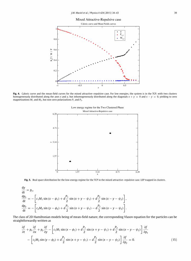
Fig. 8. Molecular dynamics simulations for the cold 2D HMFmodel in the mixed case with N = 100,000 particles. As can be seen from the inset, the lineargrowth rate is about 1/

√2 which in agreement with the theoretical predictions.

After some straightforward calculations, the relation dispersion may be expressed as the diagonal system of equationsω +

d2ω

δn1,1 = 0,

ω +c12ω

δn1,0 = 0,

ω +d2ω

δn1,−1 = 0,

ω +c22ω

δn0,1 = 0,

ωδn0,0 = 0.

Therefore, the stability of the system is conditioned by the signs of the interaction potential since the non-zero complexeigenfrequencies are the solutions of

ω2= −

d2, (19)

ω2= −

c12, (20)

ω2= −

c22. (21)

From (19)–(21), it follows that only the fully repulsive models are linearly stable in the cold fluid limit.Fig. 8 shows the early stage of the time evolution of the mean-field P1 for the cold 2D Hamiltonian model with a mixed

attractive/repulsive long-range potential. This curve has been obtained using a fourth-order symplectic code to integratethe 2D HMF particle dynamics (the complete description of the algorithm can be obtained in the Refs. [31,32]). In the caseof Fig. 8, the system is composed of a large number (105) of particles allowing to reproduce quite well the kinetic N → ∞

behavior, at least during early times. The initial growth is exponential and the linear growth rate γL is in agreement withthe theoretical prediction γL = Im(ω) = 1/

√2.

4. Conclusion

In this study, the equilibrium statistical mechanics of some 2D Hamiltonian mean-field models has been derived in themicrocanonical ensemble. The already documented attractive, gravitation-like, case has served as a testbed for the micro-canonical Monte Carlo code. The main novelty lies in the derivation of the mixed attractive–repulsive situation. Along therepulsive direction, the system behaves as the 1D antiferromagnetic HMF model, whereas along the attractive direction, itbehaves as the 1D gravitational or ferromagnetic HMFmodel, except that the low-energy condensed phase exhibits a biclus-ter instead of a single cluster phase. Then the linear theory for the cold 2D long-rangemodels has been derived. Furtherworkwill be devoted to the transport properties of the mixed repulsive/attractive 2D HMF models in the low temperature limit.

J.M. Maciel et al. / Physica A 424 (2015) 34–43 43

Acknowledgments

JMM thanks the Coordenação de Aperfeiçoamento de Pessoal de Nível Superior (CAPES) for financing his stay atEcole Polytechnique through the Programa Institucional de Bolsas de Doutorado Sanduíche no Exterior (PDSE) with grant7716-13-3. MAA acknowledges CNPq for financial support with grant CNPq 305825/2012. Fruitful discussions withX. Leoncini, D. Comparat, L. Pruvost and C. Josserand are gratefully acknowledged.

References

[1] D. Benest, C. Froeschle, E. Lega (Eds.), Topics in Gravitational Dynamics, in: Lecture Notes in Physics, vol. 729, 2007.

[2] S. Chandrasekhar, Principles of Stellar Dynamics, in: Astrophysical Monographs, Dover Publications, 1942, URL http://books.google.fr/books?id=UC52AAAAIAAJ.

[3] D. Lynden-Bell, Statistical mechanics of violent relaxation in stellar systems, Mon. Not. R. Astron. Soc. 136 (1967) 101. URL http://adsabs.harvard.edu/abs/1967MNRAS.136..101L.

[4] H. Wright, B. Miller, W. Stein, The relaxation time of a one-dimensional self-gravitating system, Astrophys. Space Sci. 84 (2) (1982) 421–429.http://dx.doi.org/10.1007/BF00651321.

[5] C.J. Reidl, B.N. Miller, Population dependence of early relaxation, Phys. Rev. E 51 (1995) 884–888. http://dx.doi.org/10.1103/PhysRevE.51.884. URLhttp://link.aps.org/doi/10.1103/PhysRevE.51.884.

[6] W. Ettoumi, M.-C. Firpo, Linear theory and violent relaxation in long-range systems: a test case, J. Phys. A 44 (17) (2011) 175002. URL http://stacks.iop.org/1751-8121/44/i=17/a=175002.

[7] T. Tsuchiya, N. Gouda, T. Konishi, Relaxation processes in one-dimensional self-gravitating many-body systems, Phys. Rev. E 53 (1996) 2210–2216.http://dx.doi.org/10.1103/PhysRevE.53.2210. URL http://link.aps.org/doi/10.1103/PhysRevE.53.2210.

[8] M. Antoni, S. Ruffo, Clustering and relaxation in hamiltonian long-range dynamics, Phys. Rev. E 52 (1995) 2361–2374. http://dx.doi.org/10.1103/PhysRevE.52.2361. URL http://link.aps.org/doi/10.1103/PhysRevE.52.2361.

[9] A. Campa, T. Dauxois, S. Ruffo, Statistical mechanics and dynamics of solvable models with long-range interactions, Phys. Rep. 480 (3–6) (2009)57–159. http://dx.doi.org/10.1016/j.physrep.2009.07.001. URL http://www.sciencedirect.com/science/article/pii/S0370157309001586.

[10] P.-H. Chavanis, Quasi-stationary states and incomplete violent relaxation in systems with long-range interactions, in: Fundamental Problems ofModern Statistical Mechanics Proceedings of the 3rd International Conference on ‘News, Expectations and Trends in Statistical Physics’, Physica A 365(1) (2006) 102–107. http://dx.doi.org/10.1016/j.physa.2006.01.006. URL http://www.sciencedirect.com/science/article/pii/S0378437106000458.

[11] A. Pluchino, A. Rapisarda, C. Tsallis, A closer look at the indications of q-generalized central limit theorem behavior in quasi-stationary states ofthe HMF model, Physica A 387 (13) (2008) 3121–3128. http://dx.doi.org/10.1016/j.physa.2008.01.112. URL http://www.sciencedirect.com/science/article/pii/S0378437108001222.

[12] X. Leoncini, T.L.V.D. Berg, D. Fanelli, Out-of-equilibrium solutions in the XY-Hamiltonian Mean-Field model, Europhys. Lett. 86 (2) (2009) 20002. URLhttp://stacks.iop.org/0295-5075/86/i=2/a=20002.

[13] M.-C. Firpo, Unveiling the nature of out-of-equilibriumphase transitions in a systemwith long-range interactions, Europhys. Lett. 88 (3) (2009) 30010.URL http://www.sciencedirect.com/science/article/pii/S0375960105007747.

[14] A. Turchi, D. Fanelli, X. Leoncini, Existence of quasi-stationary states at the long range threshold, in: sI:Complex Systems and Chaos with Fractionality,Discontinuity, and Nonlinearity, Commun. Nonlinear Sci. Numer. Simul. 16 (12) (2011) 4718–4724. http://dx.doi.org/10.1016/j.cnsns.2011.03.013.URL http://www.sciencedirect.com/science/article/pii/S1007570411001432.

[15] Y.Y. Yamaguchi, J. Barré, F. Bouchet, T. Dauxois, S. Ruffo, Stability criteria of the Vlasov equation and quasi-stationary states of theHMFmodel, Physica A337 (1–2) (2004) 36–66. http://dx.doi.org/10.1016/j.physa.2004.01.041. URL http://www.sciencedirect.com/science/article/pii/S0378437104001256.

[16] W. Ettoumi, M.-C. Firpo, Stochastic treatment of finite-N effects inmean-field systems and its application to the lifetimes of coherent structures, Phys.Rev. E 84 (3) (2011) 030103. URL http://link.aps.org/doi/10.1103/PhysRevE.84.030103.

[17] W. Ettoumi, M.-C. Firpo, Action diffusion and lifetimes of quasistationary states in the Hamiltonian mean-field model, Phys. Rev. E 87 (2013) 030102.http://dx.doi.org/10.1103/PhysRevE.87.030102. URL http://link.aps.org/doi/10.1103/PhysRevE.87.030102.

[18] D. O’Dell, S. Giovanazzi, G. Kurizki, V.M. Akulin, Bose–Einstein condensateswith 1/r interatomic attraction: electromagnetically induced gravity, Phys.Rev. Lett. 84 (25) (2000) 5687–5690. http://dx.doi.org/10.1103/PhysRevLett.84.5687.

[19] A. Torcini, M. Antoni, Equilibrium and dynamical properties of two-dimensional n-body systems with long-range attractive interactions, Phys. Rev. E59 (1999) 2746–2763. http://dx.doi.org/10.1103/PhysRevE.59.2746. URL http://link.aps.org/doi/10.1103/PhysRevE.59.2746.

[20] M. Antoni, A. Torcini, Anomalous diffusion as a signature of a collapsing phase in two-dimensional self-gravitating systems, Phys. Rev. E 57 (1998)R6233–R6236. http://dx.doi.org/10.1103/PhysRevE.57.R6233. URL http://link.aps.org/doi/10.1103/PhysRevE.57.R6233.

[21] J.R. Ray, Microcanonical ensemble Monte Carlo method, Phys. Rev. A 44 (1991) 4061–4064. http://dx.doi.org/10.1103/PhysRevA.44.4061. URL http://link.aps.org/doi/10.1103/PhysRevA.44.4061.

[22] P. Allen, D. Tildesley, Computer Simulation of Liquids, Oxford Science Publications, Clarendon Press, 1987, URL http://books.google.fr/books?id=ibURAQAAIAAJ.

[23] M.H. Kalos, P.A. Whitlock, Monte Carlo Methods. Vol. 1: Basics, Wiley-Interscience, New York, NY, USA, 1986.[24] D. Landau, K. Binder, A Guide to Monte Carlo Simulations in Statistical Physics, Cambridge University Press, New York, NY, USA, 2005.[25] N. Metropolis, A.W. Rosenbluth, M.N. Rosenbluth, A.H. Teller, E. Teller, Equation of state calculations by fast computing machines, J. Chem. Phys. 21

(6) (1953) 1087–1092. http://dx.doi.org/10.1063/1.1699114. URL http://scitation.aip.org/content/aip/journal/jcp/21/6/10.1063/1.1699114.[26] A. Pluchino, G. Andronico, A. Rapisarda, A monte carlo investigation of the hamiltonian mean field model, Physica A 349 (1–2) (2005) 143–154.

http://dx.doi.org/10.1016/j.physa.2004.10.009. URL http://www.sciencedirect.com/science/article/pii/S0378437104013202.[27] M. Creutz, Microcanonical Monte Carlo simulation, Phys. Rev. Lett. 50 (1983) 1411–1414. http://dx.doi.org/10.1103/PhysRevLett.50.1411. URL

http://link.aps.org/doi/10.1103/PhysRevLett.50.1411.[28] M. Antoni, S. Ruffo, A. Torcini, First- and second-order clustering transitions for a systemwith infinite-range attractive interaction, Phys. Rev. E 66 (2)

(2002) 025103.[29] T.M.R. Filho, M.A. Amato, A. Figueiredo, A novel approach to the determination of equilibrium properties of classical hamiltonian systems with long-

range interactions, J. Phys. A 42 (16) (2009) 165001. URL http://stacks.iop.org/1751-8121/42/i=16/a=165001.[30] N. Ashcroft, N. Mermin, Solid State Physics, Saunders College, Philadelphia, 1976.[31] H. Yoshida, Construction of higher order symplectic integrators, Phys. Lett. A 150 (57) (1990) 262–268. http://dx.doi.org/10.1016/0375-

9601(90)90092-3. URL http://www.sciencedirect.com/science/article/pii/0375960190900923.[32] T.M.R. Filho, Molecular dynamics for long-range interacting systems on graphic processing units, Comput. Phys. Comm. 185 (5) (2014) 1364–1369.

http://dx.doi.org/10.1016/j.cpc.2014.01.008. URL http://www.sciencedirect.com/science/article/pii/S0010465514000216.