Physica A 445 (2016) 343–356

Contents lists available at ScienceDirect

Physica A

journal homepage: www.elsevier.com/locate/physa

Degree distribution and assortativity in line graphs ofcomplex networksXiangrong Wang a,∗, Stojan Trajanovski a, Robert E. Kooij a,b,Piet Van Mieghem a

a Faculty of Electrical Engineering, Mathematics and Computer Science, Delft University of Technology, Delft, The Netherlandsb TNO (Netherlands Organization for Applied Scientific Research), Delft, The Netherlands

h i g h l i g h t s

• We investigate the degree distribution and the assortativity of a line graph.• Degree distributions of line graphs and their original graphs are the same class.• Line graphs are assortative in most cases.• Assortativity of line graphs is not linearly related to the one of original graphs.• We find trees and non-trees with negative assortativity in their line graphs.

a r t i c l e i n f o

Article history:Received 17 July 2015Received in revised form 29 October 2015Available online 14 November 2015

Keywords:Degree distributionAssortativityLine graphComplex network

a b s t r a c t

Topological characteristics of links of complex networks influence the dynamical processesexecuted on networks triggered by links, such as cascading failures triggered by links inpower grids and epidemic spread due to link infection. The line graph transforms linksin the original graph into nodes. In this paper, we investigate how graph metrics in theoriginal graph are mapped into those for its line graph. In particular, we study the degreedistribution and the assortativity of a graph and its line graph. Specifically, we show, bothanalytically and numerically, the degree distribution of the line graph of an Erdős–Rényigraph follows the same distribution as its original graph. We derive a formula for theassortativity of line graphs and indicate that the assortativity of a line graph is not linearlyrelated to its original graph. Additionally, line graphs of various graphs, e.g. Erdős–Rényigraphs, scale-free graphs, show positive assortativity. In contrast, we find certain types oftrees and non-trees whose line graphs have negative assortativity.

© 2015 Elsevier B.V. All rights reserved.

1. Introduction

Infrastructures, such as the Internet, electric power grids and transportation networks, are crucial to modern societies.Most researches focus on the robustness of such networks to node failures [1,2]. Specifically, the effect of node failureson the robustness of networks is studied by percolation theory both in single networks [2] and interdependent networksthat interact with each other [3]. However, links frequently fail in various real-world networks, such as the failures oftransmission lines in electrical power networks, path congestions in transportation networks. The concept of a line graph,

∗ Corresponding author.E-mail address: x.wang-2@tudelft.nl (X. Wang).

http://dx.doi.org/10.1016/j.physa.2015.10.1090378-4371/© 2015 Elsevier B.V. All rights reserved.

344 X. Wang et al. / Physica A 445 (2016) 343–356

that transforms links of the original graph into nodes in the line graph, can be used to understand the influence of linkfailures on infrastructure networks.

An undirected graph with N nodes and L links can be denoted as G(N, L). The line graph l(G) of a graph G is a graph inwhich every node in l(G) corresponds to a link in G and two nodes in l(G) are adjacent if and only if the corresponding linksin G have a node in common [4]. The graph G is called the original graph of l(G).

Line graphs are applied in various complex networks. Krawczyk et al. [5] propose the line graph as a model of socialnetworks that are constructed on groups such as families, communities and school classes. Line graphs can also representprotein interaction networks where each node represents an interaction between two proteins and each link representspairs of interaction connected by a common protein [6]. By the line graph transformation, methodologies for nodes can beextended to solve problems related to links in a graph. For instance, the link chromatic number of a graph can be computedfrom the node chromatic number of its line graph [7]. An Eulerian path (that can be computed rather easily in polynomialtime) in a graph transforms to a Hamiltonian path (which is difficult to compute, in fact, the problem is NP-hard) in the linegraph. Evan et al. [8] use algorithms that produce a node partition in the line graph to achieve a link partition in order touncover overlapping communities of a network. Wierman et al. [9] improve the bond (link) percolation threshold of a graphby investigating site (node) percolation in its line graph.

Previous studies focus on various mathematical properties of line graphs. Whitney’s Theorem [10] states that, if linegraphs of two connected graphs G1 and G2 are isomorphic, the graphs G1 and G2 are isomorphic unless one is the completegraph K3 and the other one is the star K1,3. Krausz [11], Van Rooij andWilf [12] have investigated the conditions for a graphto be a line graph. Van Rooij andWilf [12] have studied the properties of graphs obtained by iterative usage of the line graphtransformation, e.g., the line graph l(G) of a graphG, the line graph l(l(G)) of the line graph l(G), etc. Furthermore, Harary [13]has shown that for connected graphs that are not path graphs, all sufficiently high numbers of iterations of the line graphtransformation produceHamiltonian graphs.1 The generation of a random line graph is studied in Ref. [14]. An original graphcan be reconstructed [15–17] from its line graph with a computational complexity that is linear in the number of nodes N .

In this paper, we analytically study the degree distribution and the assortativity of line graphs and the relation to thedegree distribution and the assortativity of their original networks. We show that the degree distribution in the line graphof the Erdős–Rényi graph follows the same pattern as the degree distribution in Erdős–Rényi. However, the line graph ofan Erdős–Rényi graph is not an Erdős–Rényi graph. Additionally, we investigate the assortativity of line graphs and showthat the assortativity is not linearly related to the assortativity in the original graphs. The line graphs are assortative in mostcases, yet line graphs are not always assortative. We investigate graphs with negative assortativity in their line graphs. Theremainder of this paper is organized as follows. The degree distribution of line graphs is presented in Section 2. Section 3provides the assortativity of line graphs. We conclude in Section 4.

2. Degree distribution

Random graphs are developed as models of real-world networks of several applications, such as peer-to-peer networks,the Internet and the World Wide Web. The degree distribution of Erdős–Rényi random graphs and scale free graphs arerecognized by the binomial distribution and the power law distribution, respectively. This section studies the degreedistribution of the line graphs of Erdős–Rényi and scale free graphs.

Let G(N, L) be an undirected graph with N nodes and L links. The adjacency matrix A of a graph G is an N × N symmetricmatrix with elements aij that are either 1 or 0 depending on whether there is a link between nodes i and j or not. The degreedi of a node i is defined as di =

Nk=1 aik. The degree vector d = (d1 d2 · · · dN) has a vector presentation as Au = d, where

u = (1, 1, . . . , 1) is the all-one vector. The adjacency matrix [4] of the line graph l(G) is Al(G) = RTR − 2I , where R is anN × L unsigned incidence matrix with Ril = Rjl = 1 if there is a link l between nodes i and j, elsewhere 0 and I is the identitymatrix. The degree vector dl(G) of the line graph l(G) is dl(G) = Al(G)uL×1. For an arbitrary node l in the line graph l(G), whichcorresponds to a link l connecting nodes i and j in graph G (as shown in Fig. 1), the degree dl of the node l follows

dl = di + dj − 2. (1)

The random variable Di denotes the degree of a randomly chosen node i in Erdős–Rényi graphs Gp(N) and (1) shows thatthe degree Dl of a link lwith end node i in the corresponding line graph is Dl = Di + Dj − 2.

Theorem 1. The degree distribution of the line graph l(Gp(N)) of an Erdős–Rényi graph Gp(N) follows a binomial distribution

Pr[Dl = k] =

2N − 4

k

pk(1 − p)(2N−4−k) (2)

with average degree E[Dl(Gp(N))] = (2N − 4)p.

1 A Hamiltonian graph is a graph possessing a Hamiltonian cycle which is a closed path through a graph that visits each node exactly once.

X. Wang et al. / Physica A 445 (2016) 343–356 345

Fig. 1. Node l in line graph l(G) corresponds to the link l in G.

Proof. Applying (1), the degree distribution Dl of a node l in a line graph is

Pr[Dl = k] = Pr[Di + Dj − 2 = k].

Using the law of total probability [18] yields

Pr[Dl = k] =

km=1

Pr[Dj = k − m + 2|Di = m]Pr[Di = m].

Since the random variables Di and Dj in Gp(N) are independent, we have

Pr[Dl = k] =

km=1

Pr[Dj = k − m + 2]Pr[Di = m]. (3)

An arbitrarily chosen (i.e. uniformly at random) node l in the line graph l(G) corresponds to an arbitrarily chosen link inG. The degree distribution [18] of the end node i of an arbitrarily chosen link in G is

Pr[Di = m] =mPr[D = m]

E[D](4)

where Pr[D = m] is the degree distribution of an arbitrarily chosen node in graph G and E[D] is the average degree of anarbitrarily chosen node. In an Erdős–Rényi graph, we have Pr[D = m] =

N−1m

pm(1 − p)N−1−m and E[D] = (N − 1)p. By

substituting (4) into (3) and applying the binomial distribution of random variables Di and Dj, we have

Pr[Dl = k] =

km=1

(k − m + 2)Pr[D = k − m + 2]E[D]

mPr[D = m]

E[D]

=

km=1

(k − m + 2) N−1k−m−2

pk−m+2(1 − p)N−1−(k−m+2)

(N − 1)pmN−1

m

pm(1 − p)N−1−m

(N − 1)p

= pk(1 − p)2N−4−kk

m=0

N − 2k − m

N − 2m

.

Using Vandermonde’s identitym+n

r

=r

k=0

mk

nr−k

, we arrive at (2). �

Theorem 1 illustrates that the degree distribution of the line graph l(G) of an Erdős–Rényi graph G follows a binomialdistribution with average degree E[Dl(G)] = (2N − 4)p. Compared to the average degree E[D] = (N − 1)p, the averagedegree of the line graph of the Erdős–Rényi graph is two times the average degree E[D] of the Erdős–Rényi graph minus 2p.

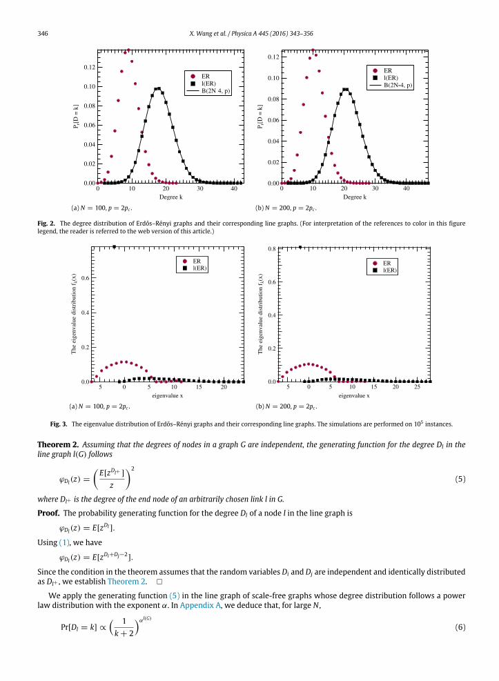
Fig. 2 shows the degree distribution of the line graphs of Erdős–Rényi graphs GN(p) for N = 100, 200 and p = 2pc(pc ≈

lnNN ), where 105 Erdős–Rényi graphs are generated. In Fig. 2(a) and (b), the degree distributions of Erdős–Rényi graphs

(red circle) follow a binomial distribution. The degree distribution of the corresponding line graph (black square) is fitted bya binomial distribution B(2N − 4, p). The simulation results agree with Theorem 1. Moreover, the average degree E[Dl(G)] ofthe line graph is approximately two times the average degree E[D] of the graph G.

Since the degree distribution of the line graphs of Erdős–Rényi graphs follows a binomial distribution, we pose thequestion: Is the line graph of an Erdős–Rényi graph also an Erdős–Rényi graph? In order to answer this question, weinvestigate the eigenvalue distribution of the line graph. Fig. 3 shows the eigenvalue distribution of Erdős–Rényi graphsand their line graphs. As shown in Ref. [4], the eigenvalue distribution of Erdős–Rényi graphs follows a semicircledistribution. The eigenvalue distribution of the line graphs of Erdős–Rényi graphs follows a different distribution than asemicircle distribution. Since the spectrum of a graph can be regarded as the unique fingerprint of that graph to a goodapproximation [19], we conclude that the line graphs of Erdős–Rényi graphs are not Erdős–Rényi graphs.

Generating functions are powerful to study the degree distribution of networks [18]. Assuming the degree independenceof nodes in graph G, Theorem 2 shows the generating function for the line graph l(G) of an arbitrary graph.

346 X. Wang et al. / Physica A 445 (2016) 343–356

(a) N = 100, p = 2pc . (b) N = 200, p = 2pc .

Fig. 2. The degree distribution of Erdős–Rényi graphs and their corresponding line graphs. (For interpretation of the references to color in this figurelegend, the reader is referred to the web version of this article.)

(a) N = 100, p = 2pc . (b) N = 200, p = 2pc .

Fig. 3. The eigenvalue distribution of Erdős–Rényi graphs and their corresponding line graphs. The simulations are performed on 105 instances.

Theorem 2. Assuming that the degrees of nodes in a graph G are independent, the generating function for the degree Dl in theline graph l(G) follows

ϕDl(z) =

E[zDl+ ]

z

2

(5)

where Dl+ is the degree of the end node of an arbitrarily chosen link l in G.

Proof. The probability generating function for the degree Dl of a node l in the line graph is

ϕDl(z) = E[zDl ].

Using (1), we have

ϕDl(z) = E[zDi+Dj−2].

Since the condition in the theorem assumes that the random variables Di and Dj are independent and identically distributedas Dl+ , we establish Theorem 2. �

We apply the generating function (5) in the line graph of scale-free graphs whose degree distribution follows a powerlaw distribution with the exponent α. In Appendix A, we deduce that, for large N ,

Pr[Dl = k] ∝

1k + 2

αl(G)

(6)

X. Wang et al. / Physica A 445 (2016) 343–356 347

Fig. 4. The degree distribution in the line graph of the Barabási–Albert graph both from simulations and the approximation equation (6). Both the x-axisand the y-axis are in log scale. The simulations are performed on 105 Barabási–Albert graphs with N = 500 and average degree 4. The cut-off in thesimulation is due to the finite size of the Barabási–Albert graph. (For interpretation of the references to color in this figure legend, the reader is referred tothe web version of this article.)

Fig. 5. The total variation distance dTV (X, Y ) when the original graph has different number of nodes from 500 to 1000.

where αl(G)= 2, whereas in the original graph αG

= 3. Eq. (6) illustrates that, when we assume that the degrees in theoriginal graph are independent, the degree distribution in the line graph of Barabási–Albert graph follows a power lawdegree distribution. However, due to the preferential attachment in scale-free graphs and 2L =

Ni=1 di, the node degrees

are dependent rather than independent. Correspondingly, a gap is observed in Fig. 4 between the approximation equation(6) (blue circle) and the simulation result (red square).

The dependency assumption in (5) can be assessed by the total variation distance dTV (X, Y ), defined as [18]:

dTV (X, Y ) =

∞k=−∞

Pr[X = k] − Pr[Y = k]

where Pr[X = k] denotes the probability density function for (6) and Pr[Y = k] for simulations.Fig. 5 shows the total variation distance when the number of nodes N in Barabási–Albert graphs increases from 500 to

1000with average degree 4. For each size of the original graph, 105 graphs are generated. Fig. 5 demonstrates that dTV (X, Y )decreases with the number of nodes N , starting from 0.667 when N = 500 to 0.640 when N = 1000. Accordingly, theaccuracy of the approximation equation (6) increases with the size of the original graph.

3. Assortativity

Networks with a same degree distribution may have significantly different topological properties [20]. Networks, wherenodes preferentially connect to nodes with (dis)similar property, are called (dis)assortative [21]. An overview of the

348 X. Wang et al. / Physica A 445 (2016) 343–356

assortativity in complex networks is given in Ref. [22]. Assortativity is quantified by the linear degree correlation coefficientdefined as

ρDl(G)=

E[Dl+Dl− ] − E[Dl+ ]E[Dl− ]

σDl+σDl−

(7)

where E[X] and σX are the mean and standard deviation of the random variable X . The definition (7) has been transformedinto a graph formulation in Ref. [20]. In this section, we investigate the assortativity ρDl(G)

of the line graph l(G) and itsrelation to the assortativity of the graph G.

3.1. Assortativity in the line graph

In this subsection, we derive a formula for the assortativity in a general line graph, represented in Theorem3. The relationbetween the assortativity in the line graph and the assortativity in the original graph is shown in Corollary 1.

Theorem 3. The assortativity in the line graph l(G) of a general graph G is

ρDl(G)= 1 −

dTA1d − N4

3dTA1d +

Nk=1

d4k − 2N

k=1d3k − 2N3 −

N3+

Nk=1

d3k−2N2

2

N2−N1

where d is the degree vector, ∆ = diag(di) is the diagonal matrix with the nodal degrees in G and Nk = uTAku is the total numberof walks of length k.

The proof for Theorem 3 is given in Appendix B. In order to investigate the relation between the assortativity of the linegraph l(G) and the assortativity of the graph G, Corollary 1 rephrases the assortativity ρDl(G)

of the line graph l(G) in termsof the assortativity ρD of the graph G.

Corollary 1. The assortativity ρDl(G)of the line graph can be written in terms of the assortativity ρD of the graph G as

ρDl(G)= 1 −

(dTA1d − N4)µ2

(N2 − N1)

−4(1 + ρD)2

1N1

Ni=1

d3i −

N2N1

22

+ 2µ2(1 + ρD)

1N1

Ni=1

d3i −

N2N1

2+ µu3

where µ = E[Dl(G)] and u3 = E[(Dl(G) − E[Dl(G)])

3].

The proof for Corollary 1 is given in Appendix C. Corollary 1 indicates that the assortativity of the line graph is notlinearly related to the assortativity of the original graph. For the Erdős–Rényi graphs, a relatively precise relation betweenthe assortativity of the line graph and the one of the original graph is given in Theorem 4.

Theorem 4. The difference between the assortativity ρDl(G)of the line graph of an Erdős–Rényi graph GN(p) and the assortativity

ρDG of GN(p) converges to 0.5 in the limit of large graph size N.

Proof. Based on the definition in Eq. (7) and denoting l+ = i ∼ c and l− = c ∼ j, we have

ρDl(G)=

E[(Di + Dc)(Dj + Dc)] − E[Di + Dc]E[Dj + Dc]

σDi+DcσDj+Dc

=E[DiDj] − E[Di]E[Dj] + E[DiDc] − E[Di]E[Dc] + E[DjDc] − E[Dj]E[Dc] + E[D2

c ] − E2[Dc]

Var[Di] + Var[Dc] + 2E[(Di − E[Di])(Dc − E[Dc])].

In the connected Erdős–Rényi random graph in the limit of large graph size N , the assortativity ρDG converges to zero [4]and we have

E[DiDj] − E[Di]E[Dj] ≈ 0.

Similarly, E[DiDc] − E[Di]E[Dc] ≈ 0 and E[DjDc] − E[Dj]E[Dc] ≈ 0. Combining with E[(Di − E[Di])(Dc − E[Dc])] =

E[DiDc] − E[Di]E[Dc] ≈ 0, we arrive at

ρDl(G)≈

E[D2c ] − E2

[Dc]

2Var[Dc]= 0.5. �

X. Wang et al. / Physica A 445 (2016) 343–356 349

(a) Erdős–Rényi graph. (b) Barabási–Albert graph.

Fig. 6. Assortativity ρD and clustering coefficient CG of the (a) Erdős–Rényi graph Gp(N) with p = 2pc , (b) Barabási–Albert graph with the average degreeE[D] = 4 and the corresponding line graph l(G).

Table 1Assortativity of real-world networks and their corresponding line graphs.

Networks Nodes Links ρD ρDl(G)

Co-authorship Network [24] 379 914 −0.0819 0.6899US airports [25] 500 2980 −0.2679 0.3438Dutch Soccer [26] 685 10310 −0.0634 0.5170Citationa 2678 10368 −0.0352 0.8127Power Grid 4941 6594 −0.0035 0.7007a http://vlado.fmf.uni-lj.si/pub/networks/data/.

In order to verify Theorem 4, Fig. 6 shows the assortativity of (a) Erdős–Rényi graphs, (b) Barabási–Albert graphs, and theassortativity of their corresponding line graphs. In Fig. 6(a), the assortativity of Gp(N) converges to 0 with the increase ofthe graph size N . Correspondingly, the assortativity in the line graph of Gp(N) converges to 0.5 which confirms Theorem 4.Based on the assortativity ρD of a connected Erdős–Rényi graph Gp(N), which is zero [4,21] in the limit of large graph size,we again verify that the line graph of an Erdős–Rényi graph is not an Erdős–Rényi graph. Fig. 6(b) illustrates the assortativityρDl(G)

of the line graph of the Barabási–Albert graph is also positive and increases with the graph size.Youssef et al. [23] show that the assortativity is related to the clustering coefficient2 CG. Specifically, assortative graphs

tend to have a higher numberNG of triangles and thus a higher clustering coefficient compared to disassortative graphs. Fig. 6shows that the assortative line graphs of both Erdős–Rényi and Barabási–Albert graph have a higher clustering coefficient(above 0.5). The results agree with the findings in Ref. [23].

Table 1 shows the assortativity of real-world networks and their corresponding line graphs. As shown in the table, theline graphs of all the listed networks showassortativemixing even though the original networks showdisassortativemixing.

3.2. Negative assortativity in line graphs

Although the assortativity of a line graph is predominantly positive, we cannot conclude that the assortativity in any linegraph is positive. This subsection presents graphs, whose corresponding line graphs possesses a negative assortativity.

3.2.1. The line graph of a path graphA path graph PN is a tree with two nodes of degree 1, and the other N − 2 nodes of degree 2. The line graph l(P) of a path

graph PN is still a path graph but with N − 1 nodes. Observation 1 demonstrates that the assortativity in the line graph of apath graph is always negative.

Observation 1. The assortativity of the line graph l(P) of a path PN is

ρDl(P)= −

1N − 3

where N is the number of nodes in the original path graph.

2 The clustering coefficient CG =3NGN2

is defined as three times the number NG of triangles divided by the number N2 of connected triples.

350 X. Wang et al. / Physica A 445 (2016) 343–356

Fig. 7. The graph DN whose line graph has the negative assortativity.

Proof. The reformulation [4] of the assortativity can be written as

ρD = 1 −

i∼j

(di − dj)2

N−1i=1

(di)3 −12L

N−1i=1

d2i

2 . (8)

Since the line graph of a path with N nodes is a path graph with N − 1 nodes, where 2 nodes have node degree 1 and theother (N − 1) − 2 nodes have degree 2, we have that

N−1i=1

dki = 2 × 1k+ ((N − 1) − 2) × 2k (9)

and i∼j

(di − dj)2 = 2 × 12. (10)

Applying Eqs. (9) and (10) into (8), we establish the Observation 1. �

The negative assortativity ρDl(P)of the line graph l(P) of a path graph is an exception to the positive assortativity of

the line graphs of the Erdős–Rényi graph, Barabási–Albert graph and real-world networks given in Table 1. Moreover, theassortativity of the line graph l(P) is a fingerprint for the line graph l(P) to be a path graph.

3.2.2. The line graph of a path-like graphLet Pm1, m2,...,mt

n1, n2,...,nt , p be a path of p nodes (1 ∼ 2 ∼ · · · ∼ p)with pendant paths of ni links at nodesmi, following the definitionin Ref. [27]. We define the graph DN through DN = P2

1, N−1 as drawn in Fig. 7. Observation 2 shows that the assortativity inthe corresponding line graph l(DN) is always negative.

Observation 2. The assortativity of the line graph l(DN) of the graph DN in Fig. 7 is

ρDl(DN )= −

12N − 3

where N is the number of nodes in the graph DN .

Proof. Since 1 node has node degree 1, 1 node has node degree 3 and the other (N − 1) − 2 nodes have degree 2, we havethat

N−1i=1

dki = 1 × 1k+ 1 × 3k

+ ((N − 1) − 2) × 2k (11)

and i∼j

(di − dj)2 = 1 × 12+ 3 × 12. (12)

Applying Eqs. (11) and (12) into (8), we establish the Observation 2. �

Wedefine the graph EN through EN = P31, N−1 as drawn in Fig. 8. The graph EN is obtained fromDN bymoving the pendant

path from node 2 to node 3. The assortativity of the line graph l(EN) of the graph EN is

ρDl(EN )= −

1N − 2

.

For the graphs Pmi1, N−1 with one pendant path of 1 link at node mi (i = 2, 3, . . . ,N − 2), there are N − 3 positions to

attach the pendant path. Since the position for adding the pendant path is symmetric at ⌈N−12 ⌉. We only consider i from 2

to ⌈N−12 ⌉. Among all the graphs Pmi

1, N−1 where i = 2, 3, . . . , ⌈N−12 ⌉, the line graphs of the graph DN and EN always have

X. Wang et al. / Physica A 445 (2016) 343–356 351

Fig. 8. The graph EN whose line graph has the negative assortativity.

Fig. 9. The graphDN whose line graph has the negative assortativity.

negative assortativity. The line graph of the graph Pmi1, N−1, where i = 4, 5, . . . , ⌈N−1

2 ⌉, has negative assortativity when thesize N is small and has positive assortativity as N increases.

The graphDN is defined throughDN = P2, N−31, 1, N−2 as drawn in Fig. 9. Observation 3 shows that the assortativity in the

corresponding line graph l(DN) is always negative.

Observation 3. The assortativity of the line graph l(DN) of the graphDN in Fig. 9 is

ρDl(DN )= −

3N − 3

where N is the number of nodes inDN .

Proof. Since 2 nodes have node degree 3 and the other (N − 1) − 2 nodes have degree 2, we have that

N−1i=1

dki = 2 × 3k+ ((N − 1) − 2) × 2k (13)

and i∼j

(di − dj)2 = 6 × 12. (14)

Applying Eqs. (13) and (14) into (8), we establish the Observation 3. �

The graphsEN andFN are defined throughEN = P2, N−41, 1, N−2 andFN = P3, N−4

1, 1, N−2 as drawn in Fig. 10. The assortativity for theline graph ofEN is

ρDl(EN )= −

165N − 16

.

The assortativity for the line graph ofFN is

ρDl(FN )= −

257N − 25

.

GraphsDN ,EN ,FN are the graphs whose line graphs always have the negative assortativity. For the remaining graphsPmi, mj1, 1, N−2, i = j, their line graphs have negative assortativity when N is small. As N increases, the assortativity of the line

graphs is positive.

3.2.3. Line graph of non-treesBoth the path graphs and path-like graphs are trees. In this subsection, we study whether there exist non-trees whose

line graphs have negative assortativity.We start by studying the non-trees l(DN), l(EN) and l(DN), l(EN), l(FN) in Figs. 7–10. The non-tree graphs consist of cycles

of 3 nodes connected by disjoint paths. The line graph of the non-tree l(DN) is denoted as l(l(DN)), which is also the linegraph of DN . By simulations we determine the non-tree graphs whose line graphs have negative assortativity. The resultsare given in Figs. 11 and 12.

As shown in Figs. 11 and 12, for the line graphs of the non-trees to have negative assortativity, there can be either 1 or2 cycles in the non-trees. In Fig. 11, the line graph l(l(EN)) of l(EN) has 1 cycle connected by two paths and the maximalpath length is 2. In Fig. 12, two cycles are connected by maximal 3 paths and the maximal path length is 4 in the line graphl(l(FN)). Moreover, for a line graph to have negative assortativity, the size of the original graph is in general small, less than14 nodes in our simulations.

352 X. Wang et al. / Physica A 445 (2016) 343–356

Fig. 10. The graphsEN andFN whose line graphs have the negative assortativity.

Fig. 11. Non-tree graphs l(DN ), l(EN ) whose line graphs l(l(DN )), l(l(EN )) have negative assortativity.

(a) l(DN ).

(b) l(EN ).

(c) l(FN ).

Fig. 12. Non-tree graphs l(DN ), l(EN ), l(FN ) whose line graphs l(l(DN )), l(l(EN )), l(l(FN )) have negative assortativity.

4. Conclusion

Topological characteristics of links influence the dynamical processes executed on complex networks triggered by links.The line graph, which transforms links from a graph to nodes in its line graph, generalizes the topological properties fromnodes to links. This paper investigates the degree distribution and the assortativity of line graphs. The degree distributionof the line graph of an Erdős–Rényi random graph follows the same pattern of the degree distribution as the original graph.We derive a formula for the assortativity of the line graph. We indicate that the assortativity of the line graph is not linearlyrelated to the assortativity of the original graph. Moreover, the assortativity is positive for the line graphs of Erdős–Rényigraphs, Barabási–Albert graphs andmost real-world networks. In contrast, certain types of trees, path and path-like graphs,have negative assortativity in their line graphs. Furthermore, non-trees consisting of cycles and paths can also have negativeassortativity in their line graphs.

Acknowledgment

This research is supported by the China Scholarship Council (CSC).

Appendix A. Proof of Eq. (6)

The degree distribution in scale free graphs G is

Pr[D = k] =k−α

c1, k = s, . . . , K (A.1)

X. Wang et al. / Physica A 445 (2016) 343–356 353

where c1 =K

k=s k−α is the normalization constant and s is the minimum degree and K is the maximum degree in G.

Assuming the node degrees in the scale free graph are independent, the generating function for the line graph of scale freegraphs can be written as Eq. (5). Substituting the derivative of the generating function ϕ′

D(z) =1

E[D]

N−1k=0 kzk−1Pr[D = k]

and the average degree E[D] =N−1

k=0 kPr[D = k] =c2c1, where c2 =

Kk=s k

1−α , into Eq. (5) yields

ϕDl(z) =

c1c2

2 ϕ′

D(z)2 (A.2)

and the Taylor coefficients obey

Pr[Dl = k] =

c1c2

2 1k!

dkϕ′

D(z)2

dzk

z=0

.

Using the Leibniz’s rule (fg)(k) =k

m=0

km

f (m)g(k−m), where f = g = ϕ′

D(z), yields

Pr[Dl = k] =

c1c2

2 1k!

km=0

km

dm+1(ϕD(z))

dzm+1

dk−m+1(ϕD(z))dzk−m+1

z=0

.

Substituting k! Pr[D = k] =dk(ϕD(z))

dzk

z=0

, we arrive at

Pr[Dl = k] =1k!

c1c2

2 km=0

k!m!(k − m)!

(m + 1)! Pr[D = m + 1](k − m + 1)! Pr[D = k − m + 1].

Applying the power law degree distribution in Eq. (A.1), we have

Pr[Dl = k] =1c22

k+1m=1

m(k + 2 − m)

1−α

. (A.3)

For α = 3, we transform Eq. (A.3) in the following form:

c22 Pr[Dl = k] =1

(k + 2)3

k+1i=1

1 ik+2

2 1 −

ik+2

2 1k + 2

. (A.4)

We use the following expression between a sum in the limit to infinity and a definite integral [28] b

af (x)dx = lim

n→∞

nk=1

f (xk)1x.

We set 1x =1

k+2 , xi = i1x =i

k+2 , f (x) =1

x2(1−x)2and (A.4) boils down to

c22 Pr[Dl = k] =1

(k + 2)3

k+1i=1

f (xi)1x. (A.5)

We consider the case of limit to infinity for k (k → ∞) or k very large and evaluate the sumk+1

i=1 f (xi)1x, which can betransformed into

k+1i=1

f (xi)1x ≈

k+1k+2

1k+2

f (x)dx. (A.6)

Now, k+1k+2

1k+2

f (x)dx =

k+1k+2

1k+2

1x2(1 − x)2

dx

=

k+1k+2

1k+2

2x

+2

1 − x+

1x2

+1

(1 − x)2dx

= 22 ln(k + 1) +

k(k + 2)k + 1

. (A.7)

354 X. Wang et al. / Physica A 445 (2016) 343–356

Fig. B.13. Link transformation.

Using (A.7) and (A.6) into (A.5), leads to

c22 Pr[Dl = k] ≈2

(k + 2)22 ln(k + 1)

k + 2+

kk + 1

.

Since limk→∞ln(k+1)k+2 = 0 and limk→∞

kk+1 = 1, we arrive at

Pr[Dl = k] ≈1c22

(k + 2)−2. (A.8)

Appendix B. Proof for Theorem 3

Proof. A link l with end nodes l+ and l− in the line graph l(G) corresponds to a connected triplet in G. Without loss ofgenerality, we assume that nodes l+ and l− in the line graph correspond to links l+ = i ∼ c and l− = j ∼ c , where linksi ∼ c and j ∼ c share a commonnode c , in the original graph as shown in Fig. B.13. The degree in line graph is dl+ = di+dc−2and dl− = dj + dc − 2. Since subtracting 2 everywhere does not change the linear correlation coefficient, we proceed withdl+ = di + dc and dl− = dj + dc . First, we compute the joint expectation

E[Dl+Dl− ] =

Ni=1

Nj=1j=i

Nc=1

(di + dc)(dj + dc)aicajc

2Ll(G)

=

Ni=1

Nj=1

Nc=1

(di + dc)(dj + dc)aicajc −

Ni=1

Nc=1

(di + dc)2a2ic

2Ll(G)

=

Ni=1

Nj=1

Nc=1

diaicajcdj + 2Ni=1

Nj=1

Nc=1

diaicajcdc +

Ni=1

Nj=1

Nc=1

d2caicajc

2Ll(G)

−

2Ni=1

Nc=1

d2i a2ic + 2

Ni=1

Nc=1

dia2icdc

2Ll(G)

.

WithN

j=1 ajc = dc , we arrive at

E[Dl+Dl− ] =

dTA2d + 2dTA1d +

Ni=c

d4c − 2Ni=1

d3i − 2dTAd

2Ll(G)

. (B.1)

The average degree E[Dl+ ] = E[Di + Dc] is the average degree of two connected nodes i and c from a triplet (see Fig. B.13)in the original graph. Thus,

E[Dl+ ] =

Ni=1

Nj=1j=i

Nc=1

(di + dc)aicajc

2Ll(G)

=

Ni=1

Nj=1

Nc=1

diaicajc +

Ni=1

Nj=1

Nc=1

dcaicajc −

Ni=1

Nc=1

dia2ic −

Ni=1

Nc=1

dca2ic

2Ll(G)

X. Wang et al. / Physica A 445 (2016) 343–356 355

from which

E[Dl+ ] =

dTAd +

Nc=1

d3c − 2dTd

2Ll(G)

. (B.2)

The variance σ 2Dl+

= Var[Dl+ ] = E[D2l+ ] − (E[Dl+ ])2 and

E[D2l+ ] =

Ni=1

Nj=1j=i

Nc=1

(di + dc)2aicajc

2Ll(G)

=

Ni=1

Nj=1

Nc=1

d2i aicajc + 2Ni=1

Nj=1

Nc=1

diaicajcdc +

Ni=1

Nj=1

Nc=1

d2caicajc

2Ll(G)

−

2Ni=1

Nc=1

d2i a2ic + 2

Ni=1

Nc=1

dia2icdc

2Ll(G)

which we rewrite as

E[D2l+ ] =

3dTA1d +

Nc=1

d4c − 2Ni=1

d3i − 2dTAd

2Ll(G)

. (B.3)

The number of links Ll(G) in a line graph is [4]

Ll(G) =12dTd − L =

12(N2 − N1). (B.4)

After substituting Eqs. (B.1)–(B.4) into (7), we establish the theorem. �

Appendix C. Proof for Corollary 1

Proof. Using the variance σ 2Dl+

= Var[Dl+ ] = E[D2l+ ] − (E[Dl+ ])2, we rewrite the definition of assortativity (7) as

ρDl(G)= 1 +

E[Dl+Dl− ] − E[D2l+ ]

σ 2Dl+

. (C.1)

According to Eqs. (B.1) and (B.3), we have that

E[Dl+Dl− ] − E[D2l+ ] =

dTA2d − dTA1d2Ll(G)

=N4 − dTA1d

2Ll(G)

. (C.2)

The variance Var[Dl+ ] of the end node of an arbitrarily chosen link can be written in terms of the variance Var[Dl(G)] of anarbitrarily chosen node [29]

σ 2Dl+

=µu3 − (Var[Dl(G)])

2+ µ2Var[Dl(G)]

µ2(C.3)

where µ = E[Dl(G)] and u3 = E[(Dl(G) − E[Dl(G)])3]. The variance Var[Dl(G)] of an arbitrarily chosen node can be written in

terms of the assortativity [4]

Var[Dl(G)] = 2(1 + ρD)

1N1

Ni=1

d3i −

N2

N1

2

. (C.4)

Substituting (C.2)–(C.4) into (C.1), we prove the Corollary 1. �

356 X. Wang et al. / Physica A 445 (2016) 343–356

References

[1] R. Albert, I. Albert, G.L. Nakarado, Structural vulnerability of the North American power grid, Phys. Rev. E 69 (2004) 025103.[2] R. Cohen, K. Erez, D. ben Avraham, S. Havlin, Resilience of the Internet to random breakdowns, Phys. Rev. Lett. 85 (2000) 4626–4628.[3] S.V. Buldyrev, R. Parshani, G. Paul, H.E. Stanley, S. Havlin, Catastrophic cascade of failures in interdependent networks, Nature 464 (7291) (2010)

1025–1028.[4] P. Van Mieghem, Graph Spectra for Complex Networks, Cambridge University Press, Cambridge, UK, 2011.[5] M.J. Krawczyk, L. Muchnik, A. Manka-Krason, K. Kulakowski, Line graphs as social networks, Physica A 390 (2011) 2611–2618.[6] J.B. Pereira-Leal, A.J. Enright, C.A. Ouzounis, Detection of functional modules from protein interaction networks, Proteins: Struct. Funct. Bioinform. 54

(1) (2004) 49–57.[7] R. Diestel, Graph Theory, Grad. Texts in Math., 1997.[8] T.S. Evans, R. Lambiotte, Line graphs, link partitions, and overlapping communities, Phys. Rev. E 80 (1) (2009) 016105.[9] J.C.Wierman, D.P. Naor, J. Smalletz, Incorporating variability into an approximation formula for bond percolation thresholds of planar periodic lattices,

Phys. Rev. E 75 (1) (2007) 011114.[10] H. Whitney, Congruent graphs and the connectivity of graphs, Amer. J. Math. 54 (1932) 150–168.[11] J. Krausz, Démonstration nouvelle d’un théorème de Whitney sur les réseaux, Mat. Fiz. Lapok 50 (1943) 75–85.[12] A.C.M. van Rooij, H.S. Wilf, The interchange graph of a finite graph, Acta Math. Acad. Sci. Hungar. 16 (1965) 263–269.[13] F. Harary, Graph Theory, Addison-Wesley, 1969.[14] D. Liu, S. Trajanovski, P. Van Mieghem, Random line graphs and a linear law for assortativity, Phys. Rev. E 87 (1) (2013) 012816.[15] N.D. Roussopoulos, Amax{m, n} algorithm for detecting the graph h from its line graph g , Inform. Process. Lett. 2 (1973) 108–112.[16] P.G.H. Lehot, An optimal algorithm to detect a line graph and output its root graph, J. ACM 21 (1974) 569–575.[17] D. Liu, S. Trajanovski, P. Van Mieghem, ILIGRA: an efficient inverse line graph algorithm, J. Math. Model. Algorithms Oper. Res. 14 (1) (2014) 13–33.[18] P. Van Mieghem, Performance Analysis of Complex Networks and Systems, Cambridge University Press, 2014.[19] E.R. van Dam, W.H. Haemers, Which graphs are determined by their spectrum? Linear Algebra Appl. 373 (2003) 241–272.[20] P. VanMieghem, H. Wang, X. Ge, S. Tang, F.A. Kuipers, Influence of assortativity and degree-preserving rewiring on the spectra of networks, Eur. Phys.

J. B 76 (4) (2010) 643–652.[21] M.E.J. Newman, Assortative mixing in networks, Phys. Rev. Lett. 89 (20) (2002) 208701.[22] R. Noldus, P. Van Mieghem, Assortativity in complex networks, J. Complex Netw. (2015).[23] M. Youssef, Y. Khorramzadeh, S. Eubank, Network reliability: the effect of local network structure on diffusive processes, Phys. Rev. E 88 (5) (2013)

052810.[24] M.E.J. Newman, Finding community structure in networks using the eigenvectors of matrices, Phys. Rev. E 74 (3) (2006) 036104.[25] V. Colizza, R. Pastor-Satorras, A. Vespignani, Reaction–diffusion processes and metapopulation models in heterogeneous networks, Nat. Phys. 3 (4)

(2007) 276–282.[26] R.E. Kooij, A. Jamakovic, F. van Kesteren, T. de Koning, I. Theisler, P. Veldhoven, The Dutch soccer team as a social network, Connections 29 (1) (2009)

4–14.[27] E.R. van Dam, R.E. Kooij, The minimal spectral radius of graphs with a given diameter, Linear Algebra Appl. 423 (2) (2007) 408–419.[28] P.J. Davis, P. Rabinowitz, Methods of Numerical Integration, Courier Corporation, 2007.[29] H. Wang, W. Winterbach, P. Van Mieghem, Assortativity of complementary graphs, Eur. Phys. J. B 83 (2) (2011) 203–214.