photo-induced formation of organic nanoparticles with
TRANSCRIPT

S1
Photo-Induced Formation of Organic Nanoparticles with
Possessing Enhanced Affinites for Complexing Nerve Agent
Mimics
Sarah E. Border,a Radoslav Z. Pavlović,a Lei Zhiquan,a Michael J. Gunther,a Han Wang,b
Honggang Cuib and Jovica D. Badjić a*
aDepartment of Chemistry and Biochemistry, The Ohio State University, 100 West 18th Avenue,
Columbus, OH 43210; bDepartment of Chemical and Biomolecular Engineering, The Johns
Hopkins University, Maryland Hall 221, 3400 North Charles Street, 21218 Baltimore, Maryland
USA.
E-mail: [email protected]
Electronic Supplementary Material (ESI) for ChemComm.This journal is © The Royal Society of Chemistry 2019

S2
SUPPORTING INFORMATION
CONTENTS
General Methods…………………………………………….……………….…………………..S3
Synthetic Procedures……………….………………….…….…………………….………..S4-S19
Examination of 1 and 3 Decarboxylation………………………………………………………S20
Dilution Study of 1……………………………………………………………………………..S21
DOSY NMR of 1……………………………………………………………………………….S22
Dilution Study of 3……………………………………………………………………………..S23
DOSY NMR of 3……………………………………………………………………………….S24
DLS Measurements of 3………………………………………………………………………..S25
Decarboxylation of 1 and 3…………………………………………………………..……..S26-27
DLS Measurements of 4 and 6…………………………………………………………..….S28-29
Critical Aggregation Concentration Studies of 4 and 6…………………………………….S30-31
Complexation Experiments…………………………………………………………………S32-43
TEM images…………………………………………………………………….………..…S44-48
Decarboxylation of 1⊂DMPP………………………………………………………………….S49
Study of 4⊂DMPP in Surine………………………..………...………………………………..S50
Computational Studies………………………………………………………………………….S51
Reference…………………………………………………………………………………...…..S52

S3
General Information
All chemicals were purchased from commercial sources and used as received unless stated
otherwise. All solvents were dried prior to use according to standard literature procedures.
Chromatographic purifications were performed with silica gel 60 (SiO2, Sorbent Technologies
40-75µm, 200 x 400 mesh). Thin-layer chromatography (TLC) was performed on silica-gel plate
w/UV254 (200 µm). Chromatograms were visualized by UV-light or stained with I2 in SiO2. All
NMR samples were contained in class B glass NMR tubes (Wilmad Lab Glass). NMR
experiments were performed with Bruker 600, 700 and 850 MHz spectrometers. Chemical shifts
are expressed in parts per million (δ, ppm) while coupling constant values (J) are given in Hertz
(Hz). Residual solvent protons were used as internal standards: for 1H NMR spectra CDCl3 =
7.26 ppm, (CD3)2SO = 2.50 ppm and D2O = 4.79 ppm while for 13C NMR spectra CDCl3 = 77.0
ppm and (CD3)2SO = 41.23 ppm; CDCl3, D2O, and (CD3)2SO were purchased from Cambridge
Isotope Laboratories. HRMS data was measured on a Bruker-ESI TOF instrument. All UV-Vis
spectra were recorded on Shimadzu UV-2401 PC UV-Vis Spectrophotometer in 30 mM
phosphate buffer at pH = 7.0 ± 0.1. All DLS measurements were completed (in triplicate) on a
Malvern Zetasizer Nano Z6 instrument in 30 mM phosphate buffer at pH = 7.0 ± 0.1 which was
filtered three times (0.22µm) prior to immediate use. The measurements of pH were completed
with an HI 2210 pH meter. All photochemical experiments were completed by placing NMR
tubes (containing a reaction mixture) in a Rayonet chamber reactor (RPR-100) equipped with
sixteen RPR-3000A bulbs (300 nm). Specimens for cryo-TEM imaging were prepared using
Vitrobot (FEI, Hillsboro, OR). All TEM grids used for cryo-TEM imaging were pretreated with
plasma air to render the lacey carbon film hydrophilic. Samples 43-, 53-, and 63- were imaged at a
concentration of ca. 1.0 mM in 30 mM phosphate buffer at pH = 7.0 ± 0.1. 5 µL of the sample
solution (with or without ten molar equivalents of DMPP) was loaded onto a copper grid coated
with lacey carbon film (Electron Microscopy Sciences, Hatfield, PA) in a controlled humidity
chamber and subsequently blotted by two pieces of filter paper from both sides of the grid. This
process engenders a thin film of solutions (typically ~300nm). The blotted samples were then
plunged into liquid ethane that was precooled by liquid nitrogen. The vitrified samples were
stored in liquid nitrogen before cryo-TEM imaging. To prevent sublimation, crystallization, and
melting of the vitreous ice film, the cryo-holder temperature was maintained below -170°C
during the entire imaging process. Cryo-TEM imaging was conducted on a FEI Tecnai 12 TWIN
electron microscope operating at a voltage of 100 kV. Cryo-TEM micrographs were acquired
using a 16-bit 2K×2K FEI Eagle bottom mount camera.

S4
Synthetic Procedures
Basket 1: Tris-Anhydride1 (10 mg, 0.016 mmol) was dissolved in 1.2 mL of DMSO (Acros, 99.7
extra dry). To this solution, (S)-aspartic acid (21 mg, 0.16 mmol) and 1 µL glacial acetic acid
were added and the mixture was heated to 120°C overnight under an atmosphere of nitrogen.
Following, the solution was concentrated under reduced pressure, dissolved in water and the
product was precipitated with 1M HCl. The precipitate was rinsed with distilled water (3 x 2 mL)
to give basket 1 as a white solid (14.4 mg, 92%). 1H NMR (850 MHz, CD3SOCD3): δ (ppm)
7.81-7.79 (m, 6H, HC-type protons), 4.97-4.95 (m, 3H, HA-type protons), 4.75 (s, 6H, HD/D’-type
protons), 3.02-2.99 (m, 3H, HB-type protons), 2.67-2.61 (m, 3H, HB’-type protons), 2.51 (m, 6H,
HE/F-type protons; 13C NMR (212.5 MHz, CD3SOCD3): δ (ppm) 34.0 (C-3), 47.6 (C-2), 48.4 (C-
9), 65.5-65.0 (C-11), 116.4-116.3 (C-7), 129.5 (C-6), 137.9 (C-12), 157.2 (C-8), 167.0-167.2 (C-
5), 169.9-169.8 (C-4), 171.4 (C-1).HRMS (ESI-MS): m/z calcd for C51H33N3NaO18: 998.8178
[M+Na]+; found: 998.1651. For the assignment of protons, see Figure 2A in the main text, while
for carbons see Figure below; see also Figures S1-S3.
During the condensation, racemization at the α-position of aspartic acid occurred so that basket 1
was obtained as a mixture of, allegedly, two diastereomers (S)3-1 and (S,S,R)-1. Note that (S)3-1
is a C3 symmetric molecule having three
stereochemically identical arms. With one
stereocenter within each arm, the
corresponding H and C nuclei become
chemically non-equivalent with different 1H and 13C NMR chemical shifts. On the
other hand, diastereomer (S,S,R)-1
possesses C1 symmetry with fully
desymmetrized scaffold. That is to say,

S5
every proton and carbon nuclei are in this diastereomer expected to have a unique chemical shift.
As the NMR signals from 1H/13C nuclei were clustered, we hereby report a range of chemical
shifts.
Basket 3: Tris-Anhydride1 (5.0 mg, 0.008 mmol) was dissolved in 0.6 mL of DMSO (Acros,
99.7 extra dry). To the solution, (S)-2-aminoadipidic acid (13 mg, 0.079 mmol) and 1 µL glacial
acetic acid were added and the mixture was heated to 120°C overnight under an atmosphere of
nitrogen. Following, the solution was concentrated under reduced pressure, dissolved in water
and the product was precipitated with 1M HCl. The precipitate was rinsed with distilled water (3
x 2 mL) to give basket 3 as a white solid (6.4 mg, 76%). 1H NMR (600 MHz, CD3SOCD3): δ
(ppm) 12.43 (br. s, 6H, COOH), 7.821 (s, 3H, HE), 7.818 (s, 3H, HE'), 4.74 (s, 6H, HF/F'), 4.55
(dd, J = 10.5 and 4.8 Hz, 3H, HA), 2.50 (m, 6H, HG/H), 2.11 (m, J = 7.0 Hz, 6H, HD/D'), 2.02 (m,
3H, HB), 1.91 (m, 3H, HB'), 1.36 (m, 6H, HC/C'); 13C NMR (150 MHz, CD3SOCD3): δ (ppm) 21.2
(C-4), 27.5 (C-3), 32.7 (C-5), 48.3 (C-11/11'), 51.0 (C-2), 65.6 (C-13), 116.3 (C-9/9'),129.37 and
129.41 (C-8/8'), 137.7 (C-12/12'), 157.9 (C-10/10'), 167.32 and 167.42 (C-7/7'), 170.4 (C-1),
174.1 (C-6). HRMS (ESI-MS): m/z calcd for C57H45N3NaO18: 1082.2596 [M+Na]+; found:
1082.2590; for 1H/13C NMR assignment of proton and carbon nuclei, see Figures S4-S7.
Basket 4: Tris-Anhydride1 (7.0 mg, 0.011 mmol) was dissolved in 2 mL of glacial acetic acid. β-
Alanine (3.3 mg, 0.037 mmol) and Cs2CO3 (10.8 mg, 0.033 mmol) were added and the mixture
was heated to 120°C overnight under an atmosphere of nitrogen. Following, the solution was
concentrated under reduced pressure, dissolved in water and the product was precipitated with
1M HCl. The precipitate was rinsed with distilled water (3 x 2 mL) to give basket 4 as a white
solid (8.71 mg, 93%). 1H NMR (700 MHz, CD3SOCD3): δ (ppm) 12.21 (br. s, 3H, COOH), 7.76
(s, 6H, HC), 4.70 (s, 6H, HD), 3.61 (t, J = 7.4 Hz, 6H, HA), 2.50 (m, 6H, HE/F - overlapped with
solvent residual signal; assigned from HSQC) 2.44 (t, J = 7.4 Hz, 6H, HB); 13C NMR (175 MHz,
CD3SOCD3): δ (ppm) 32.4 (C-2), 33.3 (C-3), 48.2 (C-8), 65.2 (C-9), 116.0 (C-6), 129.8 (C-5),
137.9 (C-10), 157.6 (C-7), 167.6 (C-4), 172.0 (C-1). HRMS (ESI-MS): m/z calcd for
C48H33N3NaO12: 866.1962 [M+Na]+; found: 866.1956; for 1H/13C NMR assignment of proton
and carbon nuclei, see Figures S8-S10.
Basket 6: Tris-Anhydride1 (10.0 mg, 0.0158 mmol) was dissolved in 2 mL of glacial acetic acid.
To this solution, 5-aminopentanoic acid (28 mg, 0.239 mmol) and Cs2CO3 (10.8 mg, 0.033
mmol) were added and the mixture was heated to 120°C overnight under an atmosphere of
nitrogen. Following, the solution was concentrated under reduced pressure, dissolved in water
and the product was precipitated with 1M HCl. The precipitate was rinsed with distilled water (3
x 2 mL) to give basket 6 as a white solid (12 mg, 82%). 1H NMR (700 MHz, CD3SOCD3): δ
(ppm) 11.96 (br. s, 3H, COOH), 7.75 (s, 6H, HE), 4.70 (s, 6H, HF), 3.37 (t, J = 6.7 Hz, 6H, HA),
2.50 (m, 6H, HG/H - overlapped with solvent residual signal; assigned from HSQC), 2.16 (t, J =
7.0 Hz, 6H, HD), 1.45 (quint, J = 7.5 Hz 6H, HB), 1.39 (quint, J = 7.5 Hz 6H, HC); 13C NMR (175
MHz, CD3SOCD3): δ (ppm) 21.8 (C-3), 27.4 (C-4), 33.0 (C-2), 36.9 (C-5), 48.2 (C-10), 65.1 (C-
12), 116.0 (C-8), 129.7 (C-7), 137.9 (C-11), 157.5 (C-9), 167.9 (C-6), 174.2 (C-1). HRMS (ESI-
MS): m/z calcd for C54H45N3NaO12: 950.2901 [M+Na]+; found: 950.2895; for 1H/13C NMR
assignment of proton and carbon nuclei, see Figures S11-S14.

S6
Figure S1. 1H NMR spectrum (850 MHz, 298 K) of basket 1 in DMSO-d6.

S7
Figure S2. 13C NMR spectrum (175 MHz, 298 K) of basket 1 in DMSO-d6.

S8
.
Figure S3. 1H-13C HSQC NMR spectrum (700 MHz, 298 K) of basket 1 in DMSO-d6.

S9
Figure S4. 1H NMR spectrum (600 MHz, 298 K) of basket 3 in DMSO-d6.

S10
Figure S5. 13C NMR (150 MHz, 298 K) of basket 3 in DMSO-d6.

S11
Figure S6. 1H-1H COSY NMR spectrum (600 MHz, 298 K) of basket 3 in DMSO-d6.

S12
Figure S7. 1H-13C HSQC NMR spectrum (600 MHz, 298 K) of basket 3 in DMSO-d6.

S13
Figure S8. 1H NMR spectrum (700 MHz, 298 K) of basket 4 in DMSO-d6.

S14
Figure S9. 13C NMR (150 MHz, 298 K) of basket 4 in DMSO-d6.

S15
Figure S10. 1H-13C HSQC NMR spectrum (700 MHz, 298 K) of basket 4 in DMSO-d6.
S16
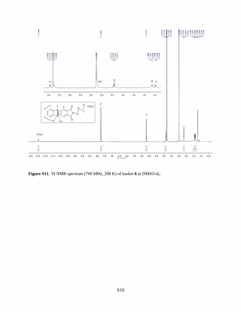
Figure S11. 1H NMR spectrum (700 MHz, 298 K) of basket 6 in DMSO-d6.

S17
Figure S12. 13C NMR (175 MHz, 298 K) of basket 6 in DMSO-d6.

S18
Figure S13. 1H-1H COSY NMR spectrum (700 MHz, 298 K) of basket 6 in DMSO-d6.

S19
Figure S14. 1H-13C HSQC NMR spectrum (700 MHz, 298 K) of basket 6 in DMSO-d6.

S20
Figure S15. (A) 1H NMR spectra (600 MHz, 298 K) of 0.1 mM solution of 16- (30 mM phosphate buffer at pH =
7.0) before and after 300 nm irradiation (Rayonet) for 55 minutes. (Bottom) 1H NMR spectrum (600 MHz, 298 K)
of 43- in DMSO-d6. (B) 1H NMR spectra (600 MHz, 298 K) of 0.1 mM solution of 36- (30 mM phosphate buffer at
pH = 7.0) before and after 300 nm irradiation (Rayonet) for 55 minutes. (Bottom) 1H NMR spectrum (600 MHz, 298
K) of 63- in DMSO-d6.
(A)
(B)
2.02.42.83.23.64.04.44.85.25.66.06.46.87.68.0 7.2
d (ppm)
16-
*
HE/F
HB/B’
HA/D/D’
HC/C’
43-
3CO2hn, 300 nm
~55 min
HA
HB
HC
HDHE/F
43-
HA
HB/B’
HC/C’
HD/D’HE/F
H2O
DM
SO
-d6
36-
63-
3CO2hn, 300 nm
~55 min
H2O
HD/D’
HC/C’HB/B’ HA
HE/E’
HF/F’HG/H
HB/B’HG/H HC/C’*
HA//F/F’HE/E’
0.51.01.52.02.53.04.04.55.05.56.06.58.0 7.5 7.0
d (ppm)
63-
HG/H
HF
HE
HDHC
HBHA HF
HE
3.5
1.52.53.54.55.56.57.58.59.5d (ppm)
HA
DM
SO
-d6
3.6 2.84.45.26.06.87.6d (ppm)
HA
HD
HC
HB
*
*
HE/F
HB/C
HD
*
HD/D’
HG/H

S21
Figure S16. 1H NMR spectra (600 MHz, 298.0 K) of basket 16- (in 30.0 mM phosphate buffer
with 20% D2O at pH = 7.0 ± 0.1) obtained upon an incremental dilution; note that solution
concentrations at which the spectra were taken are shown on the right.
0.07 mM
0.14 mM
0.28 mM
0.55 mM
1.1 mM

S22
Figure S17. (Top) DOSY NMR spectrum (600 MHz, 298 K) of 0.5 mM 16- in 30 mM phosphate
buffer (H2O:D2O = 9:1) at pH = 7.0. (Bottom) The change in intensity of resonance corresponding to
HB/B’ proton as a function of the field gradient g (G/cm) was obtained using the pulse field gradient
stimulated echo sequence with bipolar gradient pulse pair, 1 spoil gradient, 3-9-19 WATERGATE
solvent suppression (stebpgp1s19) pulse sequence and the data was fit to the Stejskal-Tanner equation
to give the value of diffusion coefficient D (m2/s); the process was completed for resonances HB/B’,
HC, HF and HG and the reported value of D is the arithmetic mean of 4 numerical values. The
hydrodynamic radius was computed using the Stokes-Einstein equation whereby the viscosity of 30.0
mM phosphate buffer at pH = 7.0 ± 0.1 is assumed to be similar to that of H2O:D2O = 9:1 (η = 0.91
mPa s at 298.1).

S23
Figure S18. 1H NMR spectra (600 MHz, 298.0 K) of basket 36- (in 30.0 mM phosphate buffer with 20% D2O
at pH = 7.0 ± 0.1) obtained upon an incremental dilution; note solution concentrations at which the spectra
were taken are shown on the left.
0.15 mM
0.3 mM
0.5 mM
1.0 mM
1.5 mM
2.0 mM
2.5 mM
3.19 mM

S24
Figure S19. (Top) DOSY NMR spectrum (600 MHz, 298 K) of 0.3 mM 36- in 30 mM phosphate
buffer (H2O:D2O = 9:1) at pH = 7.0. (Bottom) The change in intensity of resonance corresponding to
HA/A’ proton as a function of the field gradient g (G/cm) was obtained using the pulse field gradient
stimulated echo sequence with bipolar gradient pulse pair, 1 spoil gradient, 3-9-19 WATERGATE
solvent suppression (stebpgp1s19) pulse sequence and the data was fit to the Stejskal-Tanner equation
to give the value of diffusion coefficient D (m2/s); the process was completed for resonances HB/B’,
HC/C’, HD/D’, HE/E’, HH, HG and the reported value of D is the arithmetic mean of 6 numerical values.
The hydrodynamic radius was computed using the Stokes-Einstein equation whereby the viscosity of
30.0 mM phosphate buffer at pH = 7.0 ± 0.1 is assumed to be similar to that of H2O:D2O = 9:1 (η =
0.91 mPa s at 298.1). Note that signal at 2.1 ppm corresponds to residual acetic acid.

S25
Figure S20. The intensity distribution of scattered light as a function of hydrodynamic radii (DH)
particle size was obtained from Dynamic Light Scattering (DLS, 298 K) measurements of 1.0 mM
solution of 36- in 30.0 mM phosphate buffer at pH = 7.0 ± 0.1; DLS data were analyzed using the
viscosity of 0.8872 cP and refractive index (RI) = 1.330 (from pure water). (A) DH = 217.8 nm, DCR
= 6471.8 kcps, PDI = 0.262. (B) DH = 204.1 nm, DCR = 6277.8 kcps, PDI = 0.254. (C) DH = 213.8
nm, DCR = 6241.7 kcps, PDI = 0.266. The reported value of DH = 212 ± 7 nm is an arithmetic mean
of three measurements with the standard deviation as the error.
A B
C
S26
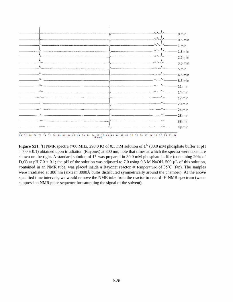
Figure S21. 1H NMR spectra (700 MHz, 298.0 K) of 0.1 mM solution of 16- (30.0 mM phosphate buffer at pH
= 7.0 ± 0.1) obtained upon irradiation (Rayonet) at 300 nm; note that times at which the spectra were taken are
shown on the right. A standard solution of 16- was prepared in 30.0 mM phosphate buffer (containing 20% of
D2O) at pH 7.0 ± 0.1; the pH of the solution was adjusted to 7.0 using 0.3 M NaOH. 500 µL of this solution,
contained in an NMR tube, was placed inside a Rayonet reactor at temperature of 35˚C (fan). The samples
were irradiated at 300 nm (sixteen 3000Å bulbs distributed symmetrically around the chamber). At the above
specified time intervals, we would remove the NMR tube from the reactor to record 1H NMR spectrum (water
suppression NMR pulse sequence for saturating the signal of the solvent).
0 min
0.5 min
1 min
1.5 min
2.5 min
3.5 min
5 min
6.5 min
8.5 min
11 min
14 min
17 min
20 min
24 min
28 min
38 min
48 min

S27
Figure S22. 1H NMR spectra (700 MHz, 298.0 K) of 0.1 mM solution of 36- (30.0 mM phosphate buffer at pH
= 7.0 ± 0.1) obtained upon irradiation (Rayonet) at 300 nm; note that times at which the spectra were taken are
shown on the right. A standard solution of 36- was prepared in 30.0 mM phosphate buffer (containing 20% of
D2O) at pH 7.0 ± 0.1; the pH of the solution was adjusted to 7.0 using 0.3 M NaOH. 500 µL of this solution,
contained in an NMR tube, was placed inside a Rayonet reactor at temperature of 35˚C (fan). The samples
were irradiated at 300 nm (sixteen 3000Å bulbs distributed symmetrically around the chamber). At the above
specified time intervals, we would remove the NMR tube from the reactor to record 1H NMR spectrum (water
suppression NMR pulse sequence for saturating the signal of the solvent).
0 min
1 min
2 min
4 min
6 min
8 min
11 min
15 min
20 min
30 min
40 min
50 min
60 min
70 min

S28
Figure S23. The intensity distribution of scattered light as a function of hydrodynamic radii (DH) was
obtained from Dynamic Light Scattering (DLS, 298 K) measurements of 1.0 mM solution of 43- in
30.0 mM phosphate buffer at pH = 7.0 ± 0.1; DLS data were analyzed using the viscosity of 0.8872
cP and refractive index (RI) = 1.330 (from pure water). (A) DH = 188.7 nm, DCR = 4056.7 kcps, PDI
= 0.37. (B) DH = 209.3 nm, DCR = 4239.2 kcps, PDI = 0.30. (C) DH = 189.5 nm, DCR = 4368.5
kcps, PDI = 0.38. The reported value of DH = 195 ± 12 nm is an arithmetic mean of three
measurements with the standard deviation as the error.
A B
C

S29
Figure S24. The intensity distribution of scattered light as a function of the particle size was obtained
from Dynamic Light Scattering (DLS, 298 K) measurements of 1.0 mM solution of 63- in 30.0 mM
phosphate buffer at pH = 7.0 ± 0.1; DLS data were analyzed using the viscosity of 0.8872 cP and
refractive index (RI) = 1.330 (from pure water). (A) average diameter = 219.7 nm, DCR = 1895.1
kcps, PDI = 0.55. (B) average diameter = 233.6 nm, DCR = 2066.2 kcps, PDI = 0.54. (C) average
diameter = 249.5 nm, DCR = 2222.1 kcps, PDI = 0.57. The reported value of DH = 235 ± 15 nm is an
arithmetic mean of three measurements with the standard deviation as the error.
A B
C
S30
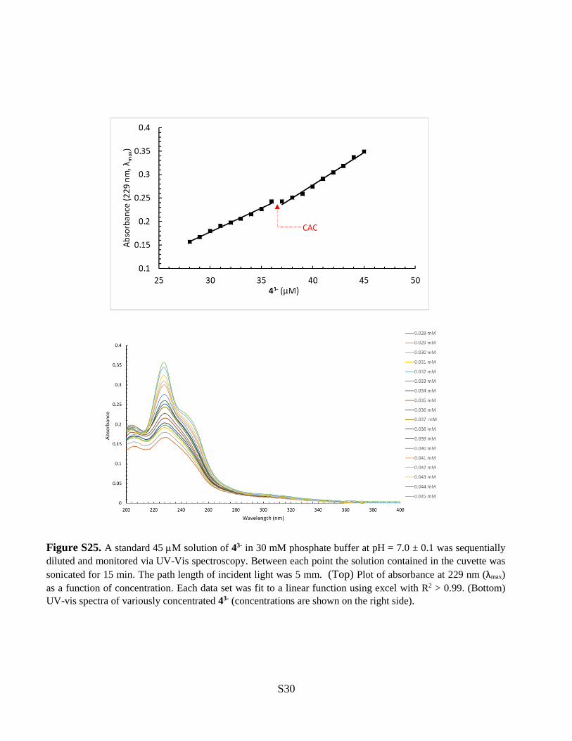
Figure S25. A standard 45 M solution of 43- in 30 mM phosphate buffer at pH = 7.0 ± 0.1 was sequentially
diluted and monitored via UV-Vis spectroscopy. Between each point the solution contained in the cuvette was
sonicated for 15 min. The path length of incident light was 5 mm. (Top) Plot of absorbance at 229 nm (λmax)
as a function of concentration. Each data set was fit to a linear function using excel with R2 > 0.99. (Bottom)
UV-vis spectra of variously concentrated 43- (concentrations are shown on the right side).

S31
Figure S26. A standard 15 M solution of 63- in 30 mM phosphate buffer at pH = 7.0 ± 0.1 was sequentially
diluted and monitored via UV-Vis spectroscopy to determine the critical aggregation concentration. The path
length of incident light was 1 cm. (Top) Plot of absorbance at 229 nm (λmax) as a function of concentration.
Each data set was fit to a linear function using excel with R2 > 0.99. (Bottom). UV-vis spectra of variously
concentrated 63- (concentrations are shown on the right side).
‘
0
0.2
0.4
0.6
0.8
1
1.2
1.4
1.6
0 2 4 6 8 10 12 14
Ab
sorb
ance
(2
29
nm
, λm
ax)
63- (µM)
CAC
-0.2
0
0.2
0.4
0.6
0.8
1
1.2
1.4
1.6
200 250 300 350 400
Ab
sorb
ance
Wavelength (nm)
0.015 mM
0.014 mM
0.013 mM
0.012 mM
0.011 mM
0.010 mM
0.009 mM
0.008 mM
0.007 mM
0.006 mM
0.005 mM
0.004 mM
0.003 mM

S32
Figure S27. (Top) 1H NMR spectra (700 MHz, 298 K) of 0.3 mM basket 16- obtained upon incremental
addition of DMMP (20.2 mM to neat) to this solution; see on the right for the number of molar equivalents of
DMMP. (Bottom) Nonlinear least-square analysis of 1H NMR binding data corresponding to the formation of
16-DMMP complex. The data, from two measurements (top and bottom), were each fit to 1:1 binding model
(SigmaPlot) revealing the formation of a binary complex with stability constants K = 13.9 ± 0.9 M-1 / K = 24 ±
1 M-1 and random distribution of residuals. The reported value K = 19 ± 7 M-1 is an arithmetic mean of two
measurements with the standard deviation.
746 eq
596 eq
446 eq
296 eq
196 eq
96 eq
48 eq
24 eq
12 eq
6 eq
3 eq
1.2 eq
0.9 eq
0.6 eq
0.3 eq
0 eq
S33
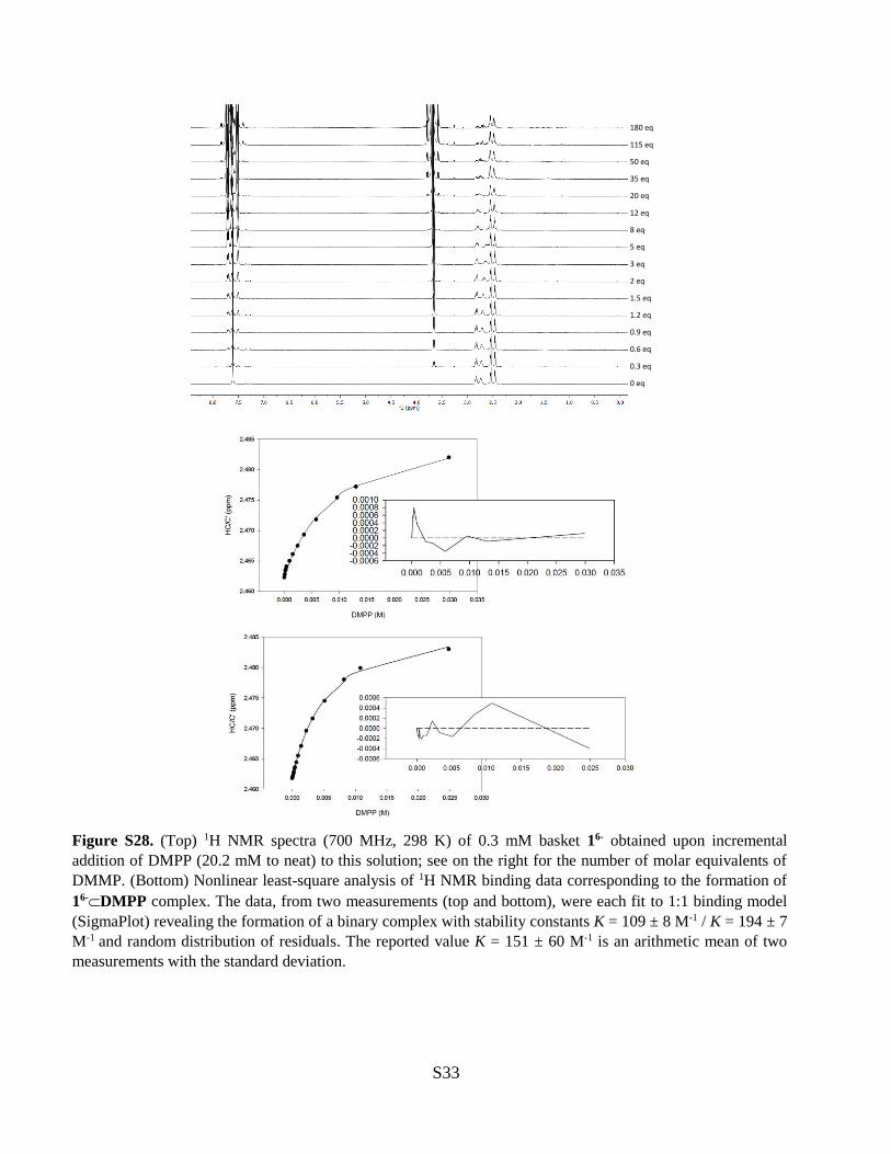
Figure S28. (Top) 1H NMR spectra (700 MHz, 298 K) of 0.3 mM basket 16- obtained upon incremental
addition of DMPP (20.2 mM to neat) to this solution; see on the right for the number of molar equivalents of
DMMP. (Bottom) Nonlinear least-square analysis of 1H NMR binding data corresponding to the formation of
16-DMPP complex. The data, from two measurements (top and bottom), were each fit to 1:1 binding model
(SigmaPlot) revealing the formation of a binary complex with stability constants K = 109 ± 8 M-1 / K = 194 ± 7
M-1 and random distribution of residuals. The reported value K = 151 ± 60 M-1 is an arithmetic mean of two
measurements with the standard deviation.
180 eq
115 eq
50 eq
35 eq
20 eq
12 eq
8 eq
5 eq
3 eq
2 eq
1.5 eq
1.2 eq
0.9 eq
0.6 eq
0.3 eq
0 eq

S34
Figure S29. (Top) 1H NMR spectra (700 MHz, 298 K) of 0.3 mM basket 26- obtained upon incremental
addition of DMPP (20.2 mM to neat) to this solution; see on the right for the number of molar equivalents of
DMMP. (Bottom) Nonlinear least-square analysis of 1H NMR binding data corresponding to the formation of
26-DMMP complex. The data, from two measurements (top and bottom), were each fit to 1:1 binding model
(SigmaPlot) revealing the formation of a binary complex with stability constants K = 34 ± 1 M-1 / K = 24.3 ±
0.6 M-1 and random distribution of residuals. The reported value K = 29 ± 7 M-1 is an arithmetic mean of two
measurements with the standard deviation.
0 eq
0.3 eq
0.6 eq
0.9 eq
1.2 eq
3.0 eq
6.0 eq
12.0 eq
24.0 eq
48.0 eq
96.0 eq
218.0 eq
340.0 eq
462.0 eq
584.0 eq
828.0 eq

S35
Figure S30. (Top) 1H NMR spectra (600 MHz, 298 K) of 0.3 mM basket 26- obtained upon incremental
addition of DMPP (20.6 mM to neat) to this solution; see on the right for the number of molar equivalents of
DMPP. (Bottom) Nonlinear least-square analysis of 1H NMR binding data corresponding to the formation of
26-DMPP complex. The data, from two measurements (top and bottom), were each fit to 1:1 binding model
(SigmaPlot) revealing the formation of a binary complex with stability constants K = 208 ± 16 M-1 / K = 218 ±
17 M-1 and random distribution of residuals. The reported value K = 213 ± 7 M-1 is an arithmetic mean of two
measurements with the standard deviation. Note that one can also fit the data to 1:2 stoichiometric model
(basket:DMPP = 1:2) albeit with a similar distribution of residuals to obtain K1 = 101 M-1/K2 = 14 M-1 and K1 =
138 M-1/K2 = 22 M-1.
0 eq
0.2 eq
0.4 eq
0.6 eq
0.8 eq
1.0 eq
1.5 eq
3.0 eq
5.0 eq
8.0 eq
11.0 eq
21.0 eq
41.0 eq
80.0 eq
167 eq
340 eq

S36
Figure S31. (Top) 1H NMR spectra (700 MHz, 298 K) of 0.3 mM basket 36- obtained upon incremental
addition of DMMP (20.2 mM to neat) to this solution; see on the right for the number of molar equivalents of
DMMP. (Bottom) Nonlinear least-square analysis of 1H NMR binding data corresponding to the formation of
36-DMMP complex. The data, from two measurements (top and bottom), were each fit to 1:1 binding model
(SigmaPlot) revealing the formation of a binary complex with the stability constants K = 62 ± 7 M-1 / K = 57 ±
4 M-1 and random distribution of residuals. The reported value K = 59 ± 4 M-1 is an arithmetic mean of two
measurements with the standard deviation.
683 eq
462 eq
340 eq
218 eq
96 eq
48 eq
24 eq
12 eq
6 eq
3 eq
1.2 eq
0.9 eq
0.6 eq
0.3 eq
0 eq

S37
Figure S32. (Top) 1H NMR spectra (600 MHz, 298 K) of 0.3 mM basket 36- obtained upon incremental
addition of DMPP (20.6 mM to neat) to this solution; see on the right for the number of molar equivalents of
DMPP. (Bottom) Nonlinear least-square analysis of 1H NMR binding data corresponding to the formation of
36-DMPP complex. The data, from two measurements (top and bottom), were each fit to 1:1 binding model
(SigmaPlot) revealing the formation of a binary complex with the stability constants K = 659 ± 57 M-1 / K =
775 ± 44 M-1 and a distribution of residuals that appears not fully randomized. The reported value K = 717 ± 82
M-1 is an arithmetic mean of two measurements with the standard deviation. When we fit the data to 1:2
stoichiometric model (basket:DMPP = 1:2), there was a somewhat better distribution of residuals and K1 = 566
M-1/K2 = 24 M-1 and K1 = 390 M-1/K2 = 40 M-1. With K1 > K2, the first binding event is dominating. If the
mean K1 = 478 M-1 value was subsequently incorporated instead of K = 717 ± 7 M-1 in Figure 4A, the observed
trend would remain the same.
181 eq
81 eq
61 eq
41 eq
21 eq
11 eq
7 eq
4 eq
2.5 eq
1.5 eq
1.0 eq
0.8 eq
0.6 eq
0.4 eq
0.2 eq
0 eq
S38
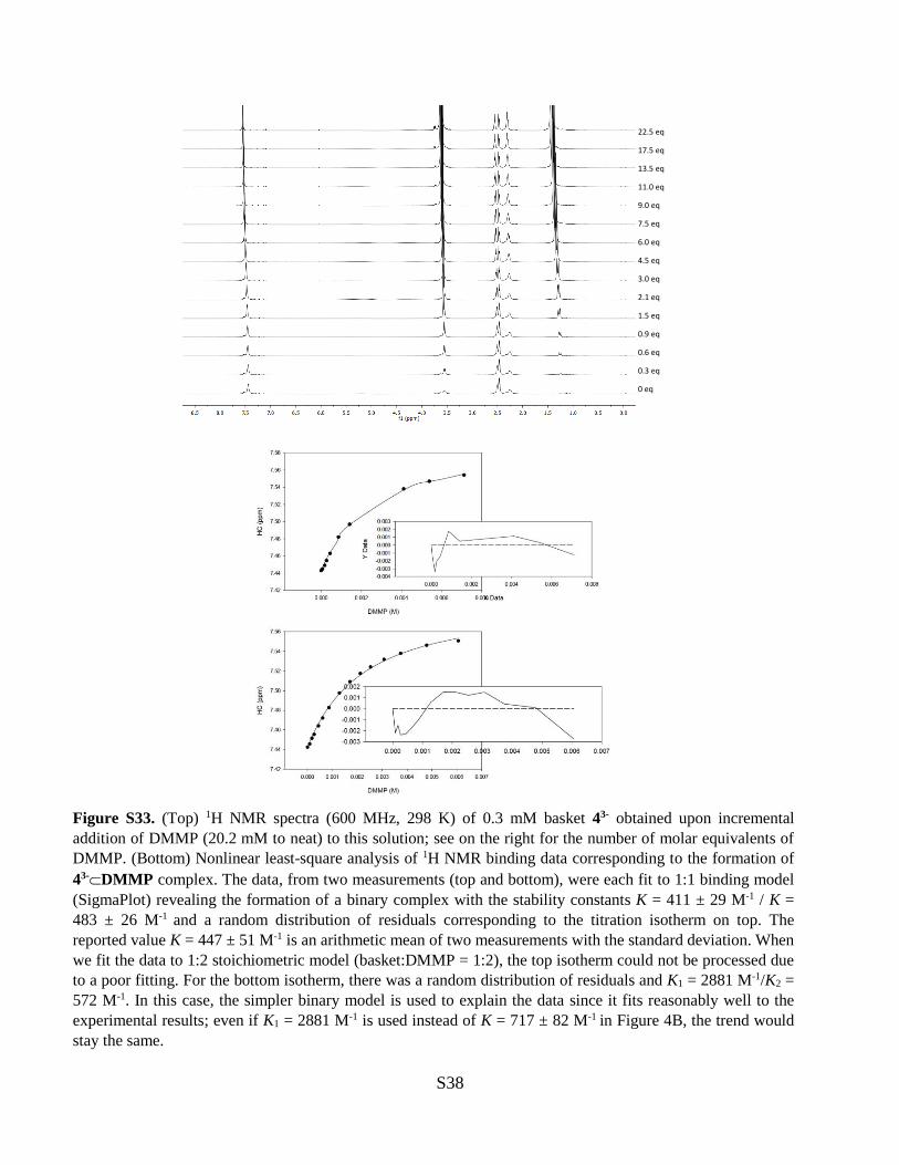
Figure S33. (Top) 1H NMR spectra (600 MHz, 298 K) of 0.3 mM basket 43- obtained upon incremental
addition of DMMP (20.2 mM to neat) to this solution; see on the right for the number of molar equivalents of
DMMP. (Bottom) Nonlinear least-square analysis of 1H NMR binding data corresponding to the formation of
43-DMMP complex. The data, from two measurements (top and bottom), were each fit to 1:1 binding model
(SigmaPlot) revealing the formation of a binary complex with the stability constants K = 411 ± 29 M-1 / K =
483 ± 26 M-1 and a random distribution of residuals corresponding to the titration isotherm on top. The
reported value K = 447 ± 51 M-1 is an arithmetic mean of two measurements with the standard deviation. When
we fit the data to 1:2 stoichiometric model (basket:DMMP = 1:2), the top isotherm could not be processed due
to a poor fitting. For the bottom isotherm, there was a random distribution of residuals and K1 = 2881 M-1/K2 =
572 M-1. In this case, the simpler binary model is used to explain the data since it fits reasonably well to the
experimental results; even if K1 = 2881 M-1 is used instead of K = 717 ± 82 M-1 in Figure 4B, the trend would
stay the same.
22.5 eq
17.5 eq
13.5 eq
11.0 eq
9.0 eq
7.5 eq
6.0 eq
4.5 eq
3.0 eq
2.1 eq
1.5 eq
0.9 eq
0.6 eq
0.3 eq
0 eq
S39
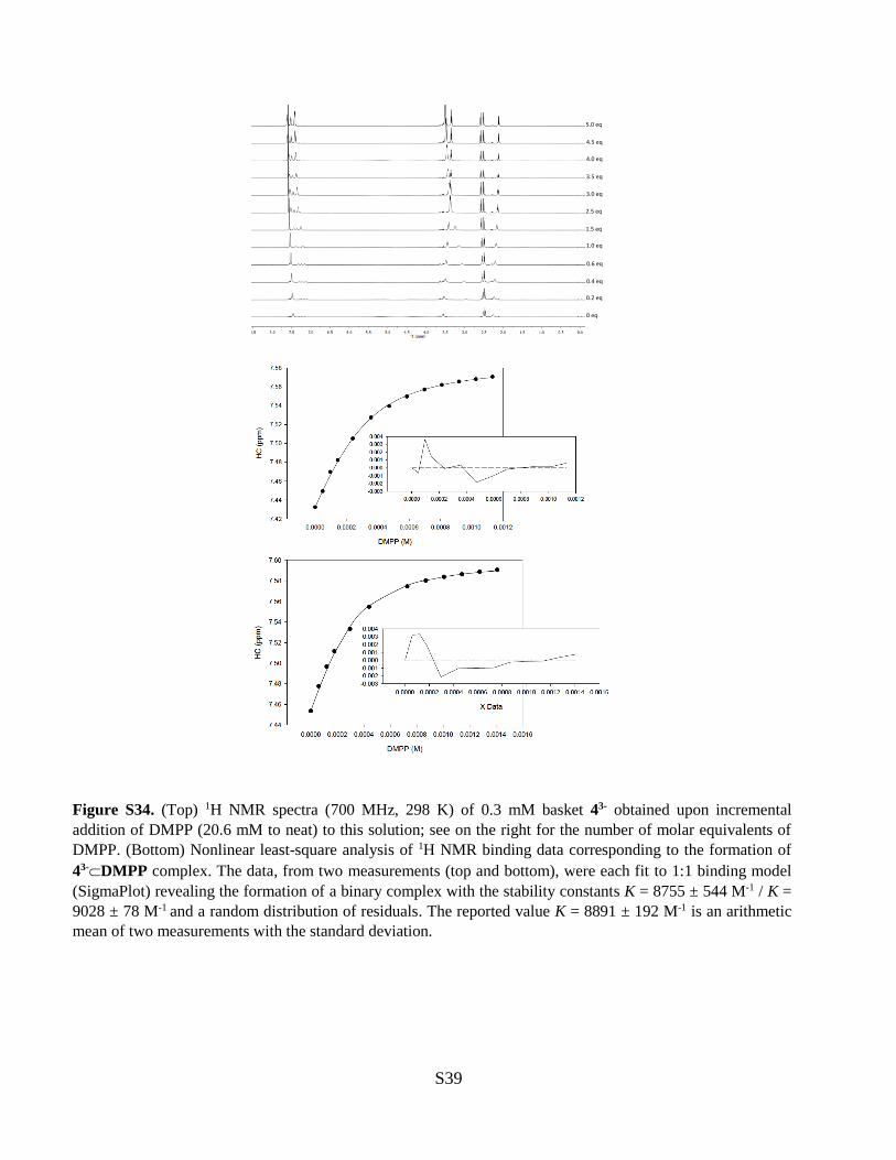
Figure S34. (Top) 1H NMR spectra (700 MHz, 298 K) of 0.3 mM basket 43- obtained upon incremental
addition of DMPP (20.6 mM to neat) to this solution; see on the right for the number of molar equivalents of
DMPP. (Bottom) Nonlinear least-square analysis of 1H NMR binding data corresponding to the formation of
43-DMPP complex. The data, from two measurements (top and bottom), were each fit to 1:1 binding model
(SigmaPlot) revealing the formation of a binary complex with the stability constants K = 8755 ± 544 M-1 / K =
9028 ± 78 M-1 and a random distribution of residuals. The reported value K = 8891 ± 192 M-1 is an arithmetic
mean of two measurements with the standard deviation.
0 eq
0.2 eq
0.4 eq
0.6 eq
1.0 eq
1.5 eq
2.5 eq
3.0 eq
3.5 eq
4.0 eq
4.5 eq
5.0 eq

S40
Figure S35. (Top) 1H NMR spectra (600 MHz, 298 K) of 0.3 mM basket 53- obtained upon incremental
addition of DMMP (20.2 mM to neat) to this solution; see on the right for the number of molar equivalents of
DMMP. (Bottom) Nonlinear least-square analysis of 1H NMR binding data corresponding to the formation of
53-DMMP complex. The data, from two measurements (top and bottom), were each fit to 1:1 binding model
(SigmaPlot) revealing the formation of a binary complex with the stability constants K = 385 ± 15 M-1 / K =
238 ± 9 M-1 and a random distribution of residuals. The reported value K = 311 ± 99 M-1 is an arithmetic mean
of two measurements with the standard deviation.
0 eq
0.3 eq
0.6 eq
0.9 eq
2.4 eq
1.2 eq
3.6 eq
4.8 eq
6.8 eq
8.8 eq
10.8 eq
13.3 eq
15.8 eq
18.8 eq
21.8 eq
25.3 eq
30.3 eq
40.3 eq
55.3 eq

S41
Figure S36. (Top) 1H NMR spectra (600 MHz, 298 K) of 0.3 mM basket 53- obtained upon incremental
addition of DMPP (20.6 mM to neat) to this solution; see on the right for the number of molar equivalents of
DMPP. (Bottom) Nonlinear least-square analysis of 1H NMR binding data corresponding to the formation of
53-DMPP complex. The data, from three measurements, were each fit to 1:1 binding model (SigmaPlot)
revealing the formation of a binary complex with stability constants K = 3742 ± 65 M-1 / K = 3675 ± 102 M-1/
K = 4412 ± 68 M-1 and a random distribution of residuals corresponding to the last data set. The reported value
K = 3943 ± 407 M-1 is an arithmetic mean of three measurements with the standard deviation.
16 eq
12.8 eq
9.6 eq
6.4 eq
3.2 eq
1.6 eq
0.8 eq
0.4 eq
0.2 eq
0 eq
S42
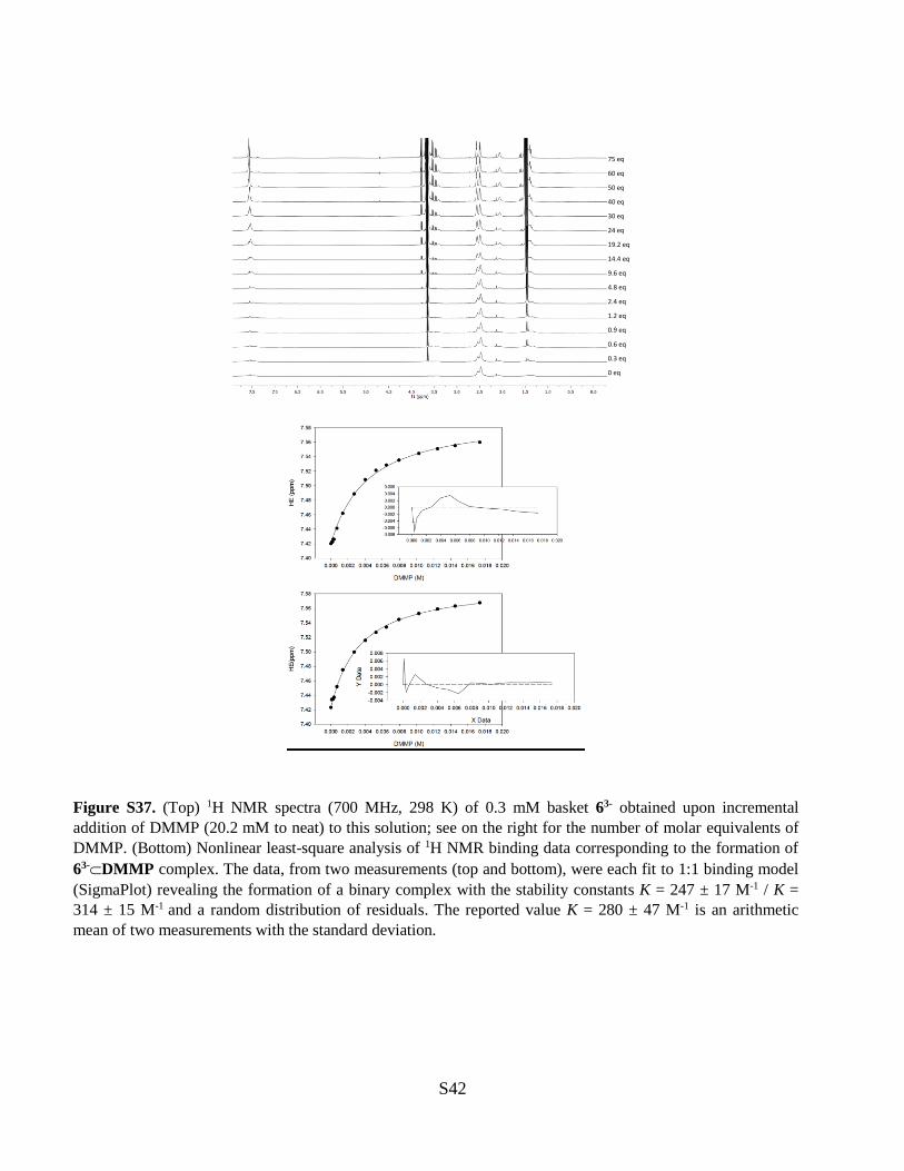
Figure S37. (Top) 1H NMR spectra (700 MHz, 298 K) of 0.3 mM basket 63- obtained upon incremental
addition of DMMP (20.2 mM to neat) to this solution; see on the right for the number of molar equivalents of
DMMP. (Bottom) Nonlinear least-square analysis of 1H NMR binding data corresponding to the formation of
63-DMMP complex. The data, from two measurements (top and bottom), were each fit to 1:1 binding model
(SigmaPlot) revealing the formation of a binary complex with the stability constants K = 247 ± 17 M-1 / K =
314 ± 15 M-1 and a random distribution of residuals. The reported value K = 280 ± 47 M-1 is an arithmetic
mean of two measurements with the standard deviation.
75 eq
60 eq
50 eq
40 eq
30 eq
24 eq
19.2 eq
14.4 eq
9.6 eq
4.8 eq
2.4 eq
1.2 eq
0.9 eq
0.6 eq
0.3 eq
0 eq

S43
Figure S38. (Top) 1H NMR spectra (700 MHz, 298 K) of 0.3 mM basket 63- obtained upon incremental
addition of DMPP (20.6 mM to neat) to this solution; see on the right for the number of molar equivalents of
DMPP. (Bottom) Nonlinear least-square analysis of 1H NMR binding data corresponding to the formation of
63-DMPP complex. The data, from two measurements (top and bottom), were each fit to 1:1 binding model
(SigmaPlot) revealing the formation of a binary complex with the stability constants K = 2498 ± 287 M-1 / K =
2596 ± 234 M-1 and a random distribution of residuals. The reported value K = 2547 ± 69 M-1 is an arithmetic
mean of two measurements with the standard deviation.
0 eq
0.2 eq
0.4 eq
0.6 eq
0.8 eq
1.0 eq
1.2 eq
1.6 eq
2.0 eq
2.5 eq
3.5 eq
5.0 eq
6.5 eq
9.0 eq
12.0 eq
15.0 eq
18.0 eq
21.0 eq

S44
Figure S39. Cryo-TEM images of (top three) 1.0 mM solution of 43- in 30 mM phosphate buffer at pH = 7.0
and (bottom three) 1.0 mM solution of 43- in 30 mM phosphate buffer at pH = 7.0 with ten molar equivalents of
DMPP. To determine the size of nanoparticles, we randomly chose ten “dots” to obtain their length and height
followed by determining the arithmetic mean and standard deviation of such twenty values (see Figure 3B in
the main text).
P
OCH3
H3CO
O
10 mol eq DMPP
30 mM PBSpH = 7.0

S45
Figure S40. Cryo-TEM images of (top three) 1.0 mM solution of 63- in 30 mM phosphate buffer at pH = 7.0
and (bottom three) 1.0 mM solution of 63- in 30 mM phosphate buffer at pH = 7.0 with ten molar equivalents of
DMPP. To determine the size of nanoparticles, we randomly chose ten “dots” to obtain their length and height
followed by determining the arithmetic mean and standard deviation of such twenty values (see Figure 3B in
the main text).
P
OCH3
H3CO
O
10 mol eq DMPP
30 mM PBSpH = 7.0

S46
Figure S41. Cryo-TEM images of (top three) 1.0 mM solution of 53- in 30 mM phosphate buffer at pH = 7.0
and (bottom) 1.0 mM solution of 53- in 30 mM phosphate buffer at pH = 7.0 with ten molar equivalents of
DMPP. To determine the size of nanoparticles, we randomly chose ten “dots” to obtain their length and height
followed by determining the arithmetic mean and standard deviation of such twenty values (see Figure 3B in
the main text).
P
OCH3
H3CO
O
10 mol eq DMPP
30 mM PBSpH = 7.0

S47
Figure S42. Conventional TEM images of (top two) 1.0 mM solution of 43- in 30 mM phosphate buffer at pH
= 7.0 and (bottom two) 1.0 mM solution of 43- in 30 mM phosphate buffer at pH = 7.0 with ten molar
equivalents of DMPP.
30 mM PBS pH = 7

S48
Figure S43. Conventional TEM images of (top two) 1.0 mM solution of 63- in 30 mM phosphate buffer at pH
= 7.0 and (bottom two) 1.0 mM solution of 63- in 30 mM phosphate buffer at pH = 7.0 with ten molar
equivalents of DMPP.

S49
Figure S44. 1H NMR spectra (700 MHz, 298.0 K) of 0.8 mM solution of 16- with 0.4 molar equivalents
of DMPP (30.0 mM phosphate buffer at pH = 7.0 ± 0.1) obtained upon irradiation at 300 nm; note that
times at which the spectra were taken are shown on the right. A standard solution of 16- was prepared in
30.0 mM phosphate buffer (containing 20% of D2O) at pH 7.0 ± 0.1; the pH of the solution was adjusted
to 7.0 using 0.3 M NaOH. 500 µL of this solution, contained in an NMR tube, was placed inside a
Rayonet reactor to maintain a constant temperature of 35˚C (fan). The samples were irradiated at 300 nm
(sixteen 3000Å bulbs distributed symmetrically around the chamber). At certain time intervals, we would
remove the NMR tube from the reactor to record 1H NMR spectrum (water suppression NMR pulse
sequence for saturating the signal of the solvent). Note: the methoxy and an aromatic resonance of DMPP
are highlighted with a red asterisk at each time point.
0 min
8 min
16 min
24 min
32 min
44 min
64 min
84 min
10 %
83 %
Encapsulation Promoted with light

S50
Figure S45. 1H NMR spectra (600 MHz, 298 K) of, from top to bottom: (a) 0.2 mM DMPP in PBS buffer
at pH = 7.0, (b) 0.2 mM DMPP in Surine, (c) 0.3 mM 43- in 30 mM PBS buffer at pH = 7.0 containing
0.2 mM DMPP and (d) 0.3 mM 43- in Surine containing 0.2 mM DMPP.
C6H5
OCH3
(A)
(B)
(C)
(D)
* urea
* creatinine

S51
Computational Studies
The Monte-Carlo (MC) conformational sampling of 16- and 36- was completed with the Maestro
suite (Schrodinger) using OPLS3 molecular mechanics (MM) force field in implicit H2O solvent.
For each search, we used systematic torsional sampling method with 200 steps per rotatable bond
and 50,000 steps overall. The energy window for saving structures was set to 50 kJ/mol.
Figure S46. For capsule 16-, the MCMM search gave 100 unique conformers of which 10 within
5 kcal/mol are shown on the left. For capsule 36-, the MCMM search gave 5019 unique
conformers of which 33 within 2 kcal/mol are shown on the right.
Figure S47. To estimate hydrodynamic radii rH of 16-, 26- and 36- (Figure 3B) we used distance d
between terminal carboxylates of fully extended baskets (MCMM calculation results, Figure
S42). Following, we used the following equation cos 30º = (d/2)/rH to calculate rH, as shown in
Figure 3B.
d
rH
30º
d/2
cos 30º = (d/2)/rH
d = 18 A for 16-
d = 19 A for 26-
d = 20 A for 36-

S52
Reference
(1) Border, S. E.; Pavlović, R. Z.; Zhiquan, L.; Badjić, J. D. Removal of Nerve Agent
Simulants from Water Using Light-Responsive Molecular Baskets. J. Am. Chem. Soc.
2017, 139 (51).