phosphor modeling in lighttools - synopsys€¦ · · 2018-04-14phosphor modeling in lighttools...

White Paper

Phosphor Modeling in LightToolsEnsuring Accurate White LED Models

Author

Michael Zollers

Applications

Engineer, LightTools

and CODE V, Optical

Solutions Group,

Synopsys, Inc.

Phosphors exhibit photoluminescence, the process by which a material absorbs light of a specific

spectral range and re-emits light of another spectral range with longer wavelengths. Because of the

increased availability of phosphor-based white light-emitting diodes, the use of phosphors is increasingly

prevalent in illumination design. To ensure that simulations for such illumination designs are accurate, it is

important to accurately model the optical effects of phosphors. To describe how phosphors are modeled

in LightTools, this paper explains how LightTools inputs correlate to theoretical models, as well as how to

obtain the necessary data.

Phosphor 101The law of conservation of energy states that when light is absorbed by a material, the energy must go

somewhere. In most materials, the energy is converted to heat; however, in photoluminescent materials

part of the energy is converted to heat, while the rest is converted to longer wavelength light. One way to

visualize this concept is to consider an electron band diagram, as shown in Figure 1.

Figure 1: Electron band diagram

Electrons orbiting an atom’s nucleus have discrete energy levels, and a similar energy structure exists in

many materials. However, instead of the discrete energy levels found in atoms, the molecular structure

results in energy bands for the electrons. The valence band, a lower, steady-state energy level, is

represented in Figure 1 as the baseline. The conduction band, the higher energy state at which electrons

are free to flow in the material, is represented as the higher level in the diagram. The vertical axis of the

chart represents the energy level, with higher energy levels toward the top of the chart.

The distance between the two energy levels, EG, known as the bandgap energy, is determined by the

atomic configuration of the material. Phosphor designers typically add impurities to a phosphor crystal (a

practice known as “doping”) to adjust the bandgap to accept and emit particular wavelengths of light.

January 2011

Conduction band

Valence band

E

e- e-e-

EG

Phosphor Modeling in LightTools 2

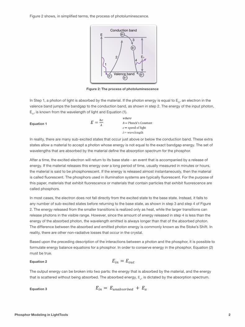
Figure 2 shows, in simplified terms, the process of photoluminescence.

Figure 2: The process of photoluminescence

In Step 1, a photon of light is absorbed by the material. If the photon energy is equal to EG, an electron in the

valence band jumps the bandgap to the conduction band, as shown in step 2. The energy of the input photon,

Ein, is known from the wavelength of light and Equation (1).

In reality, there are many sub-excited states that occur just above or below the conduction band. These extra

states allow a material to accept a photon whose energy is not equal to the exact bandgap energy. The set of

wavelengths that are absorbed by the material define the absorption spectrum for the phosphor.

After a time, the excited electron will return to its base state - an event that is accompanied by a release of

energy. If the material releases this energy over a long period of time, usually measured in minutes or hours,

the material is said to be phosphorescent. If the energy is released almost instantaneously, then the material

is called fluorescent. The phosphors used in illumination systems are typically fluorescent. For the purpose of

this paper, materials that exhibit fluorescence or materials that contain particles that exhibit fluorescence are

called phosphors.

In most cases, the electron does not fall directly from the excited state to the base state. Instead, it falls to

any number of sub-excited states before returning to the base state, as shown in step 3 and step 4 of Figure

2. The energy released from the smaller transitions is realized only as heat, while the larger transitions can

release photons in the visible range. However, since the amount of energy released in step 4 is less than the

energy of the absorbed photon, the wavelength emitted is always longer than that of the absorbed photon.

The difference between the absorbed and emitted photon energy is commonly known as the Stoke’s Shift. In

reality, there are other non-radiative losses that occur in the crystal.

Based upon the preceding description of the interactions between a photon and the phosphor, it is possible to

formulate energy balance equations for a phosphor. In order to conserve energy in the phosphor, Equation (2)

must be true.

The output energy can be broken into two parts: the energy that is absorbed by the material, and the energy

that is scattered without being absorbed. The absorbed energy, Eα, is dictated by the absorption spectrum.

Equation 1

Equation 2

Equation 3

Conduction band

Valence band

E

e- e-e-

EG

e-

e-

1

2

3

4


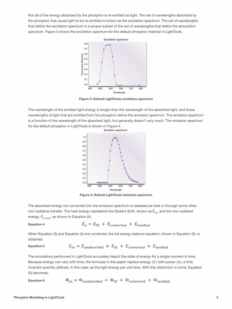
Not all of the energy absorbed by the phosphor is re-emitted as light. The set of wavelengths absorbed by

the phosphor that cause light to be re-emitted is known as the excitation spectrum. The set of wavelengths

that define the excitation spectrum is a proper subset of the set of wavelengths that define the absorption

spectrum. Figure 3 shows the excitation spectrum for the default phosphor material in LightTools.

Figure 3: Default LightTools excitation spectrum

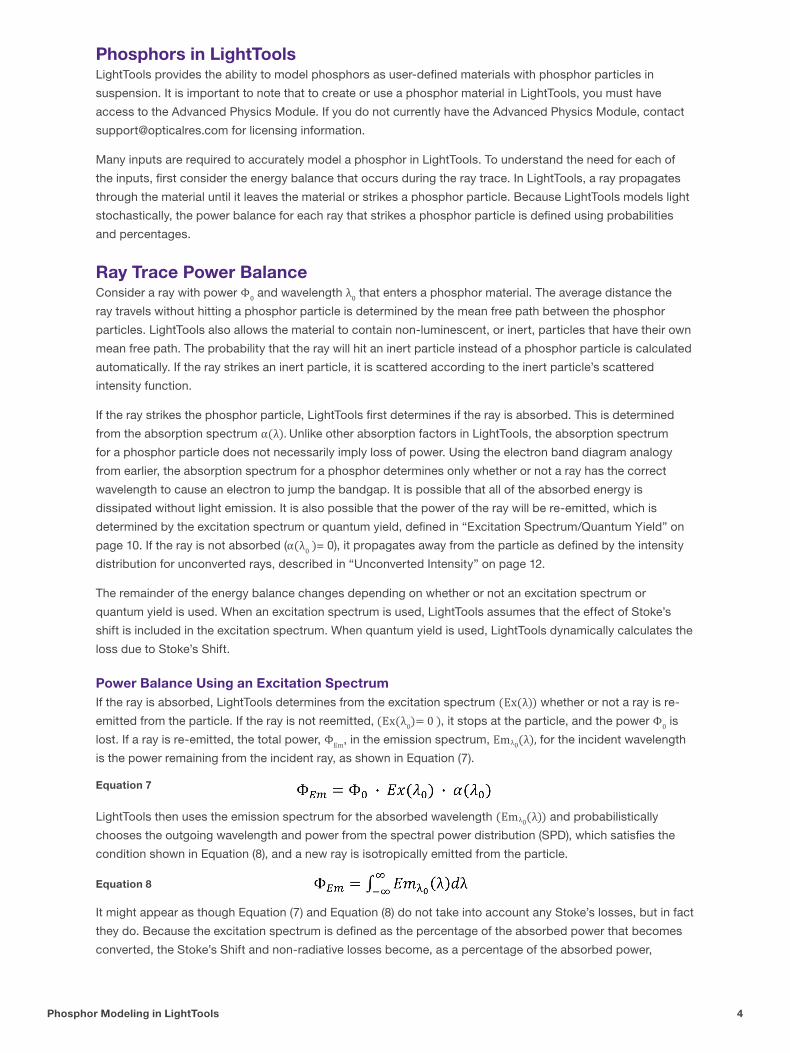
The wavelength of the emitted light energy is longer than the wavelength of the absorbed light, and those

wavelengths of light that are emitted from the phosphor define the emission spectrum. The emission spectrum

is a function of the wavelength of the absorbed light, but generally doesn’t vary much. The emission spectrum

for the default phosphor in LightTools is shown in Figure 4.

Figure 4: Default LightTools emission spectrum

The absorbed energy not converted into the emission spectrum is released as heat or through some other

non-radiative transfer. The heat energy represents the Stoke’s Shift, shown as ESS, and the non-radiated

energy, EnonRad, as shown in Equation (4).

When Equation (3) and Equation (4) are combined, the full energy balance equation, shown in Equation (5), is

obtained.

The simulations performed in LightTools accurately depict the state of energy for a single moment in time.

Because energy can vary with time, the formulas in this paper replace energy (E) with power (Φ), a time

invariant quantity defined, in this case, as the light energy per unit time. With this distinction in mind, Equation

(5) becomes:

Equation 4

Equation 5

Equation 6

Con

vers

ion

ellic

ienc

y

Wavelength

0.8

0.7

0.6

0.5

0.4

0.3

0.2

0.1

0.0

Excitation spectrum

300 400 500 600 700 800

Wavelength

1.0

0.9

0.8

0.7

0.6

0.5

0.4

0.3

0.2

0.1

0.0

300 400 500 600 700 800

Emission spectrum


Phosphors in LightToolsLightTools provides the ability to model phosphors as user-defined materials with phosphor particles in

suspension. It is important to note that to create or use a phosphor material in LightTools, you must have

access to the Advanced Physics Module. If you do not currently have the Advanced Physics Module, contact

[email protected] for licensing information.

Many inputs are required to accurately model a phosphor in LightTools. To understand the need for each of

the inputs, first consider the energy balance that occurs during the ray trace. In LightTools, a ray propagates

through the material until it leaves the material or strikes a phosphor particle. Because LightTools models light

stochastically, the power balance for each ray that strikes a phosphor particle is defined using probabilities

and percentages.

Ray Trace Power BalanceConsider a ray with power Φ0 and wavelength λ0 that enters a phosphor material. The average distance the

ray travels without hitting a phosphor particle is determined by the mean free path between the phosphor

particles. LightTools also allows the material to contain non-luminescent, or inert, particles that have their own

mean free path. The probability that the ray will hit an inert particle instead of a phosphor particle is calculated

automatically. If the ray strikes an inert particle, it is scattered according to the inert particle’s scattered

intensity function.

If the ray strikes the phosphor particle, LightTools first determines if the ray is absorbed. This is determined

from the absorption spectrum α(λ). Unlike other absorption factors in LightTools, the absorption spectrum

for a phosphor particle does not necessarily imply loss of power. Using the electron band diagram analogy

from earlier, the absorption spectrum for a phosphor determines only whether or not a ray has the correct

wavelength to cause an electron to jump the bandgap. It is possible that all of the absorbed energy is

dissipated without light emission. It is also possible that the power of the ray will be re-emitted, which is

determined by the excitation spectrum or quantum yield, defined in “Excitation Spectrum/Quantum Yield” on

page 10. If the ray is not absorbed (α(λ0 )= 0), it propagates away from the particle as defined by the intensity

distribution for unconverted rays, described in “Unconverted Intensity” on page 12.

The remainder of the energy balance changes depending on whether or not an excitation spectrum or

quantum yield is used. When an excitation spectrum is used, LightTools assumes that the effect of Stoke’s

shift is included in the excitation spectrum. When quantum yield is used, LightTools dynamically calculates the

loss due to Stoke’s Shift.

Power Balance Using an Excitation SpectrumIf the ray is absorbed, LightTools determines from the excitation spectrum (Ex(λ)) whether or not a ray is re-

emitted from the particle. If the ray is not reemitted, (Ex(λ0)= 0 ), it stops at the particle, and the power Φ0 is

lost. If a ray is re-emitted, the total power, ΦEm, in the emission spectrum, Emλ0(λ), for the incident wavelength

is the power remaining from the incident ray, as shown in Equation (7).

LightTools then uses the emission spectrum for the absorbed wavelength (Emλ0(λ)) and probabilistically

chooses the outgoing wavelength and power from the spectral power distribution (SPD), which satisfies the

condition shown in Equation (8), and a new ray is isotropically emitted from the particle.

It might appear as though Equation (7) and Equation (8) do not take into account any Stoke’s losses, but in fact

they do. Because the excitation spectrum is defined as the percentage of the absorbed power that becomes

converted, the Stoke’s Shift and non-radiative losses become, as a percentage of the absorbed power,

Equation 7

Equation 8


1 –Ex(λ). LightTools uses the excitation spectrum as a multiplicative factor; therefore, the ray’s power is

reduced by the Stoke’s Shift and non-radiative losses.

Power Balance using Quantum YieldIn this case, once the ray is absorbed by the phosphor particle, LightTools uses the quantum yield (QY(λ)) to

determine if the ray is re-emitted. As with the excitation spectrum, if QY(λ) = 0, the ray stops at the particle

and its power is lost. Otherwise, LightTools probabilistically chooses an outgoing wavelength (λ1) from the

emission spectrum for the incoming wavelength. The power in the outgoing ray (Φ1) is determined by the

relation shown in Equation (9).

Creating a Phosphor Material in the LightTools User InterfaceThe following three steps are used to create a phosphor material in LightTools.

1. Create a new User Material.

2. Add one or more Phosphor Particles to the new user material.

3. Specify the physical and optical properties of each of the phosphor particles.

Each of these steps will be elaborated upon in the subsequent sections.

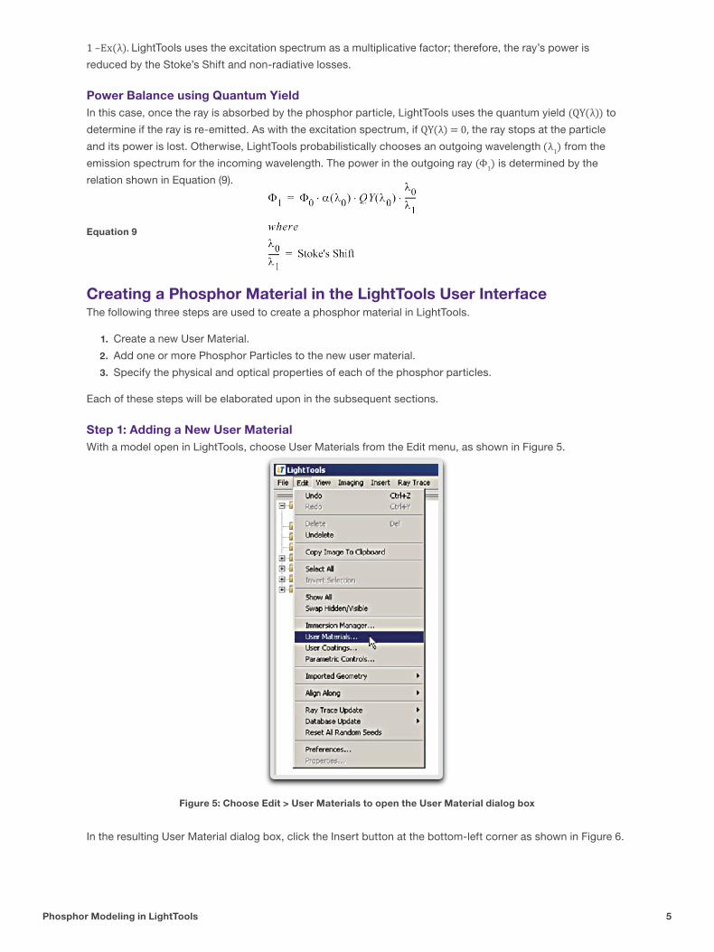
Step 1: Adding a New User MaterialWith a model open in LightTools, choose User Materials from the Edit menu, as shown in Figure 5.

Figure 5: Choose Edit > User Materials to open the User Material dialog box

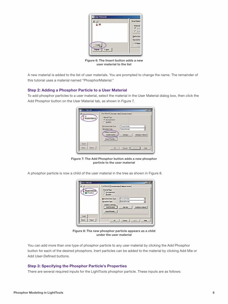
In the resulting User Material dialog box, click the Insert button at the bottom-left corner as shown in Figure 6.

Equation 9


Figure 6: The Insert button adds a new user material to the list

A new material is added to the list of user materials. You are prompted to change the name. The remainder of

this tutorial uses a material named “PhosphorMaterial.”

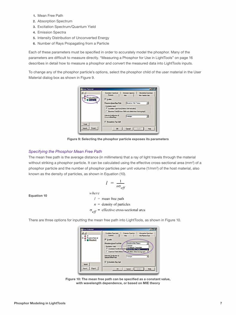
Step 2: Adding a Phosphor Particle to a User MaterialTo add phosphor particles to a user material, select the material in the User Material dialog box, then click the

Add Phosphor button on the User Material tab, as shown in Figure 7.

Figure 7: The Add Phosphor button adds a new phosphor particle to the user material

A phosphor particle is now a child of the user material in the tree as shown in Figure 8.

Figure 8: The new phosphor particle appears as a child under the user material

You can add more than one type of phosphor particle to any user material by clicking the Add Phosphor

button for each of the desired phosphors. Inert particles can be added to the material by clicking Add Mie or

Add User-Defined buttons.

Step 3: Specifying the Phosphor Particle’s PropertiesThere are several required inputs for the LightTools phosphor particle. These inputs are as follows:


1. Mean Free Path

2. Absorption Spectrum

3. Excitation Spectrum/Quantum Yield

4. Emission Spectra

5. Intensity Distribution of Unconverted Energy

6. Number of Rays Propagating from a Particle

Each of these parameters must be specified in order to accurately model the phosphor. Many of the

parameters are difficult to measure directly. “Measuring a Phosphor for Use in LightTools” on page 16

describes in detail how to measure a phosphor and convert the measured data into LightTools inputs.

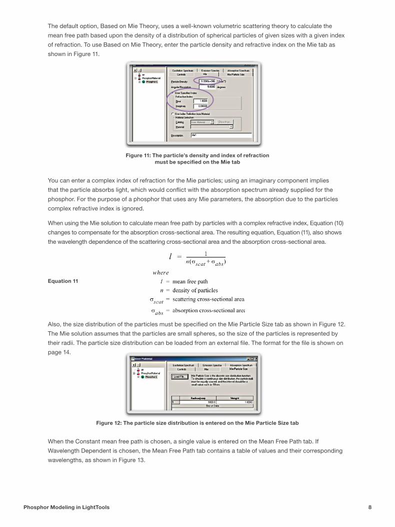
To change any of the phosphor particle’s options, select the phosphor child of the user material in the User

Material dialog box as shown in Figure 9.

Figure 9: Selecting the phosphor particle exposes its parameters

Specifying the Phosphor Mean Free PathThe mean free path is the average distance (in millimeters) that a ray of light travels through the material

without striking a phosphor particle. It can be calculated using the effective cross-sectional area (mm2) of a

phosphor particle and the number of phosphor particles per unit volume (1/mm3) of the host material, also

known as the density of particles, as shown in Equation (10).

There are three options for inputting the mean free path into LightTools, as shown in Figure 10.

Figure 10: The mean free path can be specified as a constant value, with wavelength dependence, or based on MIE theory

Equation 10


The default option, Based on Mie Theory, uses a well-known volumetric scattering theory to calculate the

mean free path based upon the density of a distribution of spherical particles of given sizes with a given index

of refraction. To use Based on Mie Theory, enter the particle density and refractive index on the Mie tab as

shown in Figure 11.

Figure 11: The particle’s density and index of refraction must be specified on the Mie tab

You can enter a complex index of refraction for the Mie particles; using an imaginary component implies

that the particle absorbs light, which would conflict with the absorption spectrum already supplied for the

phosphor. For the purpose of a phosphor that uses any Mie parameters, the absorption due to the particles

complex refractive index is ignored.

When using the Mie solution to calculate mean free path by particles with a complex refractive index, Equation (10)

changes to compensate for the absorption cross-sectional area. The resulting equation, Equation (11), also shows

the wavelength dependence of the scattering cross-sectional area and the absorption cross-sectional area.

Also, the size distribution of the particles must be specified on the Mie Particle Size tab as shown in Figure 12.

The Mie solution assumes that the particles are small spheres, so the size of the particles is represented by

their radii. The particle size distribution can be loaded from an external file. The format for the file is shown on

page 14.

Figure 12: The particle size distribution is entered on the Mie Particle Size tab

When the Constant mean free path is chosen, a single value is entered on the Mean Free Path tab. If

Wavelength Dependent is chosen, the Mean Free Path tab contains a table of values and their corresponding

wavelengths, as shown in Figure 13.

Equation 11


Figure 13: The mean free path can have wavelength dependence

The data can be entered manually, or an external text file can be used. The format for the text file is given on

page 14.

A Density Scale Factor can be entered on this tab to change the absolute values of all of the mean free paths

without shifting the relative shape of the curve. The scale factor is applied as if the particle density is being

changed. From Equation (10), the mean free path and the particle density have an inverse relationship; assuming

a constant particle size, if the density is doubled, the mean free path is halved. This allows you to change or

optimize on the density, which is easier to measure, while using a wavelength-dependent mean free path.

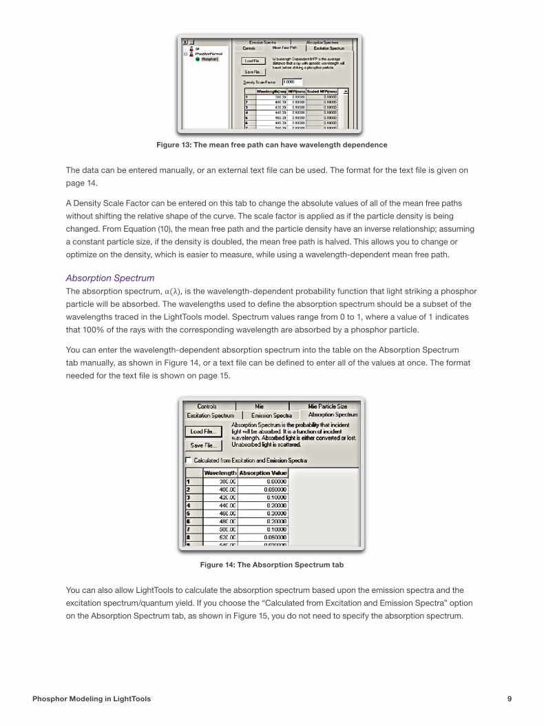
Absorption SpectrumThe absorption spectrum, α(λ), is the wavelength-dependent probability function that light striking a phosphor

particle will be absorbed. The wavelengths used to define the absorption spectrum should be a subset of the

wavelengths traced in the LightTools model. Spectrum values range from 0 to 1, where a value of 1 indicates

that 100% of the rays with the corresponding wavelength are absorbed by a phosphor particle.

You can enter the wavelength-dependent absorption spectrum into the table on the Absorption Spectrum

tab manually, as shown in Figure 14, or a text file can be defined to enter all of the values at once. The format

needed for the text file is shown on page 15.

Figure 14: The Absorption Spectrum tab

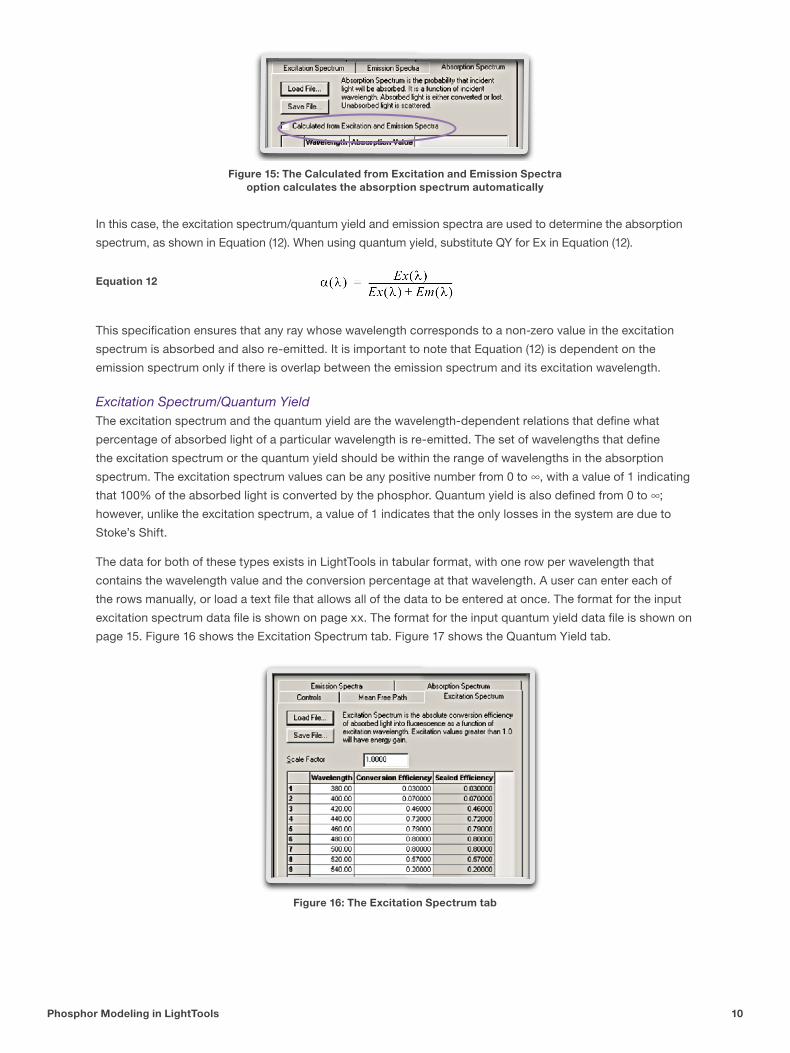
You can also allow LightTools to calculate the absorption spectrum based upon the emission spectra and the

excitation spectrum/quantum yield. If you choose the “Calculated from Excitation and Emission Spectra” option

on the Absorption Spectrum tab, as shown in Figure 15, you do not need to specify the absorption spectrum.


Figure 15: The Calculated from Excitation and Emission Spectra option calculates the absorption spectrum automatically

In this case, the excitation spectrum/quantum yield and emission spectra are used to determine the absorption

spectrum, as shown in Equation (12). When using quantum yield, substitute QY for Ex in Equation (12).

This specification ensures that any ray whose wavelength corresponds to a non-zero value in the excitation

spectrum is absorbed and also re-emitted. It is important to note that Equation (12) is dependent on the

emission spectrum only if there is overlap between the emission spectrum and its excitation wavelength.

Excitation Spectrum/Quantum YieldThe excitation spectrum and the quantum yield are the wavelength-dependent relations that define what

percentage of absorbed light of a particular wavelength is re-emitted. The set of wavelengths that define

the excitation spectrum or the quantum yield should be within the range of wavelengths in the absorption

spectrum. The excitation spectrum values can be any positive number from 0 to ∞, with a value of 1 indicating

that 100% of the absorbed light is converted by the phosphor. Quantum yield is also defined from 0 to ∞;

however, unlike the excitation spectrum, a value of 1 indicates that the only losses in the system are due to

Stoke’s Shift.

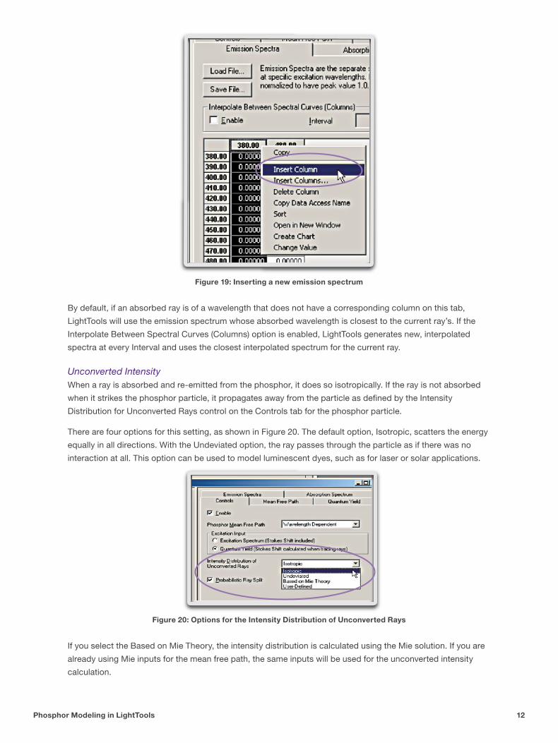
The data for both of these types exists in LightTools in tabular format, with one row per wavelength that

contains the wavelength value and the conversion percentage at that wavelength. A user can enter each of

the rows manually, or load a text file that allows all of the data to be entered at once. The format for the input

excitation spectrum data file is shown on page xx. The format for the input quantum yield data file is shown on

page 15. Figure 16 shows the Excitation Spectrum tab. Figure 17 shows the Quantum Yield tab.

Figure 16: The Excitation Spectrum tab

Equation 12


Figure 17: The Quantum Yield tab

Both the Excitation Spectrum and the Quantum Yield tabs have a field labeled Scale Factor. In both of these

cases, the Scale Factor directly modifies the absolute values of the data in the table without modifying the

relative shape. The scale factor is useful if you are using data that has been normalized and you need to

convert it to absolute values. In this case, enter the normalized values into the LightTools table, then set the

scale factor equal to the desired peak value.

Emission SpectraThe emission spectra, which define the spectrum of light emitted for any absorbed wavelength, must also be

specified. The tab that contains the emission spectra data is shown in Figure 18. This data can be entered

manually or via a text file, the format for which is shown on page 16.

Figure 18: The Emission Spectra tab

The data on the Emission Spectra tab is organized into columns that represent the emission spectrum vs.

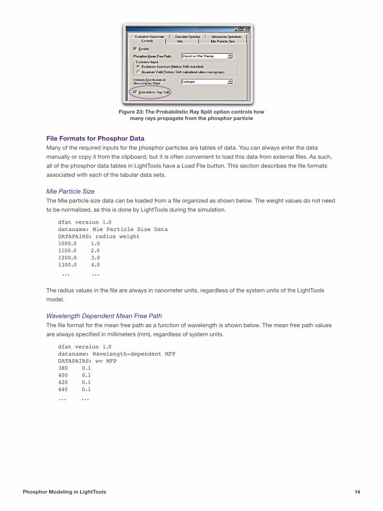
emission wavelength at a particular absorbed wavelength. You can insert a new emission spectrum by

selecting a column header, right-clicking, and choosing Insert Column, as shown in Figure 19.


Figure 19: Inserting a new emission spectrum

By default, if an absorbed ray is of a wavelength that does not have a corresponding column on this tab,

LightTools will use the emission spectrum whose absorbed wavelength is closest to the current ray’s. If the

Interpolate Between Spectral Curves (Columns) option is enabled, LightTools generates new, interpolated

spectra at every Interval and uses the closest interpolated spectrum for the current ray.

Unconverted IntensityWhen a ray is absorbed and re-emitted from the phosphor, it does so isotropically. If the ray is not absorbed

when it strikes the phosphor particle, it propagates away from the particle as defined by the Intensity

Distribution for Unconverted Rays control on the Controls tab for the phosphor particle.

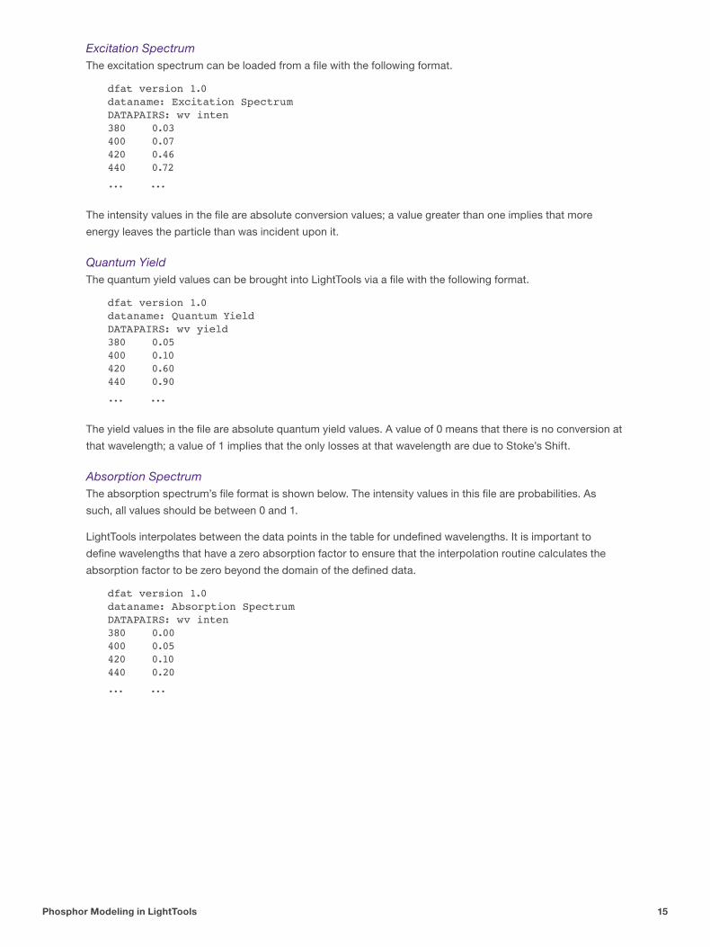
There are four options for this setting, as shown in Figure 20. The default option, Isotropic, scatters the energy

equally in all directions. With the Undeviated option, the ray passes through the particle as if there was no

interaction at all. This option can be used to model luminescent dyes, such as for laser or solar applications.

Figure 20: Options for the Intensity Distribution of Unconverted Rays

If you select the Based on Mie Theory, the intensity distribution is calculated using the Mie solution. If you are

already using Mie inputs for the mean free path, the same inputs will be used for the unconverted intensity

calculation.


The last type, User Defined, allows you to manually specify the intensity distribution. This option could be

used to enter a measured distribution. The intensity as a function of wavelength and angle is entered on the

Unconverted Intensity tab, shown in Figure 21.

Figure 21: Specifying a user-defined intensity distribution

The table consists of one column per wavelength and one row per angle. The angle is specified with respect to

the undeviated direction, as shown in Figure 22.

Figure 22: Graphical depiction of the unconverted intensity scatter angle

The Interpolate Between Separate Curves (Columns) option works the same way as the similar control on the

Emission Spectra tab. See “Emission Spectra” on page 11 for more information. The data in this table can also

be loaded from an external file. The format for the file is shown on page 16.

Number of Rays Propagating from the ParticleThe last control that must be considered for the phosphor particle is labeled Probabilistic Ray Split on the

Controls tab of the particle definition, as shown in Figure 23. By default, LightTools propagates one ray away

from the particle. If there is no conversion, this ray is the unconverted ray. If there is conversion, LightTools

probabilistically chooses whether to propagate the converted or unconverted ray. If this option is unchecked,

when conversion occurs, two rays propagate from the particle: the converted and the unconverted ray. Using

this option speeds up the ray trace, as fewer rays propagate through the system.

Insident ray

Scattered ray

Phosphorparticle

Angle ofscatter


Figure 23: The Probabilistic Ray Split option controls how many rays propagate from the phosphor particle

File Formats for Phosphor DataMany of the required inputs for the phosphor particles are tables of data. You can always enter the data

manually or copy it from the clipboard, but it is often convenient to load this data from external files. As such,

all of the phosphor data tables in LightTools have a Load File button. This section describes the file formats

associated with each of the tabular data sets.

Mie Particle SizeThe Mie particle size data can be loaded from a file organized as shown below. The weight values do not need

to be normalized, as this is done by LightTools during the simulation.

dfat version 1.0dataname: Mie Particle Size DataDATAPAIRS: radius weight1000.0 1.01100.0 2.01200.0 3.01300.0 4.0

... ...

The radius values in the file are always in nanometer units, regardless of the system units of the LightTools

model.

Wavelength Dependent Mean Free PathThe file format for the mean free path as a function of wavelength is shown below. The mean free path values

are always specified in millimeters (mm), regardless of system units.

dfat version 1.0dataname: Wavelength-dependent MFPDATAPAIRS: wv MFP380 0.1400 0.1420 0.1440 0.1

... ...


Excitation SpectrumThe excitation spectrum can be loaded from a file with the following format.

dfat version 1.0dataname: Excitation SpectrumDATAPAIRS: wv inten380 0.03400 0.07420 0.46440 0.72

... ...

The intensity values in the file are absolute conversion values; a value greater than one implies that more

energy leaves the particle than was incident upon it.

Quantum YieldThe quantum yield values can be brought into LightTools via a file with the following format.

dfat version 1.0dataname: Quantum YieldDATAPAIRS: wv yield380 0.05400 0.10420 0.60440 0.90

... ...

The yield values in the file are absolute quantum yield values. A value of 0 means that there is no conversion at

that wavelength; a value of 1 implies that the only losses at that wavelength are due to Stoke’s Shift.

Absorption SpectrumThe absorption spectrum’s file format is shown below. The intensity values in this file are probabilities. As

such, all values should be between 0 and 1.

LightTools interpolates between the data points in the table for undefined wavelengths. It is important to

define wavelengths that have a zero absorption factor to ensure that the interpolation routine calculates the

absorption factor to be zero beyond the domain of the defined data.

dfat version 1.0 dataname: Absorption SpectrumDATAPAIRS: wv inten 380 0.00400 0.05420 0.10440 0.20

... ...


Emission SpectraThe emission spectra can be loaded all at once from a file of the format shown below.

dfat version 1.0dataname: Emission SpectraDATAPAIRS: wv intenDATASETS: 2 380 480480 0.000 0.000490 0.275 0.275500 0.498 0.498510 0.705 0.705

... ... ...

Each column of the tab-delimited data set is the emission spectrum associated with a particular absorbed

wavelength. The DATASETS parameter identifies the number of absorbed wavelengths and, consequently,

how many columns of data, the file contains. The row immediately below the DATASETS parameter identifies

the absorbed wavelengths. The left-most value in this list corresponds to the left-most emission spectrum.

In order to ensure proper interpolation between the columns and the data points within a column, it is

important to make sure that the data in each column start and end with zero values.

User Defined Unconverted Intensity DistributionUser defined unconverted intensity files must be of the form shown below.

dfat version 1.0dataname: Unconverted IntensityDATAPAIRS: angle intenDATASETS: 1 5500 15 110 115 1

... ...

As with the emission spectra, this file can contain multiple columns of data: one for each of the defined

wavelengths. The DATASETS parameter identifies how many columns of data are present in the file. The line

immediately following the DATASETS line lists the wavelengths associated with each of the columns.

Measuring a Phosphor for Use in LightToolsAs you can see from the preceding sections, many inputs are required to build a proper phosphor model. In

summary, the necessary inputs are:

1. The absorption spectrum

2. The excitation spectrum/quantum yield

3. The mean free path

4. The emission spectra

5. The refractive index of the phosphor

Luckily, the first three inputs can be calculated from a simple inline transmission measurement. This section

discusses how to obtain the necessary phosphor inputs. See “Creating an LED Phosphor Model from

Measured Data” on page 20 to learn how these parameters are applied to various phosphor applications.


Obtaining Inline TransmissionThe inline transmission (Ti (λ)) is a convenient measurement that can be used to derive many of the required

inputs for a phosphor model. From this wavelength dependent set of values, the absorption spectrum, the

mean free path, and the excitation spectrum/quantum yield can be computed. There are several ways to

obtain the data.

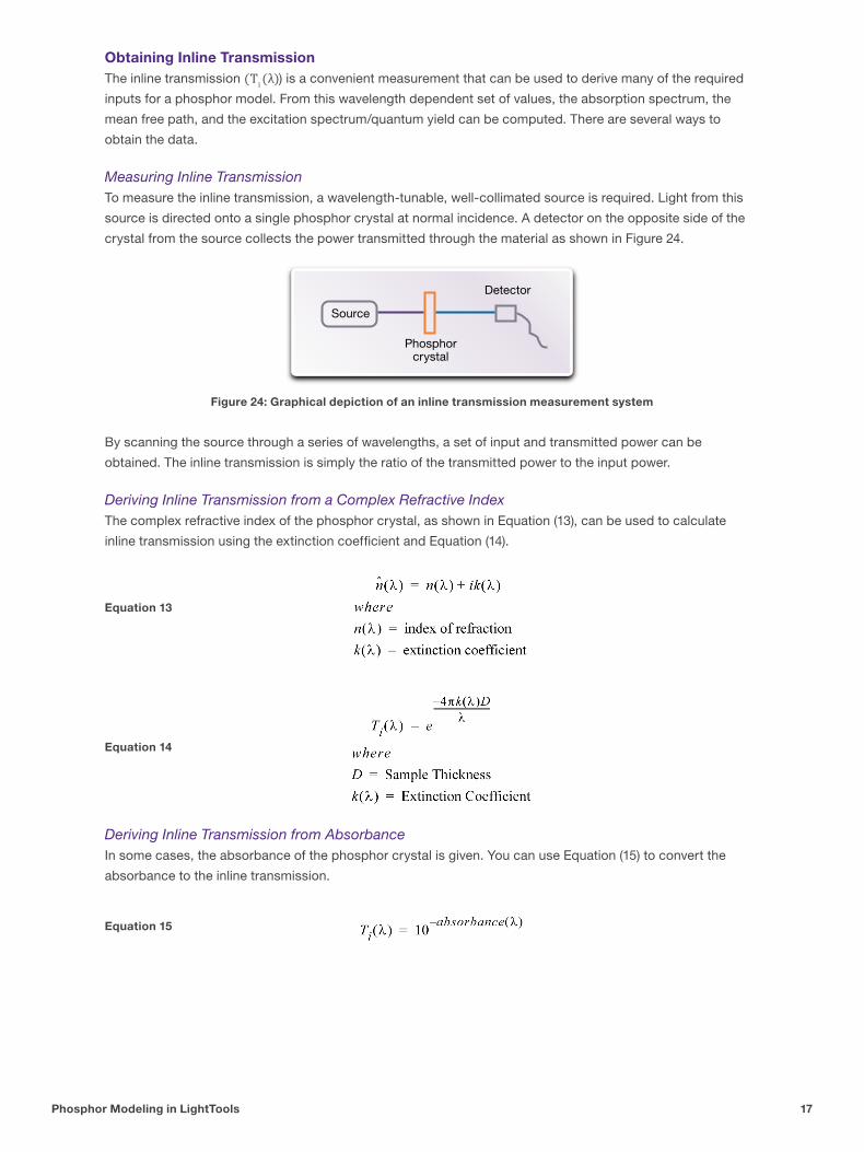
Measuring Inline TransmissionTo measure the inline transmission, a wavelength-tunable, well-collimated source is required. Light from this

source is directed onto a single phosphor crystal at normal incidence. A detector on the opposite side of the

crystal from the source collects the power transmitted through the material as shown in Figure 24.

Figure 24: Graphical depiction of an inline transmission measurement system

By scanning the source through a series of wavelengths, a set of input and transmitted power can be

obtained. The inline transmission is simply the ratio of the transmitted power to the input power.

Deriving Inline Transmission from a Complex Refractive IndexThe complex refractive index of the phosphor crystal, as shown in Equation (13), can be used to calculate

inline transmission using the extinction coefficient and Equation (14).

Deriving Inline Transmission from AbsorbanceIn some cases, the absorbance of the phosphor crystal is given. You can use Equation (15) to convert the

absorbance to the inline transmission.

Equation 13

Equation 14

Equation 15

Source

Detector

Phosphorcrystal


Calculating the Bulk Transmission of the Phosphor CrystalTo calculate a phosphor materials’ properties, the internal or bulk transmission of the crystal is needed. The

inline transmission contains the bulk transmission (Tb) as well as the losses due to Fresnel reflectance at

each of the faces of the crystal. Equation (16) shows the relationship between the bulk transmission, the inline

transmission, and the total Fresnel transmission (Tf).

The total Fresnel transmission is related to the total Fresnel reflectance (RF) by

The total Fresnel reflectance is the reflectance due to the first and second surface intersections as well as the

infinite other back reflections. The total Fresnel reflectance relates to the Fresnel reflectance of one surface

(R1F) by Equation (18).

For normal incidence, the Fresnel reflectance due to a single surface interaction is given by Equation (19) using

only the wavelength-dependent refractive index.

The contribution to the total Fresnel transmission of the high order reflections is small. Consequently, a good

approximation for Equation (17) is given in Equation (20).

Calculating the Absorption Spectrum and the Mean Free PathArmed with the bulk transmission from the previous section, you can now calculate the absorption spectrum

and the mean free path of the phosphor crystal. Equation (21) shows the relationship between all of these

values. In Equation (21), the absorption is shown to be wavelength dependent. You can also choose to have a

single absorption value and let the mean free path vary with wavelength.

It follows then that the absorption spectrum definition is given by Equation (22).

Since the absorption spectrum is a probability distribution, and we want the best probability that the phosphor

Equation 16

Equation 17

Equation 18

Equation 19

Equation 20

Equation 21

Equation 22


will work as expected, the absorption spectrum must be normalized. From Equation (22), it can be shown that

the maximum of the absorption spectrum occurs at the minimum value of the bulk transmission. Using this

concept gives

Setting the maximum absorption spectrum value equal to 1 allows us to solve for the mean free path, as

shown in Equation (24).

Obtaining the Quantum YieldThe best quantum yield value to use when modeling phosphors is one given by the manufacturer. The

quantum yield need only be a single value because as we’ve defined it, the absorption spectrum contains all

of the spectral information. Often, a quantum yield of 0.92 is reasonable if no other value can be obtained or

determined.

Calculating the Quantum Yield from the Inline TransmissionIf the quantum yield value is not given, you can derive it from the inline transmission. To understand how to

calculate the quantum yield value, consider the inline transmission measurement system’s energy balance.

The incident power (Φ0) is comprised of the absorbed power (Φα), the power lost to Fresnel reflections (ΦF), and the unabsorbed power (Φunα) as shown in Equation (25).

The re-emitted power (ΦEm), given by the absorbed power scaled by the quantum yield value and the Stoke’s

Shift, is the integrated spectral power distribution as shown in Equation (26).

The total emitted power cannot be obtained directly from the inline transmission measurement. Instead,

an integrating sphere and a spectrometer must be used to capture and measure the isotropically-emitted

radiation.

To calculate the Stoke’s Shift, a weighted average of the emitted wavelengths should be used. Equation

(27) shows the nominal relationship for the Stroke’s Shift and the weighting used to calculate the emitted

wavelength from the emission spectrum.

Equation 23

Equation 24

Equation 25

Equation 26

Equation 27


If you are using un-normalized values for the emission spectrum, Equation (27) becomes:

Combining Equation (25) and Equation (26) while dividing by Φ0 gives

You might notice that the last addend in Equation (29) is the inline transmission (Ti). The second to last term is

the total Fresnel reflectivity (RF). Substituting these values into Equation (29) gives Equation (30), the equation

for the quantum yield value.

It is important to note that in order to properly derive the quantum yield, the absorbed wavelength (λ0) and the

emission spectrum for that wavelength should not overlap. The calculation of the converted power (ΦEm) would

be skewed.

Obtaining the Emission SpectraOf all of the parameters that define a phosphor material, the emission spectra is the most likely to be given on

a data sheet. You can also measure the emission spectrum with an integrating sphere and a spectrometer.

Creating an LED Phosphor Model from Measured DataThere are two primary ways in which to use a phosphor inside of an LED: using a single, cut phosphor crystal

or using a particular density of small phosphor particles suspended in an encapsulant. When using a single

crystal, the measured data obtained in the previous section can be used directly as inputs, but when the

phosphor particles are in suspension, extra steps must be taken to ensure that a good model is achieved.

This section describes the process for creating each of these two phosphor models.

For a Single Phosphor CrystalThe inline transmission of the previous section is of a single crystal, and as such, the data derived from it can

be used directly as LightTools inputs. To create this kind of phosphor material, first follow Steps 1 and 2 as

described in “Creating a Phosphor Material in the LightTools User Interface” on page 5 to add a new material

with phosphor particles to the LightTools model.

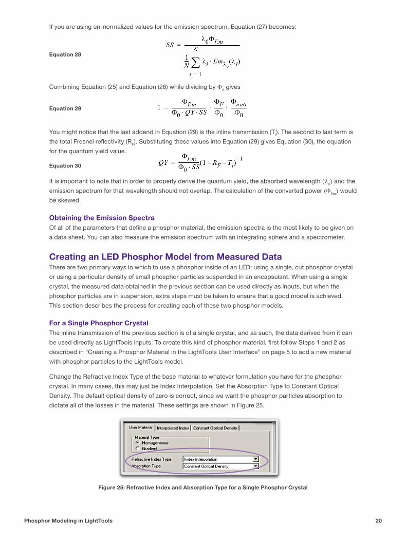
Change the Refractive Index Type of the base material to whatever formulation you have for the phosphor

crystal. In many cases, this may just be Index Interpolation. Set the Absorption Type to Constant Optical

Density. The default optical density of zero is correct, since we want the phosphor particles absorption to

dictate all of the losses in the material. These settings are shown in Figure 25.

Figure 25: Refractive Index and Absorption Type for a Single Phosphor Crystal

Equation 28

Equation 29

Equation 30


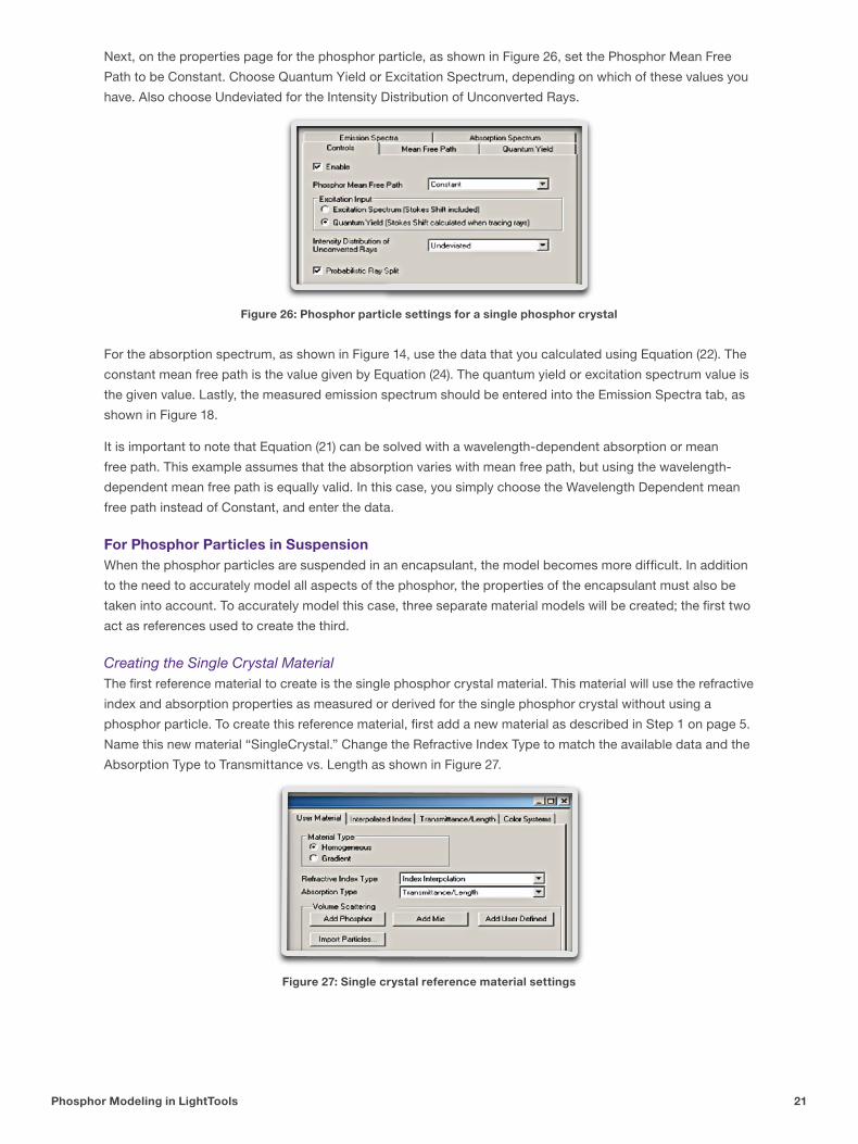
Next, on the properties page for the phosphor particle, as shown in Figure 26, set the Phosphor Mean Free

Path to be Constant. Choose Quantum Yield or Excitation Spectrum, depending on which of these values you

have. Also choose Undeviated for the Intensity Distribution of Unconverted Rays.

Figure 26: Phosphor particle settings for a single phosphor crystal

For the absorption spectrum, as shown in Figure 14, use the data that you calculated using Equation (22). The

constant mean free path is the value given by Equation (24). The quantum yield or excitation spectrum value is

the given value. Lastly, the measured emission spectrum should be entered into the Emission Spectra tab, as

shown in Figure 18.

It is important to note that Equation (21) can be solved with a wavelength-dependent absorption or mean

free path. This example assumes that the absorption varies with mean free path, but using the wavelength-

dependent mean free path is equally valid. In this case, you simply choose the Wavelength Dependent mean

free path instead of Constant, and enter the data.

For Phosphor Particles in SuspensionWhen the phosphor particles are suspended in an encapsulant, the model becomes more difficult. In addition

to the need to accurately model all aspects of the phosphor, the properties of the encapsulant must also be

taken into account. To accurately model this case, three separate material models will be created; the first two

act as references used to create the third.

Creating the Single Crystal MaterialThe first reference material to create is the single phosphor crystal material. This material will use the refractive

index and absorption properties as measured or derived for the single phosphor crystal without using a

phosphor particle. To create this reference material, first add a new material as described in Step 1 on page 5.

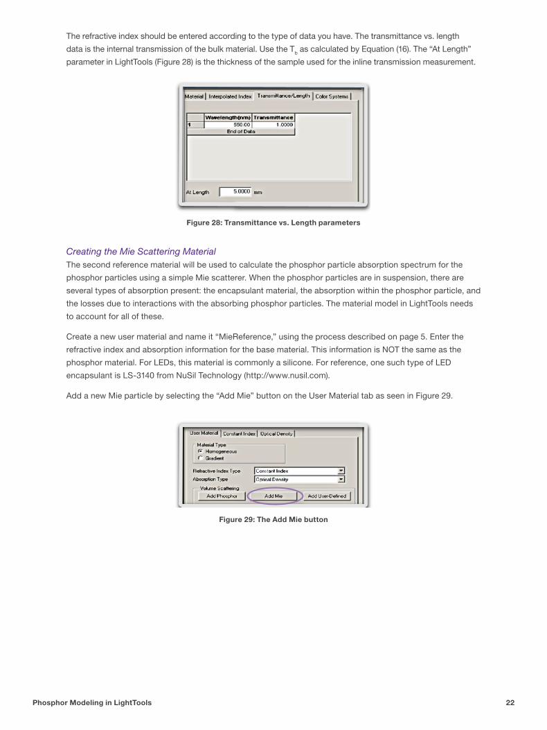
Name this new material “SingleCrystal.” Change the Refractive Index Type to match the available data and the

Absorption Type to Transmittance vs. Length as shown in Figure 27.

Figure 27: Single crystal reference material settings


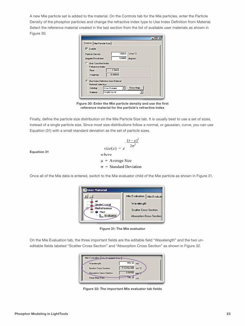
The refractive index should be entered according to the type of data you have. The transmittance vs. length

data is the internal transmission of the bulk material. Use the Tb as calculated by Equation (16). The “At Length”

parameter in LightTools (Figure 28) is the thickness of the sample used for the inline transmission measurement.

Figure 28: Transmittance vs. Length parameters

Creating the Mie Scattering MaterialThe second reference material will be used to calculate the phosphor particle absorption spectrum for the

phosphor particles using a simple Mie scatterer. When the phosphor particles are in suspension, there are

several types of absorption present: the encapsulant material, the absorption within the phosphor particle, and

the losses due to interactions with the absorbing phosphor particles. The material model in LightTools needs

to account for all of these.

Create a new user material and name it “MieReference,” using the process described on page 5. Enter the

refractive index and absorption information for the base material. This information is NOT the same as the

phosphor material. For LEDs, this material is commonly a silicone. For reference, one such type of LED

encapsulant is LS-3140 from NuSil Technology (http://www.nusil.com).

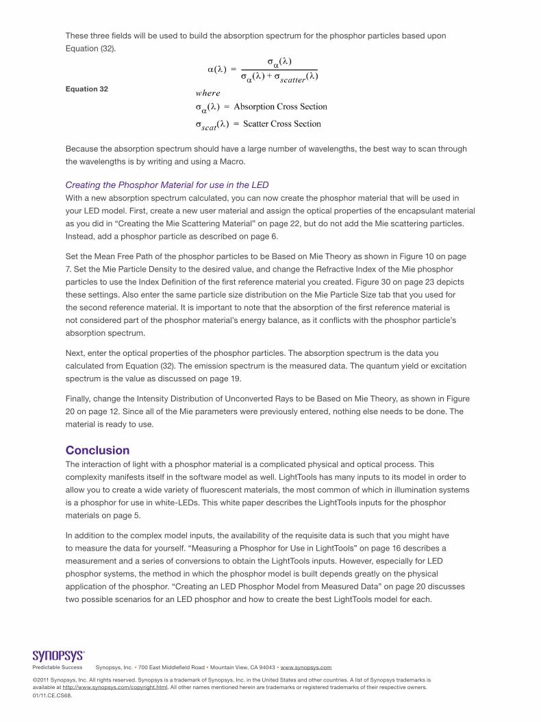
Add a new Mie particle by selecting the “Add Mie” button on the User Material tab as seen in Figure 29.

Figure 29: The Add Mie button


A new Mie particle set is added to the material. On the Controls tab for the Mie particles, enter the Particle

Density of the phosphor particles and change the refractive index type to Use Index Definition from Material.

Select the reference material created in the last section from the list of available user materials as shown in

Figure 30.

Figure 30: Enter the Mie particle density and use the first reference material for the particle’s refractive index

Finally, define the particle size distribution on the Mie Particle Size tab. It is usually best to use a set of sizes,

instead of a single particle size. Since most size distributions follow a normal, or gaussian, curve, you can use

Equation (31) with a small standard deviation as the set of particle sizes.

Once all of the Mie data is entered, switch to the Mie evaluator child of the Mie particle as shown in Figure 31.

Figure 31: The Mie evaluator

On the Mie Evaluation tab, the three important fields are the editable field “Wavelength” and the two un-

editable fields labeled “Scatter Cross Section” and “Absorption Cross Section” as shown in Figure 32.

Figure 32: The important Mie evaluator tab fields

Equation 31

Synopsys, Inc. 700 East Middlefield Road Mountain View, CA 94043 www.synopsys.com

©2011 Synopsys, Inc. All rights reserved. Synopsys is a trademark of Synopsys, Inc. in the United States and other countries. A list of Synopsys trademarks is available at http://www.synopsys.com/copyright.html. All other names mentioned herein are trademarks or registered trademarks of their respective owners.

01/11.CE.CS68.

These three fields will be used to build the absorption spectrum for the phosphor particles based upon

Equation (32).

Because the absorption spectrum should have a large number of wavelengths, the best way to scan through

the wavelengths is by writing and using a Macro.

Creating the Phosphor Material for use in the LEDWith a new absorption spectrum calculated, you can now create the phosphor material that will be used in

your LED model. First, create a new user material and assign the optical properties of the encapsulant material

as you did in “Creating the Mie Scattering Material” on page 22, but do not add the Mie scattering particles.

Instead, add a phosphor particle as described on page 6.

Set the Mean Free Path of the phosphor particles to be Based on Mie Theory as shown in Figure 10 on page

7. Set the Mie Particle Density to the desired value, and change the Refractive Index of the Mie phosphor

particles to use the Index Definition of the first reference material you created. Figure 30 on page 23 depicts

these settings. Also enter the same particle size distribution on the Mie Particle Size tab that you used for

the second reference material. It is important to note that the absorption of the first reference material is

not considered part of the phosphor material’s energy balance, as it conflicts with the phosphor particle’s

absorption spectrum.

Next, enter the optical properties of the phosphor particles. The absorption spectrum is the data you

calculated from Equation (32). The emission spectrum is the measured data. The quantum yield or excitation

spectrum is the value as discussed on page 19.

Finally, change the Intensity Distribution of Unconverted Rays to be Based on Mie Theory, as shown in Figure

20 on page 12. Since all of the Mie parameters were previously entered, nothing else needs to be done. The

material is ready to use.

ConclusionThe interaction of light with a phosphor material is a complicated physical and optical process. This

complexity manifests itself in the software model as well. LightTools has many inputs to its model in order to

allow you to create a wide variety of fluorescent materials, the most common of which in illumination systems

is a phosphor for use in white-LEDs. This white paper describes the LightTools inputs for the phosphor

materials on page 5.

In addition to the complex model inputs, the availability of the requisite data is such that you might have

to measure the data for yourself. “Measuring a Phosphor for Use in LightTools” on page 16 describes a

measurement and a series of conversions to obtain the LightTools inputs. However, especially for LED

phosphor systems, the method in which the phosphor model is built depends greatly on the physical

application of the phosphor. “Creating an LED Phosphor Model from Measured Data” on page 20 discusses

two possible scenarios for an LED phosphor and how to create the best LightTools model for each.

Equation 32

http://www.synopsys.com/copyright.html

phosphor modeling in lighttools - synopsys€¦ · · 2018-04-14phosphor modeling in lighttools...

Documents